A Hybrid Approach to Joint Estimation of Channel and Antenna impedance

Abstract

This paper considers a hybrid approach to joint estimation of channel information and antenna impedance, for single-input, single-output channels. Based on observation of training sequences via synchronously switched load at the receiver, we derive joint maximum a posteriori and maximum-likelihood (MAP/ML) estimators for channel and impedance over multiple packets. We investigate important properties of these estimators, e.g., bias and efficiency. We also explore the performance of these estimators through numerical examples.

I Introduction

Antenna impedance matching at mobile receivers has been shown to significantly impact capacity and diversity of wireless channels [1, 2, 5, 6, 3, 4]. This matching becomes challenging as antenna impedance changes with time-varying near-field loading, e.g., human users [9, 7, 8]. To mitigate this variation, joint channel and antenna impedance estimators have been derived under classical estimation assumptions [10, 11]. However, important properties of these estimators, e.g., bias and efficiency, remain unclear.

In this paper, we develop a hybrid estimation framework of channel information and antenna impedance, for single-input, single-output channels. In particular, channel information is modeled as complex Gaussian while antenna impedance is deterministic. Based on observation of training sequences via synchronously switched load at the receiver, we derive the joint maximum a posteriori and maximum-likelihood (MAP/ML) estimators for channel and impedance over multiple packets. Then, bias, consistency, and efficiency of these estimators are investigated. We also explore the performance of these estimators through numerical examples.

The rest of the paper is organized as follows. We present the system model in Sec. II, and derive the joint MAP/ML estimators for the channel and antenna impedance in Sec. III. Important properties, e.g., bias and efficiency, are studied in Sec. IV. We then explore the performance of these estimators through numerical examples in Sec. V, and conclude in Sec. VI.

II System Model

Consider a narrowband communications link with one transmit antenna and one receive antenna. We adopt the receiver model illustrated in Fig. 1, which has been widely used to model scenarios, where amplifier noise dominates at the receiver [4, 5, 6].

Fig. 1: Circuit model of a single-antenna receiver

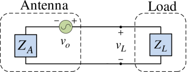
In Fig. 1, the antenna is modeled by its Thevenin equivalent

$$v\ =\ Z_{A}i+v_{o}\ ,$$ (1)

where $v,i\in\mathbb{C}$ are the voltage across, and current into, the antenna terminals. The antenna impedance is

$$Z_{A}\ =\ R_{A}+jX_{A}\ ,$$ (2)

where $R_{A}$ and $X_{A}$ are the resistance and reactance, respectively. In (1), $v_{o}\in\mathbb{C}$ is the open-circuit voltage induced by the incident signal field, which can be modeled in a flat-fading environment as [2]

$$v_{o}\ =\ Gx\ ,$$ (3)

where $x\in\mathbb{C}$ is the transmitted symbol and $G\in\mathbb{C}$ is the fading path gain. Suppose the fading path gain $G$ and antenna impedance $Z_{A}$ are unknown to the receiver. We assume the transmitter sends a predetermined training sequence, $x_{1},\ldots,x_{T}$, and the receiver shifts synchronously through a sequence of known impedances $Z_{L,1},\ldots,Z_{L,T}$. If $G$ and $Z_{A}$ are modeled as fixed over the duration of the training sequence, the observations are given by

$${v}_{L,t} = \frac{Z_{L,t}Gx_{t}}{Z_{A}+Z_{L,t}}+n_{t}\ ,~{}~{}~{}\ t=1,\ldots,T\ ,$$ (4)

where ${n}_{t}\sim\mathcal{CN}({0},\sigma_{n}^{2})$ are independent and identically distributed (i.i.d.) complex Gaussian noise. In this paper, we consider load impedances that take on only two possible values [10],

$$Z_{L,t}\ =\ \left\{\begin{array}[]{cc}Z_{1},&1\leq t\leq K\ ,\\ Z_{2},&K<t\leq T\ .\end{array}\right.$$ (7)

where $Z_{1}$ and $Z_{2}$ are known. Here we assume $Z_{L}=Z_{1}$ is the load impedance used to receive the transmitted data, and is matched to our best estimate of $Z_{A}$; additionally $Z_{L}=Z_{2}$ is an impedance variation introduced in order to make $Z_{A}$ observable.

The effective channel information needed by the communication algorithms is normally defined as [10, eq. 13],

$$H\ \triangleq\ \frac{Z_{1}G}{Z_{A}+Z_{1}}\ .$$ (8)

With this definition and (7), the sequence of observations in (4) can be described compactly in vector form,

$$\mathbf{v}_{L}\ \triangleq\ \begin{bmatrix}\mathbf{v}_{1}\\ \mathbf{v}_{2}\end{bmatrix}\ =\ \begin{bmatrix}H\mathbf{x}_{1}\\ FH\mathbf{x}_{2}\end{bmatrix}+\mathbf{n}\ ,$$ (9)

where the noise is i.i.d. complex Gaussian, $\mathbf{n}\sim\mathcal{CN}({0},\sigma_{n}^{2}\mathbf{I}_{T})$, the two partitions of each training sequence are,

$$\mathbf{x}_{1}\ \triangleq\ [x_{1},\dots,x_{K}]^{T}\ ,~{}~{}\mathbf{x}_{2}\ \triangleq\ [x_{K+1},\dots,x_{T}]^{T}\ ,$$ (10)

and $F$ is a one-to-one mapping of $Z_{A}$ provided $Z_{1}\neq Z_{2}$,

$$F\ \triangleq\ \frac{1+Z_{A}/Z_{1}}{1+Z_{A}/Z_{2}}\ .$$ (11)

Thus, knowing $F$ is equivalent to knowing $Z_{A}$.

Redefining the estimation problem in terms of $H$ and $F$ renders the observation bilinear in the unknowns. In the channel estimation literature, since $G$ usually results from a random superposition of multipaths, $H$ is usually modeled as a Gaussian random variable. On the other hand, $F$ appears more appropriately modeled as deterministic. This models the actual estimation problem better than the classical estimation model used in previous studies [10, 11]. In particular, the multi-packet estimators in the prequel assumed constant channel over all packets [10, Sec. V-B]. We consider in the next section the general and more important estimation problem, where the channel is time-varying over multiple packets and follows a complex Gaussian prior distribution.

III Joint MAP/ML Estimators

Consider a sequence of $L$ packets, where $H_{i}$ denotes the channel during the $i$-th packet transmission. We assume the channel information vector is unknown, jointly-distributed, complex Gaussian, such that

$$\mathbf{H}\ =\ [H_{1},\ldots,H_{L}]^{T}\sim{\cal CN}({\bf 0},\mathbf{C}_{\mathbf{H}})\ ,$$ (12)

where the channel covariance $\mathbf{C}_{\mathbf{H}}$ is known at the receiver. We assume $F$ changes more slowly with time, and is regarded as fixed over the $L$ packets. If each packet is formatted as (9), then the entire $L$ packets of observations can be written in matrix form,

$${\mathbf{V}}_{L}\ =\ \begin{bmatrix}\cdots&\mathbf{v}_{L,i}&\cdots\end{bmatrix}\ ,~{}~{}~{}1\leq i\leq L\ .$$ (13)

where each column is the observation of the $i$-th packet (9),

$$\mathbf{v}_{L,i}\ \triangleq\ \begin{bmatrix}\mathbf{v}_{1,i}\\ \mathbf{v}_{2,i}\end{bmatrix}\ =\ \begin{bmatrix}H_{i}\mathbf{x}_{1}\\ FH_{i}\mathbf{x}_{2}\end{bmatrix}+\mathbf{n}_{i}\ .$$ (14)

We assume the noise $\mathbf{n}_{i}\sim\mathcal{CN}({0},\sigma_{n}^{2}\mathbf{I}_{T})$ is temporally i.i.d.. The aim is to use these observations to estimate the unknowns

$${\boldsymbol{\theta}}\ \triangleq\ \begin{bmatrix}\mathbf{H}\\ F\end{bmatrix}\ .$$ (15)

Now we have precisely defined the estimation parameters and the observation model, it is important to identify an appropriate estimation framework. In classical estimation, unknown parameters are modeled as deterministic; in Bayesian estimation, they are modeled as random variables. The problem described in (15) is a hybrid estimation problem [13, pg. 329], because $\boldsymbol{\theta}$ contains both random and deterministic parameters. Several authors have investigated hybrid estimation problems [16, 15, 14, 17, 18]. Estimators and Cramér-Rao-type bounds for hybrid estimation were formulated in [14] in the context of passive source localization. In this section, we apply similar tools to address the estimation problem formulated in (15).

III-A Estimators for General ${\bf C}_{\mathbf{H}}$

Before discussing estimators, it is convenient to introduce sufficient statistics that summarize the information in the observations $\mathbf{V}_{L}$ in (13) relevant to estimation of $\boldsymbol{\theta}$. In classical estimation, a statistic ${\bf V}=f(\mathbf{V}_{L})$ is sufficient to estimate $\boldsymbol{\theta}$ based on $\mathbf{V}_{L}$ if $p(\mathbf{V}_{L}|{\mathbf{V}};\boldsymbol{\theta})=p({\mathbf{V}}_{L}|{\bf V})$. In Bayesian settings, a statistic is sufficient if $p({\mathbf{V}}_{L},{\boldsymbol{\theta}}|{\bf V})=p({\mathbf{V}}_{L}|{\bf V})p(\boldsymbol{\theta}|{\bf V})$. It is well known that classical sufficiency implies Bayesian sufficiency; it also clearly implies sufficiency for the hybrid estimation problem, which is defined in an analogous way.

A set of sufficient statistics to estimate $\boldsymbol{\theta}$ based on observations in (13) is derived in the Appendix. We therefore consider the observations to be the following vector in $\mathbb{C}^{2L}$,

$$\mathbf{V} \triangleq \begin{bmatrix}\mathbf{V}_{1}\\ \mathbf{V}_{2}\end{bmatrix}\ =\ \begin{bmatrix}\mathbf{H}+\mathbf{N}_{1}\\ F\mathbf{H}+\mathbf{N}_{2}\end{bmatrix}\ ,$$ (16)

where $\mathbf{N}_{1}\sim{\cal CN}({\bf 0},\frac{\sigma_{n}^{2}}{S_{1}}\mathbf{I}_{L})$ and $\mathbf{N}_{2}\sim{\cal CN}({\bf 0},\frac{\sigma_{n}^{2}}{S_{2}}\mathbf{I}_{L})$ are independent noise vectors, and we define

$$S_{1}\ \triangleq\ \mathbf{x}_{1}^{H}\mathbf{x}_{1}\ ,~{}~{}~{}S_{2}\ \triangleq\ \mathbf{x}_{2}^{H}\mathbf{x}_{2}\ .$$ (17)

Conditioned on $\mathbf{H}$, the sufficient statistic $\mathbf{V}$ is a complex Gaussian random vector, and its pdf is

$$p(\mathbf{V}|\mathbf{H};F)\ =\ \frac{\exp\left[-\left(\mathbf{V}-\boldsymbol{\mu}\right)^{H}\mathbf{C}_{\mathbf{v}}^{-1}\left(\mathbf{V}-\boldsymbol{\mu}\right)\right]}{\det(\pi\mathbf{C}_{\mathbf{v}})}\ ,$$ (18)

where the mean and covariance are, respectively,

$$\boldsymbol{\mu}\ =\ \begin{bmatrix}\mathbf{H}\\ F\mathbf{H}\end{bmatrix}\ ,~{}~{}\mathbf{C}_{\mathbf{v}}\ =\ \begin{bmatrix}\frac{\sigma_{n}^{2}}{S_{1}}\mathbf{I}_{L}&\mathbf{0}_{L\times L}\\ \mathbf{0}_{L\times L}&\frac{\sigma_{n}^{2}}{S_{2}}\mathbf{I}_{L}\end{bmatrix}\ .$$ (19)

Note $\mathbf{0}_{L\times L}$ represents the $L\times L$ all zero matrix. Also, we assume $F$ is an unknown constant and $\mathbf{H}$ is a random vector with pdf

$$p(\mathbf{H})\ =\ {[\det(\pi\mathbf{C}_{\mathbf{H}})]^{-1}}\exp\left(-\mathbf{H}^{H}\mathbf{C}_{\mathbf{H}}^{-1}\mathbf{H}\right)\ .$$ (20)

To jointly estimate $\mathbf{H}$ and $F$, we consider estimators that maximize the hybrid log-likelihood function [13, pg. 329][14],

$$\hat{\boldsymbol{\theta}}(\mathbf{V})\ \triangleq\ \arg\max_{\boldsymbol{\theta}\in\mathbb{C}^{L+1}}\,\ln\,p(\mathbf{V},\mathbf{H};F)\ ,$$ (21)

which are presented in the following theorem.

Theorem 1 (Joint MAP/ML Estimators)

Given the sufficient statistic $\mathbf{V}$ in (16), the joint MAP/ML estimators for $\mathbf{H}$ and $F$ are, respectively,

$$\hat{\bf H}_{MAP}\ \triangleq\ \mathbf{A}\left(\hat{F}_{ML}\right)\left(\mathbf{V}_{1}+\alpha\hat{F}_{ML}^{*}\mathbf{V}_{2}\right)\ ,$$ (22)

and $\hat{F}_{ML}$, where $\hat{F}_{ML}$ is a zero of the rational function

$$g(F) \triangleq \left(\mathbf{V}_{1}+\alpha F^{*}\mathbf{V}_{2}\right)^{H}\mathbf{A}^{H}(F)\mathbf{A}(F)$$ (23)

$$\cdot\left(\mathbf{V}_{2}-F\mathbf{V}_{1}+\frac{\sigma_{n}^{2}}{S_{1}}{\mathbf{C}}_{\mathbf{H}}^{-1}\mathbf{V}_{2}\right)\ ,$$

and we define

$$\alpha\ \triangleq\ \frac{S_{2}}{S_{1}}\ ,~{}~{}~{}\mathbf{A}(F)\ \triangleq\ \left[\left(1+\alpha|F|^{2}\right)\mathbf{I}+\frac{\sigma_{n}^{2}}{S_{1}}\mathbf{C}_{\mathbf{H}}^{-1}\right]^{-1}\ .$$ (24)

Proof:

From (18) and (20), we write the (hybrid) log-likelihood function as

$$\mathcal{L}(\boldsymbol{\theta})\ \triangleq\ \ln\,p(\mathbf{V},\mathbf{H};F)=\ln\,[p(\mathbf{V}|\mathbf{H};F)\,p(\mathbf{H})]$$

$$= -\frac{S_{1}}{\sigma_{n}^{2}}|\mathbf{V}_{1}-\mathbf{H}|^{2}-\frac{S_{2}}{\sigma_{n}^{2}}|\mathbf{V}_{2}-F\mathbf{H}|^{2}-\mathbf{H}^{H}\mathbf{C}_{\mathbf{H}}^{-1}\mathbf{H}+C\ ,$$

where $C$ is a constant, and $S_{1}$ and $S_{2}$ are defined in (17). If we denote the real and imaginary parts of the parameter vector by $\boldsymbol{\theta}=\boldsymbol{\theta}_{r}+j\boldsymbol{\theta}_{i}$, the (complex) gradient is given by [12, Sec. 15.6]

$$\frac{\partial\mathcal{L}(\boldsymbol{\theta})}{\partial\boldsymbol{\theta}^{*}}\ \triangleq\ \frac{1}{2}\left[\frac{\mathcal{L}(\boldsymbol{\theta})}{\partial\boldsymbol{\theta}_{r}}+j\frac{\mathcal{L}(\boldsymbol{\theta})}{\partial\boldsymbol{\theta}_{i}}\right]\ .$$ (26)

In order for $\boldsymbol{\theta}$ in (15) to maximize the log-likelihood $\mathcal{L}(\boldsymbol{\theta})$, it is necessary that the gradient $\frac{\partial\mathcal{L}(\boldsymbol{\theta})}{\partial\boldsymbol{\theta}^{*}}$ vanishes, i.e.,

$$\begin{bmatrix}\frac{S_{1}}{\sigma_{n}^{2}}(\mathbf{V}_{1}-\mathbf{H})+\frac{S_{2}}{\sigma_{n}^{2}}(\mathbf{V}_{2}-F\mathbf{H})F^{*}-{\bf C}_{\mathbf{H}}^{-1}\mathbf{H}\\ \frac{S_{2}}{\sigma_{n}^{2}}\mathbf{H}^{H}(\mathbf{V}_{2}-F\mathbf{H})\end{bmatrix}\ =\ {\bf 0}\ .$$ (27)

Solving the first equation for $\mathbf{H}$, we obtain (22). To find $F$, substitute (22) into the second equation, which yields (23). $\hfill\diamond$ ∎

Since $g(F)$ is a ratio of polynomials, it may have multiple zeros, so Theorem 1 does not necessarily specify unique estimators. Given multiple zeros $F_{1},...,F_{m}$, however, we can identify the MAP/ML solution: For each $F_{j}$, we can, in principle, calculate a corresponding estimate of $\mathbf{H}_{j}$ from (22). The MAP/ML solution will be the pair $\hat{\boldsymbol{\theta}_{j}}=[\mathbf{H}_{j}^{T},F_{j}]^{T}$ that maximizes $\mathcal{L}(\boldsymbol{\theta})$.

III-B Special Cases of $\sigma_{n}^{-2}\mathbf{C}_{\mathbf{H}}$

We now consider three extreme cases of $\sigma_{n}^{-2}\mathbf{C}_{\mathbf{H}}$ in which Theorem 1 yields explicit, closed-form estimators for $\mathbf{H}$ and $F$. First suppose $\mathbf{H}$ (12) is an i.i.d. sequence, so $\mathbf{C}_{\mathbf{H}}=\sigma_{H}^{2}\mathbf{I}$. Thus, $g(F)=0$ reduces to,

$$\left(\mathbf{V}_{1}+\alpha F^{*}\mathbf{V}_{2}\right)^{H}\left(\mathbf{V}_{2}-cF\mathbf{V}_{1}\right)\ =\ 0\ ,$$ (28)

where

$$c\ \triangleq\ {S_{1}\sigma_{H}^{2}}/({S_{1}\sigma_{H}^{2}+\sigma_{n}^{2}})\ .$$ (29)

Expanding the product and defining $P_{ij}\triangleq(1/L)\mathbf{V}_{i}^{H}\mathbf{V}_{j}$, we obtain

$$P_{12}+(\alpha P_{22}-cP_{11})F-\alpha cP_{21}F^{2}\ =\ 0\ .$$ (30)

The ML estimate of $F$ is given by one of two roots,

$$F=\frac{\alpha P_{22}-cP_{11}\pm\sqrt{(\alpha P_{22}-cP_{11})^{2}+4\alpha c|P_{21}|^{2}}}{2c\alpha P_{21}}\ .$$ (31)

We conjecture the positive root above is always the joint ML estimate; however, as noted earlier, we can determine which root is the MAP/ML solution by identifying the root that maximizes $\mathcal{L}(\boldsymbol{\theta})$.

The second extreme case we consider is an arbitrary non-singular ${\bf C}_{\mathbf{H}}$ in the low noise limit, $\sigma_{n}^{2}\rightarrow 0$. In (23), applying the approximation $\sigma_{n}^{2}{\bf C}_{\mathbf{H}}^{-1}\approx{\bf 0}$, $g(F)=0$ leads to

$$\left(\mathbf{V}_{1}+\alpha F^{*}\mathbf{V}_{2}\right)^{H}\left(\mathbf{V}_{2}-F\mathbf{V}_{1}\right)\ =\ 0\ .$$ (32)

Comparing this to (28), we see this equation is identical to the case of i.i.d. $\mathbf{H}$ for $c=1$. It follows immediately that the ML estimate of $F$ is given by one of the following two roots,

$$F=\frac{\alpha P_{22}-P_{11}\pm\sqrt{(\alpha P_{22}-P_{11})^{2}+4\alpha|P_{21}|^{2}}}{2\alpha P_{21}}\ .$$ (33)

This result suggests that the ML estimator for arbitrary non-singular ${\bf C}_{\mathbf{H}}$ is asymptotically the same as the i.i.d. ML estimator in (31) in the low-noise or high SNR limit.

Finally, the last extreme case we consider is the single-packet case, i.e., $L=1$, where $\mathbf{H}=H\sim\mathcal{CN}(0,\sigma_{H}^{2})$ is a special case of (20). Under these assumptions, the sufficient statistic in (16) becomes $\mathbf{V}=[V_{1},V_{2}]^{T}$, and Theorem 1 leads to the single-packet joint MAP/ML solution,

$$\hat{\boldsymbol{\theta}}_{SP}\ =\ \begin{bmatrix}\hat{H}_{MAP}&\hat{F}_{ML}\end{bmatrix}^{T}\ =\ \begin{bmatrix}cV_{1}&\frac{V_{2}}{cV_{1}}\end{bmatrix}^{T}\ ,$$ (34)

where $c$ is defined in (29). Note two sets of solutions exist for (27), i.e., $\hat{\boldsymbol{\theta}}_{SP}$ as in (34) and $\hat{\boldsymbol{\theta}_{2}}=[0,-V_{1}^{*}/(\alpha V_{2}^{*})]^{T}$. Substituting each back into the single-packet log-likelihood, it can be shown that

$$\mathcal{L}(\hat{\boldsymbol{\theta}}_{SP})=-\frac{S_{1}}{\sigma_{n}^{2}}|V_{1}|^{2}(1-c)\geq\mathcal{L}(\hat{\boldsymbol{\theta}_{2}})=-\frac{S_{1}}{\sigma_{n}^{2}}|V_{1}|^{2}-\frac{S_{2}}{\sigma_{n}^{2}}|V_{2}|^{2}\ ,$$

for all $V_{1},V_{2},0<c<1$. So (34) is the global maximum of $\mathcal{L}(\boldsymbol{\theta})$, and thus the single-packet joint MAP/ML estimators.

The extremely slow fading case is mathematically identical to the single-packet case, where $\mathbf{H}=H{\bf 1}$, and $\bf 1$ is the all one vector. Its joint MAP/ML solution follows directly from (34), by regarding all $L$ packets as one large packet of size $LT$.

IV Properties of the Joint MAP/ML Estimators

The performance of estimators is often measured by low-order central moments, such as bias and mean-squared error (MSE). In this section, we explore the behavior of these moments for the joint MAP/ML estimators in Theorem 1, as well as the consistency of these estimators.

IV-A Single-Packet Estimators

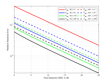
First consider the single-packet estimators in (34). Clearly $\hat{H}_{MAP}$ is complex Gaussian, and has finite MSE. But $\hat{F}_{ML}$ in (34) is a ratio of two joint complex Gaussian random variables with zero mean. The mean of general complex Gaussian ratios has been derived in closed-form[19, eq. 3]. Based on this result, we show the joint ML estimator in $\hat{F}_{ML}$ is unbiased, i.e., $E[\hat{F}_{ML}]=F$ for all $F\in\mathbb{C}$. However, its MSE, $E[|\hat{F}_{ML}-F|^{2}]$, is unbounded. Consequently, mean absolute error (MAE) is used instead of MSE in the simulations when the single-packet $\hat{F}_{ML}$ (34) is plotted (e.g., see Fig. 6).

IV-B Consistency

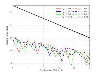
Except for the single-packet (or slow-fading) case (34), it appears difficult to evaluate the mean of $\hat{F}_{ML}$ for $L>1$, although numerical examples suggest it may be biased (see Fig. 4). To gain insight into its bias, we study the consistency of $\hat{F}_{ML}$ for i.i.d. $\mathbf{H}$ when $L$ becomes large. By definition, an estimator $\hat{F}$ is consistent if, given any $\epsilon>0$ [12, pg. 200], it converge in probability to the true parameter, $\lim\limits_{L\rightarrow\infty}\Pr(|\hat{F}-F|>\epsilon)=0$. As $L\rightarrow\infty$, the coefficients in (30) converge in probability,

$$\lim_{L\rightarrow\infty}P_{11} = \sigma_{H}^{2}+\sigma_{n}^{2}/S_{1}\ ,~{}~{}\lim_{L\rightarrow\infty}P_{21}\ =\ \sigma_{H}^{2}F^{*}\ ,$$

$$\lim_{L\rightarrow\infty}P_{22} = |F|^{2}\sigma_{H}^{2}+\sigma_{n}^{2}/S_{2}\ ,$$

so the roots (31) converge to

$$\left[\alpha|F|^{2}-cd\pm\sqrt{(\alpha|F|^{2}-cd)^{2}+4\alpha c|F|^{2}}\right]/{2\alpha cF^{*}}\ ,$$ (35)

where $d\triangleq 1-(\sigma_{n}^{2}/S_{1}\sigma_{H}^{2})^{2}$. Since neither root converges to $F$, it follows the joint ML estimator $\hat{F}_{ML}$ is inconsistent in $L$. However, if the second term in the square root in (35) is multiplied by $d$ (to complete the square), the positive root becomes $F/c$. This suggests a consistent estimator

$$\hat{F}_{C}\ \triangleq\ \frac{\alpha P_{22}-cP_{11}+\sqrt{(\alpha P_{22}-cP_{11})^{2}+4\alpha cd|P_{21}|^{2}}}{2\alpha P_{21}}\ .$$ (36)

For large signal-to-noise ratios ($S_{1}\sigma_{H}^{2}\gg\sigma_{n}^{2}$), we note $c$ and $d$ are approximately 1, and the positive root in (31) coincides with this consistent estimator. In the next section, we will compare the performance of $\hat{F}_{ML}$ and $\hat{F}_{C}$ via simulations.

IV-C Hybrid Cramér-Rao Bound

To evaluate estimator performance, it is useful to consider a fundamental lower bound on the error covariance

$${\bf C}_{\hat{\boldsymbol{\theta}}}\ \triangleq\ E_{\mathbf{V},\mathbf{H};F}\left[\left(\hat{\boldsymbol{\theta}}-{\boldsymbol{\theta}}\right)\left(\hat{\boldsymbol{\theta}}-{\boldsymbol{\theta}}\right)^{H}\right]\ ,$$ (37)

where $E_{\mathbf{V},\mathbf{H};F}$ denotes expectation with respect to the pdf $p(\mathbf{V},\mathbf{H};F)$, which is the product of (18) and (20). A Cramér-Rao Bound for the hybrid estimation problem was presented in [13, pg. 329],[14]. Let $\mathcal{L}(\boldsymbol{\theta})$ be the hybrid log-likelihood in (III-A), and define the pseudo-information as

$$E_{\mathbf{V},\mathbf{H};F}\left[\left(\frac{\partial\mathcal{L}(\boldsymbol{\theta})}{\partial\boldsymbol{\theta}^{*}}\right)\left(\frac{\partial\mathcal{L}(\boldsymbol{\theta})}{\partial\boldsymbol{\theta}^{*}}\right)^{T}\right]\ .$$ (38)

The hybrid CRB (HCRB) states that, if the pseudo-information vanishes, then

$${\bf C}_{\hat{\boldsymbol{\theta}}}\ \geq\ \boldsymbol{\mathcal{I}}^{-1}\ ,$$ (39)

for any $\hat{\boldsymbol{\theta}}=[\hat{\mathbf{H}}^{T},\hat{F}]^{T}$ such that $\hat{F}$ is unbiased, where $\boldsymbol{\mathcal{I}}$ is the hybrid information matrix,

$$\boldsymbol{\mathcal{I}}\ \triangleq\ E_{\mathbf{V},\mathbf{H};F}\left[\left(\frac{\partial\mathcal{L}(\boldsymbol{\theta})}{\partial\boldsymbol{\theta}^{*}}\right)\left(\frac{\partial\mathcal{L}(\boldsymbol{\theta})}{\partial\boldsymbol{\theta}^{*}}\right)^{H}\right]\ .$$ (40)

For the estimation problem (15), from (27) it is easy to verify that the pseudo-information (38) vanishes, and the HCRB is

$${\bf C}_{\hat{\boldsymbol{\theta}}}\ \geq\begin{bmatrix}\left[\left(\frac{S_{1}+|F|^{2}S_{2}}{\sigma_{n}^{2}}\right)\mathbf{I}+\mathbf{C}_{\mathbf{H}}^{-1}\right]^{-1}&{\bf 0}_{L\times 1}\\ {\bf 0}_{1\times L}&\frac{\sigma_{n}^{2}}{S_{2}{\rm Tr}[\mathbf{C}_{\mathbf{H}}]}\end{bmatrix}\ .$$ (41)

Note that uncertainty in $\mathbf{H}$ affects the estimators differently. For example, doubling all eigenvalues of $\mathbf{C}_{\mathbf{H}}$ makes $p(\mathbf{H})$ less informative, and increases the lower bound on $\hat{\mathbf{H}}$ error covariance, but decreases the error bound on $F$ estimation. This is intuitively reasonable, since a larger $\operatorname{Tr}[\mathbf{C}_{\mathbf{H}}]$ essentially increases the signal-to-noise of the observation of $F$.

V Numerical Results

Fig. 2: Relative MSE of $\hat{\mathbf{H}}_{MAP}$ versus SNR.

Fig. 3: MSE of $\hat{F}_{ML}$ and $\hat{F}_{C}$ against SNR for $L>2$.

In this section, we explore the performance of the estimators in Secs. III-IV through numerical examples. We take the training sequence in (9) as a unit-magnitude Zadoff-Chu sequence of length $T=64$. The unknown antenna impedance is that of a dipole $Z_{A}=73+j42.5\,\Omega$. The load impedance (7) is $Z_{1}=50\,\Omega$ for the first $K=T/2=32$ symbols of each training sequence, and $Z_{2}=50+j20\,\Omega$ for the remaining symbols. From (11), it follows $F=0.9860+j0.2445$. Suppose the channel $\mathbf{H}$ is an i.i.d. sequence, so ${\bf C}_{\mathbf{H}}=\sigma_{H}^{2}\mathbf{I}$, and define the post-detection signal-to-noise ratio (SNR) of a training symbol as

$$\rho\ \triangleq\ {\sigma_{H}^{2}}/{\sigma_{n}^{2}}\ .$$ (42)

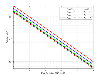
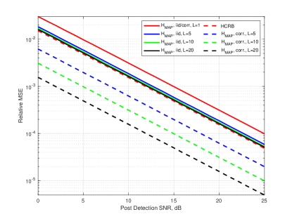
In Fig. 2, we plot the relative mean-squared error (MSE) of the MAP estimator (22), which is defined as $E[\parallel\hat{\mathbf{H}}_{MAP}-\mathbf{H}\parallel^{2}]/L\sigma_{H}^{2}$, versus $\rho$ for $L=1,2,5,10$ training packets. Here $\hat{F}_{ML}$ is the positive root of (31). Also shown is the HCRB bound on $\hat{\mathbf{H}}_{MAP}$, which equals the diagonal elements of the upper left matrix block in HCRB (41). This HCRB also lower bounds any channel estimator given $F$. Note the single-packet estimator (34) is 3 dB away from the HCRB, since it uses only half of the training symbols. When even a few packets are combined, however, the improved estimate of $F$ enables $\hat{\mathbf{H}}_{MAP}$ to quickly approach the HCRB to within a fraction of a dB. In particular, for $L=10$, the efficiency is above 90% for all SNR plotted.

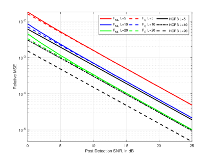
If we assume the MSE of $\hat{F}_{ML}$ is finite for $L>2$, we can compare its MSE performance to HCRB derived in (41), which, however, is often loose and unachievable[16]. In Fig. 3, we plot the relative MSE, $E[|\hat{F}_{ML}-F|^{2}]/|F|^{2}$ versus SNR for $L=5,10,20$. At low SNRs, we observe that $\hat{F}_{ML}$ diverges somewhat from the straight line it traces at high SNR. One possible explanation for this behavior is the presence of bias in $\hat{F}_{ML}$ at low SNRs. Some support for this hypothesis was given in Sec. IV-B, where we showed that $\hat{F}_{ML}$ is inconsistent in $L$. To remedy this situation, we defined a consistent estimator $\hat{F}_{C}$ in (36), which is also plotted in Fig. 3. We observe that $\hat{F}_{C}$ performs as well or better than $\hat{F}_{ML}$ for all SNR and $L$ in the figure. In particular, $\hat{F}_{C}$ outperforms $\hat{F}_{ML}$ at low SNR. Back in Fig. 2, we also plotted $\hat{\mathbf{H}}_{C}$, which substitutes $\hat{F}_{C}$ in (22) instead of $\hat{F}_{ML}$. However, both channel estimators appear to coincide for all SNR and $L$ plotted.

To better understand the impact of bias, in Fig. 4 we plot the absolute relative bias, defined as $|E[\hat{F}_{ML}-F]/{F}|$, versus SNR for $L=5,10$ and two values of $F$, i.e., $F_{1}=0.9860+j0.2445$ and $F_{2}=1.0644+j0.5451$. Note all four curves for $\hat{F}_{ML}$ seem to coincide, and suggest a relative bias that decreases with SNR but does not appear to depend on $L$ or $F$. For comparison, we also plot the corresponding curves for the consistent estimator, $\hat{F}_{C}$. Compared with $\hat{F}_{ML}$, the bias of $\hat{F}_{C}$ at low and medium SNR appears two orders of magnitude smaller, and does not suggest dependence on $L$. We do not know if $\hat{F}_{C}$ is unbiased, but it appears less biased than $\hat{F}_{ML}$.

Fig. 4: Relative Bias of $\hat{F}_{ML}$ versus SNR and $L$.

Thus far, we have assumed $\mathbf{H}$ is i.i.d. Now consider an example of extremely slow fading, where $H_{1}=\cdots=H_{L}$. In Fig. 5, we plot the relative MSE of $\hat{H}_{MAP}$ versus SNR for several values of $L$. The performance of $\hat{\mathbf{H}}_{MAP}$ (22) for i.i.d. $\mathbf{H}$ is also included for comparison. Not surprisingly, strong correlation in $\mathbf{H}$ leads to a smaller MSE for $L>1$, since each channel is now averaged over $L$ observations. However, it is worth noting the opposite is true of $\hat{F}_{ML}$. In Fig. 6, we plot the relative MAE of $\hat{F}_{ML}$, i.e., $E[|\hat{F}_{ML}-F|]/|F|$, under the same conditions as Fig. 5. Here the i.i.d. channel leads to considerably better estimates of $F$, since multiple, independent channel observations average out variations due to $\mathbf{H}$.

Fig. 5: Relative MSE of $\hat{H}_{MAP}$ versus SNR for a correlated channel.

Fig. 6: Relative MAE of $\hat{F}_{ML}$ versus SNR for a correlated channel.

VI Conclusions

In this paper, we developed a hybrid estimation framework for joint estimation of channel information and antenna impedance. Joint maximum a posteriori and maximum-likelihood (MAP/ML) estimators are derived for multi-packet scenarios in a temporally correlated fading channel. Important properties, e.g., efficiency and/or bias, are investigated for the joint MAP/ML estimators, either analytically or through numerical means. We found the joint ML estimators for $F$ are generally biased, except for the single-packet case. After studying its consistency, we found a consistent estimator, which performs as well or better than the joint ML estimator in terms of bias and MSE. Furthermore, the joint MAP channel estimator becomes efficient with a sufficient number of packets. We also explored the impact of channel correlation on estimation accuracy to find that correlation improves channel estimation but worsens impedance estimation.

Rearrange the conditional PDF $p\left(\mathbf{v}_{L,i};\boldsymbol{\theta}\right)$ of any arbitrary $\mathbf{v}_{L,i}$ defined in (14), $1\leq i\leq L$,

$$\exp\left(-\frac{S_{1}|V_{1,i}-H|^{2}}{\sigma_{n}^{2}}-\frac{S_{2}|V_{2,i}-FH|^{2}}{\sigma_{n}^{2}}\right)g(\mathbf{v}_{L,i})\ ,$$

where $g(\mathbf{v}_{L,i})$ only depends on $\mathbf{v}_{L,i}$ (and known training sequences $\mathbf{x}_{1}$ and $\mathbf{x}_{2}$), but not $\boldsymbol{\theta}$,

$$g(\mathbf{v}_{L,i})\ \triangleq\ {(\pi\sigma_{n}^{2})^{-T}}\exp\left[\frac{1}{\sigma_{n}^{2}}(V_{1,i}+V_{2,i}-{|\mathbf{v}_{L,i}|^{2}})\right]\ ,$$

and we define

$$V_{1,i}\ \triangleq\ {\mathbf{x}_{1}^{H}\mathbf{v}_{1,i}}/{S_{1}}\ ,~{}~{}~{}V_{2,i}\ \triangleq\ {\mathbf{x}_{2}^{H}\mathbf{v}_{2,i}}/{S_{2}}\ .$$ (43)

By Neyman-Fisher factorization Theorem [12, pg. 117], $V_{1,i}$ and $V_{2,i}$ is a set of sufficient statistic. To get (16), combine all $L$ sets of sufficient statistics in vector form, i.e., $\mathbf{V}_{1}=[\cdots~{}V_{1,i}~{}\cdots]^{T}$, and $\mathbf{V}_{2}=[\cdots~{}V_{2,i}~{}\cdots]^{T}$. $\hfill\diamond$

References

- [1] C. P. Domizioli and B. L. Hughes, “Noise correlation in compact diversity receivers,” IEEE Trans. Commun., vol. 58, no. 5, pp. 1426–1436, May 2010.
- [2] C. P. Domizioli and B. L. Hughes, “Front-end design for compact MIMO receivers: A communication theory perspective,” IEEE Trans. Commun., vol. 60, no. 10, pp. 2938–2949, Oct. 2012.
- [3] M. J. Gans, “Channel capacity between antenna Arrays - Part I: sky noise dominates,” IEEE Trans. Commun., vol. 54, no. 9, pp. 1586–1592, Sep. 2006.
- [4] M. J. Gans, “Channel capacity between antenna arrays - Part II: Amplifier noise dominates,” IEEE Trans. Commun., vol. 54, no. 11, pp. 1983–1992, Nov. 2006.
- [5] B. K. Lau, J. B. Andersen, G. Kristensson and A. F. Molisch, “Impact of Matching Network on Bandwidth of Compact Antenna Arrays,” IEEE Trans. Antennas Propag., vol. 54, no. 11, pp. 3225–3238, Nov. 2006.
- [6] J. W. Wallace and M. A. Jensen, “Mutual Coupling in MIMO Wireless Systems: A Rigorous Network Theory Analysis,” IEEE Trans. Wireless Commun., vol. 3, no. 4, pp 1317–1325, Jul. 2004
- [7] S. M. Ali, M. Buckley, J. Deforge, J. Warden and A. Danak, “Dynamic Measurement of Complex Impedance in Real-Time for Smart Handset Applications,” IEEE Trans. Microw. Theory Techn., vol. 61, no. 9, pp. 3453–3460, Aug. 2013.
- [8] R. Mohammadkhani and J. S. Thompson, “Adaptive Uncoupled Termination for Coupled Arrays in MIMO Systems,” IEEE Trans. Antennas Propag., vol. 61, no. 8, pp. 4284–4295, May 2013.
- [9] I. Vasilev, V. Plicanic and B. K. Lau, “Impact of Antenna Design on MIMO Performance for Compact Terminals With Adaptive Impedance Matching,” IEEE Trans. Antennas Propag., vol. 64, no. 4, pp. 1454–1465, Jan. 2016.
- [10] S. Wu and B. L. Hughes, “Training-based joint channel and impedance estimation,” IEEE 2018 52nd Annual Conference on Information Sciences and Systems (CISS), pp. 1–6, Princeton University, NJ, Mar. 2018.
- [11] Y. Hassan and A. Wittneben, “Joint spatial channel and coupling impedance matrices estimation in compact MIMO systems: The use of adaptive loads,” IEEE Intl. Symp. on Personal, Indoor and Mobile Radio Commun., PIMRC, pp. 29–33, 2015.
- [12] S. M. Kay, Fundamentals of Statistical Signal Processing: Estimation Theory. Upper Saddle River, New Jersey: Prentice Hall, 1993.
- [13] H. van Trees, K. Bell and Z . Zhi, Detection, Estimation and Modulation Theory Part I - Detection, Estimation, and Filtering Theory. New York: Wiley, 2013.
- [14] Y. Rockah and P. Schultheiss, “Array shape calibration using sources in unknown locations–Part I: Far-field sources,” IEEE Trans. Acoust., vol. 35, no. 3, pp. 286–299, Mar. 1987.
- [15] I. Reuven and H. Messer, “A Barankin-type lower bound on the estimation error of a hybrid parameter vector,” IEEE Trans. Inf. Theory, vol. 43, no. 3, pp. 1084–1093, May 1997.
- [16] Y. Noam and H. Messer, “Notes on the Tightness of the Hybrid Cramér-Rao Lower Bound,” IEEE Trans. Signal Process., vol. 57, no. 6, pp. 2074–2084, Jun. 2009.
- [17] S. Bar and J. Tabrikian, “Bayesian Estimation in the Presence of Deterministic Nuisance Parameters–Part I: Performance Bounds,” IEEE Trans. Signal Process., vol. 63, no. 24, pp. 6632–6646, Dec. 2015.
- [18] C. Ren, J. Galy, E. Chaumette, P. Larzabal, and A. Renaux, “A Ziv-Zakaí; type bound for hybrid parameter estimation,” IEEE Int. Conf. on Acoustics, Speech and Signal Processing (ICASSP), 2014, no. 1, pp. 4663–4667.
- [19] S. Wu, “Moments of Complex Gaussian Ratios,” IEEE Commun. Lett., Preprint, 2018. DOI: 10.1109/LCOMM.2018.2883309