[1811.01292] Geometry-Aware Recurrent Neural Networks for Active Visual Recognition

1 Notation

We denote conv2d(fw,fh,ch,st) as a 2D convolutional layer with ch filters of size (fw,fh) and a stride of st, conv3d(fw,fh,fl,ch,st) as a 3D convolutional layer with ch filters of size (fw,fh,fl) and stride of st, deconv2d(fw,fh,ch,st) as 2D deconvolutional layer with ch filters of size (fw,fh) and a stride of st, deconv3d(fw,fh,fl,ch,st) as 3D deconvolutional layer with ch filters of size (fw,fh,fl) and a stride of st, flatten( $\cdot$ ) as a layer which flattens the input and maintaining the batch size, and fc(x) as fully connected layer with x hidden units.

2 Policy Network

Refer to caption — Figure 1: The policy network we use for active view selection policy.

The architecture of policy network we used for active view selection policy is shown in Figure 1. The network has two inputs: RGB image of the current view and the aggregated feature voxel which is the output of the GRU memory layer. Then 2D convolutional layers and 3D convolutional layers are used to extract features from the RGB channel and the feature voxel channel respectively. The features extracted from two channels are flattened and concatenated along the last axis. A MLP is used to classify the concatenated feature and output a categorical distribution over 8 possible directions. The architecture of policy network in show in Table 1. After each layer, a leaky relu activation with slope ratio of $\alpha=0.2$ and a batch normalization layer is used.

RGB branch	3D feature branch
conv2d(3,3,3,32,2)	conv3d(3,3,3,16,2)
conv2d(3,3,3,32,2)	conv3d(3,3,3,32,2)
conv2d(3,3,3,64,2)	conv3d(3,3,3,32,2)
conv2d(3,3,3,64,2)	conv3d(3,3,3,64,2)
conv2d(3,3,3,128,2)	conv3d(3,3,3,128,2)
flatten
fc(4096)
fc(4096)
fc(8)
softmax

Table 1: Architecture of policy network

3 Model Architecture

We detail the architecture of the LSTM baseline, the depthnet, and our 3D reconstruction model.

LSTM

The LSTM baseline contains three parts: An encoder which encodes the input image or feature into a feature vector, a fuser which fuses the feature vector into a latent feature vector, an aggregator which aggregates on the latent feature given by fuser, and a 3D decoder which maps the aggregated latent features into a 3D voxel occupancy prediction. The architectures of the encoders (2D input and 1D input), fuser, and 3D decoder are shown in Table 2.

For RGB and depth input, we use the same image encoder for 2D input. For camera pose input, we input the azimuth and elevation of camera into pose encoder for. Then we concatenate the features extracted from RGB, depth and camera pose using encoders along the last axis. The fuser takes the concatenated features as input and output a fused feature.

Then an LSTM with 4096 hidden units is used to aggregate on the fused feature. And a 3D decoder maps the fused feature into a voxel occupancy prediction.

Image Encoder(2D input)	Pose Encoder	Fuser	3D Decoder
conv2d(3,3,64,2)	fc(64)	fc(2048)	deconv3d(4,4,4,128,2)
conv2d(3,3,128,2)	fc(128)	fc(4096)	deconv3d(3,3,3,128,1)
conv2d(3,3,128,1)	-	-	deconv3d(4,4,4,64,2)
conv2d(3,3,256,2)	-	-	deconv3d(3,3,3,64,1)
conv2d(3,3,256,1)	-	-	deconv3d(4,4,4,32,2)
conv2d(3,3,256,2)	-	-	deconv3d(3,3,3,32,1)
conv2d(4,4,512,2)	-	-	deconv3d(4,4,4,32,2)
-	-	-	deconv3d(1,1,1,1,1)

Table 2: Architecture of encoder, decoder fuser used in LSTM baseline.

Depthnet for depth and mask estimation

The architecture of 2D U-net is composed of a encoder and decoder with skip connections. Skip connections join layer i(except for the last one) in encoder and layer n-i(except for the last one) in decoder where n is the total number of layers. The architectures of the encoder and decoder are shown in Table 3. We train 2D U-net using a L2 regression loss on depth and binary cross-entropy loss on mask. We regress on inverse depth rather than directly predicting the depth.

Image Encoder(2D U-net)	Decoder(2D U-net)	Encoder(3D U-net)	Decoder(3D U-net)
conv2d(4,4,64,2)	deconv2d(4,4,512,2)	conv3d(4,4,4,16,2)	deconv3d(4,4,4,128,2)
conv2d(4,4,128,2)	deconv2d(4,4,512,2)	conv3d(4,4,4,32,2)	deconv3d(4,4,4,64,2)
conv2d(4,4,256,2)	deconv2d(4,4,512,2)	conv3d(4,4,4,64,2)	deconv3d(4,4,4,32,2)
conv2d(4,4,512,2)	deconv2d(4,4,256,2)	conv3d(4,4,4,128,2)	deconv3d(4,4,4,16,2)
conv2d(4,4,512,2)	deconv2d(4,4,128,2)	conv3d(4,4,4,256,2)	deconv3d(4,4,4,1,2)
conv2d(4,4,512,2)	deconv2d(4,4,64,2)	-	-
conv2d(4,4,512,2)	deconv2d(4,4,2,2)	-	-

Table 3: Architecture of encoder and decoder in 2D U-net and 3D U-net.

3D reconstructor network

The architecture of 3D U-nets is similar to 2D U-net except that all the 2D conv and deconv layers are changed to 3D conv and deconv layers to match the 3D input and output. The architecture of encoder and decoder are shown in Table 3. We use sigmoid cross-entropy loss for training 3D U-net.

4 Visualizations

Comparison between active policy and some baseline policies

As shown in Figure 2, percent increase in IoU between predicted and groundtruth voxel occupanices over single-view predictions are plot.

Active trajectories

We show trajectories from both the oneway policy and the active policy in Figure 3.

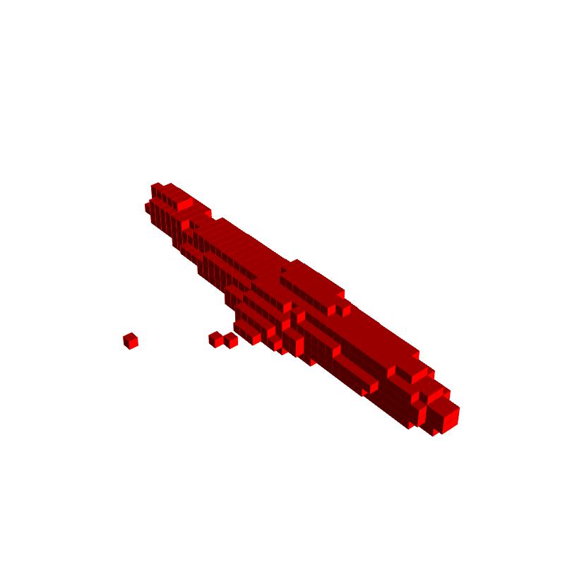
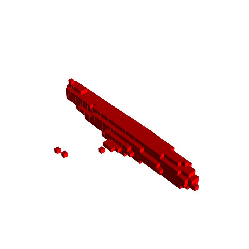
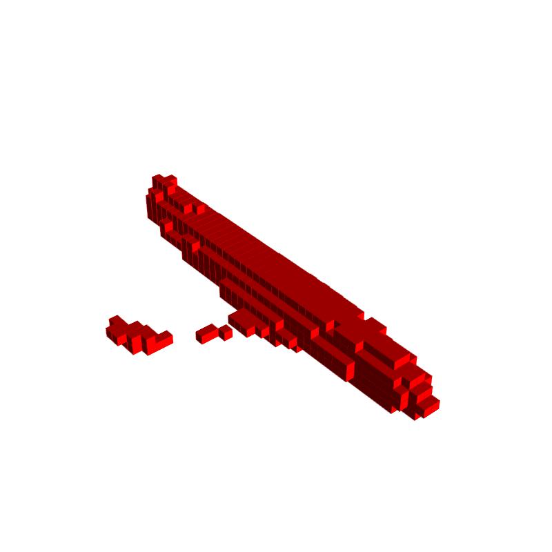
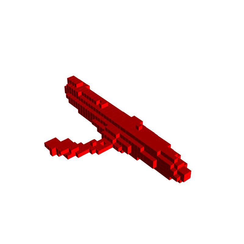
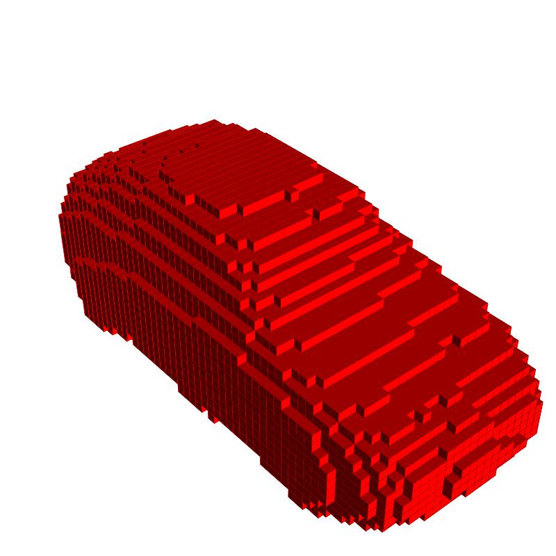
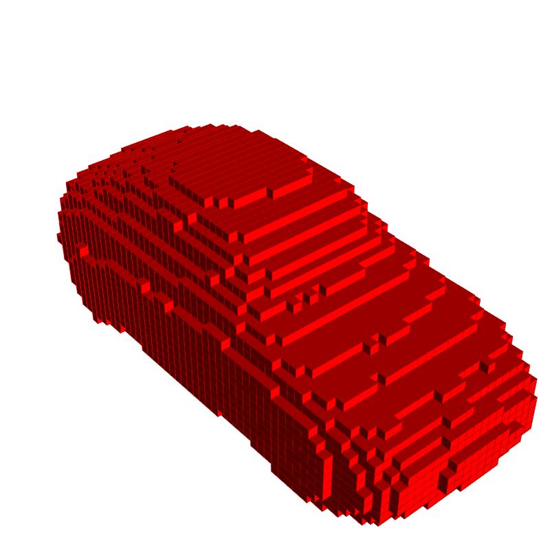
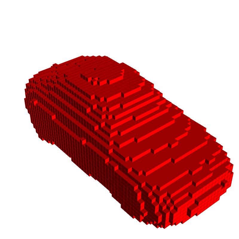
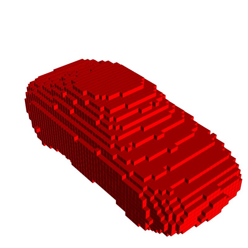
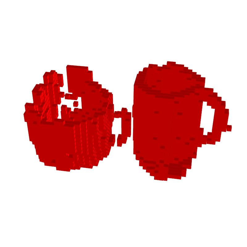
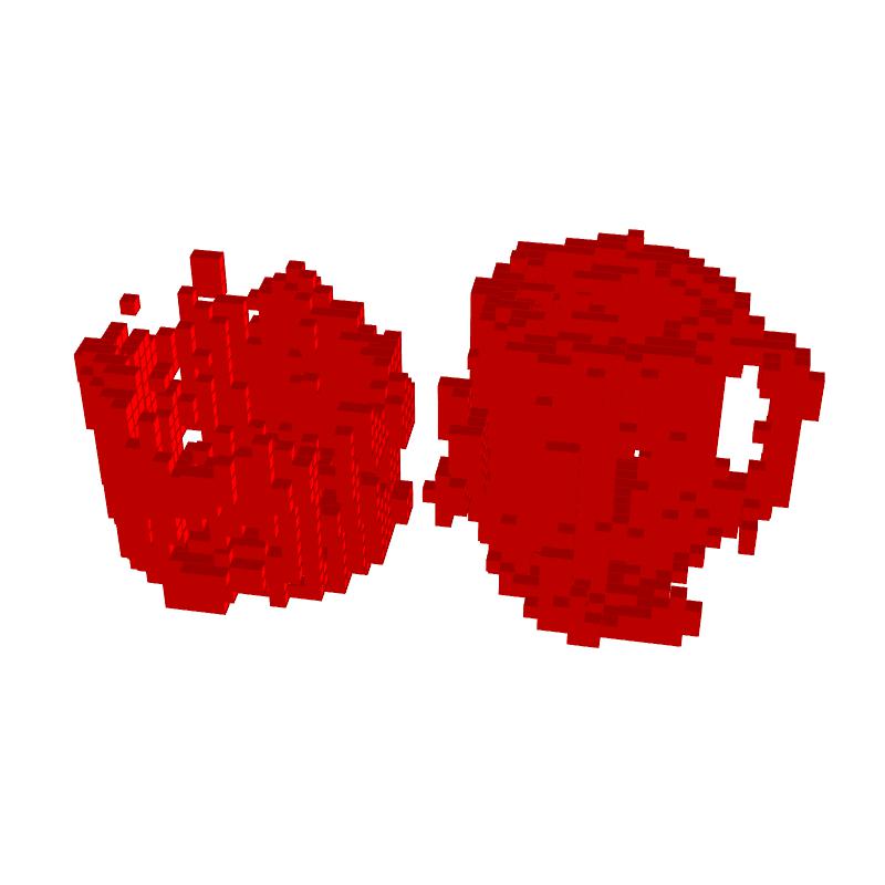
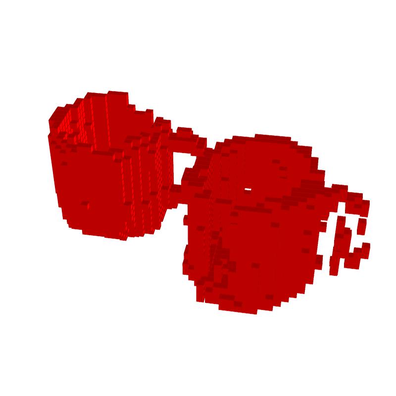
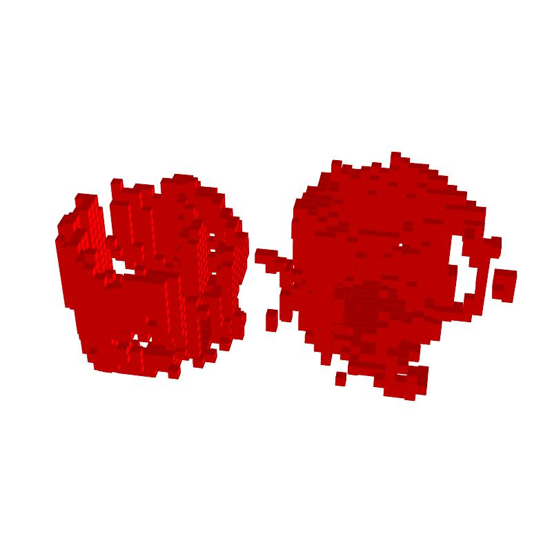
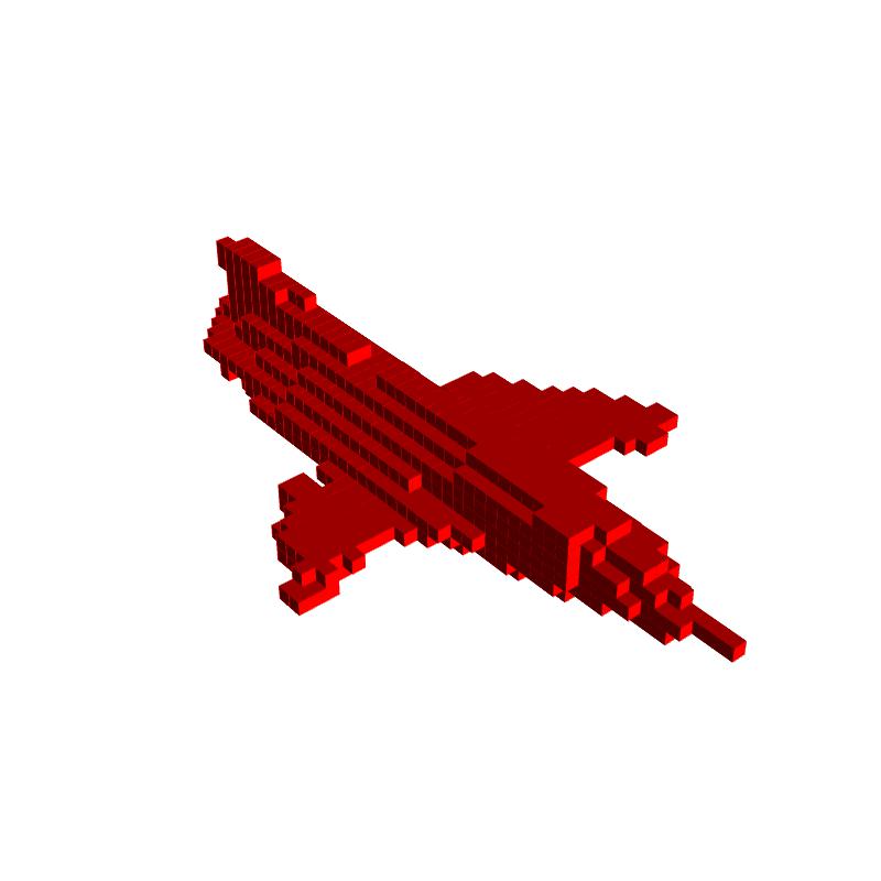
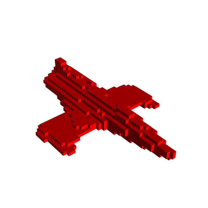
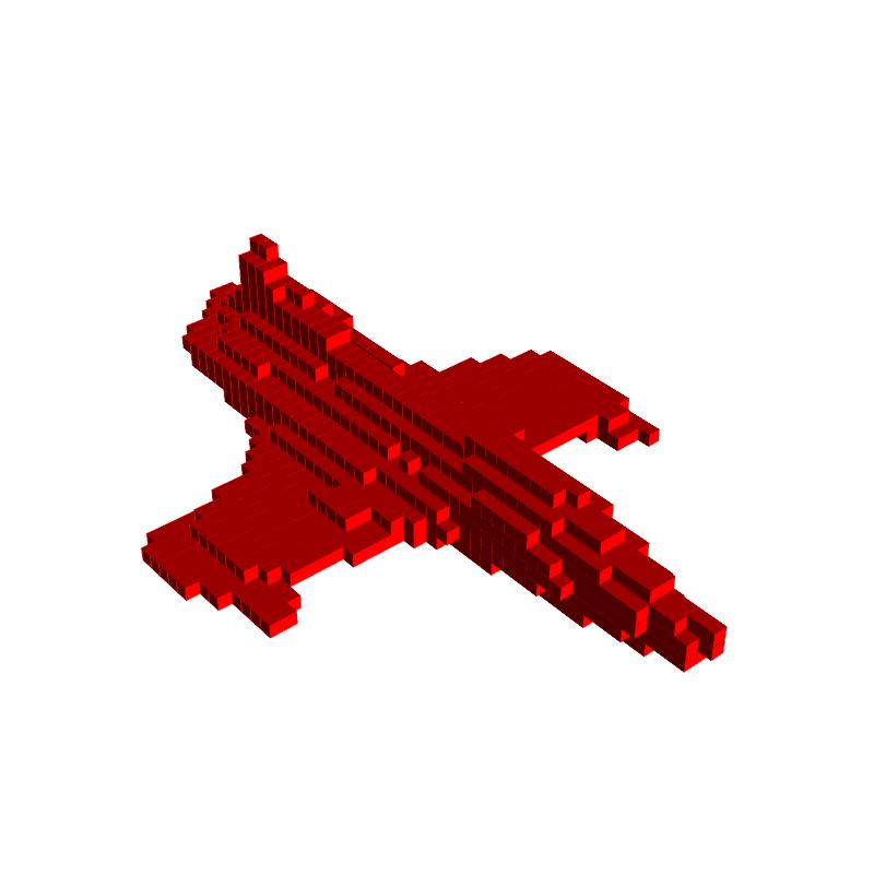
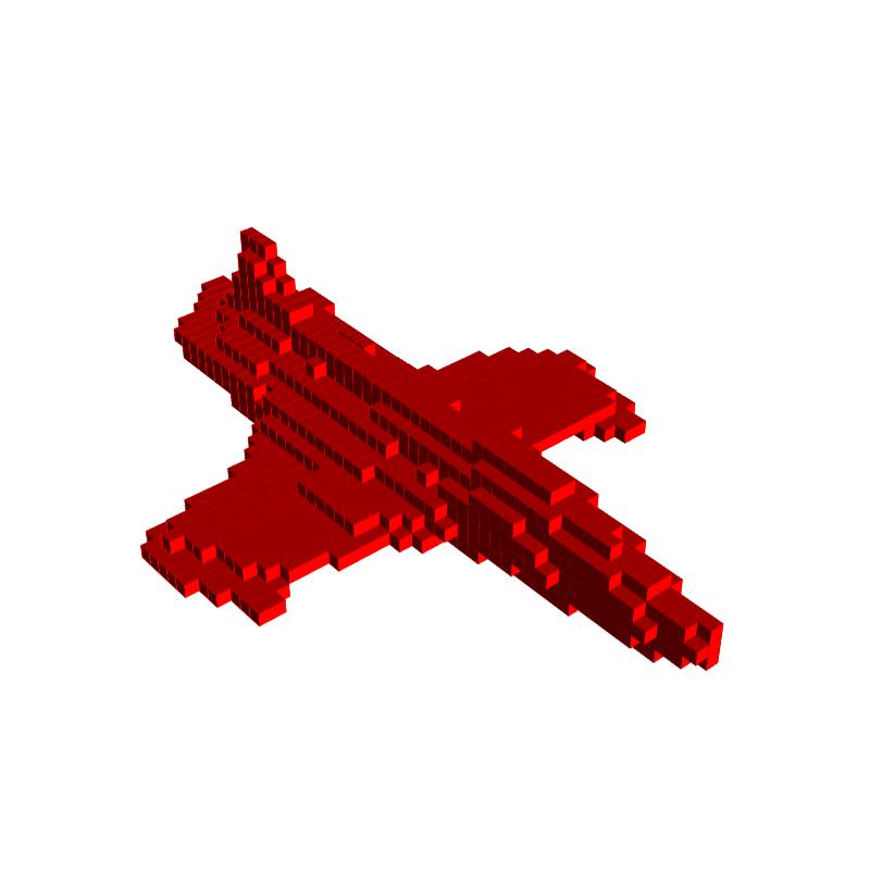
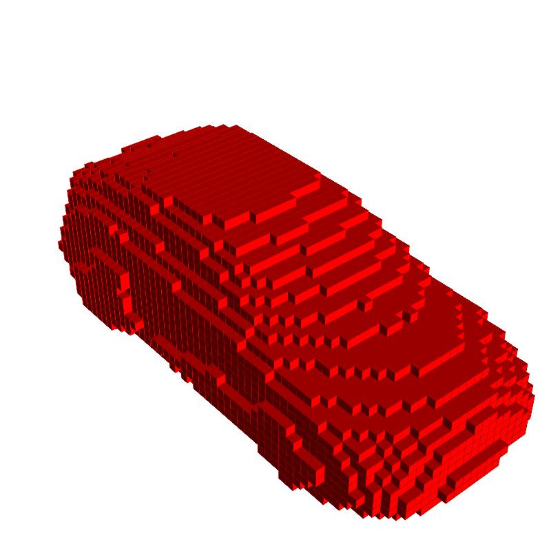
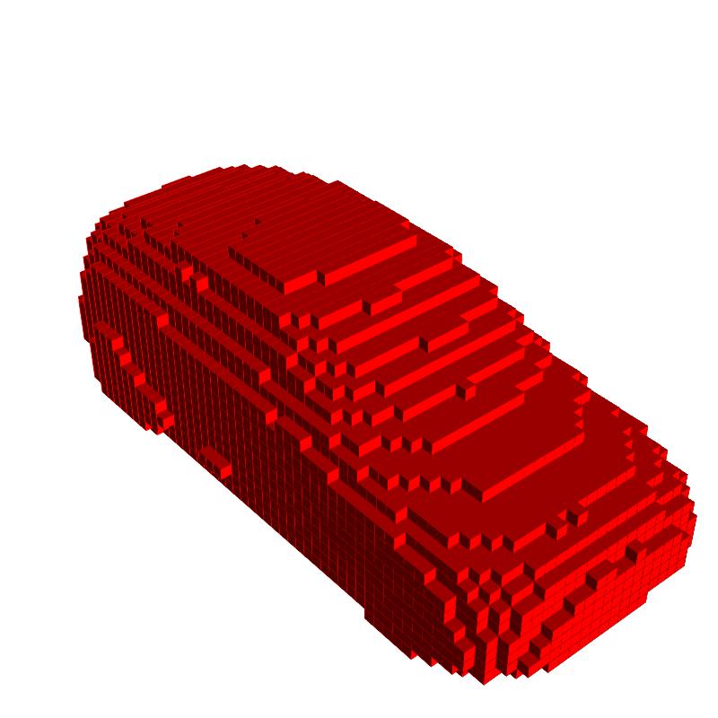
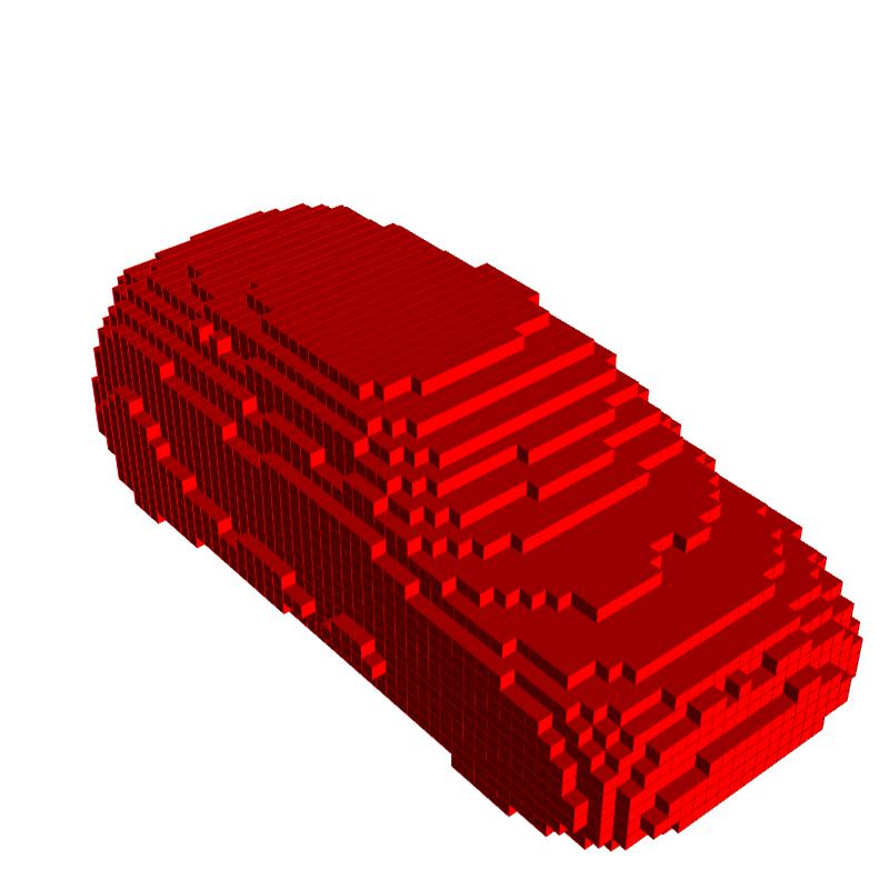
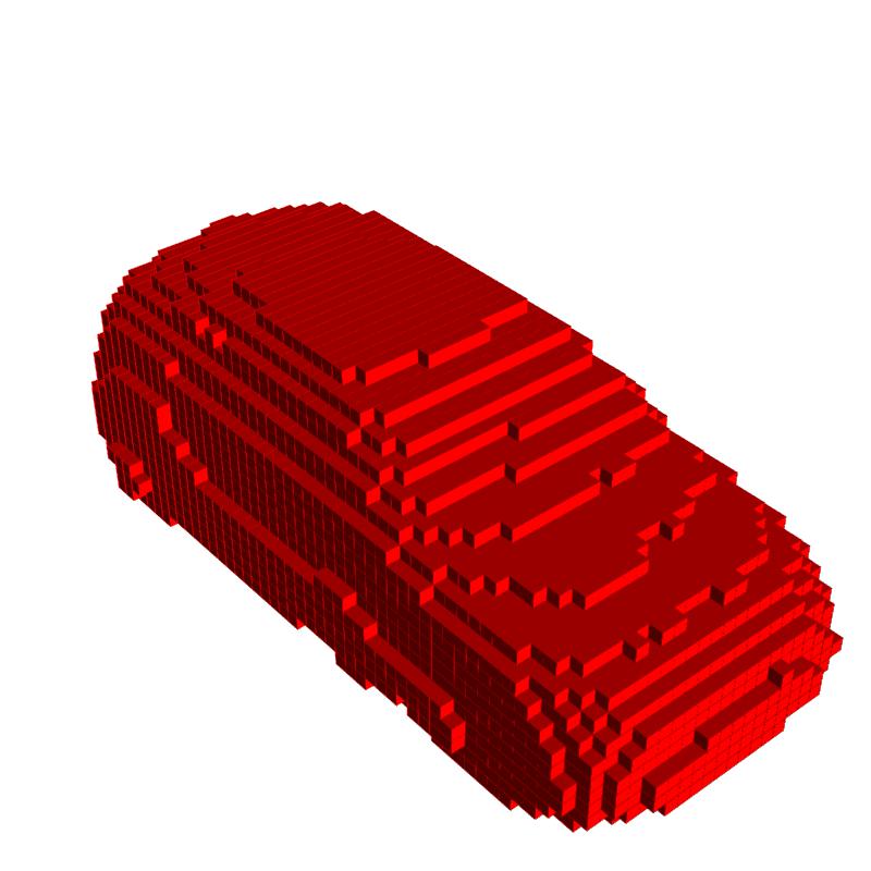
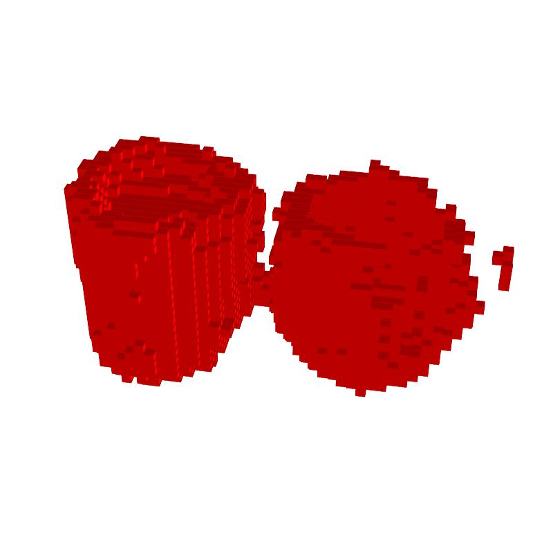
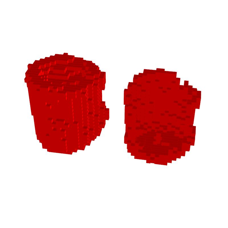
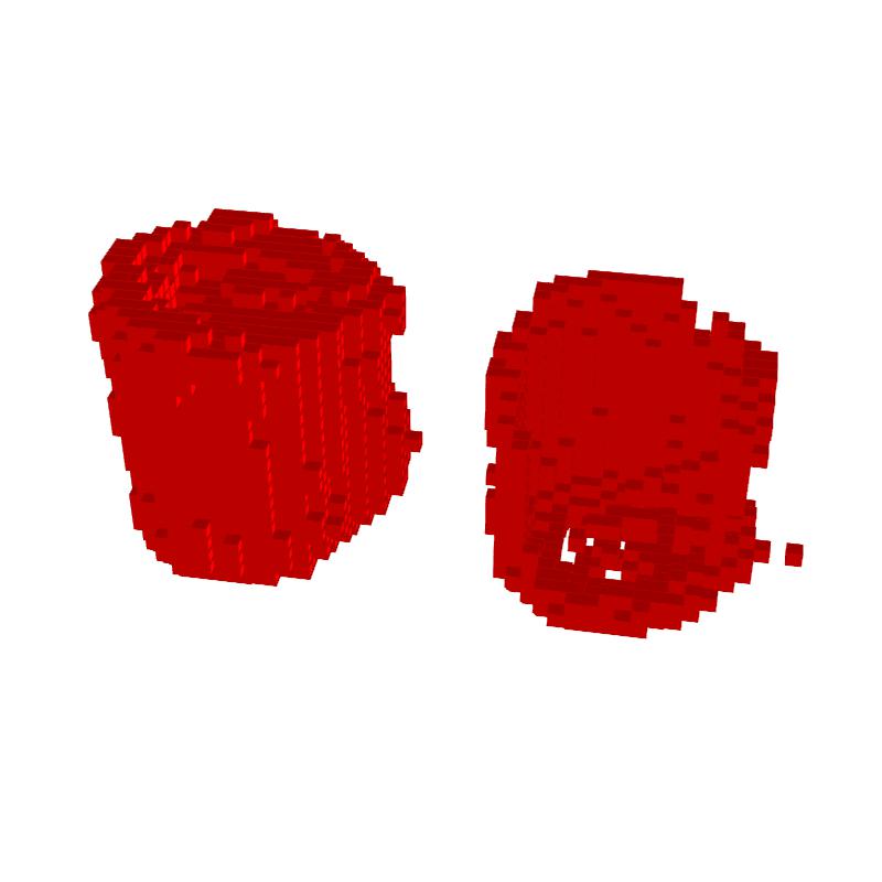
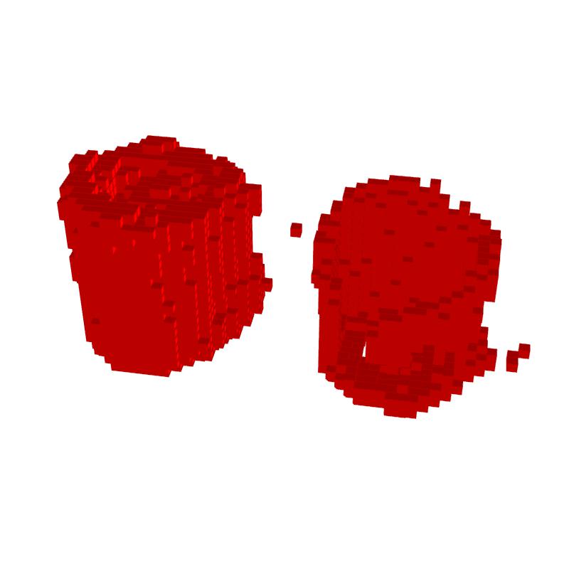
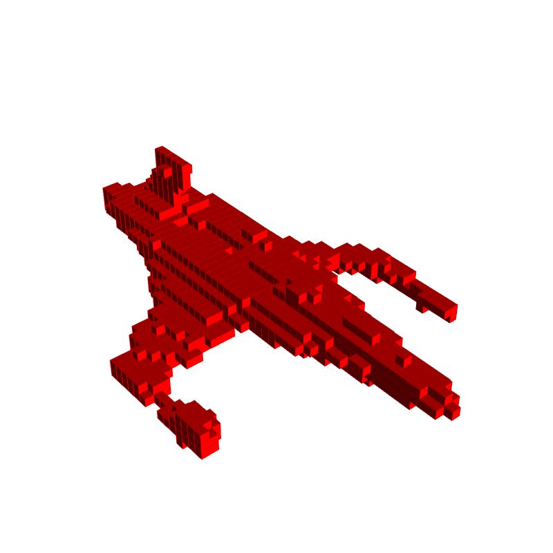
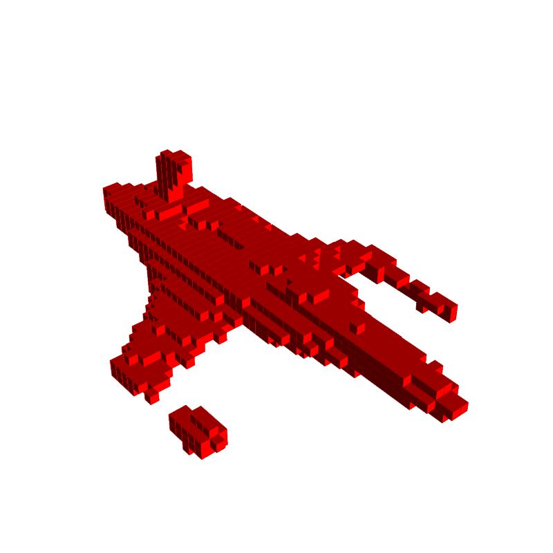
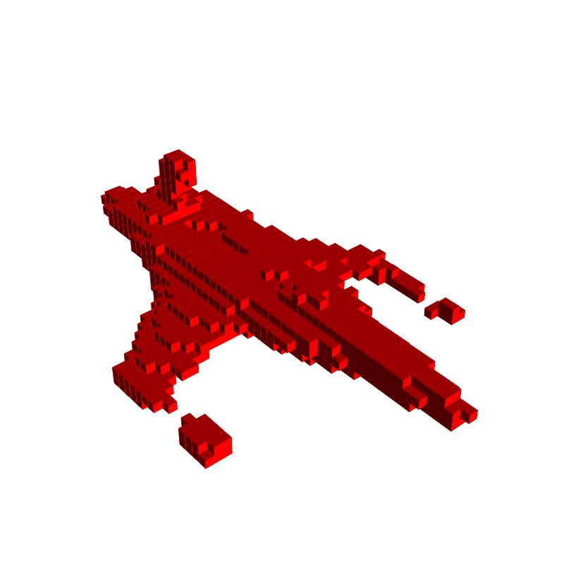
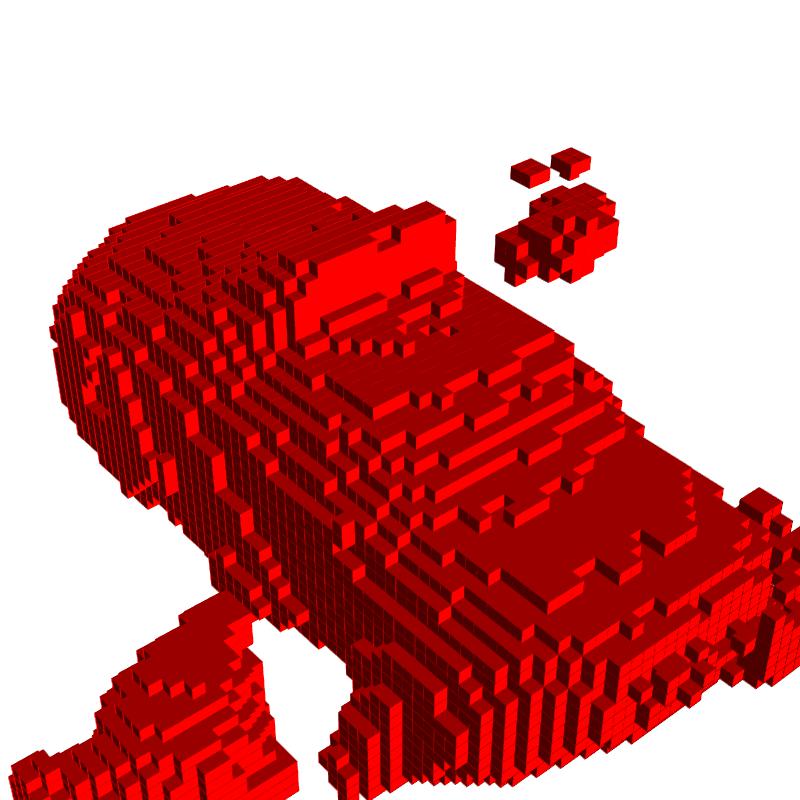
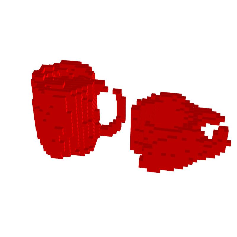
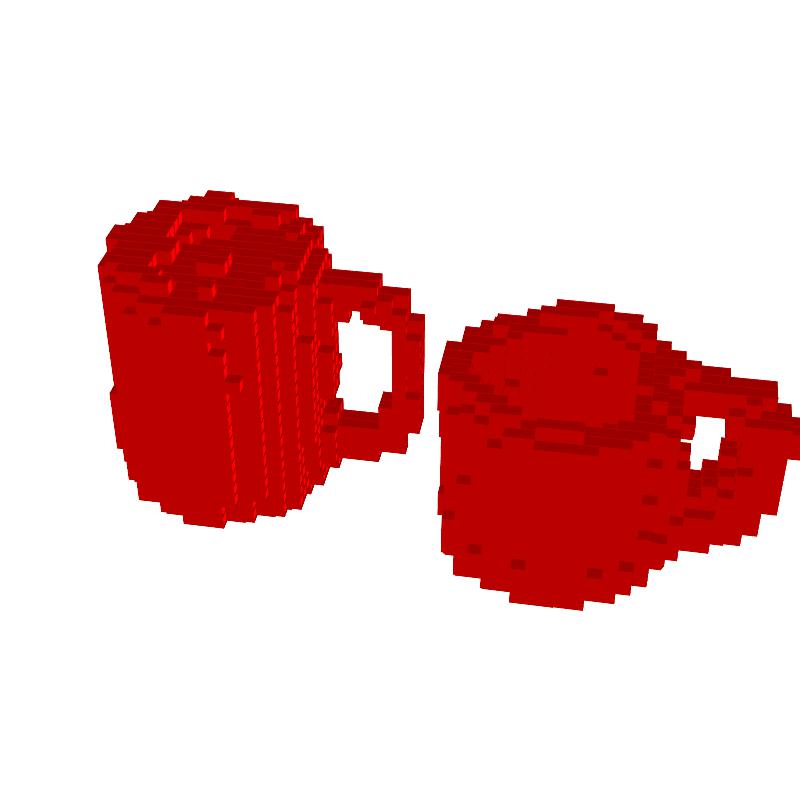
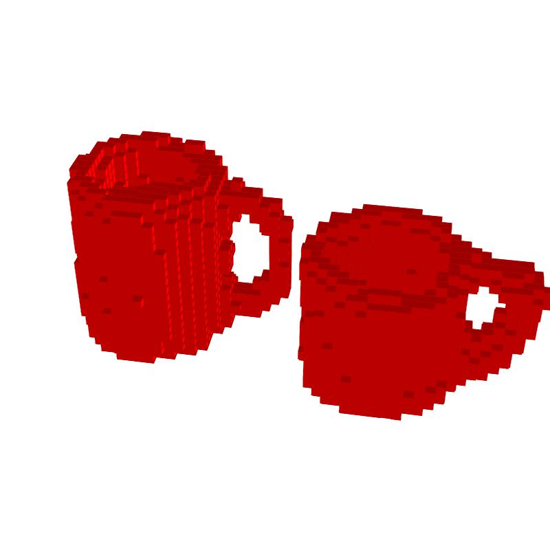
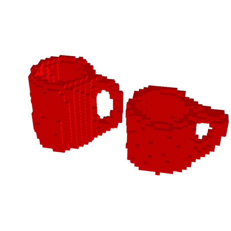
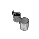
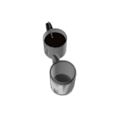
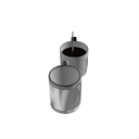
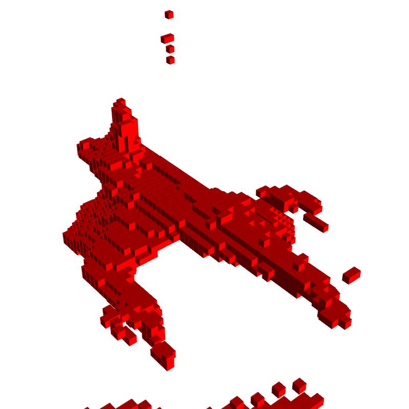
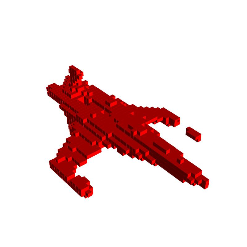
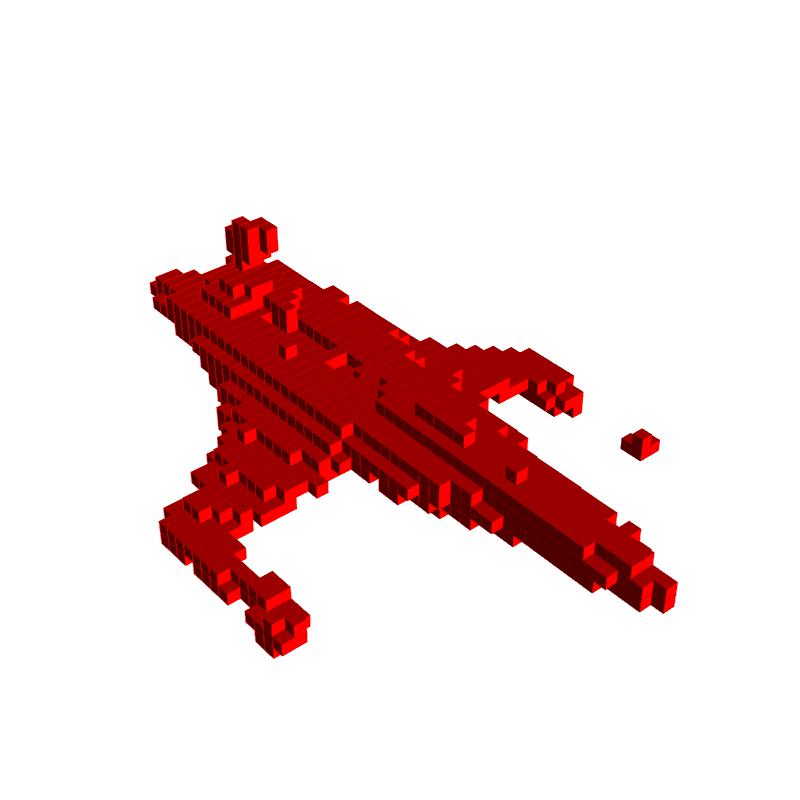
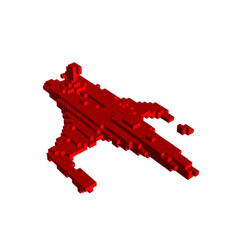
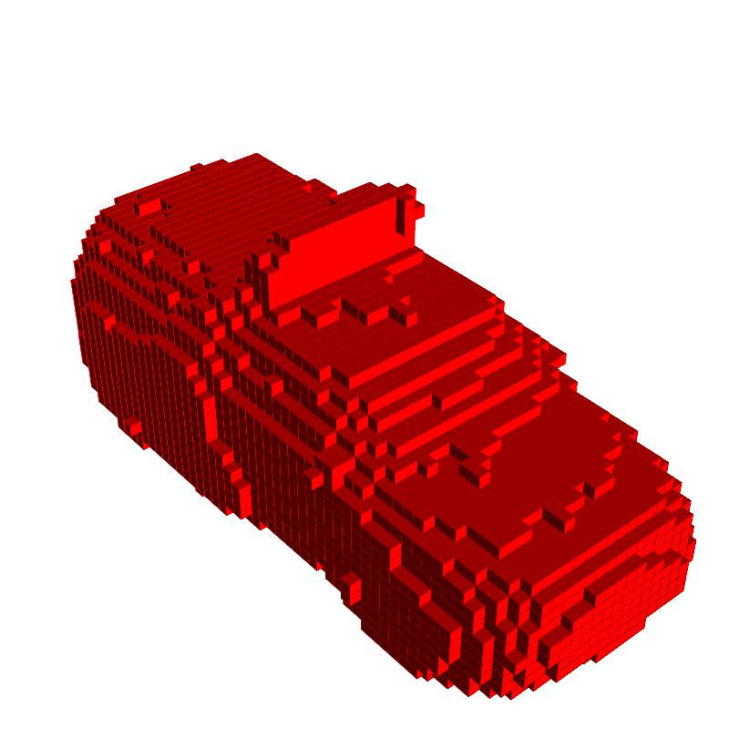
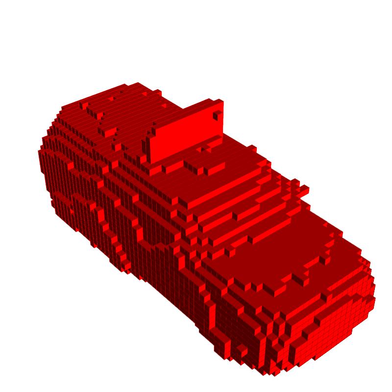
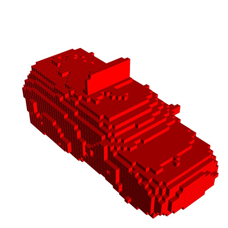
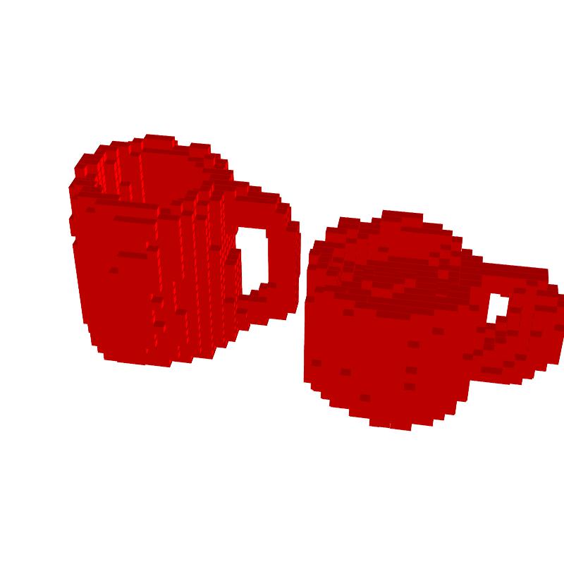
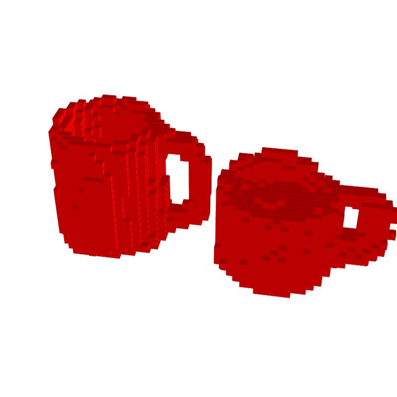
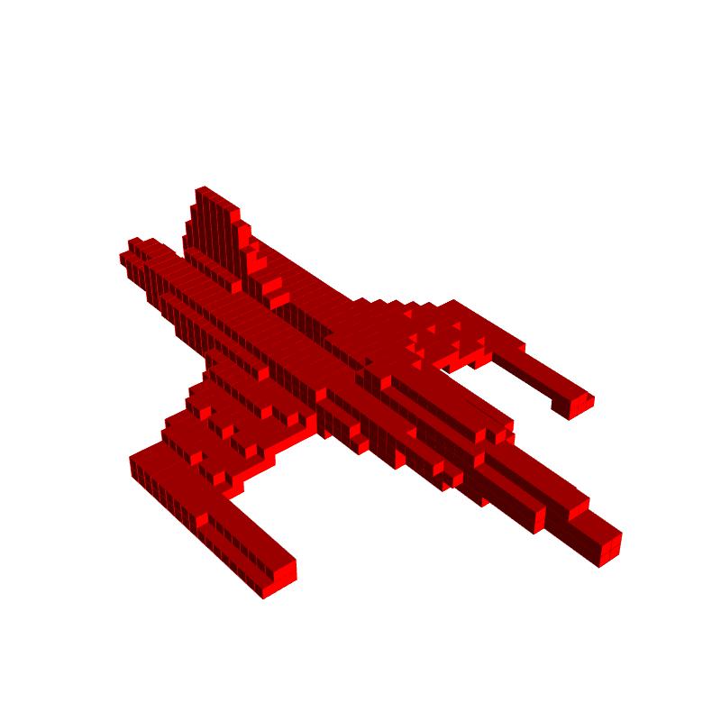
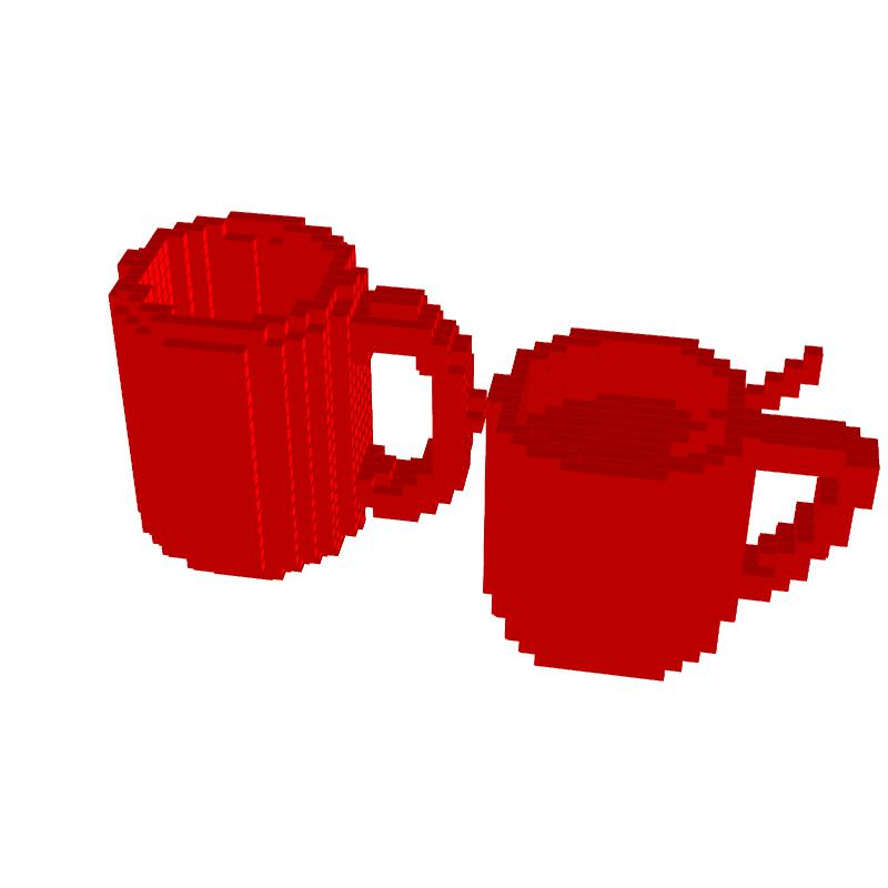
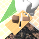
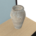
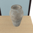
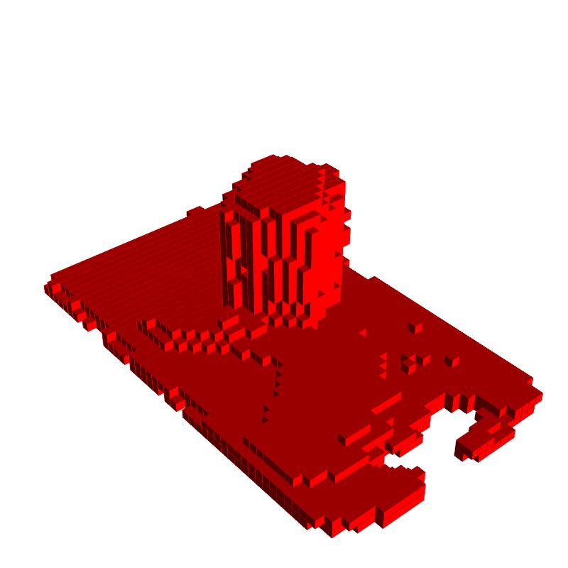
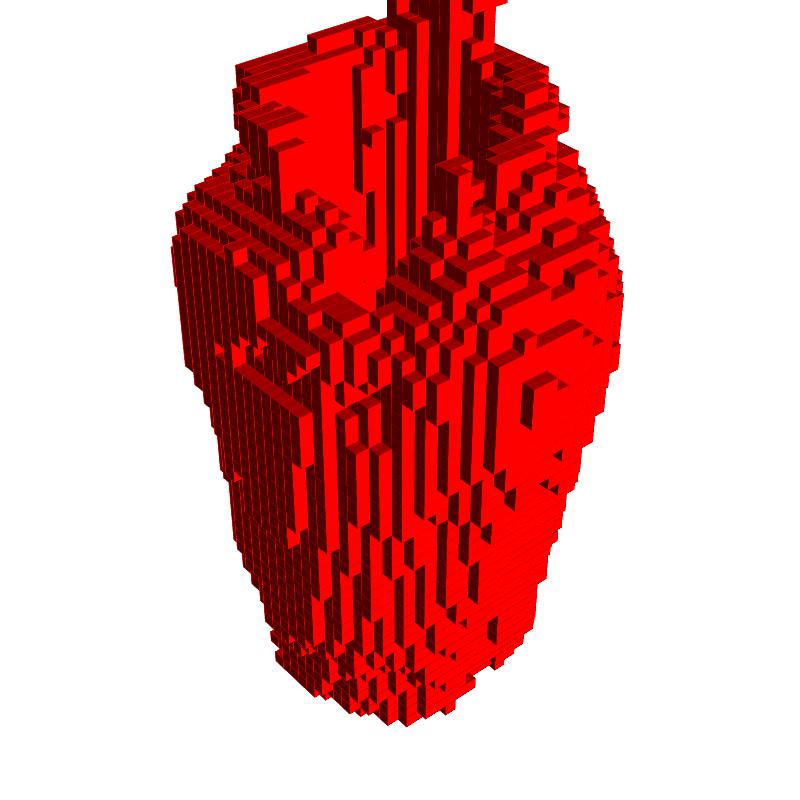
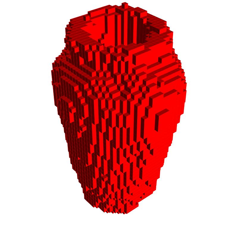
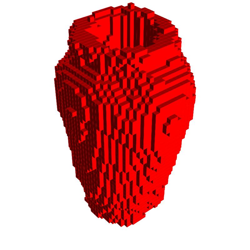
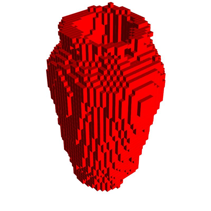
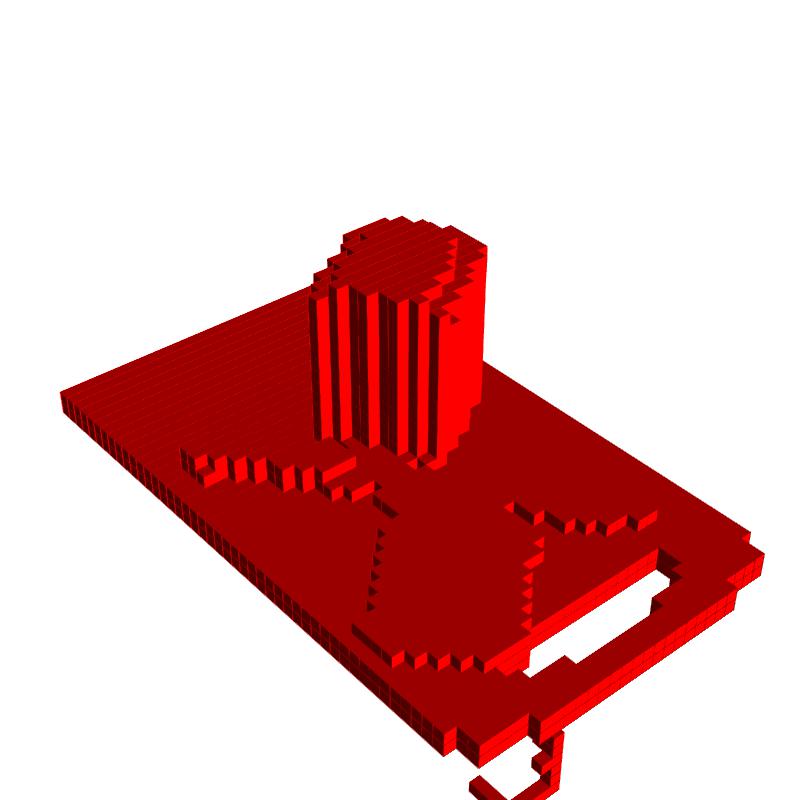
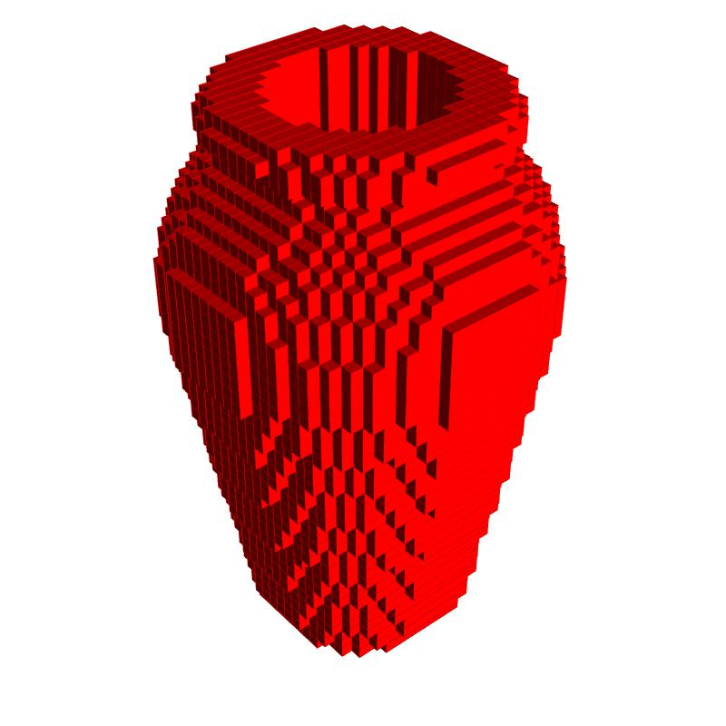
Multi-view reconstruction and 3D segmentation

Here we add more visualization results of reconstruction and 3D segmentation in Figure 4 and Figure 5. In Figure 6, we also included some results of 3D reconstruction on scenes sampled from SUNCG dataset. For data preparation on SUNCG dataset, We first split the house models provided in SUNCG into train and validation set. Then we sample scenes and voxel occupancy from those house models to create data for training and testing.