Global climate modeling of Saturn’s atmosphere.
Part II: multi-annual high-resolution dynamical simulations
Highlights
-
•
A new Global Climate Model for Saturn with radiative transfer
-
•
High-resolution numerical simulations on a duration of 15 Saturn years
-
•
Results on zonal jets, waves, eddies in Saturn’s troposphere
Abstract
The Cassini mission unveiled the intense and diverse activity in Saturn’s atmosphere: banded jets, waves, vortices, equatorial oscillations. To set the path towards a better understanding of those phenomena, we performed high-resolution multi-annual numerical simulations of Saturn’s atmospheric dynamics. We built a new Global Climate Model [GCM] for Saturn, named the Saturn DYNAMICO GCM, by combining a radiative-seasonal model tailored for Saturn to a hydrodynamical solver based on an icosahedral grid suitable for massively-parallel architectures. The impact of numerical dissipation, and the conservation of angular momentum, are examined in the model before a reference simulation employing the Saturn DYNAMICO GCM with a latitude-longitude resolution is considered for analysis. Mid-latitude banded jets showing similarity with observations are reproduced by our model. Those jets are accelerated and maintained by eddy momentum transfers to the mean flow, with the magnitude of momentum fluxes compliant with the observed values. The eddy activity is not regularly distributed with time, but appears as bursts; both barotropic and baroclinic instabilities could play a role in the eddy activity. The steady-state latitude of occurrence of jets is controlled by poleward migration during the spin-up of our model. At the equator, a weakly-superrotating tropospheric jet and vertically-stacked alternating stratospheric jets are obtained in our GCM simulations. The model produces Yanai (Rossby-gravity), Rossby and Kelvin waves at the equator, as well as extratropical Rossby waves, and large-scale vortices in polar regions. Challenges remain to reproduce Saturn’s powerful superrotating jet and hexagon-shaped circumpolar jet in the troposphere, and downward-propagating equatorial oscillation in the stratosphere.
1 Introduction
It has been decades since Saturn’s meteorological phenomena observed by Earth-based and space telescopes, and the pioneering Voyager missions, are challenging the fundamental knowledge of geophysical fluid mechanics (e.g., Ingersoll,, 1990; Dowling,, 1995). Yet, a mission as richly instrumented as Cassini (Porco et al.,, 2005), offering from 2004 to 2017 an unprecedented spatial and seasonal coverage of Saturn’s weather layer, brought a new impulse to the studies of giant planets’ atmospheric dynamics (e.g., review papers by Del Genio et al.,, 2009; Showman et al., 2018a, ).
In Saturn’s troposphere, the Cassini measurements confirmed the banded structure of alternating westward (retrograde) and eastward (prograde) jets, which features a m s-1 super-rotating equatorial jet (Porco et al.,, 2005; García-Melendo et al.,, 2010; Studwell et al.,, 2018). Furthermore, the Cassini instruments assessed the remarkable stability of the enigmatic hexagonal jet in the northern polar region (Baines et al.,, 2009; Sánchez-Lavega et al.,, 2014; Antuñano et al.,, 2015; Fletcher et al.,, 2018), with exquisite details on the structure of the turbulent polar vortex (Sayanagi et al.,, 2017; Baines et al.,, 2018). They also offered a detailed record of mid-latitude convective storms (Dyudina et al.,, 2007; del Río-Gaztelurrutia et al.,, 2012) and vortices (Vasavada et al.,, 2006; Dyudina et al.,, 2008; Trammell et al.,, 2016; del Río-Gaztelurrutia et al.,, 2018), including a chain of infrared bright spots named the “String of Pearls” (Sayanagi et al.,, 2014) and an exceptional coverage of Saturn’s latest Great White Spot (Fischer et al.,, 2011; Sánchez-Lavega et al.,, 2011; Sayanagi et al.,, 2013). Cassini observations of Saturn’s cloud layer was also employed to demonstrate the high rate of conversion of energy from eddies to jets (Del Genio et al.,, 2007; Del Genio and Barbara,, 2012), to detail the structure of vorticity (Read et al., 2009a, ), and to explore Jupiter’s and Saturn’s atmospheric energetic spectra across spatial scales (Galperin et al.,, 2014; Young and Read,, 2017), confirming pre-Cassini theoretical studies about geostrophic turbulence and the inverse energy cascade (Sukoriansky et al.,, 2002). All those observations strongly suggest that large-scale tropospheric banded jets emerge from forcing by smaller-scale eddies and waves arising from hydrodynamical instabilities.
In Saturn’s stratosphere, not only the Cassini instruments led to key discoveries, but the longevity of the mission permitted a seasonal monitoring of the unveiled phenomena. Cassini’s highlights in atmospheric science for the stratosphere include a spectacular stratospheric warming associated with the 2010 Great White Spot (Fletcher et al., 2011b, ; Fletcher et al.,, 2012; Fouchet et al.,, 2016), an equatorial oscillation of temperature in Saturn’s stratosphere (Fouchet et al.,, 2008; Guerlet et al.,, 2011; Li et al.,, 2011) with semi-annual periodicity (Orton et al.,, 2008; Guerlet et al.,, 2018), and a seasonal monitoring of the meridional distribution of Saturn’s stratospheric hydrocarbons (Guerlet et al.,, 2009, 2010; Sinclair et al.,, 2013; Fletcher et al.,, 2015; Sylvestre et al.,, 2015; Guerlet et al., 2015b, ), hinting at a possible interhemispheric transport of chemical species. Cassini measurements even enabled to link a disruption in the downward propagation of the equatorial oscillation to the 2010 Great White Spot occurrence (Fletcher et al.,, 2017). Analogies can be drawn between Saturn’s and the Earth’s stratospheres (Dowling,, 2008). Saturn’s equatorial oscillation is reminiscent of Earth’s Quasi-Biennal Oscillation and Semi-Annual Oscillation (Andrews et al.,, 1987; Baldwin et al.,, 2001; Lott and Guez,, 2013; Guerlet et al.,, 2018), driven by the propagation and breaking of Rossby, Kelvin and inertio-gravity waves. The interhemispheric transport of chemical species, which may affect the hydrocarbons distribution, might be analogous to the Earth’s Brewer-Dobson circulation (Butchart,, 2014).
In this stimulating observational context, new modeling efforts are needed to broaden the knowledge of Saturn’s atmospheric dynamics by demonstrating the mechanisms underlying the above-mentioned observed phenomena. A great deal of past modeling work focused on the processes responsible for the banded tropospheric jets. A major difficulty with a giant planet is that the depth at which the atmosphere merges with the internal dynamo region and the strength at which the atmospheric circulations couple with magnetic disturbances have remained poorly constrained by observations (Ingersoll,, 1990; Liu et al.,, 2008) until gravity measurements were recently performed on board Juno and Cassini (Kaspi,, 2013; Galanti and Kaspi,, 2017; Kaspi et al.,, 2018; Galanti et al.,, 2019). Two distinct modeling approaches have been adopted to account for Saturn’s tropospheric jets: “shallow-forcing” climate models [see next paragraph for references] account for processes in the weather layer (baroclinic instability, moist convective storms), while “deep-forcing” dynamo-like models (Heimpel et al.,, 2005; Yano et al.,, 2005; Kaspi et al.,, 2009; Heimpel and Gómez Pérez,, 2011; Gastine et al.,, 2014; Heimpel et al.,, 2016; Cabanes et al.,, 2017) resolve convection throughout gas giants’ molecular envelopes. Contrary to deep models, shallow climate models have had difficulties reproducing gas giants’ equatorial super-rotating jets. This has been overcome by including either bottom drag and intrinsic heat fluxes to simulate deep interior phenomena (Lian and Showman,, 2008; Schneider and Liu,, 2009; Liu and Schneider,, 2010), or latent heating by moist convective storms (Lian and Showman,, 2010), although the simulated equatorial jets are still about twice as less strong in simulations than in observations (e.g., García-Melendo et al.,, 2010). The situation for off-equatorial jets is reversed, with better agreement with observations obtained by shallow models compared to deep models, although the latter can be modified to obtain more realistic results (Heimpel et al.,, 2005). The recent results from the Juno mission for Jupiter (Kaspi et al.,, 2018; Guillot et al.,, 2018) and the Cassini mission for Saturn (Galanti et al.,, 2019) show that banded jets extend several thousand kilometers below the cloud layer, i.e. deeper than what shallow models consider and shallower than what deep models consider, which probably indicates that shallow and deep models have both their virtues to represent part of the reality.
Here we adopt the approach of “shallow-forcing” climate modeling to study Saturn. In the last decade, the traditional approach using idealized modeling (Cho and Polvani,, 1996; Williams,, 2003; Vasavada and Showman,, 2005) – which still has great value to study how baroclinic and barotropic instabilities shape Saturn’s jets (Li et al.,, 2006; Kaspi and Flierl,, 2007; Showman,, 2007), including its polar hexagonal jet (Rostami et al.,, 2017) and central vortex (O’Neill et al.,, 2015) – has been complemented by the development of complete three-dimensional Global Climate Models (GCMs) for Saturn and giant planets (Dowling et al.,, 1998, 2006; Lian and Showman,, 2010; Liu and Schneider,, 2010; Young et al., 2019a, ; Young et al., 2019b, ). A GCM is obtained by coupling a hydrodynamical solver of the Navier-Stokes equations for the atmospheric fluid on the sphere (the GCM’s “dynamical core”) with realistic models for physical processes operating at unresolved scales: radiation, turbulent mixing, phase changes, chemistry (the GCM’s “physical packages”). Most of those existing GCM studies for Saturn address the formation of tropospheric jets by angular momentum transfer through eddies and waves, often with either a theoretical approach aiming to address giant planets’ atmospheric dynamics (Schneider and Liu,, 2009; Lian and Showman,, 2010; Liu and Schneider,, 2010, 2015) rather than a focused approach aiming to address Saturn specifically, or with a limited-domain approach using a latitudinal channel enclosing one specific jet to explain structures such as the Ribbon wave or the String of Pearls (Sayanagi et al.,, 2010, 2014), to investigate the impact of convective outbursts (Sayanagi and Showman,, 2007; García-Melendo et al.,, 2013), or to discuss the polar hexagonal jet (Morales-Juberías et al.,, 2011, 2015). The idealized GCM approach can also be employed to study equatorial oscillations in gas giants (Showman et al., 2018b, ). All those existing studies use simple radiative forcing rather than computing a realistic “physical package” that includes seasonally-varying radiative transfer. The latter approach has been explored to study Saturn’s stratosphere, either to constrain large-scale advection / eddy mixing in photochemical models (Friedson and Moses,, 2012), or to build a modeling framework applicable to extrasolar hot gas giants (Medvedev et al.,, 2013). Those studies of Saturn’s stratosphere make use, however, of prescribed, ad hoc, tropospheric jets.
The existing body of work on “shallow-forcing” modeling has thus paved the path towards a complete three-dimensional Global Climate Model (GCM) for giant planets. However, such a complete troposphere-to-stratosphere GCM for Saturn, capable to address the theoretical challenges opened by observations is yet to emerge. We propose that four challenges shall be overcome to develop a complete state-of-the-art GCM for Saturn and gas giants.
-
The radiative transfer computations necessary to predict the evolution of atmospheric temperature, especially in the stratosphere, must be optimized for integration over decade-long giant planets’ years, while still keeping robustness against observations.
-
Large-scale jets and vortices emerge from smaller-scale hydrodynamical eddies, through an inverse energy cascade driven by geostrophic turbulence. Relevant interaction scales (e.g. Rossby deformation radius) are only latitude-longitude in gas giants vs. on the Earth, making eddy-resolving global simulations over a full year four orders of magnitude more computationally expensive in gas giants.
-
Terrestrial experience shows that models need to extend from the troposphere to the stratosphere with sufficient vertical resolution to resolve the vertical propagation of waves responsible for large-scale structures in both parts of the atmosphere. Moreover, a specific requirement of giant planets is to extend the model high enough in the stratosphere to model the photochemistry of key hydrocarbons impacting stratospheric temperatures (Hue et al.,, 2016).
-
Climate models cannot extend neither deep enough to predict how tropospheric jets interact with interior convective fluxes and planetary magnetic field (Kaspi et al.,, 2009; Heimpel and Gómez Pérez,, 2011), nor high enough to capture the coupling of stratospheric circulations with thermospheric and ionospheric processes (Müller-Wodarg et al.,, 2012; Koskinen et al.,, 2015). A suitable approach to couple the weather layer with either the slowly-evolving convective interior, or the rapidly-evolving ionized external layers, remains elusive.
Here we report the development and preliminary dynamical simulations of a new Saturn GCM at Laboratoire de Météorologie Dynamique (LMD), which aims at understanding the seasonal variability, large-scale circulations, and eddy & wave activity in Saturn’s troposphere and stratosphere. It is a first step to further design a modeling platform dedicated to atmospheric circulations of Saturn and other solar system’s giant planets. Challenge about building fast and accurate radiative transfer for the Saturn GCM is addressed in Guerlet et al., (2014). In Guerlet et al., (2014), which serves as Part I for the present study, a seasonal radiative–convective model of Saturn’s upper troposphere and stratosphere is described and the sensitivity to composition, aerosols, internal heat flux and ring shadowing is assessed, with comparisons to the observed thermal structure by Cassini and ground-based telescopes. In this Part II paper, we address Challenge by performing high-resolution dynamical simulations with our Saturn GCM. Our GCM is built by coupling the physical packages (notably, radiative transfer) of Guerlet et al., (2014) with DYNAMICO, a new dynamical core developed at LMD which uses an original icosahedral mapping of the planetary sphere to ensure excellent conservation and scalability properties in massively parallel resources (Dubos et al.,, 2015). We describe here the insights gained from GCM simulations at high horizontal resolutions (reference at latitude/longitude, and tests at and ) with two unprecedented characteristics at those horizontal resolutions: inclusion of realistic radiative transfer and long integration times up to fifteen simulated Saturn years.
The paper is organized as follows. Notations are defined in Table 1. In section 2, we provide details on the characteristics of our Saturn DYNAMICO GCM, and the assumptions and settings adopted for the simulations discussed in subsequent sections, with appendix A featuring a necessary analysis of the impact of horizontal dissipation and the conservation of angular momentum in our Saturn GCM. In section 3, we describe the results obtained with our reference 15-year-long Saturn DYNAMICO GCM simulation, with an emphasis on the driving and evolution of jets in section 4. In section 5, we summarize our conclusions and draw perspectives for future improvements of our Saturn DYNAMICO GCM needed to fully achieve challenges , and , as it comes to no surprise that the present study is only a preliminary path towards fulfilling arguably ambitious scientific goals.
| Coordinates | ||
|---|---|---|
| Time | s | |
| Longitude, Latitude | ∘E, ∘N | |
| WE coordinate, SN coordinate (local frame) | m | |
| Altitude | m | |
| Saturn’s heliocentric longitude ( N spring) | ∘ | |
| Meteorological variables | ||
| Pressure | Pa | |
| Temperature | K | |
| Zonal wind component (W E) | m s-1 | |
| Meridional wind component (S N) | m s-1 | |
| Vertical wind component | m s-1 | |
| Atmospheric mass | kg | |
| Axial Angular Momentum (AAM) | kg m2 s-1 | |
| Specific AAM (per unit mass, equation 18) | m2 s-1 | |
| Relative vorticity (vertical component ) | m s-2 | |
| Ertel potential vorticity | kg m2 s-1 K-1 | |
| Planetary parameters and model settings | ||
| Rotation rate⋆ | s-1 | |
| Obliquity | ||
| Acceleration of gravity | m s-2 | |
| Planetary radius | m | |
| Specific heat capacity | J kg-1 K-1 | |
| Molecular mass | g mol-1 | |
| Ideal gas constant normalized with | ||
| Internal heat flux | W m-2 | |
| Timescale for bottom Rayleigh drag | 100 Earth days | |
| Minimum latitude () for bottom drag | ||
| Computations | ||
| Coriolis parameter at latitude | s-1 | |
| Beta parameter (meridional derivative of ) | m-1 s-1 | |
| Atmospheric scale height | m | |
| Brunt-Väisälä frequency | s-2 | |
| Axisymmetric component of variable | Zonal average | |
| Eddy† component of variable | Zonal anomaly | |
⋆ The rotation rate corresponds to Saturn “days” of s, according to the value obtained in Read et al., 2009b using an approach based on potential vorticity (denoted System IIIw).
† Eddies are defined as deviations (perturbations) from the zonal-mean flow and can represent the effects of turbulence, waves, and instabilities.
2 Characteristics of the Saturn DYNAMICO GCM
2.1 Building the model
As is reminded in the introduction, a GCM consists in coupling a dynamical core interfaced with physical packages (or parameterizations). Our project to develop a Saturn GCM started by the development of the latter: the physical packages used in our GCM are described in full detail in Guerlet et al., (2014). Our model’s radiative computations are based on a versatile correlated- method, suitable for any planetary composition (Wordsworth et al.,, 2010; Charnay et al.,, 2013; Leconte et al.,, 2013) with -coefficients derived from detailed line-by-line computations using the HITRAN spectroscopic database (Rothman et al.,, 2013). Radiative contributions include the three main hydrocarbons (methane, ethane and acetylene), the broad H2-H2 and H2-He collision-induced absorption (Wordsworth,, 2012), and tropospheric and stratospheric aerosols layers. Our radiative computations also feature ring shadowing (appendix A in Guerlet et al.,, 2014) and account for internal heat flux independent with latitude (section 2 in Guerlet et al.,, 2014).
The spectral discretization of the correlated- model is optimized for Saturn, with a particular emphasis on accounting for absorption and emission bands of stratospheric methane CH4 (the prominent driver of Saturn’s stratospheric heating), and other hydrocarbons produced by its photodissociation (ethane C2H6 and acetylene C2H2, the prominent drivers of Saturn’s stratospheric cooling). Compared to Guerlet et al., (2014), the line list for methane has been updated beyond 9200 cm-1 (Rey et al.,, 2018, in lieu of the Karkoschka and Tomasko, (2010) band model) and the two main isotopes 13CH4 and CH3D are now included. This improves the predicted temperatures in the middle stratosphere ( mbar) by about K. The vertical profiles of hydrocarbons’ abundances are held constant with latitude and season, and set as is described in Guerlet et al., (2014) using a combination of Cassini observations (Guerlet et al.,, 2009) and photochemical modeling (Moses et al.,, 2000). Variations up to of acetylene abundance are observed at high latitudes (Fletcher et al.,, 2015, note that Sylvestre et al., (2015) found weaker variations) which would entail temperature variations of a couple K in the vicinity of the 1-mbar level (Guerlet et al.,, 2014, section 4.4); coupling our radiative model with a seasonal photochemical scheme is considered as a future development for dedicated middle-to-upper stratosphere GCM simulations (see Challenge , as well as Hue et al.,, 2016, 2018).
Guerlet et al., (2014) showed that this seasonal model allowed for both efficiency and accuracy, with satisfactory comparisons with Cassini measurements – including the observed temperature “knee” caused by heating at the top of the tropospheric aerosol layer, and the meridional gradient between the summer and winter stratosphere (Fletcher et al., 2010a, ; Fletcher et al.,, 2015). Temperatures predicted with our Saturn DYNAMICO GCM are compared with Cassini measurements in section 3.1.
The need to address specifically Challenge (i.e. to achieve fine-enough horizontal resolutions in order to predict the arising of smaller-scale eddies and the inverse cascade in the context of geostrophic turbulence) requires the use of a suitable dynamical core in our Saturn GCM. To that end, we chose to employ DYNAMICO, which is developed at LMD as the next state-of-the-art dynamical core for Earth and planetary climate studies (Dubos et al.,, 2015), and tailored for massively parallel High-Performance Computing resources (scalability tested up to cores).
Our dynamical core DYNAMICO solves the primitive hydrostatic equations assuming a shallow atmosphere, i.e. (relaxing this assumption to solve the quasi-hydrostatic deep-atmosphere equations is considered for future developments of the model, Tort et al.,, 2015). The global horizontal mesh in DYNAMICO is set as a quasi-uniform icosahedral C-grid (Dubos et al.,, 2015) obtained by subdivision of a regular icosahedron: the total number of hexagonal cells is corresponding to sub-triangles subdividing each of the 10 main triangles of the icosahedron grid ( is the parameter by which the horizontal resolution is set in DYNAMICO). Control volumes for mass, tracers and entropy/potential temperature are the hexagonal cells of the Voronoi mesh to avoid the fast numerical modes of the triangular C-grid. Vertical coordinates are mass-based coordinates: “sigma” levels defined as where is the pressure at the bottom of the model.
Spatial discretizations in DYNAMICO are formulated following an energy-conserving three-dimensional Hamiltonian approach (Dubos et al.,, 2015). Time integration is done by an explicit Runge-Kutta scheme (chosen for stability and accuracy). Subgrid-scale (unresolved) dissipation in the horizontal dimension is included as an additional hyperdiffusion term in the vorticity, divergence and temperature equations (see section A.1). In the vertical dimension, subgrid-scale dissipation is handled in the physical packages through a combination of a Mellor and Yamada, (1982) diffusion scheme for small-scale turbulence, and a dry convective adjustment scheme for organized turbulence (convective plumes, see section 2.4 of Hourdin et al.,, 1993). In the case of our Saturn DYNAMICO GCM simulations, the adjustment scheme is the dominant term enabling a neutral profile in the troposphere. This simple adjustment scheme computes the temperature tendencies required to reach the entropy-conserving mixed layer of any convectively-unstable layer appearing in the model. Those characteristics entail that this scheme is not a source of small-scale eddies in the model, which was checked in practice in our Saturn DYNAMICO GCM.
The XIOS library (XML Input/Output Server, Meurdesoif,, 2012, 2013) is employed to handle any input/output operations independently from the timeframe imposed by the numerical integrations: not only this improves the efficiency of the numerical integrations in massively-parallel computing clusters, but this also enables for complex operations on computed fields to be carried out during model runtime rather than as a post-processing operation. Notably, mapping the dynamical fields computed in the non-conformal icosahedral DYNAMICO grid towards a regular latitude-longitude grid, using finite-volume weighting functions, is performed by XIOS directly during our GCM runtime.
2.2 Model settings and boundary conditions
The simulations discussed in this paper are obtained from integrations with our Saturn DYNAMICO GCM employing an horizontal icosahedral mesh with , corresponding to an approximate horizontal resolution of in longitude/latitude (hereafter simply referred to as “ simulations”). Test simulations with ( simulations) and ( simulations), aimed at model testing rather than scientific exploration, are discussed in section 5 to open perspectives for future work. The integration, dynamical timestep in the Saturn simulations is s. Computations in physical packages are done every 160 dynamical timesteps (i.e. every half a Saturn day) with the exception of radiative computations, which are done every 40 physical timesteps (i.e. every dynamical timesteps, which is every 20 Saturn days). This means that while the radiative tendency of temperature is added to the dynamical integrations at each physical timestep (every half a Saturn day), it is only updated by our radiative package every 20 Saturn days. This is long compared to what is considered standard in GCMs for terrestrial planets, yet compliant with the comparatively long radiative timescales (or, equivalently, weak radiative forcing) in gas giants. As is indicated in Guerlet et al., (2014), typical radiative timescales on Saturn are longer than a Saturn year below the 400-mbar pressure level and still about a third of a Saturn year at the 10-mbar level. This is much longer than the timescales of dynamical phenomena (most notably eddies) resolved in the model. We tested that simulations with smaller radiative timesteps yield similar results as reference simulations; we also checked that the diurnal cycle in radiative tendencies is negligible both in Saturn’s troposphere and stratosphere.
Our simulations feature levels in the vertical dimension, ranging from bars at the model bottom, to mbar at the model top. The Saturn DYNAMICO GCM simulations discussed in this paper thus extend from the lower troposphere to the middle stratosphere. Our model top is too low, and our vertical resolution too coarse in the stratosphere, to address Challenge . This shall be improved in further studies dedicated specifically to Saturn’s stratospheric phenomena (notably, the equatorial oscillation). Our DYNAMICO model features an optional absorbing (“sponge”) layer with a Rayleigh drag acting on the topmost model layers as a surrogate for gravity wave drag in the stratosphere, but we do not use it for the simulations presented in this paper, similarly to previous studies (Schneider and Liu,, 2009; Liu and Schneider,, 2010). Indeed, Shaw and Shepherd, (2007) showed that the inclusion of sponge-layer parameterizations that do not conserve angular momentum (which is the case for Rayleigh drag), or allow for momentum to escape to space, implies a sensitivity of the dynamical results (especially zonal wind speed) to the choice for model top or drag characteristic timescale, because of spurious downward influence when momentum conservation is violated.
Our bottom condition at the -bar level is similar to Liu and Schneider, (2010). We include a simple Rayleigh-like drag , with a timescale Earth days. This drag plays the role devoted to surface friction on terrestrial planets, which allows to close the angular momentum budget through downward control (Haynes and McIntyre,, 1987; Haynes et al.,, 1991). This could also be regarded as a zeroth-order parameterization for Magneto-HydroDynamic (MHD) drag as a result of Lorenz forces acting on jet streams putatively extending to the depths of Saturn’s interior (Liu et al.,, 2008; Galanti et al.,, 2019), much deeper than the shallow GCM’s model bottom. Whether or not including a bottom drag at bars is physically justified is out of the scope of the present paper, and improving on this admittedly simplistic bottom boundary condition is an entire research goal on its own (part of what we named Challenge ). In the present study, we take this bottom drag as an imperfect, yet unambiguous, means to close the angular momentum budget and accounting for deep-seated phenomena in shallow-forcing models for gas giants (Schneider and Liu,, 2009; Liu and Schneider,, 2010, 2015).
Similarly to Liu and Schneider, (2010), the bottom drag is not exerted at equatorial latitudes (i.e. ) as it artificially suppresses the cylindrical barotropic circulation structures that develop along the rotational axis (Taylor columns). This approach mimics the so-called tangent cylinder, which is thought to cause the equatorial super-rotating jets in deep-convective models (Heimpel et al.,, 2005; Kaspi et al.,, 2009). The value is obtained by the geometrical constraint , with km, ie. a depth of km below the 1-bar level. This corresponds to the depths at which electrical conductivity significantly increases and the Lorenz drag putatively slows down Saturn’s deep jets (Liu et al.,, 2008). This value of is also consistent with the km value of the depth of Saturn’s jet streams determined recently from Cassini “Grand Finale” gravity measurements (Galanti et al.,, 2019).
The initial temperature field in the three-dimensional Saturn DYNAMICO GCM consists in the same vertical profile being set in every grid point of the horizontal mesh. This profile is obtained from uni-dimensional (single-column) computations (à la Guerlet et al.,, 2014) using the exact same physical parameterizations and vertical discretization than the full Saturn DYNAMICO GCM integrations. The single-column model is initialized with an isothermal profile and run for two Saturn decades to ensure that the annual-mean steady-state radiative-convective equilibrium is reached, especially at the deepest layers at bars (a couple Saturn years is usually enough to reach equilibrium in the stratosphere where radiative timescales are shorter than in the troposphere, see Figure 1 and section 3.1). The initial zonal and meridional wind fields in our reference Saturn DYNAMICO GCM simulations are set to zero.
3 Atmospheric dynamics in our reference Saturn GCM simulation
Hereafter are discussed the results of 15 complete Saturn years simulated by our Saturn DYNAMICO GCM with longitude/latitude resolution.
3.1 Thermal structure
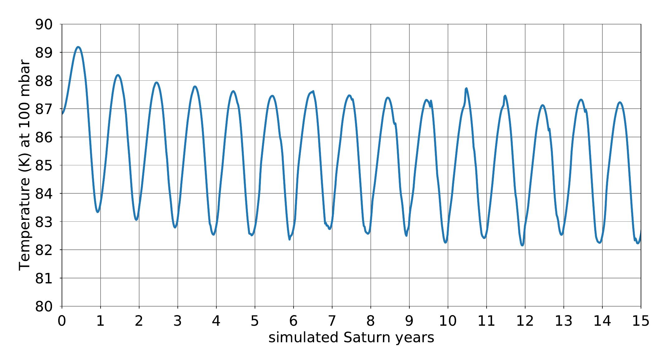
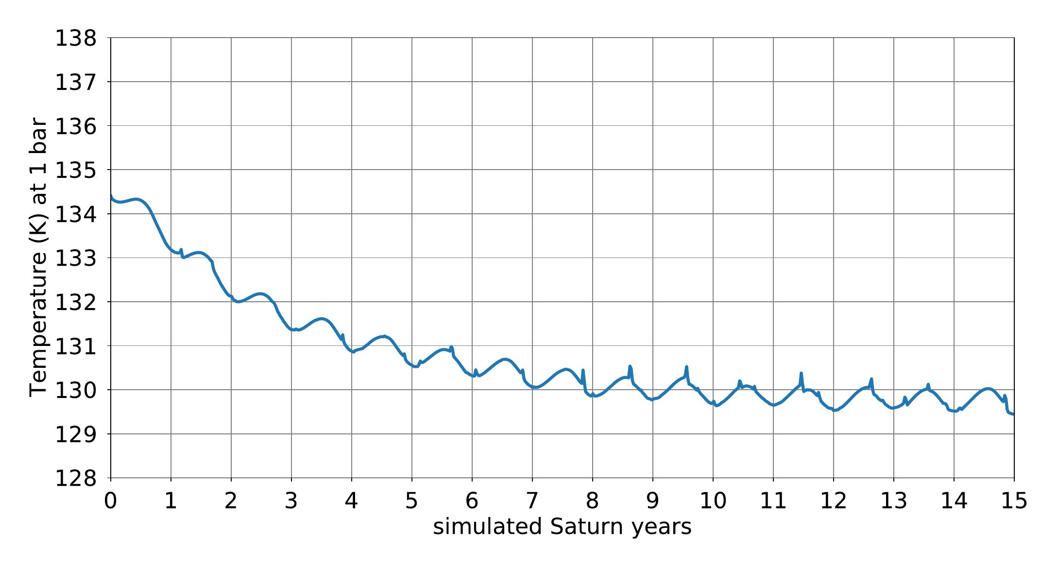
The analysis of angular momentum in appendix A.2 shows that the 15-year duration of simulation ensures dynamical spin-up and that the dynamical fields are in quasi-steady state. Full radiative spin-up must also be ensured, along with dynamical spin-up. In Figure 1 the evolution of the mean temperature in the northern hemisphere is shown: as is expected from differences in radiative timescales, the troposphere takes longer to reach steady-state seasonal cycle (about eight Saturn years) than the tropopause level does (about three Saturn years). This shows that satisfactory spin-up, both dynamical and radiative, is ensured starting from the ninth simulated year.
The comparison of our seasonal radiative-convective model with observations, both from instruments on board the Cassini spacecraft and ground-based telescopes, is discussed at length in Guerlet et al., (2014). Yet a sanity check is necessary, given that we now use this model interactively with a three-dimensional dynamical core.
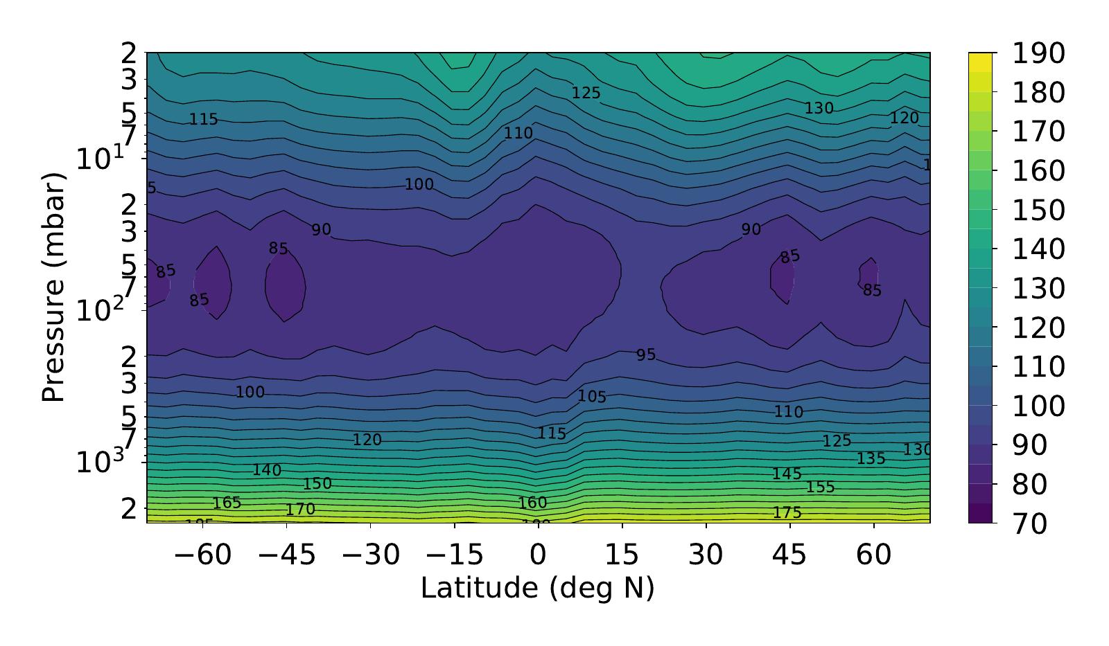
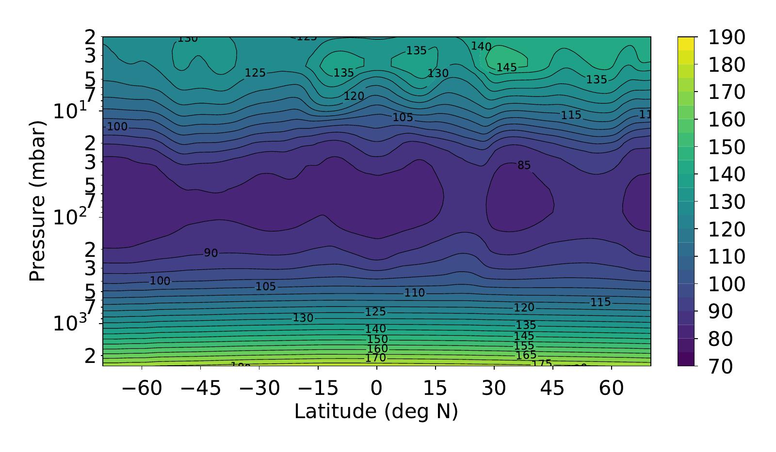
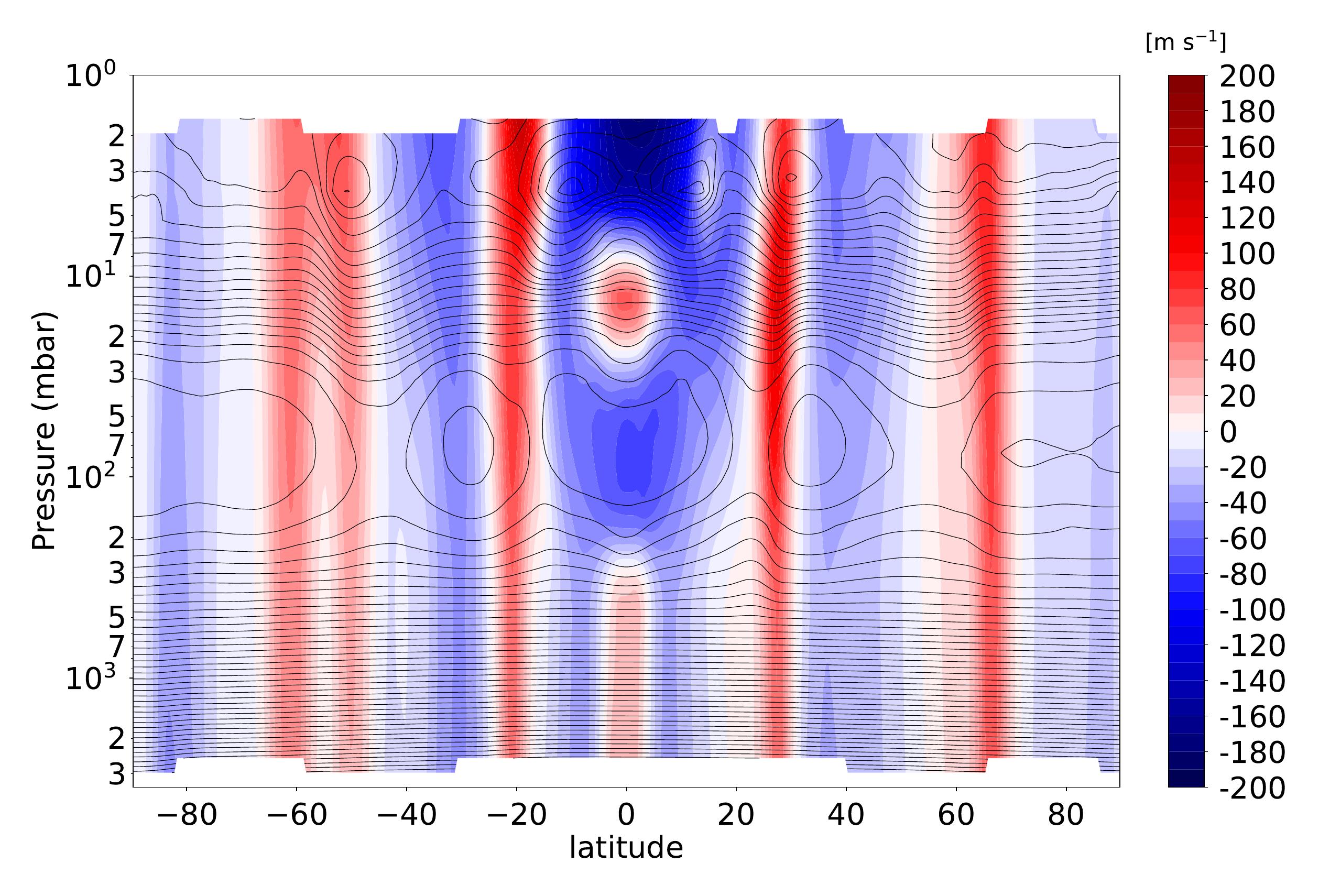
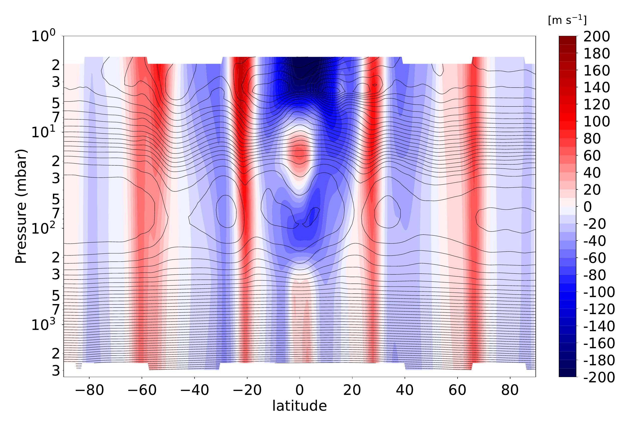
Figure 2 shows meridional-vertical sections of zonal-mean temperatures, both simulated by our Saturn DYNAMICO GCM and observed by the Cassini / Composite InfraRed Spectrometer (CIRS) instrument in 2015. The model successfully reproduces the vertical transition from troposphere to stratosphere, and the rather flat meridional gradients of temperature at this season (). In Figure 3 (top), the simulated meridional-vertical section of the Brunt-Väisälä frequency indicates that the radiative-convective transition, between the neutral profile () in the bulk of the troposphere and the stable profile () in the upper troposphere and lower stratosphere, occurs around mbar, which is in agreement with observations (Pérez-Hoyos and Sánchez-Lavega,, 2006; Fletcher et al.,, 2007).

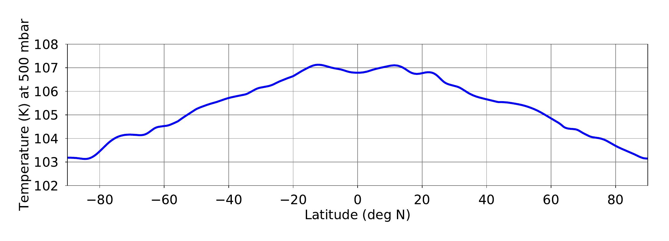
Nevertheless, while a K contrast between low latitudes and the pole is observed by Cassini at 500 mbar (Fletcher et al., 2010a, , Figure 3 bottom), the simulated pole-to-equator meridional gradient of temperature in our Saturn DYNAMICO GCM at the 500 mbar level is about K (Figure 3 bottom). This is half of the meridional gradient simulated by Liu and Schneider, (2010), but still at least twice the observed gradient. Most of the incident solar flux on Saturn is absorbed in the upper troposphere haze (Pérez-Hoyos and Sánchez-Lavega,, 2006; Fletcher et al.,, 2007), but our radiative model (Guerlet et al.,, 2014) shows that the solar flux is not zero at mbar and enough to cause a hemispheric meridional gradient of temperature.
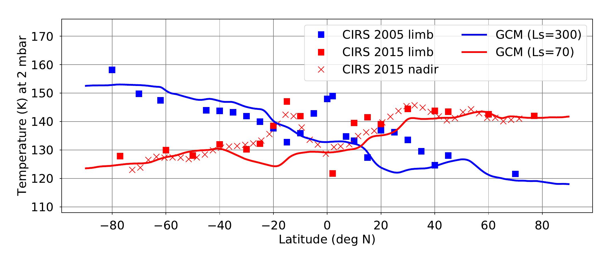
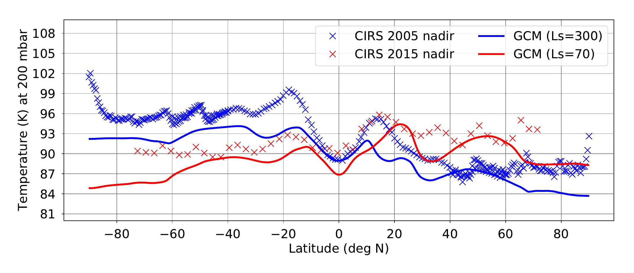
A more detailed comparison than Figure 2 is displayed in Figure 4, at two typical pressure levels where Cassini/CIRS is the most sensitive, close to the two solstices within which Cassini was operating. The meridional gradient of temperature, and the seasonal variability thereof, is correctly represented in our model. The fact that summer stratospheric temperatures are K too warm compared to CIRS observations was also noted with one-column radiative-convective modeling (Guerlet et al.,, 2014; Sylvestre et al.,, 2015) and is not a feature introduced by our dynamical simulations. Putative dynamical effects (e.g. Brewer-Dobson seasonal circulations) had been proposed to explain this discrepancy between radiative models and CIRS observations; however, the adopted setting for our Saturn DYNAMICO GCM simulations does not allow us to address this question that would require to raise the model top above the 1-mbar level.
The zonal jets produced by our dynamical model (discussed at length in what follows) are associated with distinctive temperature signatures, i.e. localized meridional gradients of temperature (see Figure 2 and 4), according to the thermal wind equilibrium which links to . These thermal signatures associated with jets are of similar amplitude between modeling and observations, although the localization (i.e. latitude) of those thermal signatures is not compliant between models and observations, echoing the discrepancies in latitude between the observed and modeled jet structures (see section 3.2).
3.2 Tropospheric and stratospheric jets
3.2.1 Mid-latitude jets
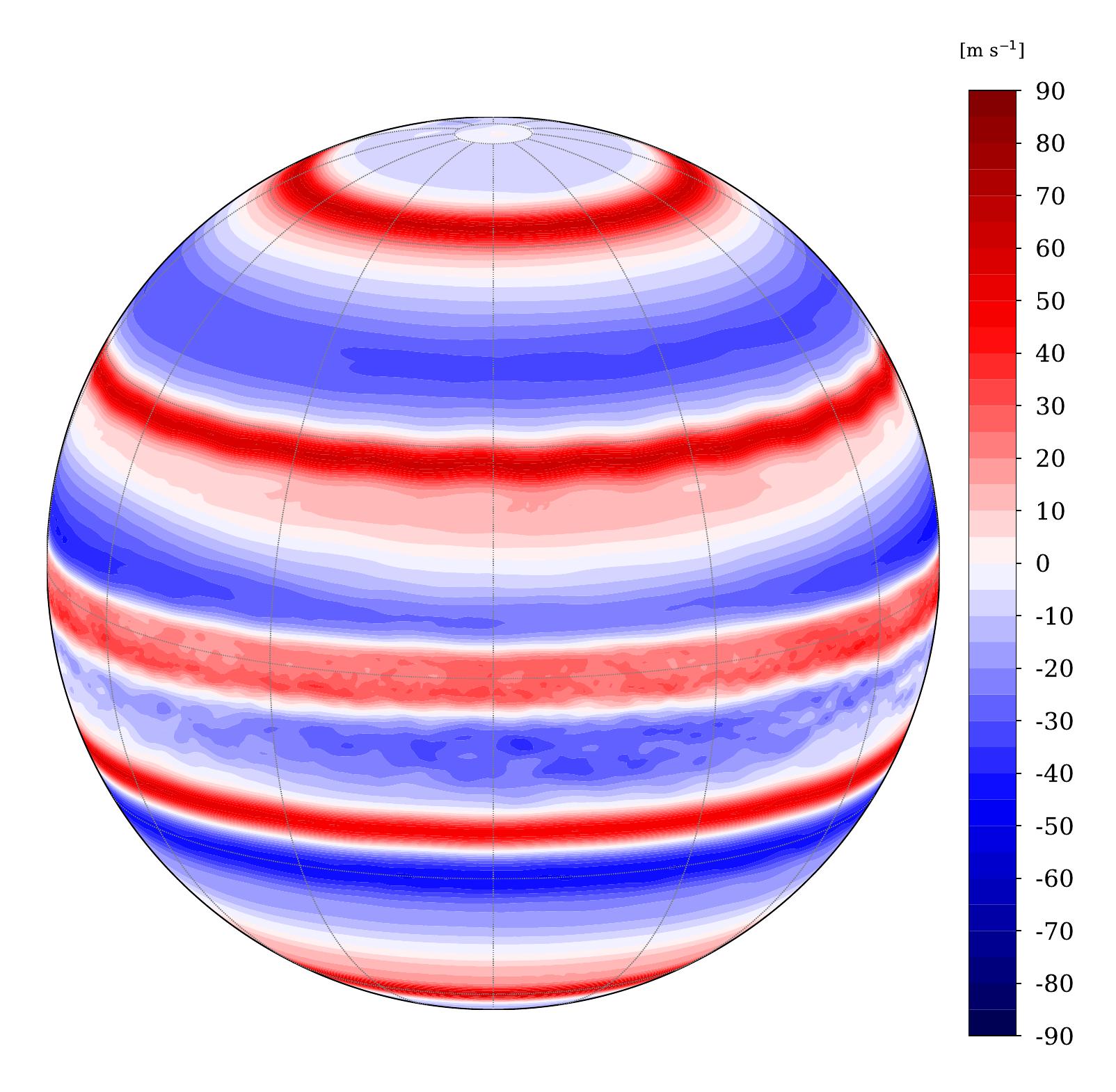
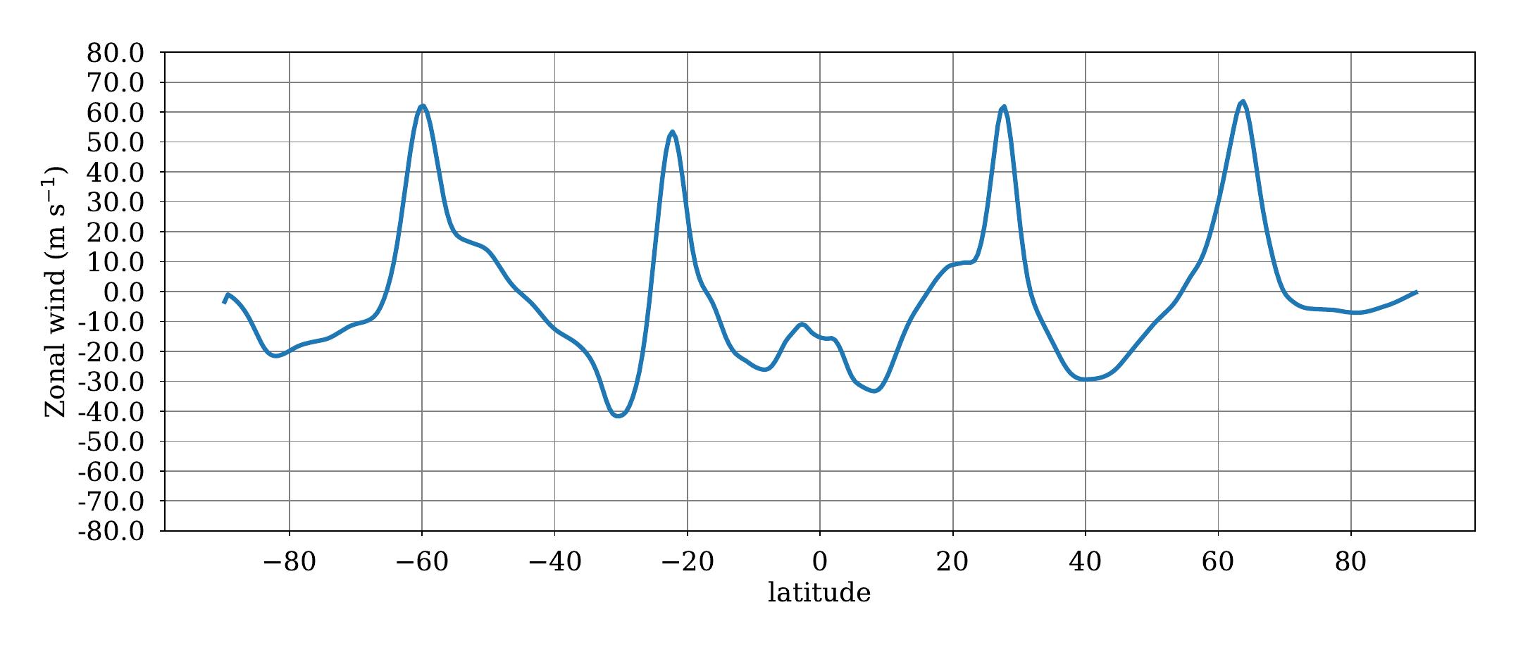
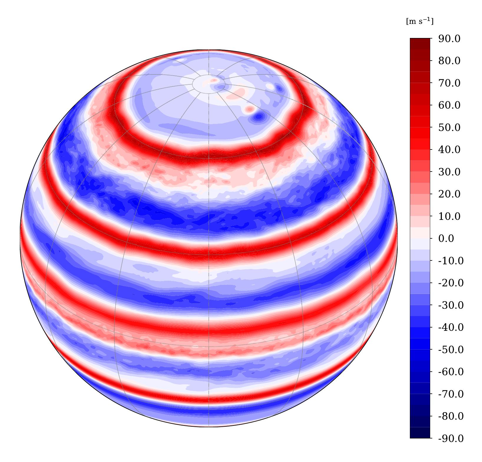
Figure 5 is a snapshot of the steady-state zonal flow of our Saturn DYNAMICO GCM simulation. Our model produces mid-latitude zonal jets, both eastward and westward (i.e. prograde and retrograde), which average intensities over a year reach about m s-1 for westward jets and m s-1 for eastward jets at the visible cloud deck ( bar). Thus the strength of mid-latitude zonal jets modeled in our Saturn DYNAMICO GCM are, to first order, consistent with the observed winds (Porco et al.,, 2005; García-Melendo et al.,, 2010) recast in the System IIIw rotating frame following Read et al., 2009b (see their Figure 2a). The quantitative match between our GCM and the observations is not perfect, for modeled mid-latitude jets are underestimated by about compared to observations. Although the number of mid-latitude prograde zonal jets produced in our Saturn DYNAMICO GCM is compliant with observations ( per hemisphere), the latitude of occurrence of the modeled zonal jets do not exactly match the observations, where the mid-latitude jets are more closely grouped. Our GCM predictions for mid-latitude zonal jets are broadly consistent with the previously-published body of work employing Saturn GCMs (e.g., Liu and Schneider,, 2010; Lian and Showman,, 2010).
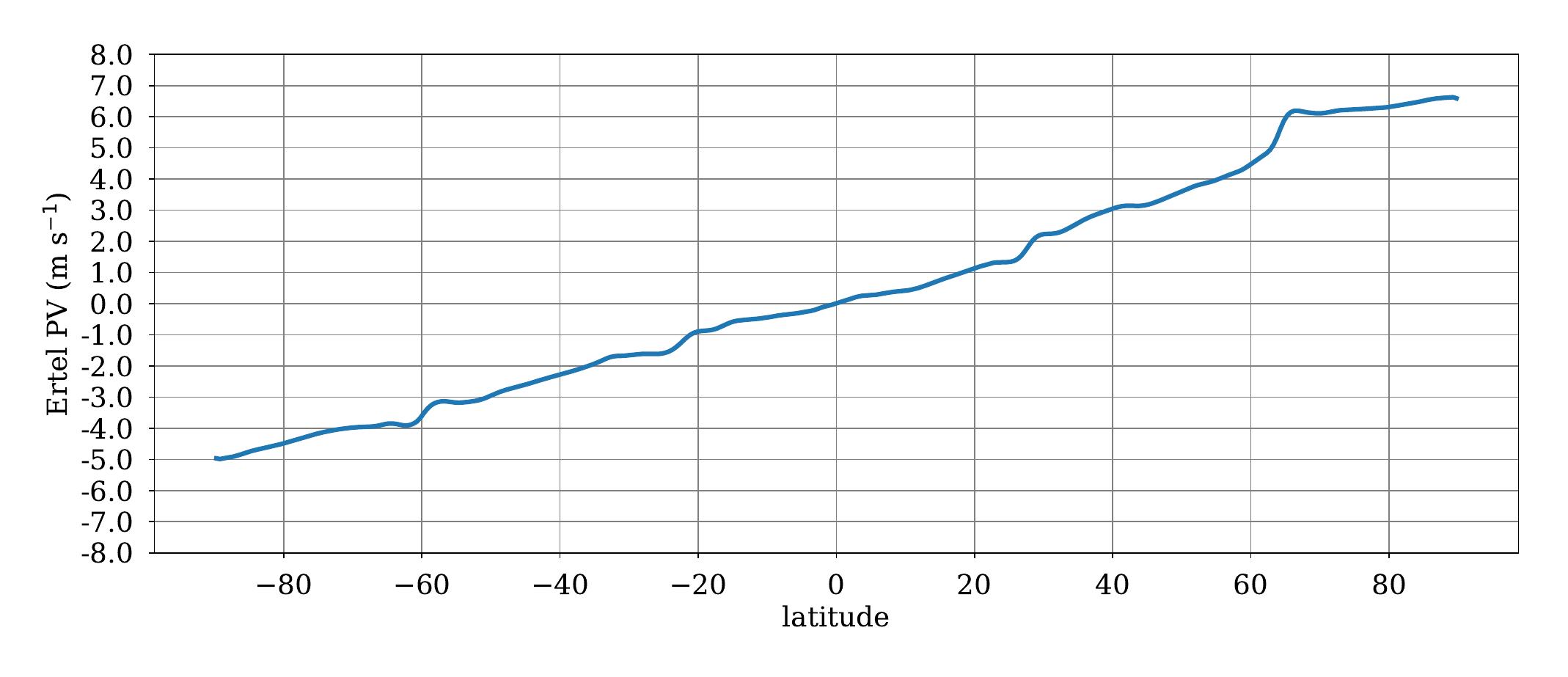
The Ertel potential vorticity (PV) calculated on isentropic surfaces – a conserved quantity (i.e. a flow “tracer”) for adiabatic motions (Vallis,, 2006) – is defined under hydrostatic approximation following Read et al., 2009a equation 3
| (1) |
where and are defined as in Table 1, with the subscript denoting evaluation across a surface of uniform potential temperature . The meridional profile of PV associated with the tropospheric jet structure simulated by our Saturn DYNAMICO GCM is shown in Figure 6. Characteristic PV “staircases” (i.e. sharp PV gradients) are found within the core of each mid-latitude eastward jet, surrounded by areas with “mixed PV” (i.e. uniform PV with latitude) on the flanks of the jets. The Ertel PV field obtained in Figure 6 with our model is similar to the one obtained through Cassini measurements by Read et al., 2009a . This result, reminiscent of those obtained with idealized models of rapidly-rotating flows (Dunkerton and Scott,, 2008; Dritschel and Scott,, 2011; Marcus and Shetty,, 2011), shows that the emergence and sharpening of mid-latitude eastward jets is associated with PV mixing. This homogeneization of PV on the flanks of the jets is associated with the breaking of Rossby waves emitted at the core of the jet (e.g., Dritschel and McIntyre,, 2008). This creates a convergence of eastward momentum towards the regions of wave emission, i.e. the core of the eastward jets (Vallis,, 2006; Schneider and Liu,, 2009; Showman and Polvani,, 2011), helping to maintain the jet structure against dissipation (O’Gorman and Schneider,, 2008).
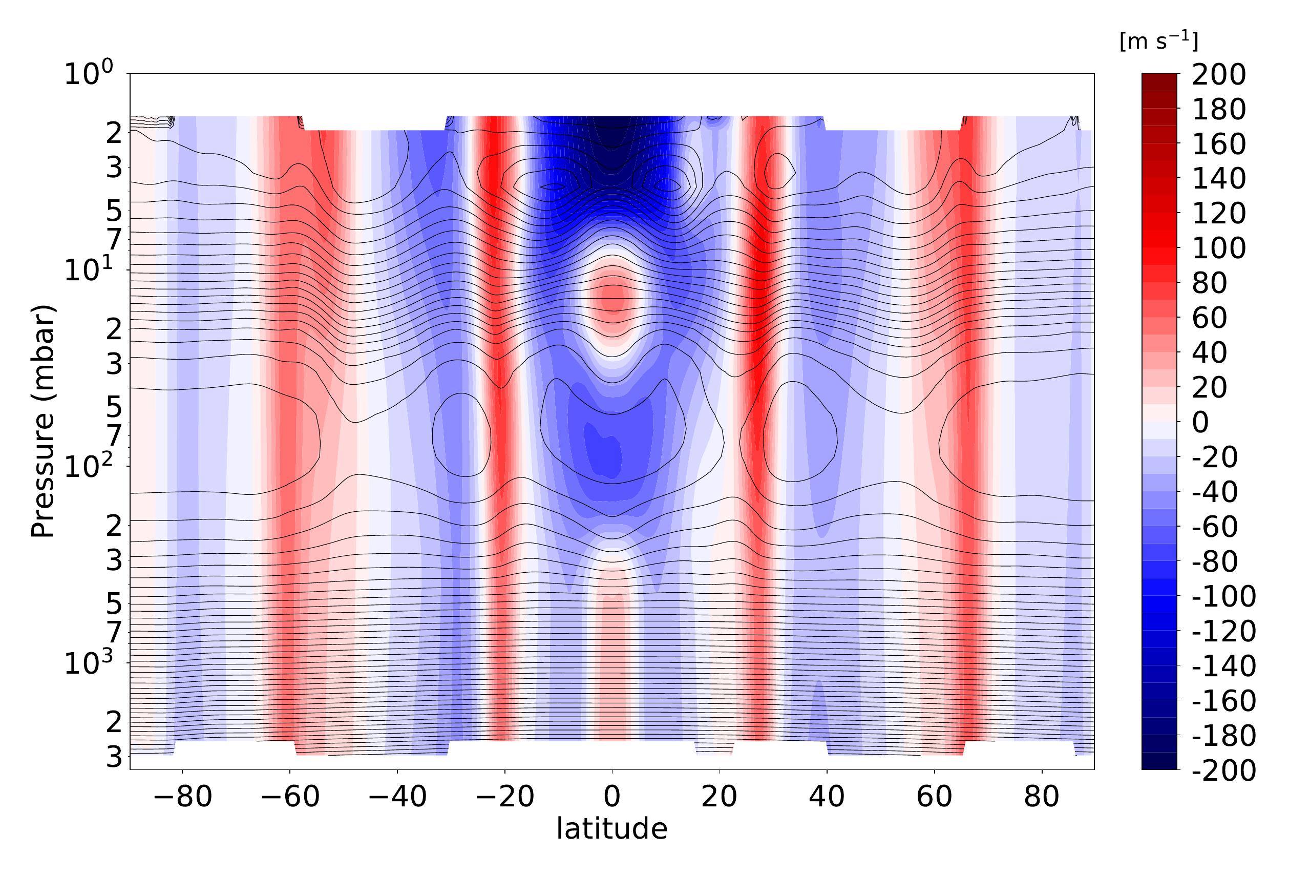
The vertical structure of the zonal-mean zonal jet system simulated by our Saturn DYNAMICO GCM is displayed in Figure 7. The mid-latitude eastward and westward jets exhibit a barotropic structure (i.e. weak vertical shear) in the deep troposphere, and a baroclinic structure (i.e. significant vertical shear) in the upper troposphere / stratosphere. The latter is in balance with the meridional temperature variations observed and modeled in the temperature structure in Figure 4. Interestingly, eastward mid-latitude jets simulated in our Saturn DYNAMICO GCM does not weaken from the cloud level around 1 bar to the upper troposphere, as is observed (García-Melendo et al.,, 2010; Del Genio and Barbara,, 2012); the jet intensity actually tends to slightly increase upwards from the troposphere to the stratosphere in our simulations. Using Cassini VIMS images, Studwell et al., (2018) found that the intensities of mid-latitude jets were generally increasing from the 2-bar level to the 300-500 hPa level, which tends to confirm our Saturn DYNAMICO GCM results at and below the cloud level.
Accounting for the preferential zonal wavenumber (hexagonal) mode in the circumpolar jet structure on Saturn is still an open question (Morales-Juberías et al.,, 2011, 2015), given the narrow parameter space which allows for this mode to predominate over other modes (Barbosa Aguiar et al.,, 2010; Rostami et al.,, 2017). The polar jet in our Saturn DYNAMICO GCM simulation (Figures 5 and 12) has a different morphology than the other mid-latitudes jets, exhibiting meandering with time, which cause it to undergo latitudinal deformation and temporal variability. However, the meandering of our simulated polar jet is intense and very variable with time, with neither a nor any mode predominance. This is clearly at odds with the observed stable slowly-moving hexagonal jet in Saturn’s northern polar regions (Sánchez-Lavega et al.,, 2014; Antuñano et al.,, 2015). The polar jet’s zonal wind speed, latitudinal position and width are, however, key factors to account for Saturn’s northern polar hexagon (Morales-Juberías et al.,, 2011). The polar jet simulated by our Saturn GCM is both too weak and too equatorward (as in Figure 5) to possibly lead to a predominance of the mode. Furthermore, the polar jet’s temporal evolution influenced by poleward migration causes it to break under intensified meandering by barotropic and baroclinic instability (see section 4). This obviously prevents any high-latitude jet to settle as a stable, wavenumber-6 hexagon-shaped, structure. Either the baroclinicity in the polar regions is not realistic enough in our Saturn DYNAMICO GCM (this influence of vertical shear is discussed in Morales-Juberías et al.,, 2015); and/or the central polar vortex is insufficiently resolved in our simulations, hence too weak to stabilize the hexagonal shape of the polar jet against meandering (the influence of the central polar vortex is discussed in Rostami et al.,, 2017).
3.2.2 Equatorial jets
A prograde equatorial jet is produced in the troposphere by our Saturn GCM simulation. It is, however, severely underestimated by one order of magnitude compared to the observed value by Cassini ( m s-1 in System IIIw, Read et al., 2009b, ; García-Melendo et al.,, 2010). The local super-rotation index associated with this equatorial jet writes (e.g., Read and Lebonnois,, 2018)
| (2) |
The equatorial zonal jet simulated by our GCM is only weakly super-rotating () in a very limited area across the equator (), while the observed superrotating index is an order of magnitude larger (Read and Lebonnois,, 2018, their table 1) and the observed equatorial jet extends towards latitudes .
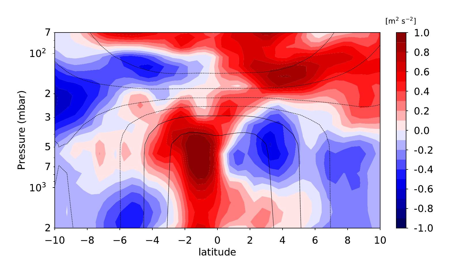
The prograde, eastward, equatorial jet in the Saturn DYNAMICO GCM arises from acceleration caused by convergence of eddy momentum towards the equator (see equation 13 in section 4). Figure 8 shows that, within the equatorial super-rotating jet, the eddy momentum transport is positive south of the equator and negative north of the equator, meaning that waves and eddies cause a convergence of eastward momentum at the equator. Yet this equatorial acceleration by waves and eddies is probably underestimated by our Saturn DYNAMICO GCM, given the resulting modeled jet being ten times less strong than the observed equatorial jet (García-Melendo et al.,, 2010). This is consistent with the latitudinal profile of Ertel PV shown in Figure 6, where PV mixing by Rossby waves in equatorial regions appears not sufficient to yield a truly PV-mixed area, as is the case for mid-latitude jets.
Based on the existing literature (e.g., Gierasch et al.,, 2000; Lian and Showman,, 2010), a possible source of this underestimate of Saturn’s equatorial superrotation could be the lack of a parameterization for moist convection in our model (see, e.g., the work on Jupiter by Zuchowski et al.,, 2009; Young et al., 2019b, ). Our GCM results are actually in contrast with the simulations by Liu and Schneider, (2010) which did not include an additional (moist) convective source, apart from the combination of internal heat flux and convective adjustment. The fact that the convective adjustment scheme in Liu and Schneider, (2010) has a non-zero relaxation time (cf. Schneider and Liu,, 2009, appendix B, section d), while ours is instantaneously adjusting, might be an element of explanation for this discrepancy. Using a non-zero relaxation time might emulate the convective overturning time of dry and moist convective structures, confirming the need to add, in our Saturn DYNAMICO GCM, a (dry and moist) convective parameterization more sophisticated than our simple convective adjustment scheme (e.g. thermal plume modeling like Hourdin et al.,, 2002; Rio and Hourdin,, 2008; Colaïtis et al.,, 2013) that will better represent the local dynamics underlying convective mixing and the impact thereof on the generation of waves and eddies.
While the strengths of mid-latitude jets increase with altitude in our Saturn DYNAMICO GCM simulations (see section 3.2.1), the intensity of the simulated equatorial jet decreases with altitude, which is also in line with the Cassini observations reported in Studwell et al., (2018). Although a quantitative comparison with observations is prevented by the severely underestimated equatorial wind speed in our GCM, the fact that the equatorial jet decays from the cloud level to the tropopause is also observed by Flasar et al., (2005), Li et al., (2008), and Sánchez-Lavega et al., (2016). Figure 8 indicates that this decay is caused in our Saturn DYNAMICO GCM by divergence of eastward eddy momentum at the tropopause, in contrast to the convergence of eastward eddy momentum causing the super-rotating jet in the troposphere. Interestingly, to interpret the Cassini VIMS observations of tracers, Fletcher et al., 2011a proposed that two stacked, reversed cells are present in Saturn’s troposphere, one resulting from “jet damping” in the upper troposphere and one resulting from “jet pumping” in the mid-troposphere (their section 6). This is compliant with Figure 8 showing in equatorial regions an area of eddy divergence / westward jet sitting on top of an area of eddy convergence / eastward jet.
Saturn’s equatorial stratosphere exhibits a downward propagation of (supposedly zonally-symmetric) alternating positive and negative temperature perturbations with respect to the radiative-equilibrium temperature field (Fouchet et al.,, 2008; Guerlet et al.,, 2011; Li et al.,, 2011; Fletcher et al.,, 2017; Guerlet et al.,, 2018). Those temperature signatures are thought to be associated with eastward and westward jets alternating along the vertical, similarly to the Earth’s Quasi-Biennal Oscillation (Baldwin et al.,, 2001). The typical period of this equatorial stratospheric oscillation is Earth years, half a Saturn year (Orton et al.,, 2008). Modeling could help to identify the mechanisms responsible for Saturn’s equatorial oscillation, putatively the interaction of planetary-scale and small-scale waves with the mean zonal flow as it is the case of the terrestrial Quasi-Biennal Oscillation (Baldwin et al.,, 2001).
In Figure 7, above the eastward equatorial tropospheric jet, we note the presence in our reference simulation of stacked, alternatively eastward and westward, stratospheric jets. An eastward jet is centered at pressure level mbar in the latitudinal range N, surrounded above and below by westward jets. This structure is reminiscent of the stacked jet signature derived through thermal wind balance from Cassini observations of equatorial oscillation of temperature (e.g., Guerlet et al.,, 2018). Yet, contrary to Cassini observations, no downward propagation of this jet signature is reproduced by our Saturn DYNAMICO GCM between northern summer and fall (Figure 9).
Section 3.3.1 features a discussion of the equatorial waves being most probably responsible for the stacked jet structure in the stratosphere, and possible explanations for the lack of vertical propagation of the structure. A key point, not related to the wave analysis, that shall be emphasized here is that the model top is too low (at 1 mbar), and the vertical resolution of the model in the stratosphere is too coarse, to correctly study the observed equatorial oscillations. For instance, the equatorial westward jet above 10 mbar is compliant with the thermal wind field derived by Fouchet et al., (2008), but our too-low model top prevents us from discussing the bulk of the observed oscillation above the 10-mbar pressure level.
3.3 Waves and vortices
3.3.1 Equatorial waves
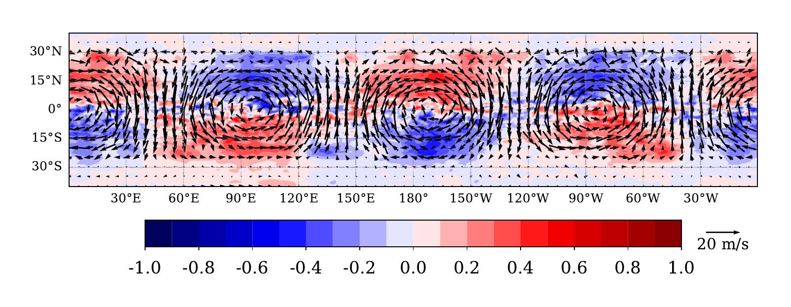
A close examination of the tropical structure of zonal wind in Figure 5 hints at planetary wave activity – notably a prominent wavenumber-2 signal. This is confirmed by Figure 10 in which the eddy (non-axisymmetric) components are shown in the equatorial region at the tropopause level. The prominent wavenumber-2 signal features zonal wind and temperature perturbations (about K) which are anti-symmetric about the equator, while meridional wind perturbations are symmetric about the equator. The pattern shown in Figure 10 is strongly reminiscent of an equatorial Yanai wave (also named mixed Rossby-gravity wave, Kiladis et al.,, 2009, their Figure 3), although an interpretation as an eastward inertio-gravity wave is also possible at this stage of the analysis.
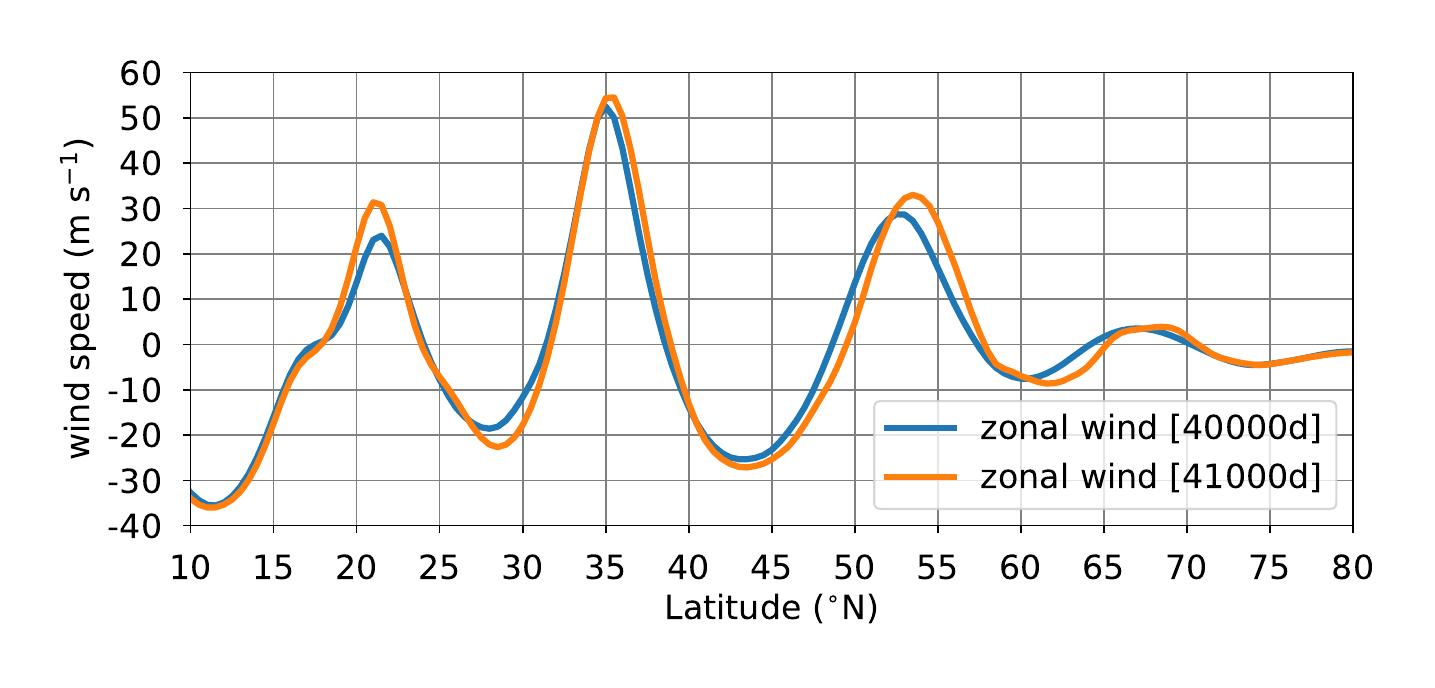
To further characterize the wavenumber-2 signal, and offer a more complete wave analysis (Figure 10 hints at other signals being present besides the prominent wavenumber-2 signal), we follow the method of Wheeler and Kiladis, (1999) commonly employed to study equatorial waves in the terrestrial tropical atmosphere (Kiladis et al.,, 2009; Maury and Lott,, 2014). We perform a two-dimensional Fourier transform, from the longitude / time space to the zonal wavenumber / frequency space, of the symmetric () and antisymmetric () components of the temperature field about the equator
| (3) |
(similar computations are also performed for zonal wind and meridional wind ). Our code uses the Fast Fourier Transform package included in the scipy Python library. We validated independently our spectral analysis code on well-defined (semi-)diurnal tides and Kelvin waves simulated in the Martian atmosphere (Wilson and Hamilton,, 1996; Lewis and Barker,, 2005; Guzewich et al.,, 2016).
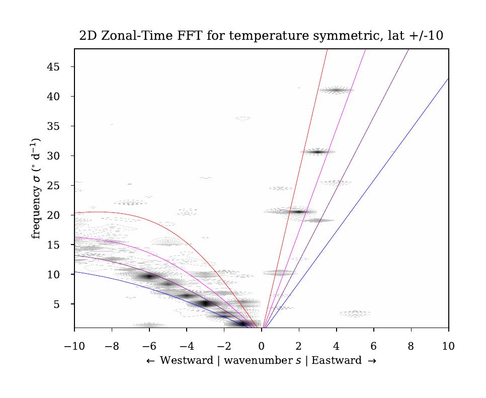
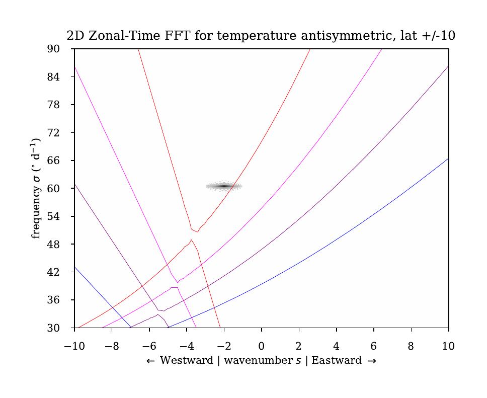
We perform the Fourier analysis on a specific 1000-day-long Saturn DYNAMICO GCM run with frequent (daily) output, restarted from the GCM state after thousands simulated Saturn days (about 11 simulated Saturn years). The spectral mapping in the space enables to evidence Rossby and Kelvin waves in the symmetric component and Yanai waves in the antisymmetric component (the former waves can also be detected in and the latter waves in and , see Wheeler and Kiladis,, 1999; Kiladis et al.,, 2009). Results for the temperature field simulated at the tropopause are shown in Figure 11, along with the dispersion relation for equatorial waves (Maury and Lott,, 2014)
| (4) |
where is the meridional mode number and defines the considered wave (Rossby: Yanai: , Kelvin: ), is named the Lamb parameter, and is an equivalent depth associated with the vertical wavenumber
| (5) |
Dominant modes in the symmetric and antisymmetric components of the temperature and wind fields are detailed in Table 2.
| Dominant modes in | |||
| /d) | period (d) | log(SP) | |
| +2 | 22.0 | 16.3 | 7.9 |
| +3 | 32.1 | 11.2 | 7.6 |
| -3 | 3.5 | 102.0 | 7.5 |
| -6 | 8.2 | 43.8 | 7.4 |
| -4 | 5.0 | 72.4 | 7.3 |
| -2 | 1.4 | 262.7 | 7.3 |
| -5 | 6.8 | 53.2 | 7.2 |
| +4 | 42.5 | 8.5 | 7.2 |
| Dominant modes in | |||
| /d) | period (d) | log(SP) | |
| -6 | 8.2 | 43.8 | 9.8 |
| -2 | 3.5 | 102.0 | 9.7 |
| -3 | 3.2 | 113.6 | 9.6 |
| -4 | 4.3 | 84.7 | 9.6 |
| -5 | 5.3 | 67.5 | 9.4 |
| -7 | 8.9 | 40.3 | 9.4 |
| +2 | 22.0 | 16.3 | 9.3 |
| Dominant modes in , , | |||
| /d) | period (d) | log(SP) | |
| -2 | 59.0 | 6.1 | 10.1 |
The spectral analysis shows that (consistently in the three analyzed fields) the prominent wavenumber-2 signal is a westward-propagating Yanai wave with a period days (frequency longitude per day). Our analysis also evidences, both in the temperature and zonal wind fields, westward-propagating Rossby waves with wavenumbers to , exhibiting long periods of hundreds Saturn days and frequencies of a couple degrees longitude per day (the wavenumber- cannot be evidenced unambiguously since its intrinsic phase speed is too close to zero). The longer-period Rossby waves are modulating the temperature variability caused by the wavenumber-2 Yanai wave with a shorter 6-day period. The temperature field also features eastward-propagating Kelvin waves with wavenumbers , periods Saturn days, and frequencies a couple tens of degrees longitude per day; the Kelvin wave signal is much fainter in the zonal wind component. This Kelvin wave signal is absent from the temperature field lower in the troposphere, at the cloud level.
Elaborating from Voyager observations, Achterberg and Flasar, (1996) detected a Rossby wavenumber-2 signal in the tropics and mid-latitudes of Saturn’s tropopause (130 mbar), confined by vertical variations of static stability. A similar signal is present in our our Saturn GCM DYNAMICO simulations: 1 degree longitude per day corresponds to m s-1, hence the simulated Rossby wavenumber-2 signal has a phase speed of m s-1, which is compatible with the phase speed of the order m s-1 discussed by Achterberg and Flasar, (1996). Our Saturn DYNAMICO GCM results indicate that other tropical Rossby modes (wavenumbers 3, 4, 5, …) are likely to be significant within Saturn’s tropics. This is compliant with the recent analysis by Guerlet et al., (2018), based on Cassini CIRS observations, which shows a complex structure at a pressure level of 150 mbar; interestingly, what appears as a wavenumber-3 Rossby mode dominate in the upper stratosphere (0.5 to 5 mbar), possibly indicating conditions for breaking at this level or below for the other modes. Unless the wavenumber-2 signal found by Achterberg and Flasar, (1996) is actually eastward-propagating at phase speeds about m s-1 (the fast planetary modes were discarded by this study in favour of slower, more plausible, Rossby modes), the prominent wavenumber-2 westward-propagating Yanai wave in our Saturn DYNAMICO GCM simulation remains to be evidenced in observations. A westward-propagating wavenumber-9 Yanai wave mode has been, however, detected by Cassini CIRS in the upper stratosphere (1 mbar) by Li et al., (2008), but their observed temperature signature being symmetric about the equator (with a maximum at the equator) would be more compliant with a westward inertia-gravity wave (Guerlet et al.,, 2018).
The presence of equatorial vertically-propagating eastward Kelvin waves and westward Rossby and Yanai waves in our Saturn DYNAMICO GCM simulations at the 130-mbar level means that both eastward and westward momentum is transferred in the stratosphere where vertically-stacked westward/eastward jets are found (Figure 7 and section 3.2.2). This “stacked jets” equatorial signature is similar to the jet structure putatively associated with the equatorial oscillation of temperature (Fouchet et al.,, 2008; Guerlet et al.,, 2011). Nevertheless, our model does not reproduce the downward propagation of the observed equatorial oscillation in Saturn’s stratosphere (Guerlet et al.,, 2018), also obtained by idealized simulations (Showman et al., 2018b, ). Furthermore, the modeled temperature contrasts between the equator and latitudes associated with the stacked jets ( K, figure not shown) are much lower than the contrasts obtained by Cassini thermal infrared measurements ( K, Fouchet et al.,, 2008; Guerlet et al.,, 2018). Those discrepancies with observations are probably related to a weak transfer of momentum to the mean flow by the resolved waves in our model:
-
while our spectral analysis reveals a Kelvin-wave signal at the tropopause, moist convection in the deep troposphere of Saturn, not accounted for in the current version of our model, could cause convectively-coupled Kelvin Waves, which are an important component to explain the Quasi-Biennal Oscillation on Earth (Kiladis et al.,, 2009);
-
mesoscale (inertia-)gravity waves are not resolved by our model and are known to contribute to the momentum flux responsible for equatorial oscillations on Earth (Lindzen and Holton,, 1968; Lott and Guez,, 2013; Maury and Lott,, 2014) and this possibility has also been explored in Jupiter’s stratosphere (Cosentino et al.,, 2017);
-
the absence of a strong equatorial super-rotating jet in our simulations means that the vertical propagation (and possible filtering) of equatorial waves towards the stratosphere is different between our simulations and the actual Saturn’s atmosphere.
According to terrestrial modeling studies (e.g. Takahashi,, 1996; Nissen et al.,, 2000; Watanabe et al.,, 2008; Lott et al.,, 2014), our modeling setting is ultimately lacking two key elements to reproduce Saturn’s equatorial oscillation: the model top must be raised to cover the stratospheric levels ( mbar) where the stratospheric oscillation is observed, and the vertical resolution must be refined in the stratosphere. Those improvements, related to Challenge , are deferred to a dedicated future study of Saturn’s stratospheric circulations using our Saturn DYNAMICO GCM (Bardet D. et al., Part IV in preparation).
3.3.2 Extratropical eddies
Our reference simulation with the Saturn DYNAMICO GCM exhibits a variety of extratropical eddies, as is evidenced in Figure 12.
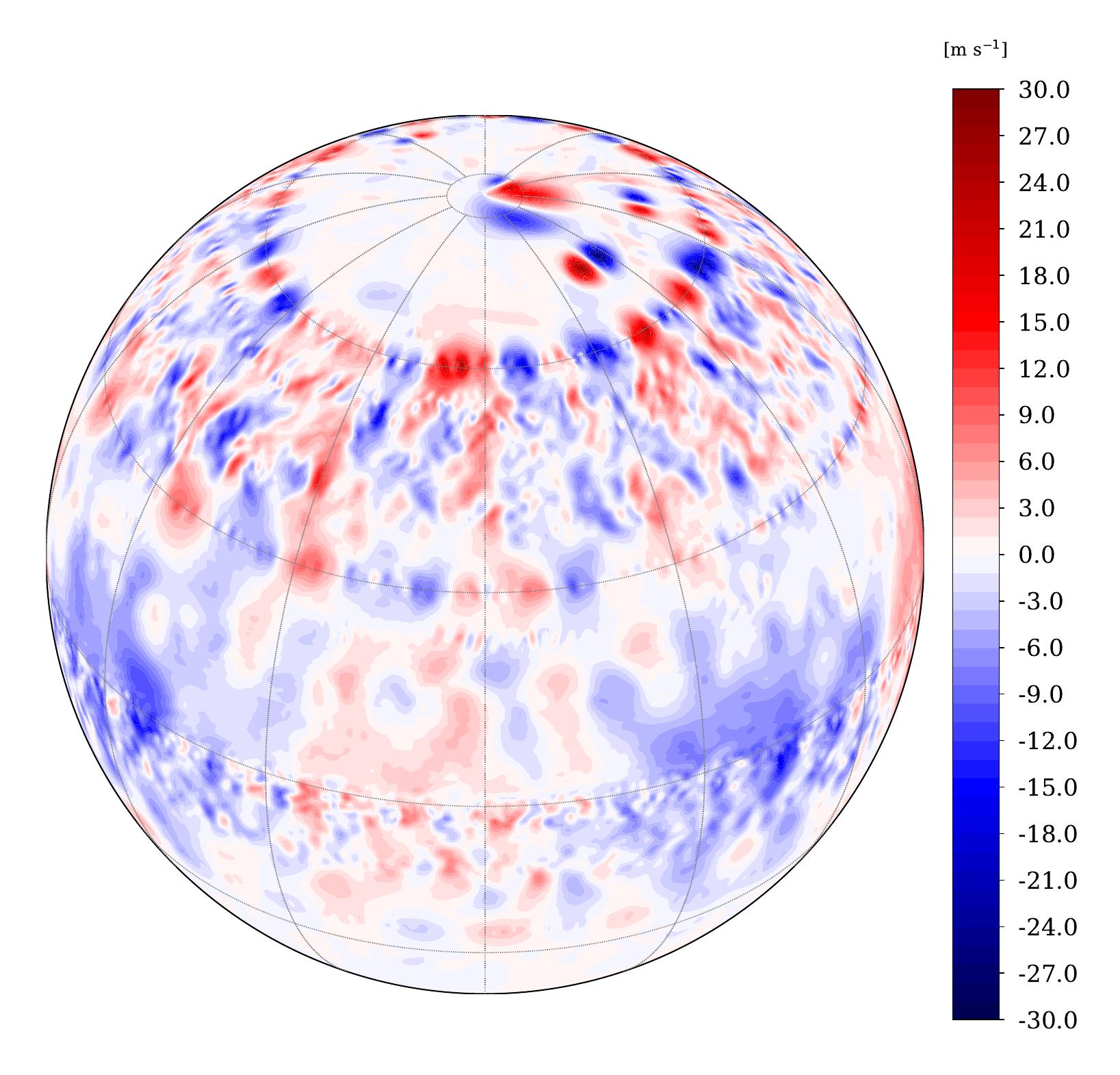
The simulated tropospheric fields in Figure 12 indicate that the mid-latitude eastward jets at latitude N and N are prone to meandering caused by high-wavenumber waves. Those waves are found at the center of the eastward jets, featuring a strong inversion of the meridional gradient of potential vorticity (Rayleigh-Kuo necessary condition for barotropic instability, see section 4.4). A spectral analysis on a 2000-day sample of the temperature and wind fields, performed similarly to the analysis in section 3.3.1 (except for a Doppler-shift correction considering the ambient eastward zonal jet m s-1) indicates that the 30∘N perturbations correspond to a westward-propagating wavenumber-19 Rossby wave with a period of days (frequency longitude per day, i.e. about 23 m s-1). The characteristics of this wave (wavenumber, phase speed, and occurrence at the center of a mid-latitude eastward jet) are very similar to the idealized modeling results obtained by Sayanagi et al., (2010) to explain the “Ribbon wave”, a Rossby wave propagating in the extratropical latitudes of Saturn as a result of barotropic and baroclinic instability (Godfrey and Moore,, 1986; Sanchez-Lavega,, 2002; Gunnarson et al.,, 2018). Furthermore, the meandering phase speed and wavenumber reproduced by our Saturn DYNAMICO GCM in the 30∘N eastward jet are compliant with the slow ribbon waves identified by Gunnarson et al., (2018) with Cassini imaging (their Figure 3d).
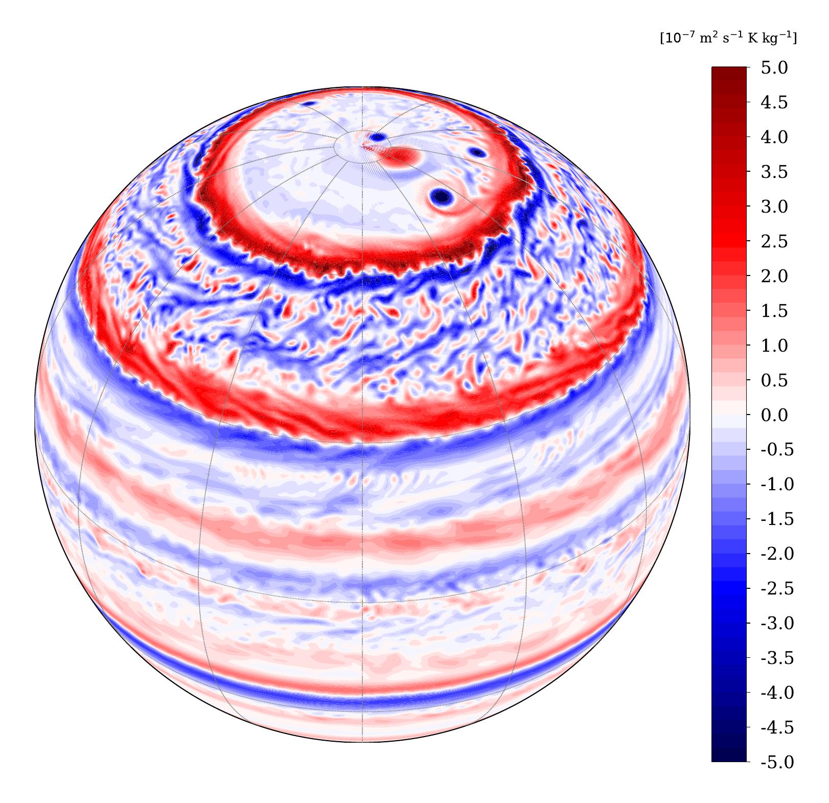
It is worthy of notice that our Saturn DYNAMICO GCM simulations exhibit a chain of about ten cyclonic vortices with an horizontal extent of a couple thousand kilometers (the successive red spots of positive vorticity in Figure 12 bottom) in the equatorward (southern) edge of the N eastward jet. This signature shares the characteristics of the “String of Pearls” observed by Cassini through infrared mapping (Sayanagi et al.,, 2014). Nevertheless, the simulated vortices are more short-lived (typically a ten-day duration) than the observed cyclonic vortices, so the analogy between the modeled structures and the “String of Pearls” is not complete.
The most distinctive and large-scale vortices are found in polar regions in our Saturn DYNAMICO GCM simulations. Figure 12 demonstrates a clear and sharp transition between the mid-latitudes where the vorticity field is dominated by eddies, and the polar regions where the vorticity field is dominated by large-scale vortices. This is somewhat compliant with the picture drawn by observations, where no vortex activity was observed in mid-latitudes before the appearance of the 2010 giant storm (Trammell et al.,, 2016). Both anticyclones and cyclones are produced in our model: the excerpt shown in Figure 12 comprises four anticyclones and one larger cyclone. Those simulated large-scale vortices exhibit a strong temporal variability, with merging phenomenon combined with beta-drift effect (poleward for anti-cyclones, see Sayanagi et al.,, 2013), which causes their typical duration to be no more than several hundreds Saturn days. The picture drawn by Figure 12 is typical of most of our Saturn DYNAMICO GCM simulation: anticyclones appear favored against cyclones, which is in agreement with the putative longer stability of anticyclones compared to cyclones, but at odds with the statistics derived from Cassini imagery over seven Earth years by Trammell et al., (2016). A more in-depth analysis of the large-scale vortices is out of the scope of this paper; furthermore, accounting for moist convection and the associated release of latent heat appears to be a crucial addition to carry out this analysis (O’Neill et al.,, 2015).
The last class of eddies are the remainder of non-axisymmetric disturbances that are neither waves nor vortices. Such “non-organized” eddies can be seen in Figure 12 between latitudes N and N. Their activity can strongly vary with time: Figure 12 shows a case with a “burst” of eddy activity at those latitudes, while the eddy activity can be close to none at other times in the simulation (Figure 5). The presence of intermittent bursts of eddy activity is reminiscent of the results of Panetta, (1993) and is further discussed in section 4.1.
4 Evolution of the tropospheric jet structure
4.1 Jets and eddies in the 15-year simulation
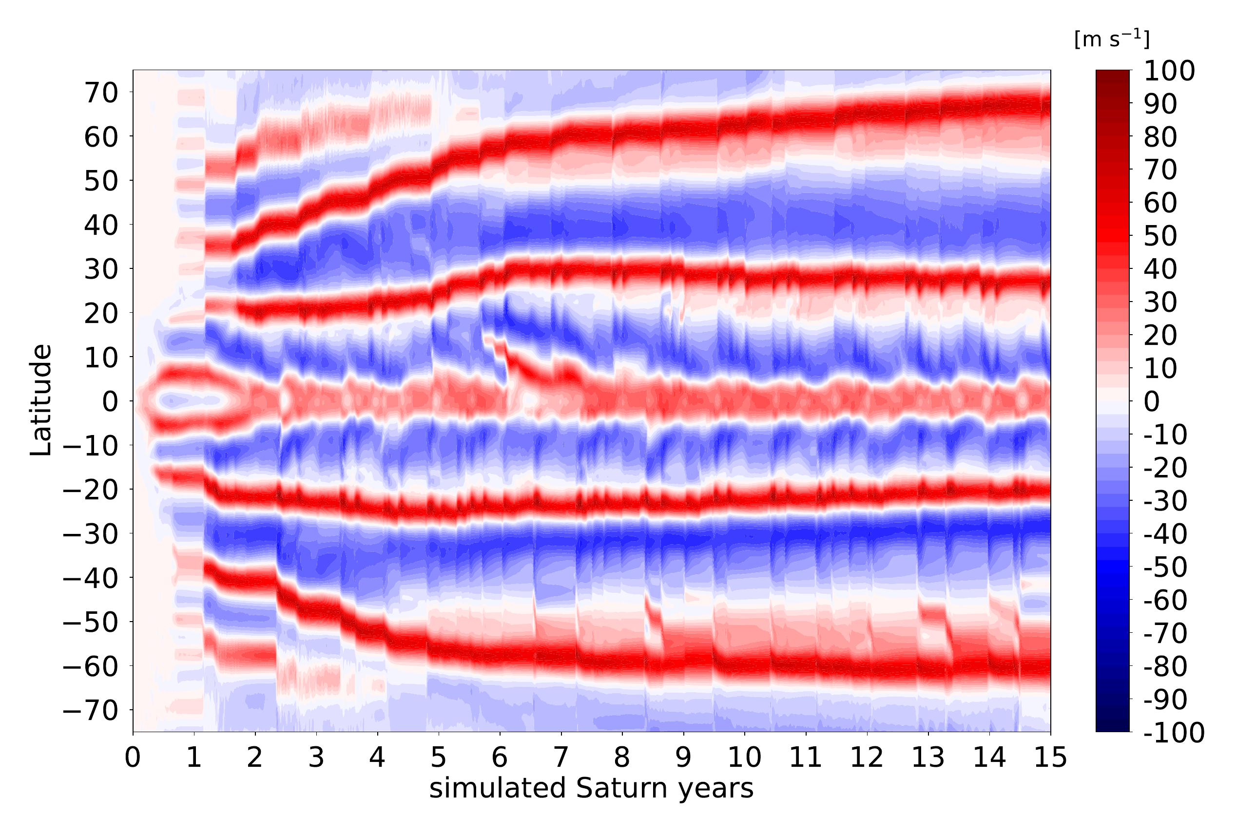
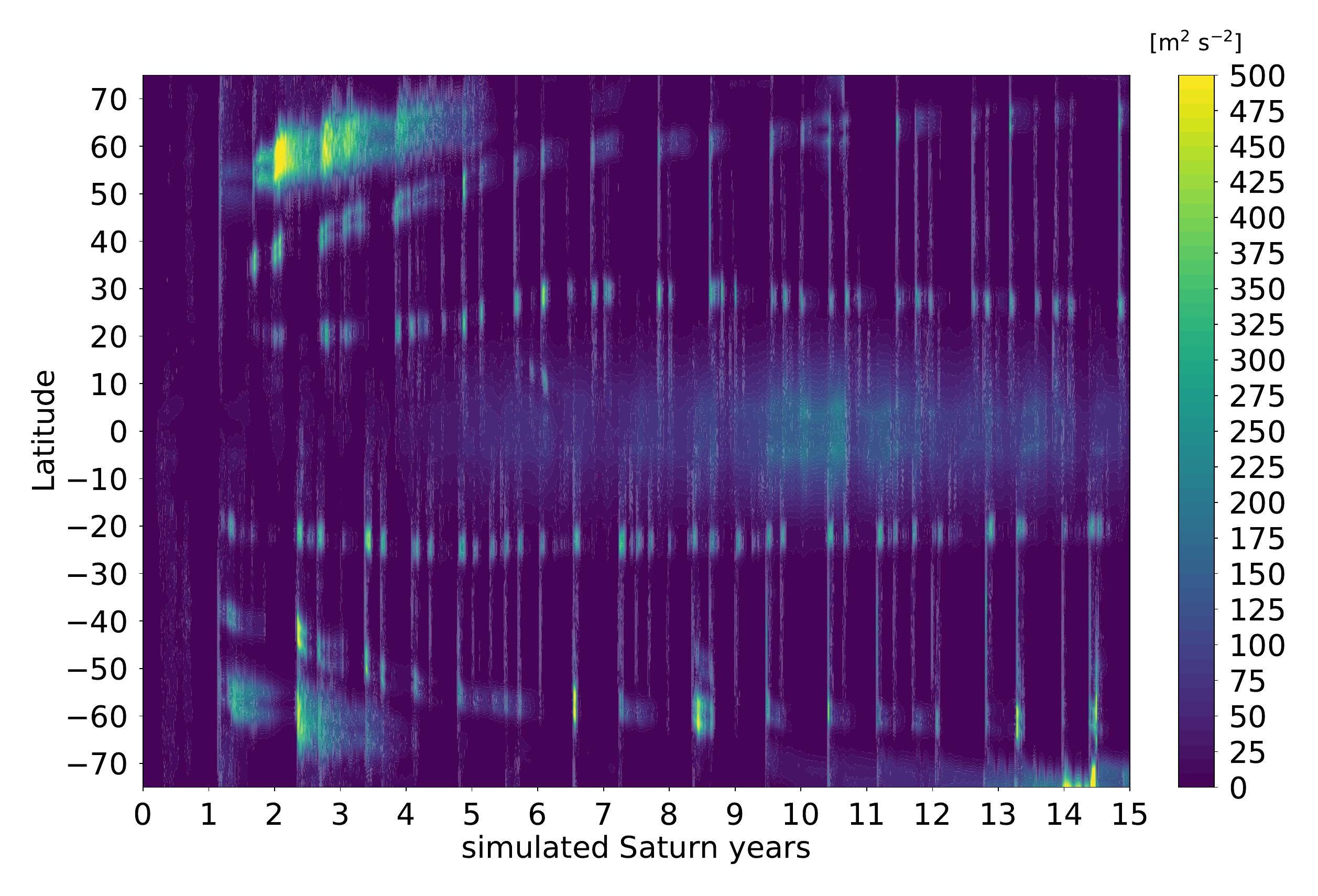
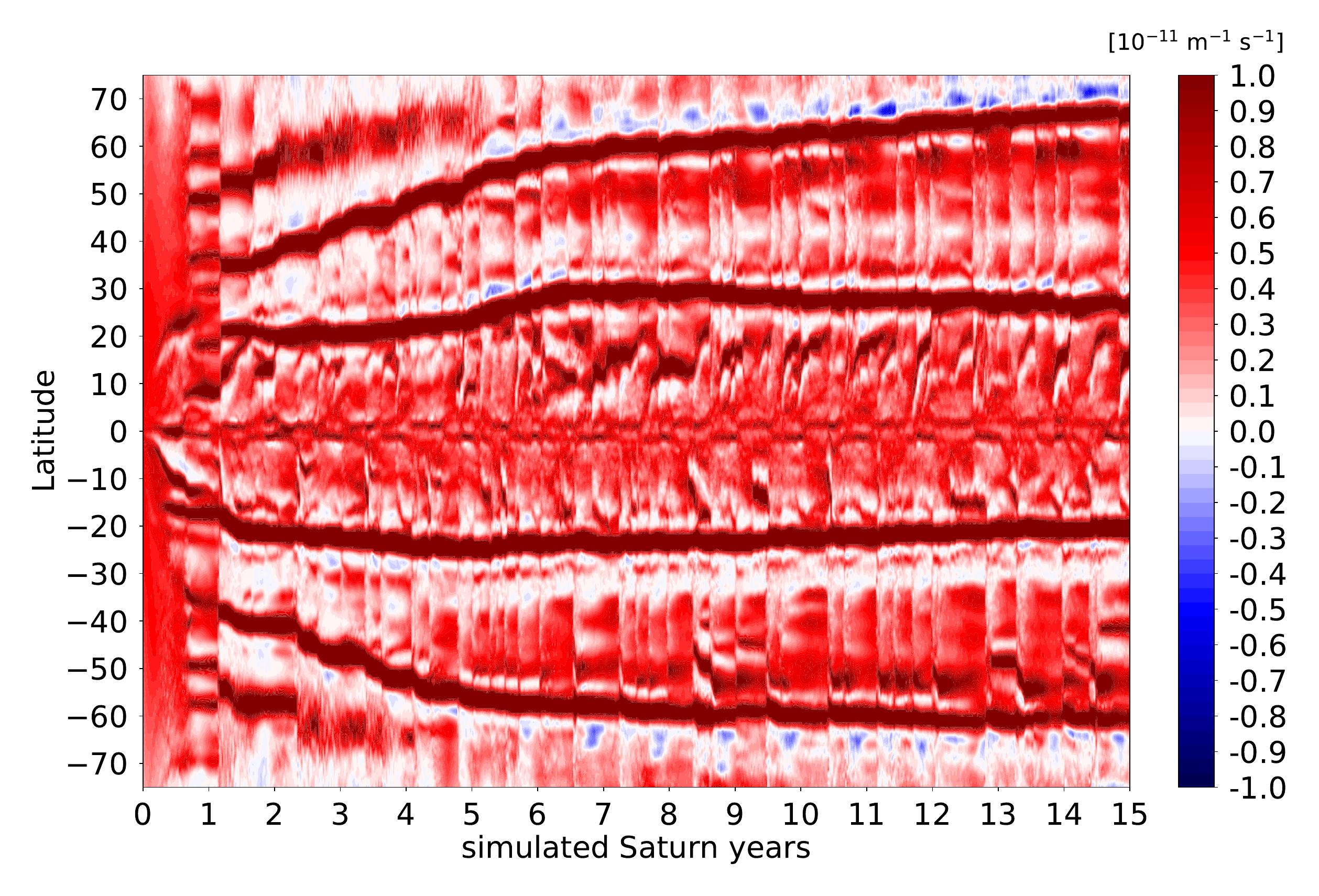
The evolution of tropospheric jets with time in the 15-year duration of our reference Saturn DYNAMICO simulation is summarized in Figure 13. It takes about about 6-7 simulated Saturn years for the jet system to reach what most closely resembles a steady-state equilibrium; a similar conclusion was drawn from the analysis of the temporal evolution of AAM (Figure 22 in section A.2). The zonal mean of the Eddy Kinetic Energy (EKE)
| (6) |
is also shown in Figure 13 to diagnose eddy activity.
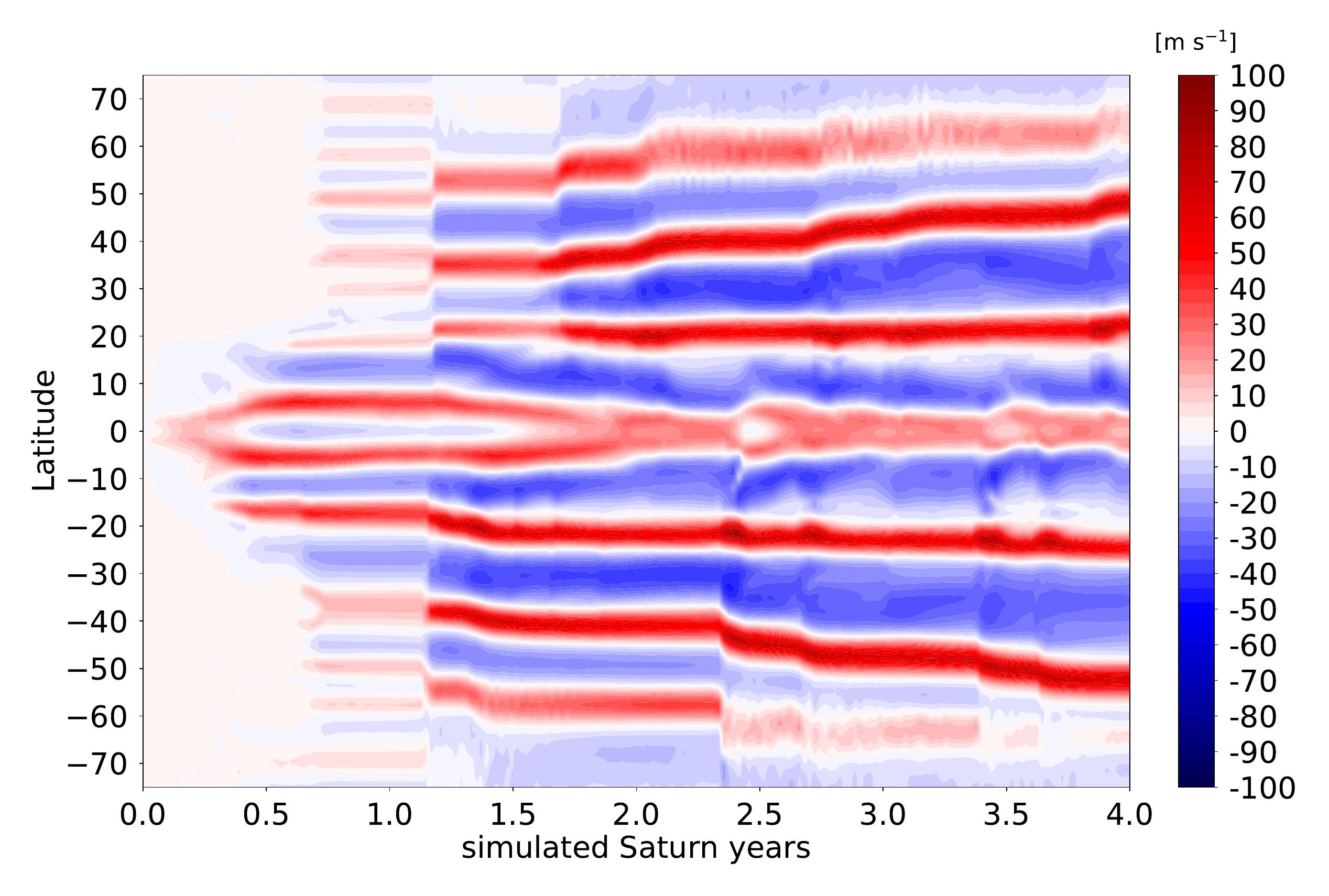
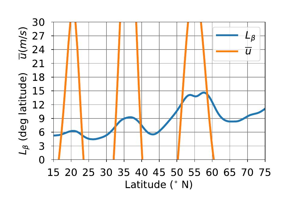
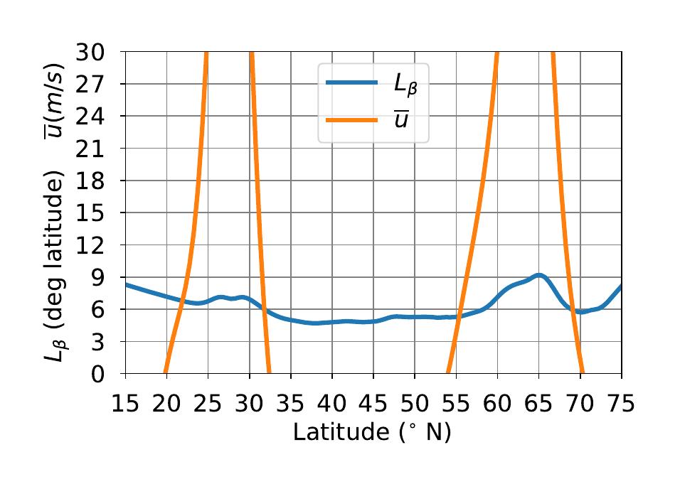
The first years of our Saturn DYNAMICO GCM simulations follow the evolution of zonal jets typically obtained with nonlinear analytical models prone to barotropic and baroclinic instability. The evolution of our Saturn DYNAMICO GCM displayed in the top panel of Figure 14 is similar to the evolution described, e.g., in Figure 10 of Kaspi and Flierl, (2007). The first simulated half-year exhibits no particular zonal organization (except at the equator). In the second half of the first simulated year, the growth of the fastest unstable mode leads to the emergence of numerous weak zonal jets, which subsequently reorganize, as additional growing eddy modes are present, to lead to a system with less, and wider, jets. The abrupt transition around 1.15 simulated years in Figure 13 is associated with significant eddy activity. The merging of numerous weak jets into a final jet structure with lesser and stronger jets is typical of the inverse energy cascade by geostrophic turbulence which shapes the jet structure (Cabanes et al.,, 2017). Another typical feature of the inverse energy cascade shown in Figure 15 is the overall correlation between the Rhines scale (Rhines,, 1975)
| (7) |
and the eastward jets’ width/spacing (Chemke and Kaspi, 2015b, ), with a tendency for broader jets and increased spacing between jets towards higher latitudes (Kidston and Vallis,, 2010). A full exploration of the dynamical regimes (e.g., zonostrophy) and the inverse energy cascade in our Saturn DYNAMICO GCM requires detailed spectral analysis of the flow energetics (Sukoriansky et al.,, 2002; Galperin et al.,, 2014; Young and Read,, 2017) that will be developed in a follow-up paper (Cabanes S. et al., Part III submitted).
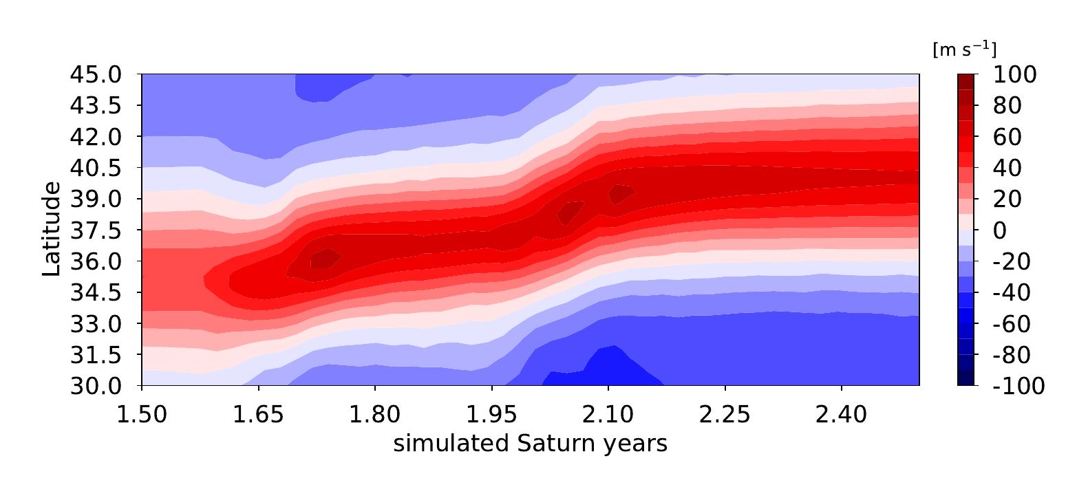
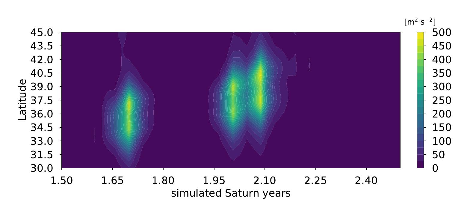
The most prominent feature of Figure 13 between the simulated years 1 and 6 is the poleward migration of mid-latitude jets. This echoes the idealized simulations detailed in Chemke and Kaspi, 2015a (see also jovian simulations by Williams,, 2003). The migration is gradual, but the jet migration is much stronger in short-lived episodes characterized by a burst of eddy activity, which implies momentum transfer to the jet altering its meridional structure. A detailed analysis of a typical poleward migration episode in Figure 13 is proposed in section 4.3. The tropical jets undergo a much weaker migration than the mid-latitude jets. Most of the migration events are poleward, but there is at least one clear equatorward migration event of a jet appearing at latitude N in the beginning of year 7. This equatorward migration contributes to accelerate the equatorial jet. This was also noticed by Young et al., 2019a in their Jupiter GCM, although their simulations exhibit a global tendency for equatorward jet migration, contrary to the global tendency for poleward jet migration found in our GCM simulations and in Chemke and Kaspi, 2015a .
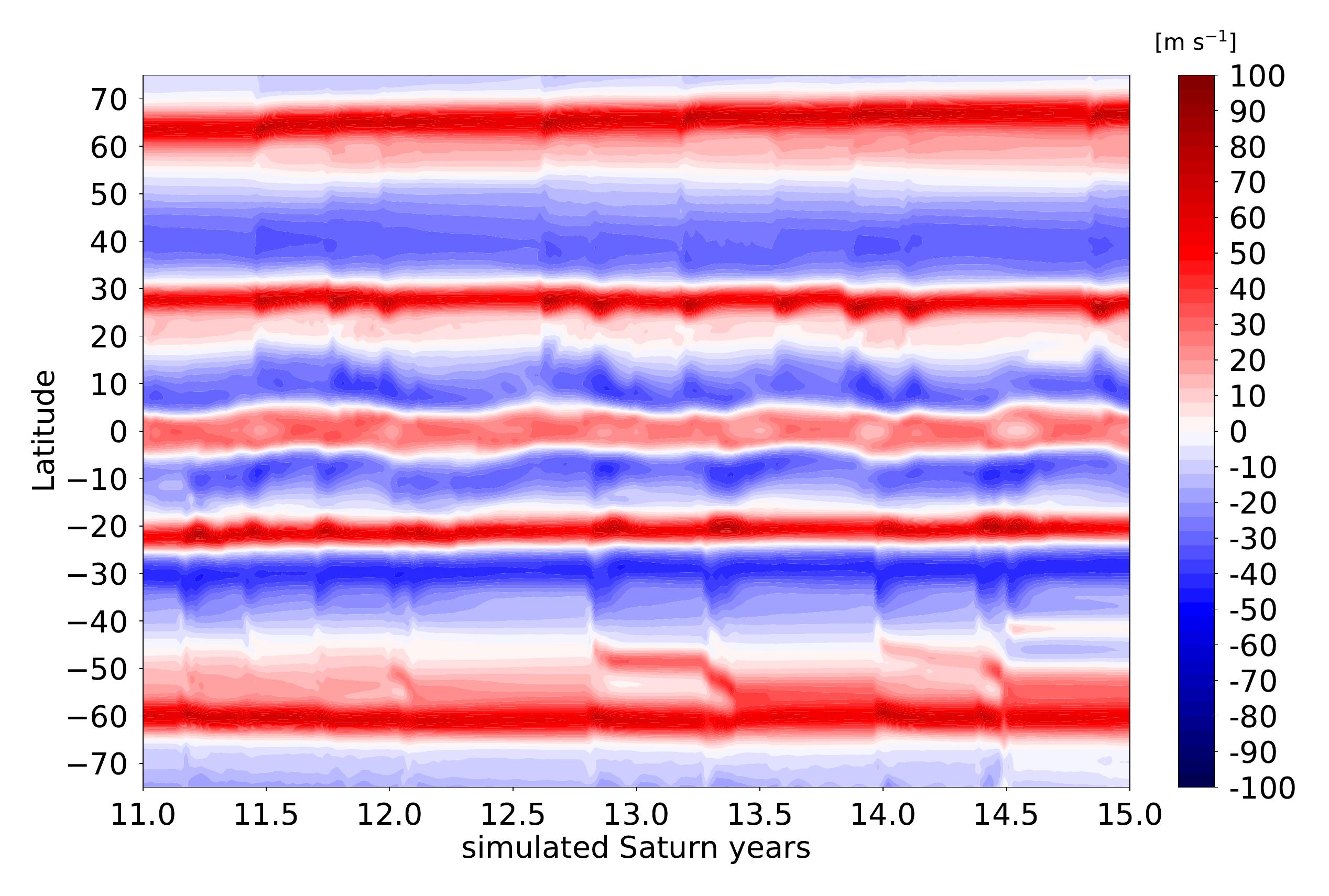
The poleward migration of the mid-latitude jets continues until the migration rate slows down and the zonal jets reach their final latitude of occurrence in our Saturn DYNAMICO GCM simulation. Starting from the seventh simulated year to the fifteenth simulated year (Figures 13 top and 14 bottom), we notice a continuing, very slow poleward migration of the mid-latitude eastward jets and equatorward migration of the tropical jets. The 15-year duration of our Saturn DYNAMICO GCM simulation allows us to reach robust conclusions about the overall steady-state jets’ structure and intensity; the long duration of our simulations also allows us to conclude that this jet structure is still impacted by a slowly-evolving transient state over timescales of tens of Saturn years. It is important to note here that we are not interpreting our Saturn GCM simulations as indicative of a current migration of Saturn zonal jets, which is not supported by observations. Our GCM simulations start with a zero-wind state which is not encountered in the actual Saturn’s atmosphere, and may have never been encountered in the past history of Saturn’s atmosphere. Thus, we can only speculate that jet migration could have been an important process in the past evolution of Saturn’s atmosphere and might explain the present latitudes of Saturn’s zonal jets.
The bursts of eddy activities are also associated with acceleration of the zonal jets, would it be a case of a migration episode or not (once the jets have migrated, the impact of the eddies is actually solely jet acceleration and no longer migration). This suggests that eddy forcing plays a great role in shaping the zonal jets in Saturn’s atmosphere, as argued by existing modeling studies (Showman,, 2007; Lian and Showman,, 2010; Liu and Schneider,, 2010) and Cassini observations (Del Genio et al.,, 2007; Del Genio and Barbara,, 2012). We discuss this matter in section 4.2 for a global analysis and section 4.3 for a local analysis. Despite our Saturn DYNAMICO GCM resolving the seasonal evolution of Saturn’s troposphere and stratosphere, there is no clear seasonal trend associated with the bursts of mid-latitude eddy activity (although the typical timescale between the bursts is close to one year). This is in line with theoretical studies supporting abrupt stochastic transitions in the zonal jet structure prone to barotropic and baroclinic instabilities (Bouchet and Simonnet,, 2009; Bouchet et al.,, 2013). The typical timescale between bursts is not so much set by the seasonal cycle, but by the typical life cycle of instabilities (Panetta,, 1993).
4.2 Kinetic energy conversion rate
To investigate the mechanism by which zonal banded jets arise in our Saturn DYNAMICO GCM simulation, we first consider a global diagnostic, the conversion rate of eddy-to-mean kinetic energy. Cloud tracking with Cassini Imaging Science Subsystem (ISS) images has been employed to address the driving of Saturn’s zonal jets by eddy momentum fluxes (Del Genio et al.,, 2007; Del Genio and Barbara,, 2012). The conversion rate in m2 s-3 (or W kg-1), estimating the conversion per unit mass of eddy kinetic energy to zonal-mean kinetic energy, can be obtained by multiplying eddy momentum transport by the meridional curvature of the zonal flow .
| (8) |
Wind observations by cloud tracking exhibit a globally positive conversion rate , both at the middle troposphere ammonia cloud at bar and the upper troposphere haze at mbar, which suggests that Saturn’s zonal jets are eddy-driven (Del Genio and Barbara,, 2012). The fact that is positive means that the eddy flux is, on average, equatorward in cyclonic shear regions and poleward in anticyclonic shear regions (Del Genio and Barbara,, 2012), hence eastward jets are accelerated by the convergence of eddy flux while westward jets are decelerated by the divergence of eddy flux (see also PV discussions in section 3.2.1). The values of kinetic energy conversion rate observed by Cassini by Del Genio and Barbara, (2012) (their Figure 11) are large: W kg-1 at 100 mbar, and four times larger in the troposphere at 1 bar. Those estimates of the energy conversion rates support the idea that eddy momentum transfers are able to maintain jets against dissipation. Similar conclusions were reached for Jupiter’s weather layer by Salyk et al., (2006).
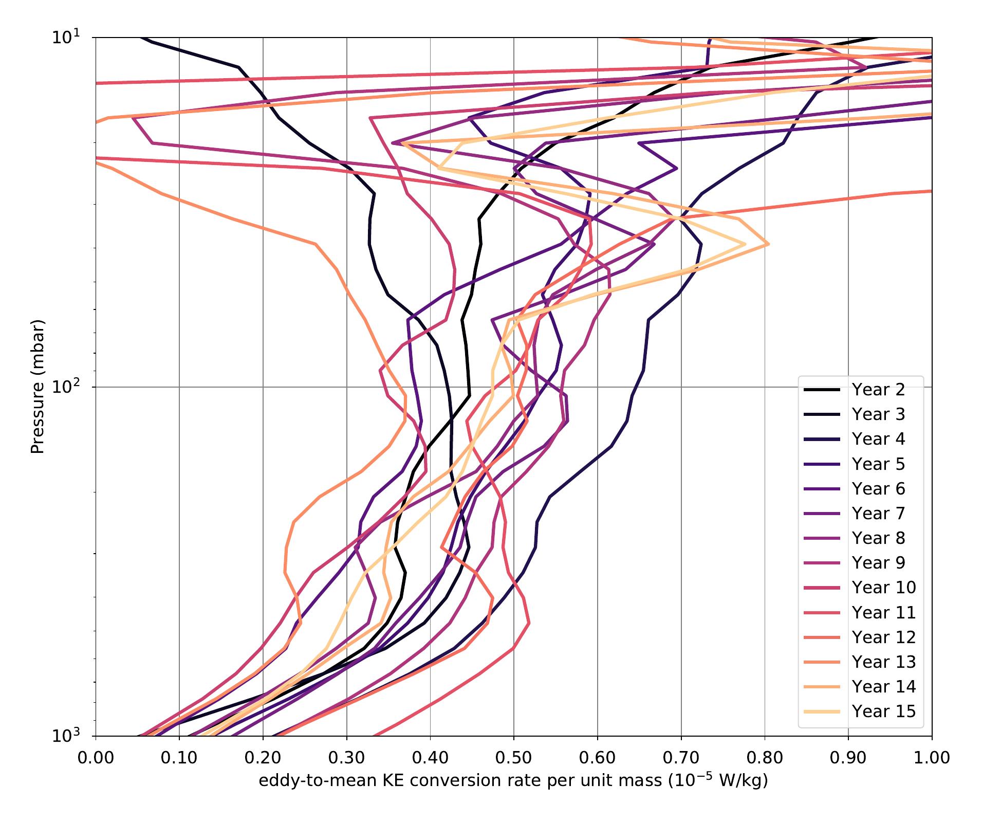
The positive conversion rates simulated by our Saturn DYNAMICO GCM, shown in Figure 16, indicate that our model supports the conclusion of Del Genio and Barbara, (2012) that Saturn’s zonal banded jets are, for a significant part, driven and maintained by eddies in the weather layer (see also Read et al., 2009a, ). This also confirms the diagnostics obtained from previous GCM studies (Lian and Showman,, 2008; Liu and Schneider,, 2010). In the upper troposphere haze layer at hPa, our model predicts m2 s-3, which matches to the order-of-magnitude the quantitative estimates obtained from Cassini by Del Genio and Barbara, (2012), implying a typical timescale of replenishing the jets of less than a Saturn year. This shows that our Saturn DYNAMICO GCM resolves a satisfactory conversion rate from eddies to zonal jets in the tropopause, providing support for a “downward control” of jets at deeper levels (Haynes et al.,, 1991) by eddy forcing in the radiatively-driven upper troposphere, as proposed by Schneider and Liu, (2009) and Liu and Schneider, (2010). Nevertheless, our modeled values for are half those obtained by cloud tracking on board Cassini, indicating room for improvement in predicting the eddy activity and jet curvature resolved by our GCM in the upper troposphere, suggesting the need for either more accurate radiative computations, or an additional physical process causing eddies.
The conversion rate increases with altitude in our Saturn GCM simulation, whereas it decreases with altitude in the Cassini observations of Del Genio and Barbara, (2012). In other words, if our simulations match the observations at 100 mbar, the conversion rate at the cloud layer is one order of magnitude lower in the Saturn GCM simulations than it is in the observations. Del Genio and Barbara, (2012) already noticed this discrepancy by comparing their data to the GCM results of Liu and Schneider, (2010). We speculate that our simulated eddy forcing of jets being compliant with observations in the radiatively-driven tropopause, but not in the deeper troposphere, indicates that a source of tropospheric eddy forcing (e.g. latent heat release and convective motions associated with moist processes Zuchowski et al.,, 2009; Lian and Showman,, 2010) is missing in our Saturn GCM. This is also consistent with our equatorial jet super-rotating too weakly for a possible lack of convectively-generated Rossby waves (Schneider and Liu,, 2009).
4.3 Local analysis of eddy-induced jets
The approach using kinetic energy conversion rate in section 4.2 is to be understood on a global sense; here we present diagnostics for eddy-induced jets that bear a more local sense.
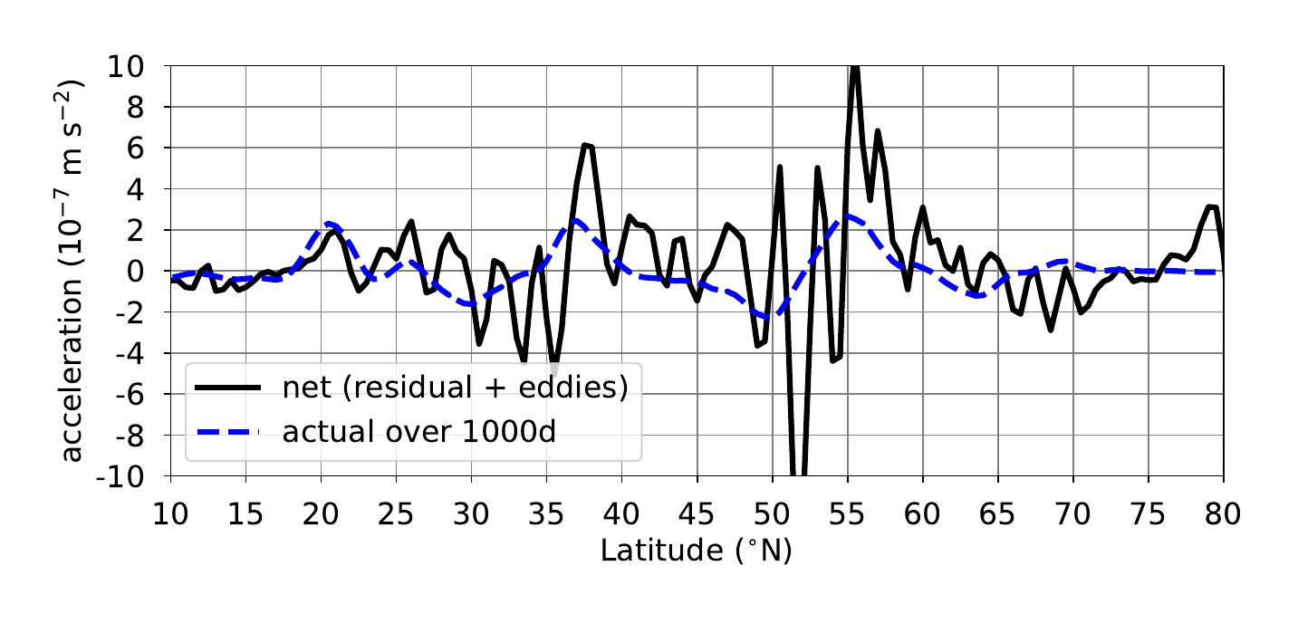
We can consider, as a typical and particularly illustrative example, the impact of the strong burst of eddy activity taking place in the northern hemisphere within 1000 Saturn days between and simulated years (Figure 13). In order to study the contributions to the zonal acceleration, the Eulerian-mean form of the zonal-mean zonal momentum equation of the atmospheric flow motion can be written as follows
| (9) |
where is a mean nonconservative force such as e.g. diffusion, and the respectively “residual-mean” and “eddy-related” terms are written (e.g. equation 2.5 in Andrews et al.,, 1983)
| (10) |
| (11) |
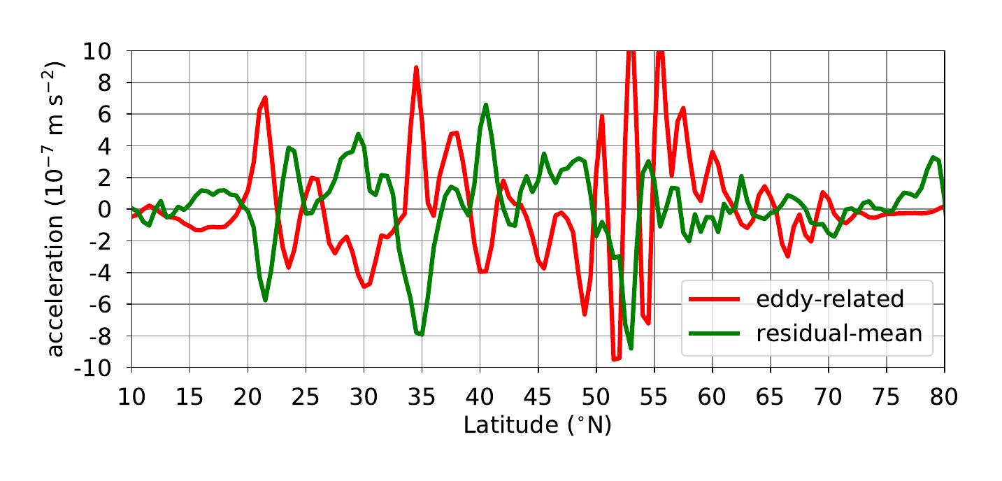
The contributions of each of those terms, within the considered 1000 Saturn days prone to significant eddy activity, are provided in Figure 17. As was also noticed by Lian and Showman, (2008, their Figure 8), the two terms described in equations 10 and 11 are generally anti-correlated, which indicates that a significant part of eddy-related acceleration (which might reach m s-2 on average over 1000 Saturn days) contributes to maintaining an associated meridional circulation, in addition to contributing to the zonal jets. Under the assumption of steady-state zonal jets (), the quasi-equilibrium between eddy-related and meridional-circulation terms is used in studies exploring the circulations underlying observed temperature and aerosol fields in gas giants (e.g., West et al.,, 1992).
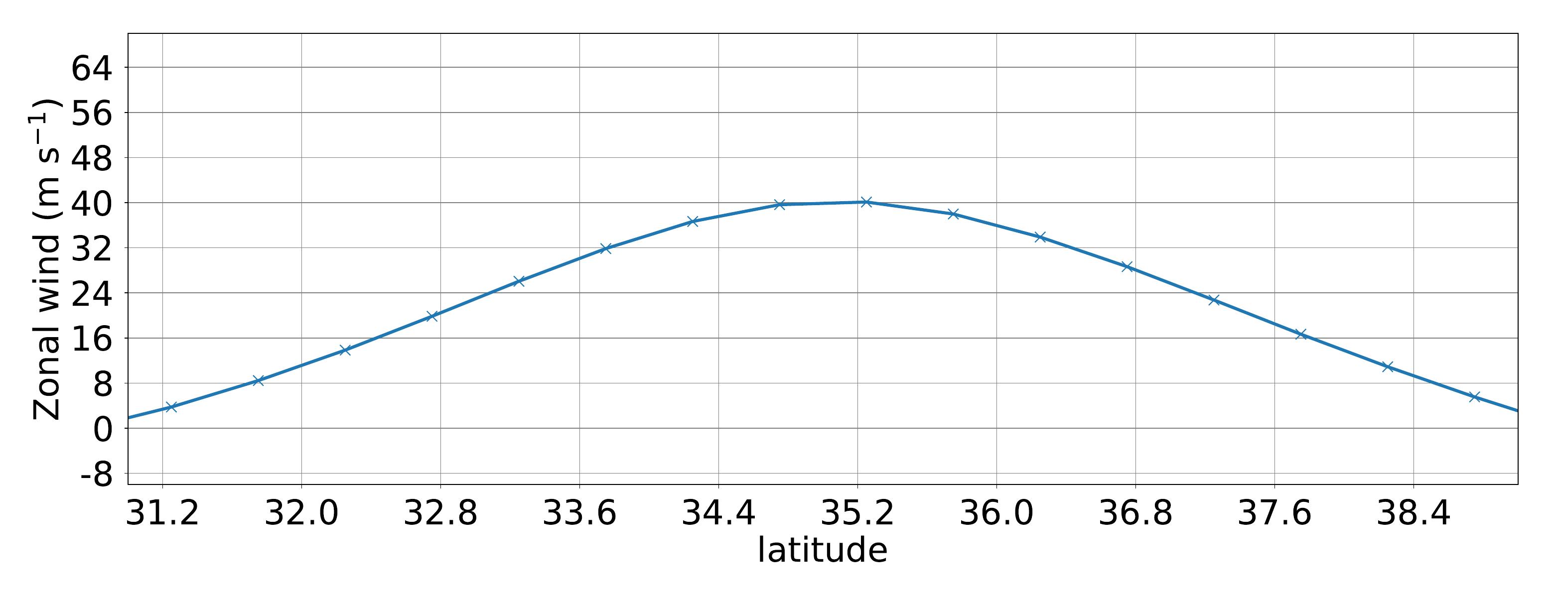
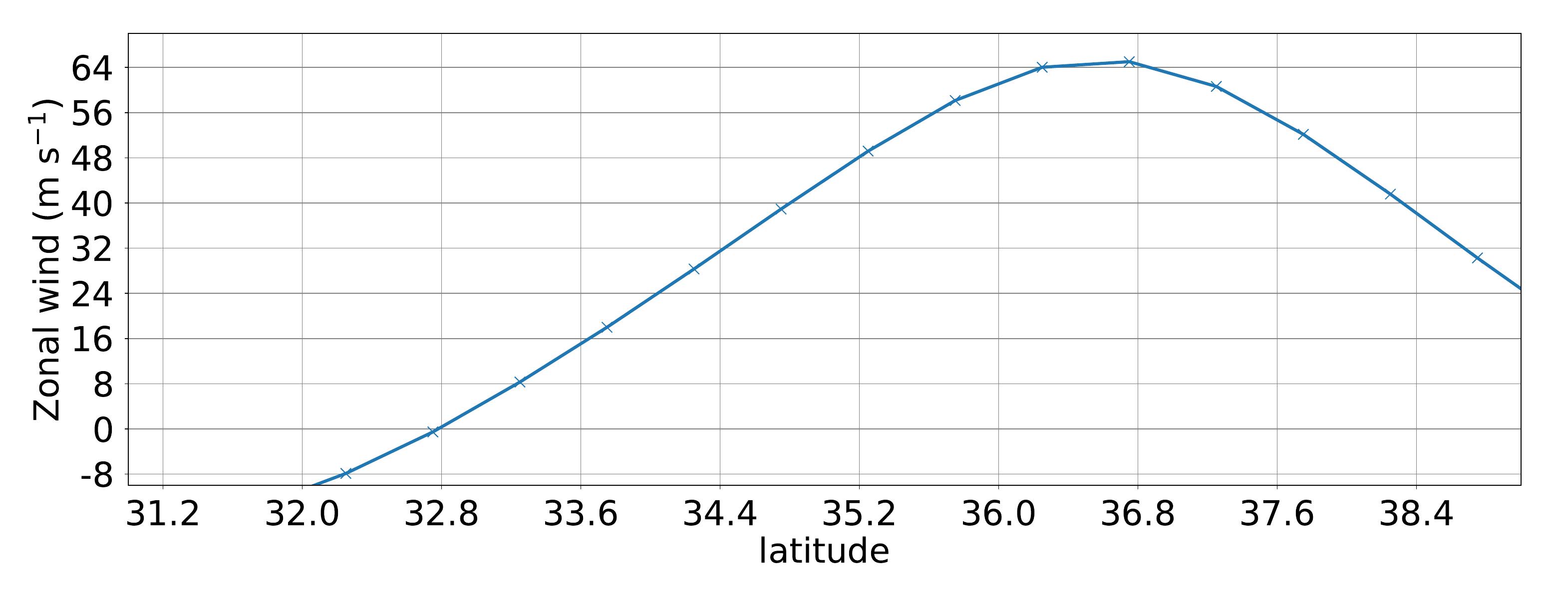
The three northern zonal jets featured in Figure 17 illustrate the possible distinct outcome of local eddy forcing: the N eastward jet is slightly accelerated, in a situation where the residual-mean and eddy-related terms almost compensate; the N eastward jet does not accelerate at its core, but is migrating as a result of an eddy-induced acceleration on its poleward flank; the N eastward jet undergoes strong eddy perturbations, especially on its poleward flank, not compensated by an evolution of the residual-mean circulation, which results in both a poleward migration and an acceleration of this eastward jet. Note that, concomitantly with this overall acceleration of the eastward jets, westward jets are decelerating. This supports the interpretation proposed in sections 3.2.1 and 4.2, and in the literature (e.g., Schneider and Liu,, 2009), that there is a net transfer of momentum from the westward jets towards the eastward jets.
A complementary framework to study the evolution of jets – especially the eddy-related acceleration – is the Transformed Eulerian Mean approach. In this approach, the Eliassen-Palm (EP) flux (e.g., Vallis,, 2006), which meridional component writes in isobaric coordinates (e.g. equation 2.7 in Andrews et al.,, 1983)
| (12) |
provides a direct link between the convergence / divergence of eddy momentum and the resulting acceleration / deceleration of zonal jets. The horizontal contribution of eddies to zonal-mean wind acceleration is the divergence of the meridional component of the EP flux
| (13) |
(The vertical contribution of eddies to zonal-mean wind acceleration is omitted in this equation because, in the specific context of our analysis of eddy-driven jets, it was found to be negligible).We use the expression in equation 12 to diagnose the eddy-driven acceleration in our Saturn GCM simulations; we note, however, that the approximate expression in parenthesis (used e.g. to interpret Figure 8 in section 3.2.2) is reasonable in a vertically-integrated quasi-geostrophic framework, with zonal averaging making mean momentum flux convergence terms to be small compared to the eddy momentum flux convergence terms (Hoskins et al.,, 1983; Vallis,, 2006; Chemke and Kaspi, 2015a, ).
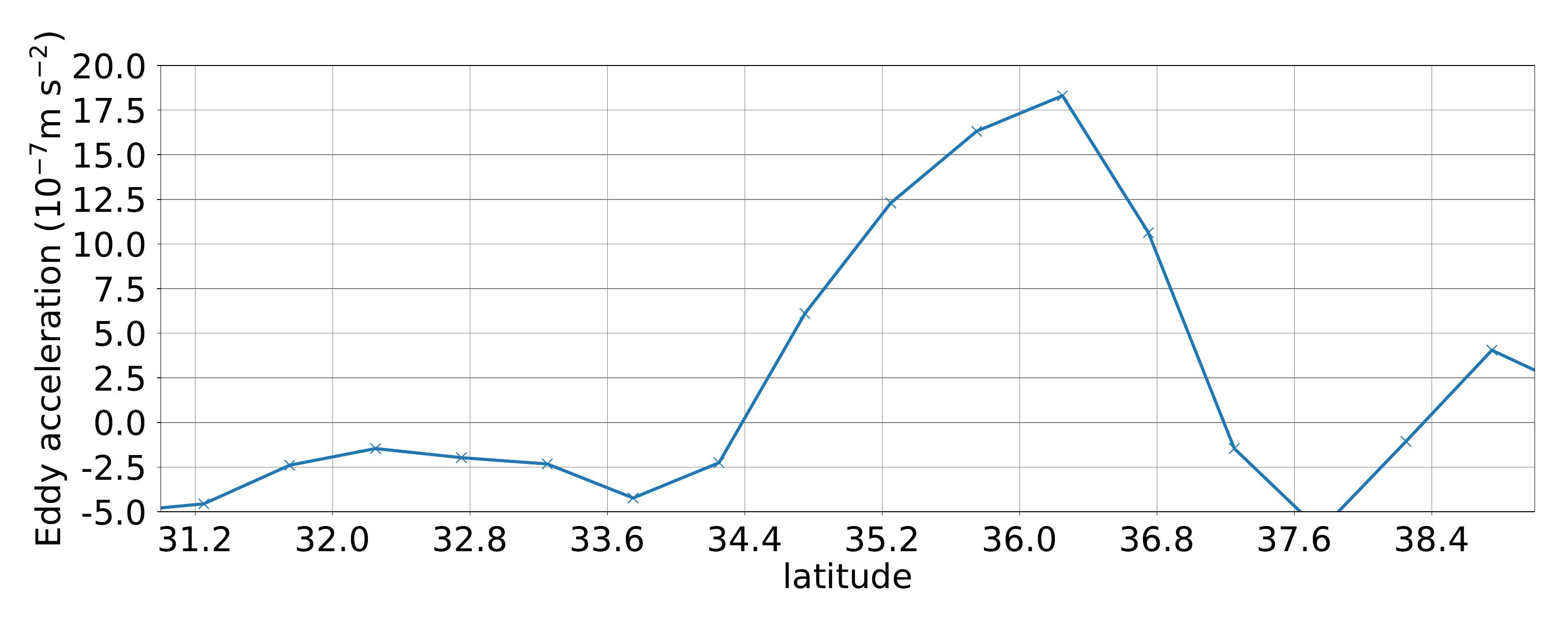
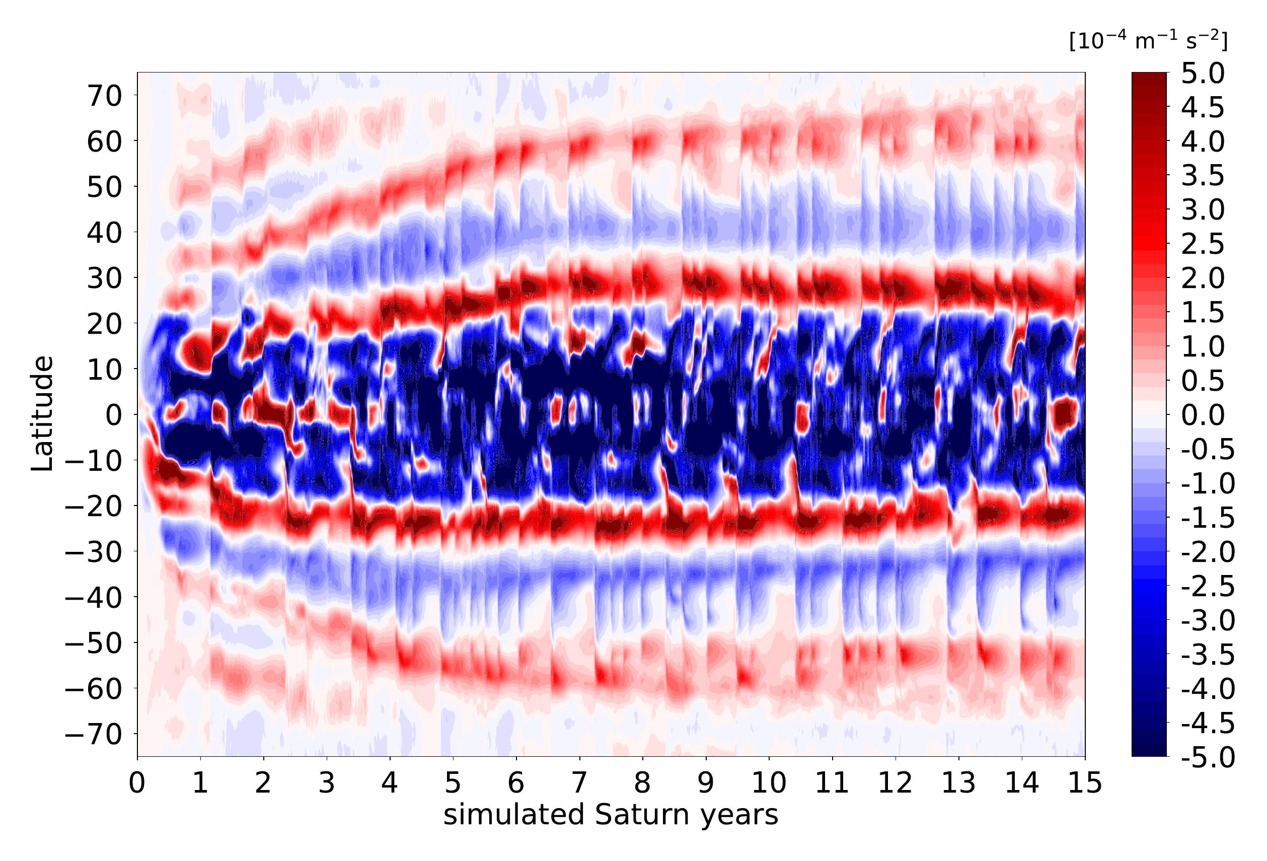
As was found from analyzing Figure 17, the N eastward jet in the end of the first simulated year typically undergoes a poleward migration associated with a burst of eddy activity; this eddy-driven migration is continuing in the beginning of the second simulated year. Figure 18 indicates that the divergence of the Eliassen-Palm flux associated with this eddy activity indeed acts to slow down the jet core and accelerate its flanks, with a larger acceleration being experienced in the poleward side.
4.4 Barotropic vs. baroclinic instability of the jets
The importance of barotropic and baroclinic instabilities has been discussed in the existing literature as the source for gas giants’ banded jets (Dowling,, 1995; Liu and Schneider,, 2010) and the evolution thereof, notably migration (Williams,, 2003; Chemke and Kaspi, 2015a, ). Just as the vertical gradient of potential temperature enables to assess convective instability, the meridional gradient of potential vorticity enables to assess barotropic / baroclinic instability (Dowling,, 1995; Holton,, 2004; Vallis,, 2006). The Rayleigh-Kuo [RK] necessary condition for barotropic instability is that the meridional gradient of PV
| (14) |
changes sign in the domain interior. The Charney-Stern-Pedlosky [CSP] necessary condition for baroclinic instability is that the full-baroclinic meridional gradient of PV
| (15) |
either: changes sign in the interior [CSP1, similar to RK], is the opposite sign to at the upper boundary [CSP2], is the same sign as at the lower boundary [CSP3], or is zero and is the same sign at both boundaries [CSP4]. The CSP criterion is not defined in a neutral layer (where ) such as Saturn’s troposphere, thus we carry out the analysis of the two necessary conditions in equations 14 and 15 near the tropopause level in our simulations.
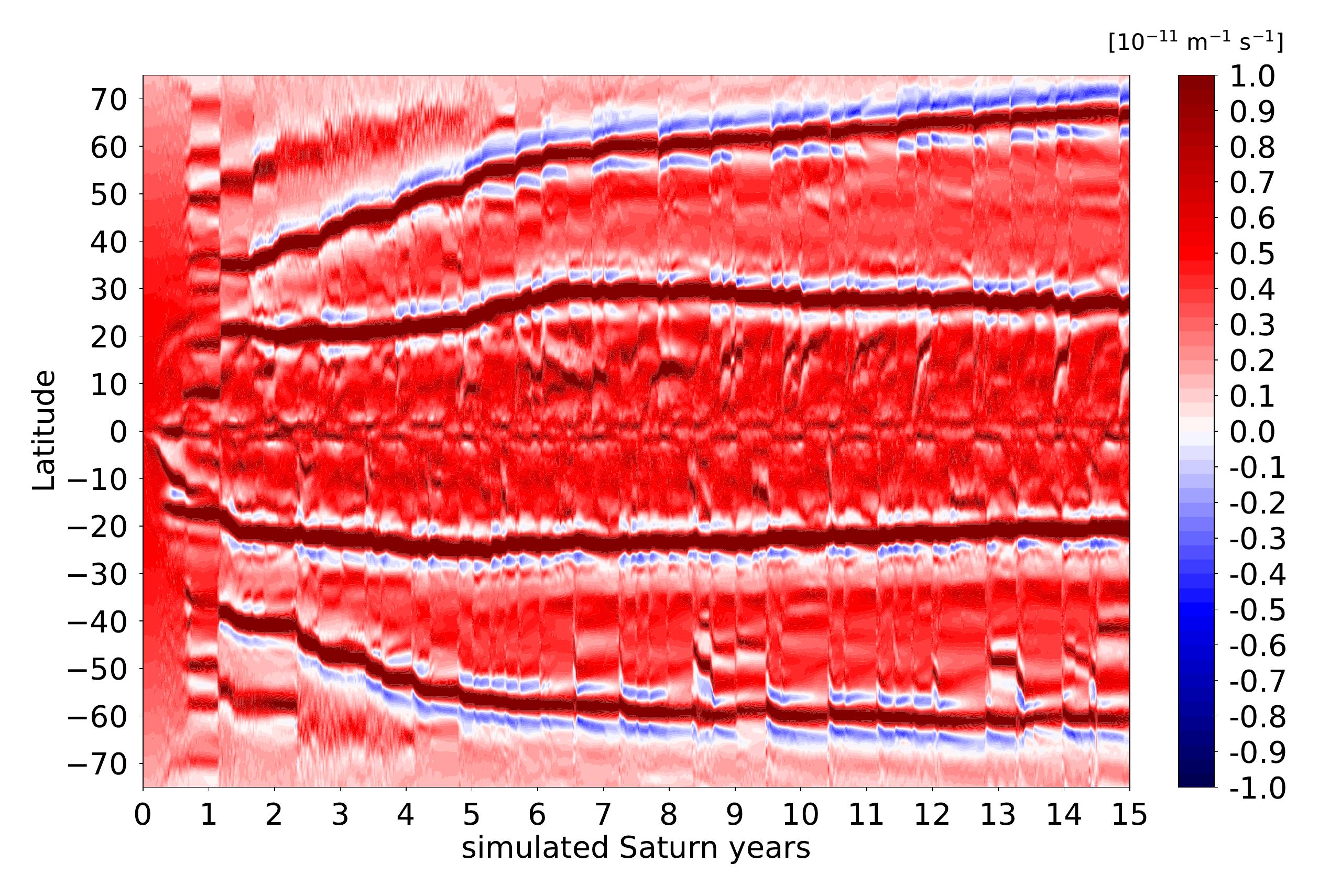
The necessary condition RK for barotropic instability can be assessed from Figure 19 by determining when the quantity described by equation 14 changes sign. In the first four simulated years, the mid-latitude eastward jets migrating from N/S to N/S fulfil the RK condition on the poleward flanks, but not on the equatorward flank. In subsequent years (from year 5 to year 15) in our Saturn DYNAMICO GCM simulations, those eastward jets fulfil the RK on both flanks, which is also the case for the weakly-migrating N/S jets throughout the 15-year simulation. The simulated mid-latitude jets in our Saturn DYNAMICO GCM are thus possibly impacted by barotropic instability; this could be expected from the PV mapping in Figure 12 which clearly shows that strong inversions of the meridional gradients of PV are found at the location of the eastward jets. This provides an explanation for the extratropical eddies found in the bulk of eastward jets and discussed in section 3.3.2. It is worth reminding here that barotropic instability acts to transfer momentum from jets to eddies, and not the contrary. Hence the positive conversion rate indicating an overall transfer from eddies to jets (section 4.2) hints at baroclinic instability complementing barotropic instability.
Referring to the CSP1 criterion, Figure 19 shows that the conditions for baroclinic instability are met in polar regions – this is also true for barotropic instability according to the RK criterion. In mid-latitude eastward jets, the CSP1 necessary criterion for baroclinic instability is however only verified in the poleward flank of the jets; the quantity described in equation 15 is mostly positive at all latitudes (outside polar regions). The fact that the CSP1 criterion for baroclinic instability is fulfilled in the poleward flank of the mid-latitude jets, and less so in the equatorward flank, echoes the conclusions of Chemke and Kaspi, 2015a who demonstrated that the poleward migration of jets in idealized GCM simulations of high-rotation planets is caused by a poleward bias in baroclinicity across the width of the jet.
The condition CSP3 is fulfilled in the simulated mid-latitude eastward jets since the (baroclinic) meridional gradient of PV is of the same sign as the vertical shear , i.e. positive as is shown in Figure 19 (see also section 3.2.1). Those simulated jets could thus be baroclinically unstable111CSP3 is often the decisive condition in the terrestrial environment too, see Vallis, (2006). An assessment of conditions CSP 2 and CSP 4 in the case of our Saturn DYNAMICO GCM simulations indicates that those are not fulfilled.. This is not the case for the equatorial eastward jet, and the broad westward jets, for which vertical shear is negative.
We conclude that both barotropic and baroclinic instabilities could account for the maintenance, migration and (in polar regions) disappearance of eastward zonal jets in our Saturn DYNAMICO GCM simulations. The putative role of baroclinic instability in driving the mid-latitude jets was also highlighted by Liu and Schneider, (2010); the possibility that barotropic and baroclinic instabilities exist in Saturn’s troposphere is also argued in Studwell et al., (2018). In that respect, the pole-to-equator meridional gradient of temperature in the deep troposphere (e.g. at pressures greater and equal to 500 mbar) is a key constraint for baroclinic instability, owing to its link to the vertical shear of zonal wind involved in the CSP3 criterion, through the thermal wind equation.
The equator-to-pole temperature gradient of 4 K found at the 500-mbar level in Figures 2 and 3 (bottom) translates into about 7 K at the 2.5-bar level, in accordance with potential temperature being constant in the neutral lower troposphere. Both correspond to an equator-to-pole gradient of potential temperature of 7 K. As is discussed in section 3.1, while a good agreement between our model and the observations is obtained in the upper troposphere / lower stratosphere (Figure 4), the simulated baroclinicity in the lower troposphere is at least twice larger than it is in the observations. In addition to this, the shallowness of our Saturn GCM (as well as other models sharing the same strategy, e.g. Liu and Schneider,, 2010) prevents it from resolving the deep large-scale circulations that could act to counteract and further homogenize the meridional gradients of potential temperature in the deeper troposphere (Aurnou et al.,, 2008). According to the CSP3 criterion, an unrealistic baroclinicity at the bottom boundary entails that part of the eddies resolved by our Saturn DYNAMICO GCM could be spurious and not occurring in the real Saturn – contrary to the baroclinicity associated with PV gradient reversals within the atmospheric fluid related to the CSP1 criterion. This would impact the structure of the resolved zonal jets, as well as their meandering and migration. A similar word of caution applies to the analysis of the conversion rate in Figure 16 and section 4.2, even if the order of magnitude compared to observations is correct. For instance, the fact that baroclinic instabilities cause unrealistically strong jet meandering in polar regions may be deemed an indication that meridional gradients could be improved at the bottom of our model. Deepening the model bottom and ensuring a more realistic baroclinicity in the lower troposphere is an area of future improvement of our Saturn DYNAMICO GCM, as is the case for most existing shallow-atmosphere models.
5 Conclusions
The conclusions of our study can be summarized as follows.
-
1.
The Cassini mission opened novel questions on tropospheric and stratospheric circulations on Saturn, with new modeling challenges (section 1 and challenges ).
- 2.
-
3.
Care must be taken when developing a GCM for gas giants in setting the subgrid-scale dissipation and verifying the conservation of global axial angular momentum (appendix A).
-
4.
We reached the capability to simulate the dynamics of Saturn’s atmosphere from the troposphere to the lower stratosphere during 15 Saturn years with an horizontal resolution of longitude / latitude, which made our reference simulation (sections 3 and 4); our Saturn DYNAMICO GCM produces a satisfactory thermal structure, and seasonal variability thereof, compared to Cassini CIRS measurements (section 3.1).
-
5.
The number and intensity of mid-latitude eastward jets (and broad westward jets) reproduced by the reference GCM simulation is compliant with observations, although slightly underestimated, but no stable circumpolar jet (less so hexagonal-shaped) is reproduced; those jets’ intensities increase with altitude and their latitudinal organization exhibits potential-vorticity staircases (section 3.2.1).
-
6.
The GCM simulation exhibits at the equator both a superrotating zonal jet in the troposphere and stacked alternating zonal jets in the stratosphere; nevertheless, the former is one order of magnitude less powerful than the observed jet, and the latter are not downward-propagating with time as would be expected from the observed equatorial oscillation (section 3.2.2).
-
7.
Our model produces a wealth of Yanai (Rossby-gravity), Rossby and Kelvin waves in the tropical channel, part of them hinted at in available observations (section 3.3.1).
-
8.
Outside the tropics, the cores of eastward jets are perturbed by Rossby waves reminiscent of Ribbon-like waves, while westward jets host an eddy activity not especially organized in vortices, which transitions in polar regions into a predominance of large-scale vortices (section 3.3.2).
-
9.
In the 15-Saturn-year course of our Saturn DYNAMICO GCM simulation, eastward jets undergo poleward migration and perturbations by bursts of eddies (section 4.1).
-
10.
The global kinetic energy conversion rate simulated in our Saturn DYNAMICO GCM, albeit half the value of the observed estimates, is positive and argues for a significant contribution of eddy acceleration in driving the eastward jets (section 4.2).
-
11.
The acceleration (and, if applicable, migration) of jets caused by eddy momentum transfers is evidenced by local analysis with either Eulerian-mean or transformed Eulerian-mean formalism (section 4.3).
-
12.
Eastward jets produced by our Saturn DYNAMICO GCM are prone to both barotropic and baroclinic instabilities (section 4.4).
Based on the present study, and the comparison between available observations and our GCM simulations, we can envision the following improvements of our Saturn DYNAMICO GCM in the future:
-
to refine the horizontal resolution to ;
-
to include a physically-based parameterization for subgrid-scale dry and moist convection, and to subsequently deepen the model bottom to 10-20 bars;
-
to extend the model top to the upper stratosphere and to refine the vertical resolution in the troposphere and the stratosphere;
-
to implement a parameterization for the impact of unresolved mesoscale gravity waves on the mean flow.
This list is not exhaustive, but represents the near-future evolution of our model. Long-term developments would be inspired by the model-coupling methodology for the climate of telluric planets, i.e. coupling our Saturn DYNAMICO GCM with stratospheric photo-chemical models, deep-interior convection models and upper-atmosphere thermo-iono-spheric models.
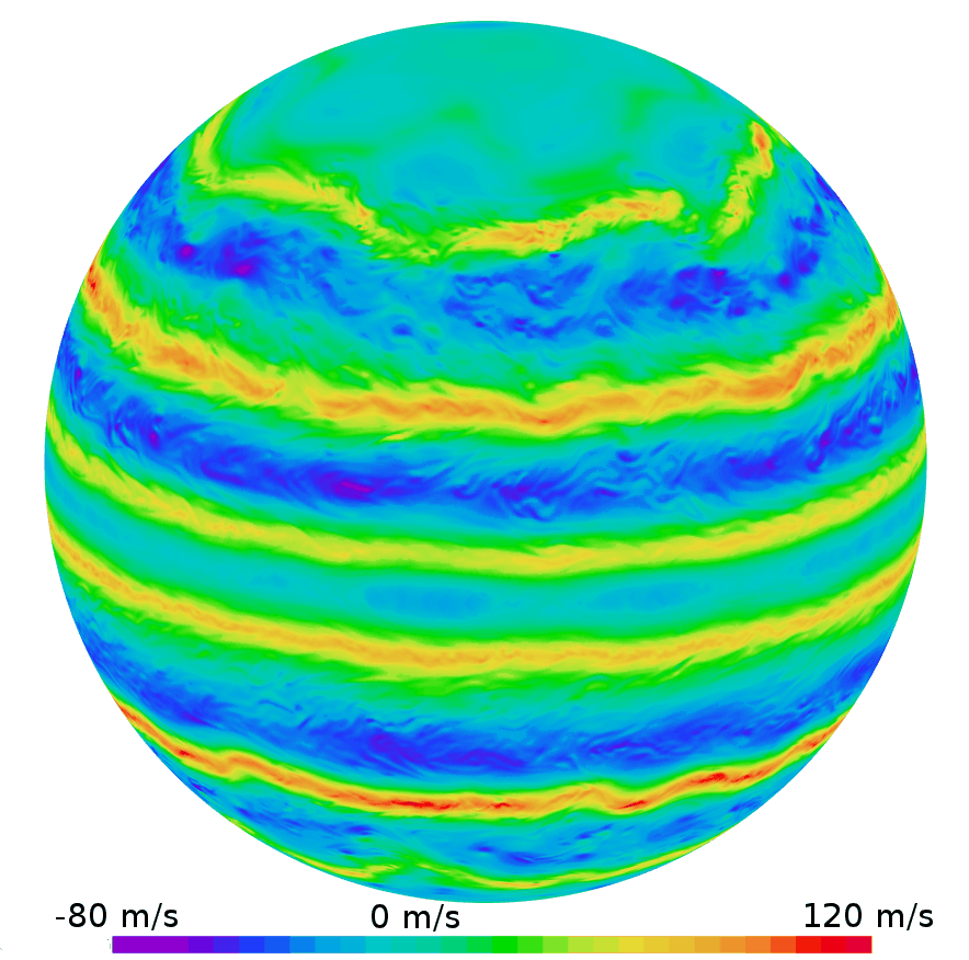
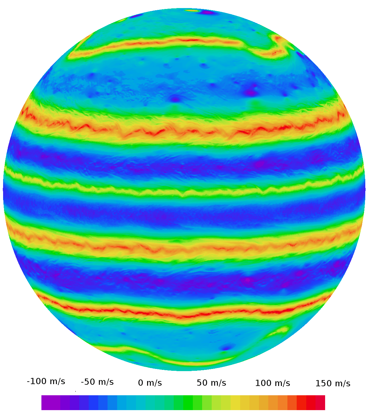
What the refinement of horizontal resolution would bring to Saturn GCM studies can be illustrated by the tests of an earlier version of the Saturn DYNAMICO GCM at the horizontal resolutions of and . We carried out overdissipated GCM simulations at those resolutions, using both a sponge layer and hyperdiffusion timescales of the order s, to ensure overly-conservative numerical stability in order to test the performance of the model on massively-parallel architectures (up to cores). Those simulations are thus not optimized for scientific return222This is all the more true since the outcome of a 2-Saturn-year simulation at (hence not fully spun-up) was used to initialize a simulation, and similarly from the to the simulations and the approach described in appendix A will have to be carried out again in the future for the and configuration of the model. Yet, even those imperfect and simulations with the Saturn DYNAMICO GCM demonstrate the potential of the model to better resolve eddies, waves and vortices with refined horizontal resolution, as is shown in Figure 20 and in the movie included as supplementary material, showing wind amplitude and vorticity from the Saturn DYNAMICO simulation.
Finally, we note that the Saturn DYNAMICO GCM is only a first step towards a GCM system able to simulate the atmospheres of all giant planets, ice giants Uranus and Neptune included. The development of the Jupiter DYNAMICO GCM is currently ungoing (Guerlet and Spiga,, 2016; Boissinot et al.,, 2018), along the lines drawn for Saturn by Guerlet et al., (2014) and this study. The similarities and differences between Jupiter and Saturn in their banded jets (Ingersoll,, 1990; Dowling,, 1995; Kaspi et al.,, 2018), eddy activity (Salyk et al.,, 2006) equatorial oscillations (Li and Read,, 2000; Simon-Miller et al.,, 2007), large-scale vortices (Youssef and Marcus,, 2003; Fletcher et al., 2010b, ; Simon et al.,, 2014; Legarreta and Sánchez-Lavega,, 2005) relate to fundamental research in geophysical fluid dynamics. Employing GCMs for giant planets could help, along with observations, to reach a detailed understanding of the big picture of giant planets’ climate and meteorology. This is all the more relevant to prepare the next round of observations of the giant planets, with either probes (Mousis et al.,, 2014), telescopes (Norwood et al.,, 2014), or orbiting spacecraft (Cavalié et al.,, 2017).
Acknowledgments
The authors thank the editor Darrell Strobel, an anonynous reviewer and Adam Showman for extremely constructive reviews which helped to improve the manuscript. We would like to thank Tapio Schneider, Yohai Kaspi, Leigh Fletcher, Glenn Orton, Roland Young, Peter Read, Mike Flasar, François Forget, Michel Capderou, Pierre Drossart, Thibault Cavalié, Agustin Sanchez-Lavega, Ricardo Hueso, Thérése Encrenaz, Emmanuel Lellouch, Frédéric Hourdin, Sébastien Fromang, for useful discussions and questions on preliminary versions of the work reported in this paper.
The authors acknowledge exceptional computing support from Grand Équipement National de Calcul Intensif (GENCI) and Centre Informatique National de l’Enseignement Supérieur (CINES). All the simulations presented in this paper were carried out on the Occigen cluster hosted at CINES. This work was granted access to the High-Performance Computing (HPC) resources of CINES under the allocations 2015-017357, 2016-017548, A001-0107548, A003-0107548, A004-0110391 made by GENCI. We also thank CINES for a “Grand Challenge” exceptional allocation in early 2015 to test the performances of the Saturn DYNAMICO GCM at various horizontal resolutions.
Dubos, Cabanes, Spiga, Meurdesoif, Millour acknowledge funding from Agence Nationale de la Recherche (ANR), project HEAT ANR-14-CE23-0010. Guerlet, Indurain, Spiga acknowledge funding from Agence Nationale de la Recherche (ANR), project OMAGE ANR-12-PDOC-0013. Spiga, Cabanes, Guerlet acknowledge funding from Agence Nationale de la Recherche (ANR), project EMERGIANT ANR-17-CE31-0007. Guerlet, Spiga, Lebonnois acknowledge funding from Centre National d’Études Spatiales (CNES) project exploiting CIRS measurements onboard Cassini. Boissinot, Spiga acknowledge funding from Region Île-de-France DIM ACAV+ project JOVIEN. Sylvestre, Fouchet, Spiga acknowledge funding from Université Pierre et Marie Curie (now Sorbonne Université) Émergence program. Leconte acknowledges that this project has received funding from the European Research Council (ERC) under the European Union’s Horizon 2020 research and innovation program (grant agreement No. 679030/WHIPLASH).
Appendix A Impact of assumptions in the dynamical core
Numerical subgrid-scale dissipation in the model was found to be a critical setting to deal with. The sensitivity of simulated jets with horizontal dissipation is a common issue in GCM: it was specifically discussed for the cases of Venus (Lebonnois et al.,, 2013), Titan (Newman et al.,, 2011), and hot Jupiters (Thrastarson and Cho,, 2011). This is a particularly important issue for a gas giant GCM, and it is discussed in section A.1. Another important question is to explore the behaviour of global axial angular momentum in our Saturn DYNAMICO GCM simulations, which is done in section A.2.
As far as the sensitivity of the modeled jets to the settings adopted for bottom drag is concerned, we rely on the work by Liu and Schneider, (2010) and Liu and Schneider, (2011), and adopt their settings Earth days and for our reference simulation. Simulations with Saturn DYNAMICO carried out with different values of those parameters (respectively Earth days and ) confirm the conclusions of Liu and Schneider, (2010) and Liu and Schneider, (2011) that the bottom drag affects the jets’ width and speed.
A.1 Exploring the impact of dissipation
A subgrid-scale dissipation term is included in our Saturn DYNAMICO GCM to prevent the accumulation of energy at scales close to the grid resolution, caused by the GCM not resolving the turbulent scales at which this energy is dissipated. This hyperviscosity term is written in our Saturn DYNAMICO model as an iterated Laplacian term on a given variable
| (16) |
where is the order of dissipation and the damping timescale associated with the variable at the smallest spatial scale resolved by the model for a given horizontal discretization. Large values of means weaker dissipation: is the times it takes to dissipate a perturbation on variable developing at the spatial scale . The three variables denoted by are vorticity, divergence, and potential temperature, chosen to set horizontal dissipation on respectively the rotational component of the flow (e.g. Rossby waves), the divergent component of the flow (e.g. gravity waves), and the diabatic perturbations (e.g. coming from the physical packages). In GCMs for telluric planets, strong variations from one grid point to one another result from topography contrasts or mesoscale convective cells, which calls for a preferential damping on the divergent flow (Hourdin et al.,, 2012). In our Saturn DYNAMICO GCM simulations, we adopt a simpler approach and we set the same dissipation rate for all three variables, namely for divergence, vorticity and potential temperature.
In the GCM methodology, suitable values of are determined empirically, using a combination of past modeling experiences and trial-and-error approach using GCM simulations. The “right” settings for numerical dissipation is a trade-off between ensuring model stability, damping energy at the smallest resolved scales, and minimizing impact on the large-scale flow. A common practice is ranging between and , and typically one-two terrestrial hours ( s) for a GCM simulation. We chose (fourth-order dissipation) for the Saturn DYNAMICO GCM simulations, since it is the setting adopted by our team for GCM for telluric bodies (Hourdin et al.,, 1995; Lebonnois et al.,, 2010), and because is overly dissipative on circulations at large scales, while led to results similar to . We then carried out several one-Saturn-year simulations with our Saturn DYNAMICO GCM to explore the sensitivity of the computed tropospheric jet structure to the dissipation timescale .
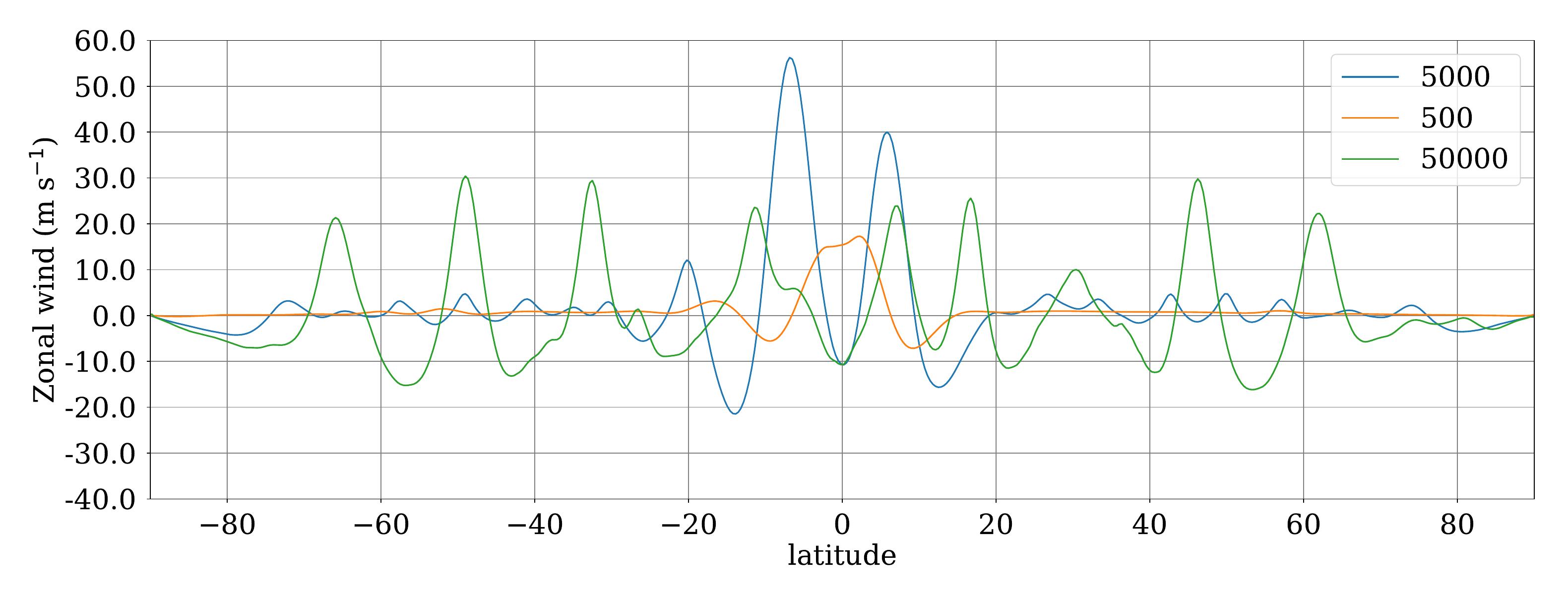
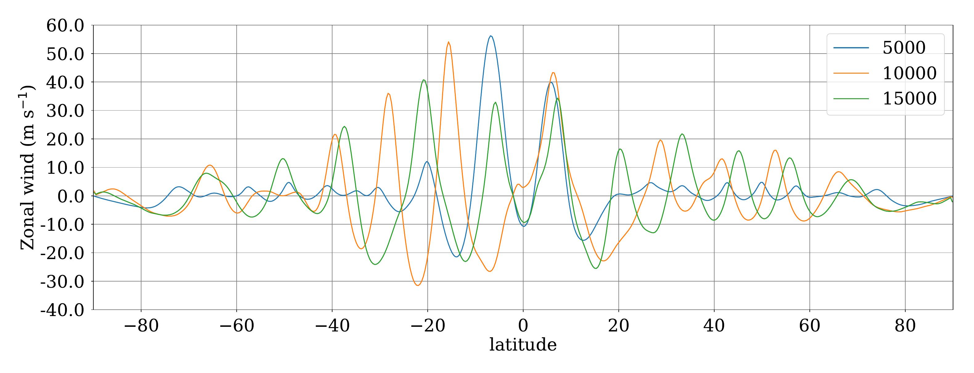
Figure 21 shows that the simulated tropospheric jets in our Saturn DYNAMICO GCM simulations are sensitive to the value assumed for dissipation timescale . A first order-of-magnitude sensitivity study (Figure 21, top) using extreme values disqualifies the strongest dissipation rate () which damps the mid-latitude jets out of existence. Setting a weak dissipation () lets jets significantly accelerate within one simulated year – before the GCM simulation undergoes numerical instabilities in the second year of simulation. A refined sensitivity study (Figure 21, bottom) indicates that results obtained with or are essentially similar: the choice of dissipation mainly impacts jets’ meridional location.
The selective criterion to choose for our reference Saturn DYNAMICO GCM simulation is then based on observations of Saturn’s jets (Porco et al.,, 2005; García-Melendo et al.,, 2010; Studwell et al.,, 2018) from which we argue that, qualitatively, sets a more realistic velocity profile. With , high and mid latitudes jets are inconsistently weak, while smoothes the prevailing contrast that exists between equatorial and high-/mid-latitude jets. The value of is thus adopted for the 15-year-long reference simulation discussed in sections 3 and 4. It is important to note here that would have been an acceptable choice as well. Figure 21 (right) shows that, even the intensity and location of jets can be different between the Saturn DYNAMICO GCM simulations with either or , the overall jet structure is qualitatively similar in both cases.
To understand why dissipation impacts the jets, it is important to keep in mind that eddies, which putatively drive the jets, have typical length scales of a couple degrees latitude for a grid spacing of (assuming the eddies are baroclinically driven and taking the Rossby radius of deformation as a first-order theoretical estimate of the eddy length scale, e.g. Young and Read,, 2017). These eddies are thus potentially dampened by numerical dissipation that dominantly acts on the smallest-resolved scales. Undoubtedly, the next challenge is to refine GCM resolution towards (or better) to enhance simulations of eddies, and hence planetary jets. Even at such refined horizontal resolution though, the chosen value of will still be impacting the jets’ intensities and locations (see also equation 21 in section A.2). Ultimately, how dissipative the Saturn atmosphere is for small-scale circulations remains an open question and difficult to constrain with observations (Ingersoll et al.,, 2018).
A.2 Angular momentum
The atmospheric Axial Angular momentum (AAM) is defined by the sum of the planetary contribution associated with the solid-body rotation of the planetary sphere and the relative contribution associated with the motions of the atmosphere with respect to the solid-body rotating reference
| (17) |
where denotes global integration over the volume of the atmosphere and denotes the AAM terms per unit mass for respectively the planetary and relative contributions
| (18) |
Thus, the temporal evolution of AAM is either related to atmospheric mass redistribution (that is, the temporal evolution of surface pressure) or wind variability (that is, the temporal evolution of zonal wind). Assuming that hydrostatic primitive equations are considered, and in the absence of any surface torque and zonal mechanical forcing, the globally-integrated AAM is conserved provided the top lid does not vary with longitude (Staniforth and Wood,, 2003; Thuburn,, 2008; Lauritzen et al.,, 2014), which is ensured by the DYNAMICO formulation (Dubos et al.,, 2015).
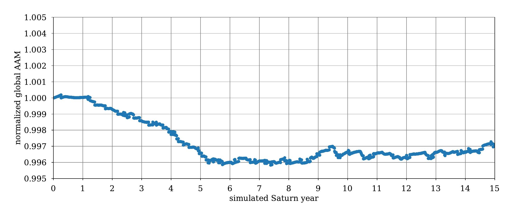
The conservation of global AAM in our Saturn DYNAMICO model is satisfying (Figure 22). There is a very small decrease of global AAM () in the first six simulated Saturn years, which correspond to the dynamical spin-up of our model, before the global AAM stabilizes at a final value and only undergoes negligible temporal variations of the order . The properties of AAM conservation of our Saturn DYNAMICO model compare very favorably to the performance of the dynamical cores described in Polichtchouk et al., (2014), where most models exhibit typical AAM drifts of (reaching several tens of % for one particular model).
In addition to the conservation of global AAM, negligible “AAM noise” must be ensured (Lebonnois et al.,, 2012; Lauritzen et al.,, 2014). How the temporal evolution of global atmospheric AAM splits between each term of the GCM tendencies can be written
| (19) |
where is the AAM tendency associated with subgrid-scale mixing in the physical packages (mostly boundary-layer effects), is the AAM tendency associated with mountain torques, is the AAM tendency associated with upper sponge layer (a reminder that upper-level sponge layer might alter significantly the AAM balance, Shaw and Shepherd,, 2007), is the AAM tendency due to conservation errors in the parameterization of horizontal dissipation, and is a residual numerical rate of AAM variation due to conservation errors (hereinafter named the “AAM noise” since it is a spurious source/sink of AAM in the model). The AAM noise can be diagnosed in a GCM by adding the temporal variations of and computed by the primitive equations () in the dynamical core, excluding any term accounted for in , , or (e.g. explicit diffusion operators are included in )
| (20) |
In the impossible perfect situation where no numerical approximations or errors are made in the GCM dynamical core when solving the primitive equations, the AAM noise should be zero since AAM is exactly transferred from the solid-body rotation to the atmospheric flow and vice versa; a GCM simulation where is of similar or larger magnitude than the other torques would be questionable (Lauritzen et al.,, 2014).
In our Saturn GCM simulations with DYNAMICO, also includes the Rayleigh friction at the bottom of the atmosphere, is zero because no upper-level sponge layer is used, is zero since gas giants are devoid of surface, and for a similar reason, in practice the term is one order of magnitude smaller than other terms. This means that in the case of our Saturn GCM (and more generally for any gas giant GCM) equation 19 reduces to
| (21) |
Hence the angular momentum noise has potentially a strong impact on the temporal AAM variability in a gas giant GCM. A similar concern is raised by Lebonnois et al., (2012) in the case of idealized Venus simulations without topography. The requirement of low AAM noise is less stringent in realistic GCM simulations for Earth, Venus, or Titan where the contribution of mountain torques is large (Lebonnois et al.,, 2012; Lauritzen et al.,, 2014).
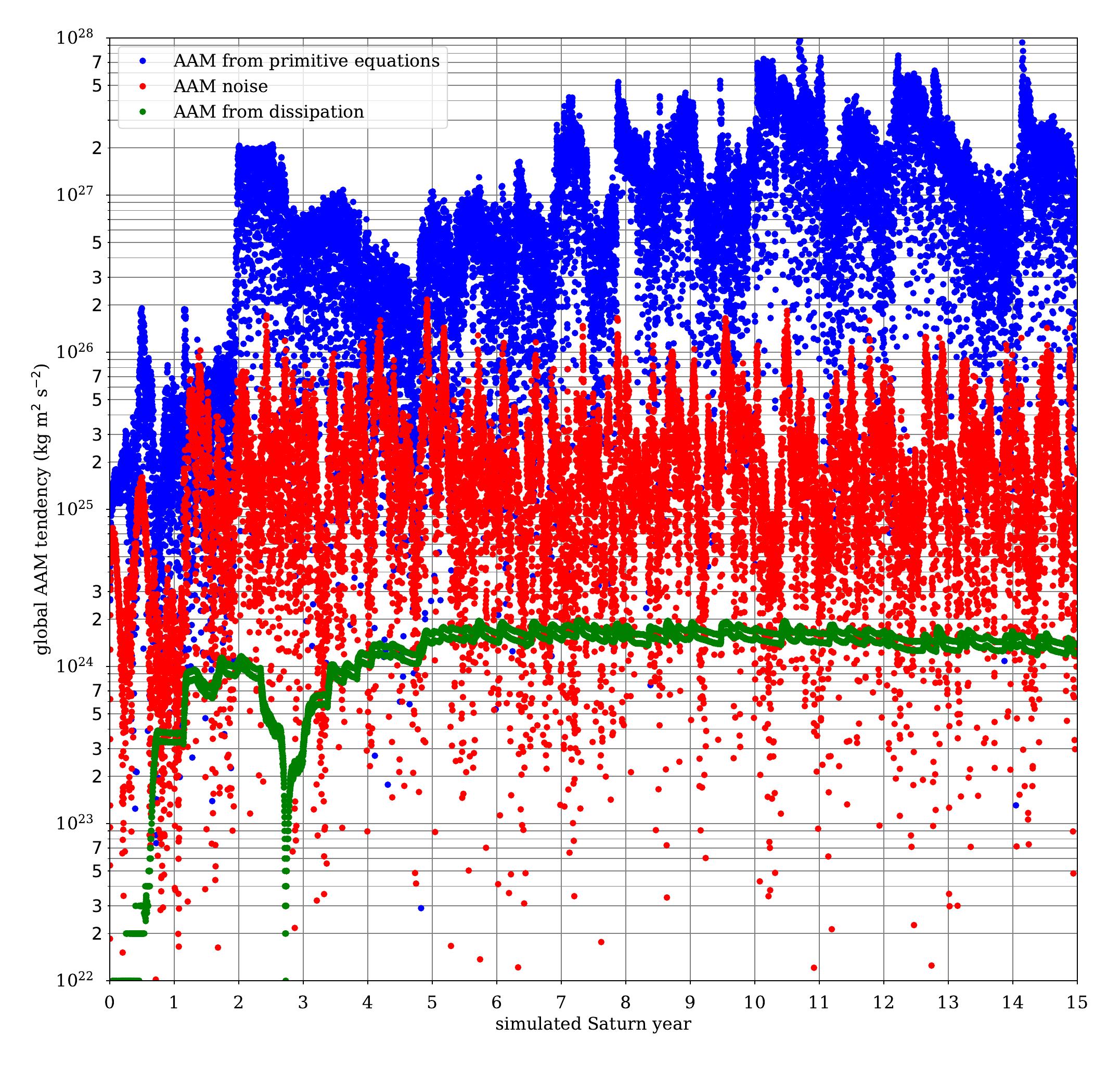
Compared to the analysis presented in Lebonnois et al., (2012) and Lauritzen et al., (2014) for telluric planets, the analysis of AAM noise is more straightforward for gas giants. The following condition333This condition is equivalent to i.e. the gas-giant (simplified) equivalent of the condition in Lebonnois et al., (2012) must be ensured
| (22) |
Figure 23 shows that this condition 22 is fulfilled in our Saturn GCM, with AAM noise being one to two orders of magnitude smaller than AAM tendencies computed in the dynamical core’s primitive equations (except for a short duration close to one and half simulated year). This indicates that AAM noise does not alter the dynamical predictions for jets and eddies. The same conclusion stands for the AAM tendencies associated with dissipation and Rayleigh drag (Figure 23), which are even smaller than the AAM noise. This indicates that the horizontal dissipation set in our GCM (section A.1) has a negligible impact on the AAM budget – this is consistent with the overall jet structure being similar in simulations using either or .
In an attempt to explore the model settings that could influence the AAM noise , we found that it is basically insensitive to time step, vertical discretization, horizontal dissipation (only a very strong horizontal dissipation significantly lowers AAM noise, but adversely impacts the intensity of jets). This is consistent with Lauritzen et al., (2014) conclusions that AAM noise is likely related to small conservation errors associated with the horizontal discretization of primitive equations. The low AAM noise in our Saturn DYNAMICO GCM simulation level ensures that dynamical spin-up of the jets is not due to convergence of numerically-spurious angular momentum.
References
- Achterberg and Flasar, (1996) Achterberg, R. K. and Flasar, F. M. (1996). Planetary-Scale Thermal Waves in Saturn’s Upper Troposphere. Icarus, 119:350–369.
- Andrews et al., (1987) Andrews, D. G., Holton, J. R., and Leovy, C. B. (1987). Middle Atmosphere Dynamics. Academic Press.
- Andrews et al., (1983) Andrews, D. G., Mahlman, J. D., and Sinclair, R. W. (1983). Eliassen-Palm Diagnostics of Wave-Mean Flow Interaction in the GFDL ”SKYHI” General Circulation Model. Journal of Atmospheric Sciences, 40:2768–2784.
- Antuñano et al., (2015) Antuñano, A., Río-Gaztelurrutia, T., Sánchez-Lavega, A., and Hueso, R. (2015). Dynamics of Saturn’s polar regions. Journal of Geophysical Research (Planets), 120:155–176.
- Aurnou et al., (2008) Aurnou, J., Heimpel, M., Allen, L., King, E., and Wicht, J. (2008). Convective heat transfer and the pattern of thermal emission on the gas giants. Geophysical Journal International, 173:793–801.
- Baines et al., (2009) Baines, K. H., Momary, T. W., Fletcher, L. N., Showman, A. P., Roos-Serote, M., Brown, R. H., Buratti, B. J., Clark, R. N., and Nicholson, P. D. (2009). Saturn’s north polar cyclone and hexagon at depth revealed by Cassini/VIMS. Planetary and Space Science, 57:1671–1681.
- Baines et al., (2018) Baines, K. H., Sromovsky, L. A., Fry, P. M., Momary, T. W., Brown, R. H., Buratti, B. J., Clark, R. N., Nicholson, P. D., and Sotin, C. (2018). The Eye of Saturn’s North Polar Vortex: Unexpected Cloud Structures Observed at High Spatial Resolution by Cassini/VIMS. Geophysical Research Letters, 45:5867–5875.
- Baldwin et al., (2001) Baldwin, M. P., Gray, L. J., Dunkerton, T. J., Hamilton, K., Haynes, P. H., Randel, W. J., Holton, J. R., Alexander, M. J., Hirota, I., Horinouchi, T., Jones, D. B. A., Kinnersley, J. S., Marquardt, C., Sato, K., and Takahashi, M. (2001). The quasi-biennial oscillation. Reviews of Geophysics, 39:179–229.
- Barbosa Aguiar et al., (2010) Barbosa Aguiar, A. C., Read, P. L., Wordsworth, R. D., Salter, T., and Hiro Yamazaki, Y. (2010). A laboratory model of Saturn’s North Polar Hexagon. Icarus, 206:755–763.
- Barlow, (2017) Barlow, M. (2017). mathewbarlow/potential-vorticity: minor fix (version 1.2).
- Boissinot et al., (2018) Boissinot, A., Spiga, A., Guerlet, S., and Cabanes, S. (2018). Modeling atmospheric dynamics in Jupiter’s troposphere. volume 10 of European Planetary Science Congress 2018 Conference Abstracts, pages EPSC2018–1050.
- Bouchet et al., (2013) Bouchet, F., Nardini, C., and Tangarife, T. (2013). Kinetic Theory of Jet Dynamics in the Stochastic Barotropic and 2D Navier-Stokes Equations. Journal of Statistical Physics, 153:572–625.
- Bouchet and Simonnet, (2009) Bouchet, F. and Simonnet, E. (2009). Random Changes of Flow Topology in Two-Dimensional and Geophysical Turbulence. Physical Review Letters, 102(9):094504.
- Butchart, (2014) Butchart, N. (2014). The Brewer-Dobson circulation. Reviews of Geophysics, 52:157–184.
- Cabanes et al., (2017) Cabanes, S., Aurnou, J., Favier, B., and Le Bars, M. (2017). A laboratory model for deep-seated jets on the gas giants. Nature Physics.
- Cavalié et al., (2017) Cavalié, T., Fletcher, L., Krupp, N., Masters, A., and Witasse, O. (2017). Exploration of Jupiter’s atmosphere and magnetosphere with the European Jupiter Icy Moons Explorer (JUICE). European Planetary Science Congress, 11:EPSC2017–420.
- Charnay et al., (2013) Charnay, B., Forget, F., Wordsworth, R., Leconte, J., Millour, E., Codron, F., and Spiga, A. (2013). Exploring the faint young Sun problem and the possible climates of the Archean Earth with a 3-D GCM. Journal of Geophysical Research (Atmospheres), 118(D17):10414.
- (18) Chemke, R. and Kaspi, Y. (2015a). Poleward migration of eddy-driven jets. Journal of Advances in Modeling Earth Systems, 7:1457–1471.
- (19) Chemke, R. and Kaspi, Y. (2015b). The Latitudinal Dependence of Atmospheric Jet Scales and Macroturbulent Energy Cascades. Journal of Atmospheric Sciences, 72:3891–3907.
- Cho and Polvani, (1996) Cho, J. Y.-K. and Polvani, L. M. (1996). The emergence of jets and vortices in freely evolving, shallow-water turbulence on a sphere. Physics of Fluids, 8:1531–1552.
- Colaïtis et al., (2013) Colaïtis, A., Spiga, A., Hourdin, F., Rio, C., Forget, F., and Millour, E. (2013). A thermal plume model for the Martian convective boundary layer. Journal of Geophysical Research (Planets), 118:1468–1487.
- Cosentino et al., (2017) Cosentino, R. G., Morales-Juberías, R., Greathouse, T., Orton, G., Johnson, P., Fletcher, L. N., and Simon, A. (2017). New Observations and Modeling of Jupiter’s Quasi-Quadrennial Oscillation. Journal of Geophysical Research (Planets), 122:2719–2744.
- Del Genio et al., (2009) Del Genio, A. D., Achterberg, R. K., Baines, K. H., Flasar, F. M., Read, P. L., Sánchez-Lavega, A., and Showman, A. P. (2009). Saturn Atmospheric Structure and Dynamics, page 113. Springer, Ed. Dougherty, M. K. and Esposito, L. W. and Krimigis, S. M.
- Del Genio and Barbara, (2012) Del Genio, A. D. and Barbara, J. M. (2012). Constraints on Saturn’s tropospheric general circulation from Cassini ISS images. Icarus, 219:689–700.
- Del Genio et al., (2007) Del Genio, A. D., Barbara, J. M., Ferrier, J., Ingersoll, A. P., West, R. A., Vasavada, A. R., Spitale, J., and Porco, C. C. (2007). Saturn eddy momentum fluxes and convection: First estimates from Cassini images. Icarus, 189:479–492.
- del Río-Gaztelurrutia et al., (2012) del Río-Gaztelurrutia, T., Hueso, R., and Sánchez-Lavega, A. (2012). The storm alley in the southern hemisphere: Analysis of Saturn’s mid-scale storm dynamics in the Cassini era. In European Planetary Science Congress 2012, pages EPSC2012–332.
- del Río-Gaztelurrutia et al., (2018) del Río-Gaztelurrutia, T., Sánchez-Lavega, A., Antuñano, A., Legarreta, J., García-Melendo, E., Sayanagi, K. M., Hueso, R., Wong, M. H., Pérez-Hoyos, S., Rojas, J. F., Simon, A. A., de Pater, I., Blalock, J., and Barry, T. (2018). A planetary-scale disturbance in a long living three vortex coupled system in Saturn’s atmosphere. Icarus, 302:499–513.
- Dowling, (1995) Dowling, T. E. (1995). Dynamics of jovian atmospheres. Annual Review of Fluid Mechanics, 27:293–334.
- Dowling, (2008) Dowling, T. E. (2008). Music of the stratospheres. Nature, 453:163–164.
- Dowling et al., (2006) Dowling, T. E., Bradley, M. E., Colón, E., Kramer, J., Lebeau, R. P., Lee, G. C. H., Mattox, T. I., Morales-Juberías, R., Palotai, C. J., Parimi, V. K., and Showman, A. P. (2006). The EPIC atmospheric model with an isentropic/terrain-following hybrid vertical coordinate. Icarus, 182:259–273.
- Dowling et al., (1998) Dowling, T. E., Fischer, A. S., Gierasch, P. J., Harrington, J., Lebeau, R. P., and Santori, C. M. (1998). The Explicit Planetary Isentropic-Coordinate (EPIC) Atmospheric Model. Icarus, 132:221–238.
- Dritschel and McIntyre, (2008) Dritschel, D. G. and McIntyre, M. E. (2008). Multiple jets as pv staircases: The phillips effect and the resilience of eddy-transport barriers. Journal of the Atmospheric Sciences, 65(3):855–874.
- Dritschel and Scott, (2011) Dritschel, D. G. and Scott, R. K. (2011). Jet sharpening by turbulent mixing. Philosophical Transactions of the Royal Society of London A: Mathematical, Physical and Engineering Sciences, 369(1937):754–770.
- Dubos et al., (2015) Dubos, T., Dubey, S., Tort, M., Mittal, R., Meurdesoif, Y., and Hourdin, F. (2015). Dynamico-1.0, an icosahedral hydrostatic dynamical core designed for consistency and versatility. Geoscientific Model Development, 8(10):3131–3150.
- Dunkerton and Scott, (2008) Dunkerton, T. J. and Scott, R. K. (2008). A barotropic model of the angular momentum–conserving potential vorticity staircase in spherical geometry. Journal of the Atmospheric Sciences, 65(4):1105–1136.
- Dyudina et al., (2007) Dyudina, U. A., Ingersoll, A. P., Ewald, S. P., Porco, C. C., Fischer, G., Kurth, W., Desch, M., Del Genio, A., Barbara, J., and Ferrier, J. (2007). Lightning storms on Saturn observed by Cassini ISS and RPWS during 2004 2006. Icarus, 190:545–555.
- Dyudina et al., (2008) Dyudina, U. A., Ingersoll, A. P., Ewald, S. P., Vasavada, A. R., West, R. A., Del Genio, A. D., Barbara, J. M., Porco, C. C., Achterberg, R. K., Flasar, F. M., Simon-Miller, A. A., and Fletcher, L. N. (2008). Dynamics of Saturn’s South Polar Vortex. Science, 319:1801.
- Fischer et al., (2011) Fischer, G., Kurth, W. S., Gurnett, D. A., Zarka, P., Dyudina, U. A., Ingersoll, A. P., Ewald, S. P., Porco, C. C., Wesley, A., Go, C., and Delcroix, M. (2011). A giant thunderstorm on Saturn. Nature, 475:75–77.
- Flasar et al., (2005) Flasar, F. M., Achterberg, R. K., Conrath, B. J., Pearl, J. C., Bjoraker, G. L., Jennings, D. E., Romani, P. N., Simon-Miller, A. A., Kunde, V. G., Nixon, C. A., Bézard, B., Orton, G. S., Spilker, L. J., Spencer, J. R., Irwin, P. G. J., Teanby, N. A., Owen, T. C., Brasunas, J., Segura, M. E., Carlson, R. C., Mamoutkine, A., Gierasch, P. J., Schinder, P. J., Showalter, M. R., Ferrari, C., Barucci, A., Courtin, R., Coustenis, A., Fouchet, T., Gautier, D., Lellouch, E., Marten, A., Prangé, R., Strobel, D. F., Calcutt, S. B., Read, P. L., Taylor, F. W., Bowles, N., Samuelson, R. E., Abbas, M. M., Raulin, F., Ade, P., Edgington, S., Pilorz, S., Wallis, B., and Wishnow, E. H. (2005). Temperatures, Winds, and Composition in the Saturnian System. Science, 307:1247–1251.
- Fletcher et al., (2018) Fletcher, L., Orton, G., Sinclair, J., Guerlet, S., Read, P., Antuñano, A., Achterberg, R., Flasar, F., Irwin, P., Bjoraker, G., et al. (2018). A hexagon in saturn’s northern stratosphere surrounding the emerging summertime polar vortex. Nature communications, 9.
- (41) Fletcher, L. N., Achterberg, R. K., Greathouse, T. K., Orton, G. S., Conrath, B. J., Simon-Miller, A. A., Teanby, N., Guerlet, S., Irwin, P. G. J., and Flasar, F. M. (2010a). Seasonal change on Saturn from Cassini/CIRS observations, 2004-2009. Icarus, 208:337–352.
- (42) Fletcher, L. N., Baines, K. H., Momary, T. W., Showman, A. P., Irwin, P. G. J., Orton, G. S., Roos-Serote, M., and Merlet, C. (2011a). Saturn’s tropospheric composition and clouds from Cassini/VIMS 4.6-5.1 m nightside spectroscopy. Icarus, 214:510–533.
- Fletcher et al., (2017) Fletcher, L. N., Guerlet, S., Orton, G. S., Cosentino, R. G., Fouchet, T., Irwin, P. G. J., Li, L., Flasar, F. M., Gorius, N., and Morales-Juberías, R. (2017). Disruption of Saturn’s quasi-periodic equatorial oscillation by the great northern storm. Nature Astronomy, 1:765–770.
- Fletcher et al., (2012) Fletcher, L. N., Hesman, B. E., Achterberg, R. K., Irwin, P. G. J., Bjoraker, G., Gorius, N., Hurley, J., Sinclair, J., Orton, G. S., Legarreta, J., García-Melendo, E., Sánchez-Lavega, A., Read, P. L., Simon-Miller, A. A., and Flasar, F. M. (2012). The origin and evolution of Saturn’s 2011-2012 stratospheric vortex. Icarus, 221:560–586.
- (45) Fletcher, L. N., Hesman, B. E., Irwin, P. G. J., Baines, K. H., Momary, T. W., Sanchez-Lavega, A., Flasar, F. M., Read, P. L., Orton, G. S., Simon-Miller, A., Hueso, R., Bjoraker, G. L., Mamoutkine, A., del Rio-Gaztelurrutia, T., Gomez, J. M., Buratti, B., Clark, R. N., Nicholson, P. D., and Sotin, C. (2011b). Thermal Structure and Dynamics of Saturn’s Northern Springtime Disturbance. Science, 332:1413–.
- Fletcher et al., (2015) Fletcher, L. N., Irwin, P. G. J., Sinclair, J. A., Orton, G. S., Giles, R. S., Hurley, J., Gorius, N., Achterberg, R. K., Hesman, B. E., and Bjoraker, G. L. (2015). Seasonal evolution of Saturn’s polar temperatures and composition. Icarus, 250:131–153.
- Fletcher et al., (2007) Fletcher, L. N., Irwin, P. G. J., Teanby, N. A., Orton, G. S., Parrish, P. D., de Kok, R., Howett, C., Calcutt, S. B., Bowles, N., and Taylor, F. W. (2007). Characterising Saturn’s vertical temperature structure from Cassini/CIRS. Icarus, 189:457–478.
- (48) Fletcher, L. N., Orton, G. S., Mousis, O., Yanamandra-Fisher, P., Parrish, P. D., Irwin, P. G. J., Fisher, B. M., Vanzi, L., Fujiyoshi, T., Fuse, T., Simon-Miller, A. A., Edkins, E., Hayward, T. L., and De Buizer, J. (2010b). Thermal structure and composition of Jupiter’s Great Red Spot from high-resolution thermal imaging. Icarus, 208:306–328.
- Fouchet et al., (2016) Fouchet, T., Greathouse, T. K., Spiga, A., Fletcher, L. N., Guerlet, S., Leconte, J., and Orton, G. S. (2016). Stratospheric aftermath of the 2010 Storm on Saturn as observed by the TEXES instrument. I. Temperature structure. Icarus, 277:196–214.
- Fouchet et al., (2008) Fouchet, T., Guerlet, S., Strobel, D. F., Simon-Miller, A. A., Bézard, B., and Flasar, F. M. (2008). An equatorial oscillation in Saturn’s middle atmosphere. Nature, 453:200–202.
- Friedson and Moses, (2012) Friedson, A. J. and Moses, J. I. (2012). General circulation and transport in Saturn’s upper troposphere and stratosphere. Icarus, 218:861–875.
- Galanti and Kaspi, (2017) Galanti, E. and Kaspi, Y. (2017). Prediction for the Flow-induced Gravity Field of Saturn: Implications for Cassini’s Grand Finale. The Astrophysical Journal Letters, 843:L25.
- Galanti et al., (2019) Galanti, E., Kaspi, Y., Miguel, Y., Guillot, T., Durante, D., Racioppa, P., and Iess, L. (2019). Saturn’s Deep Atmospheric Flows Revealed by the Cassini Grand Finale Gravity Measurements. Geophysical Research Letters, 46:616–624.
- Galperin et al., (2014) Galperin, B., Young, R. M. B., Sukoriansky, S., Dikovskaya, N., Read, P. L., Lancaster, A. J., and Armstrong, D. (2014). Cassini observations reveal a regime of zonostrophic macroturbulence on Jupiter. Icarus, 229:295–320.
- García-Melendo et al., (2013) García-Melendo, E., Hueso, R., Sánchez-Lavega, A., Legarreta, J., Del Río-Gaztelurrutia, T., Pérez-Hoyos, S., and Sanz-Requena, J. F. (2013). Atmospheric dynamics of Saturn’s 2010 giant storm. Nature Geoscience, 6:525–529.
- García-Melendo et al., (2010) García-Melendo, E., Sánchez-Lavega, A., Legarreta, J., Perez-Hoyos, S., and Hueso, R. (2010). A strong high altitude narrow jet detected at Saturn’s equator. Geophys. Res. Lett., 37:22204.
- Gastine et al., (2014) Gastine, T., Wicht, J., Duarte, L. D. V., Heimpel, M., and Becker, A. (2014). Explaining Jupiter’s magnetic field and equatorial jet dynamics. Geophysical Research Letters, 41:5410–5419.
- Gierasch et al., (2000) Gierasch, P. J., Ingersoll, A. P., Banfield, D., Ewald, S. P., Helfenstein, P., Simon-Miller, A., Vasavada, A., Breneman, H. H., Senske, D. A., and Galileo Imaging Team (2000). Observation of moist convection in Jupiter’s atmosphere. Nature, 403:628–630.
- Godfrey and Moore, (1986) Godfrey, D. A. and Moore, V. (1986). The Saturnian ribbon feature - A baroclinically unstable model. Icarus, 68:313–343.
- Guerlet et al., (2011) Guerlet, S., Fouchet, T., Bézard, B., Flasar, F. M., and Simon-Miller, A. A. (2011). Evolution of the equatorial oscillation in Saturn’s stratosphere between 2005 and 2010 from Cassini/CIRS limb data analysis. Geophys. Res. Lett., 38:9201.
- Guerlet et al., (2010) Guerlet, S., Fouchet, T., Bézard, B., Moses, J. I., Fletcher, L. N., Simon-Miller, A. A., and Michael Flasar, F. (2010). Meridional distribution of CH3C2H and C4H2 in Saturn’s stratosphere from CIRS/Cassini limb and nadir observations. Icarus, 209:682–695.
- Guerlet et al., (2009) Guerlet, S., Fouchet, T., Bézard, B., Simon-Miller, A. A., and Michael Flasar, F. (2009). Vertical and meridional distribution of ethane, acetylene and propane in Saturn’s stratosphere from CIRS/Cassini limb observations. Icarus, 203:214–232.
- (63) Guerlet, S., Fouchet, T., Hesman, B., Bjoraker, G., Spiga, A., and Sylvestre, M. (2015a). Saturn’s stratospheric temperature and composition in 2015 from Cassini/CIRS limb observations. In AAS/Division for Planetary Sciences Meeting Abstracts #47, volume 47 of AAS/Division for Planetary Sciences Meeting Abstracts, page 311.17.
- Guerlet et al., (2018) Guerlet, S., Fouchet, T., Spiga, A., Flasar, F. M., Fletcher, L. N., Hesman, B. E., and Gorius, N. (2018). Equatorial Oscillation and Planetary Wave Activity in Saturn’s Stratosphere Through the Cassini Epoch. Journal of Geophysical Research (Planets), 123:246–261.
- (65) Guerlet, S., Fouchet, T., Vinatier, S., Simon, A. A., Dartois, E., and Spiga, A. (2015b). Stratospheric benzene and hydrocarbon aerosols detected in Saturn’s auroral regions. Astronomy and Astrophysics, 580:A89.
- Guerlet and Spiga, (2016) Guerlet, S. and Spiga, A. (2016). Radiative and dynamical modeling of Jupiter’s atmosphere. volume 18 of EGU General Assembly Conference Abstracts, page 9990.
- Guerlet et al., (2014) Guerlet, S., Spiga, A., Sylvestre, M., Indurain, M., Fouchet, T., Leconte, J., Millour, E., Wordsworth, R., Capderou, M., Bezard, B., and Forget, F. (2014). Global climate modeling of Saturn’s atmosphere. Part I: Evaluation of the radiative transfer model. Icarus, 238:110–124.
- Guillot et al., (2018) Guillot, T., Miguel, Y., Militzer, B., Hubbard, W. B., Kaspi, Y., Galanti, E., Cao, H., Helled, R., Wahl, S. M., Iess, L., Folkner, W. M., Stevenson, D. J., Lunine, J. I., Reese, D. R., Biekman, A., Parisi, M., Durante, D., Connerney, J. E. P., Levin, S. M., and Bolton, S. J. (2018). A suppression of differential rotation in Jupiter’s deep interior. Nature, 555:227–230.
- Gunnarson et al., (2018) Gunnarson, J. L., Sayanagi, K. M., Blalock, J. J., Fletcher, L. N., Ingersoll, A. P., Dyudina, U. A., Ewald, S. P., and Draham, R. L. (2018). Saturn’s new ribbons: Cassini observations of planetary waves in saturn’s 42n atmospheric jet. Geophysical Research Letters, 45(15):7399–7408.
- Guzewich et al., (2016) Guzewich, S. D., Newman, C. E., de la Torre Juárez, M., Wilson, R. J., Lemmon, M., Smith, M. D., Kahanpää, H., and Harri, A.-M. (2016). Atmospheric tides in Gale Crater, Mars. Icarus, 268:37–49.
- Haynes et al., (1991) Haynes, P., McIntyre, M., Shepherd, T., Marks, C., and Shine, K. P. (1991). On the “downward control” of extratropical diabatic circulations by eddy-induced mean zonal forces. Journal of the Atmospheric Sciences, 48(4):651–678.
- Haynes and McIntyre, (1987) Haynes, P. H. and McIntyre, M. E. (1987). On the Evolution of Vorticity and Potential Vorticity in the Presence of Diabatic Heating and Frictional or Other Forces. Journal of Atmospheric Sciences, 44:828–841.
- Heimpel et al., (2005) Heimpel, M., Aurnou, J., and Wicht, J. (2005). Simulation of equatorial and high-latitude jets on Jupiter in a deep convection model. Nature, 438:193–196.
- Heimpel et al., (2016) Heimpel, M., Gastine, T., and Wicht, J. (2016). Simulation of deep-seated zonal jets and shallow vortices in gas giant atmospheres. Nature Geoscience, 9:19–23.
- Heimpel and Gómez Pérez, (2011) Heimpel, M. and Gómez Pérez, N. (2011). On the relationship between zonal jets and dynamo action in giant planets. Geophys. Res. Lett., 38:14201.
- Holton, (2004) Holton, J. R. (2004). An introduction to dynamic meteorology, volume 48 of International geophysics series. Elsevier Academic Press, fourth edition.
- Hoskins et al., (1983) Hoskins, B. J., James, I. N., and White, G. H. (1983). The Shape, Propagation and Mean-Flow Interaction of Large-Scale Weather Systems. Journal of Atmospheric Sciences, 40:1595–1612.
- Hourdin et al., (2002) Hourdin, F., Couvreux, F., and Menut, L. (2002). Parameterization of the Dry Convective Boundary Layer Based on a Mass Flux Representation of Thermals. Journal of Atmospheric Sciences, 59:1105–1123.
- Hourdin et al., (2012) Hourdin, F., Grandpeix, J.-Y., Rio, C., Bony, S., Jam, A., Cheruy, F., Rochetin, N., Fairhead, L., Idelkadi, A., Musat, I., Dufresne, J.-L., Lahellec, A., Lefebvre, M.-P., and Roehrig, R. (2012). Lmdz5b: the atmospheric component of the ipsl climate model with revisited parameterizations for clouds and convection. Climate Dynamics, 79:2193–2222.
- Hourdin et al., (1993) Hourdin, F., Le Van, P., Forget, F., and Talagrand, O. (1993). Meteorological variability and the annual surface pressure cycle on Mars. J. Atmos. Sci., 50:3625–3640.
- Hourdin et al., (1995) Hourdin, F., Talagrand, O., Sadourny, R., Régis, C., Gautier, D., and McKay, C. P. (1995). General circulation of the atmosphere of Titan. Icarus, 117:358–374.
- Hue et al., (2016) Hue, V., Greathouse, T. K., Cavalié, T., Dobrijevic, M., and Hersant, F. (2016). 2D photochemical modeling of Saturn’s stratosphere. Part II: Feedback between composition and temperature. Icarus, 267:334–343.
- Hue et al., (2018) Hue, V., Hersant, F., Cavalié, T., Dobrijevic, M., and Sinclair, J. A. (2018). Photochemistry, mixing and transport in Jupiter’s stratosphere constrained by Cassini. Icarus, 307:106–123.
- Ingersoll, (1990) Ingersoll, A. P. (1990). Atmospheric dynamics of the outer planets. Science, 248:308–315.
- Ingersoll et al., (2018) Ingersoll, A. P., Ewald, S. P., Sayanagi, K. M., and Blalock, J. J. (2018). Saturn’s Atmosphere at 1-10 Kilometer Resolution. Geophysical Research Letters, 45:7851–7856.
- Karkoschka and Tomasko, (2010) Karkoschka, E. and Tomasko, M. G. (2010). Methane absorption coefficients for the jovian planets from laboratory, Huygens, and HST data. Icarus, 205:674–694.
- Kaspi, (2013) Kaspi, Y. (2013). Inferring the depth of the zonal jets on Jupiter and Saturn from odd gravity harmonics. Geophysical Research Letters, 40:676–680.
- Kaspi and Flierl, (2007) Kaspi, Y. and Flierl, G. R. (2007). Formation of Jets by Baroclinic Instability on Gas Planet Atmospheres. Journal of Atmospheric Sciences, 64:3177.
- Kaspi et al., (2009) Kaspi, Y., Flierl, G. R., and Showman, A. P. (2009). The deep wind structure of the giant planets: Results from an anelastic general circulation model. Icarus, 202:525–542.
- Kaspi et al., (2018) Kaspi, Y., Galanti, E., Hubbard, W. B., Stevenson, D. J., Bolton, S. J., Iess, L., Guillot, T., Bloxham, J., Connerney, J. E. P., Cao, H., Durante, D., Folkner, W. M., Helled, R., Ingersoll, A. P., Levin, S. M., Lunine, J. I., Miguel, Y., Militzer, B., Parisi, M., and Wahl, S. M. (2018). Jupiter’s atmospheric jet streams extend thousands of kilometres deep. Nature, 555:223–226.
- Kidston and Vallis, (2010) Kidston, J. and Vallis, G. K. (2010). Relationship between eddy-driven jet latitude and width. Geophysical Research Letters, 37(21).
- Kiladis et al., (2009) Kiladis, G. N., Wheeler, M. C., Haertel, P. T., Straub, K. H., and Roundy, P. E. (2009). Convectively coupled equatorial waves. Reviews of Geophysics, 47(2).
- Koskinen et al., (2015) Koskinen, T. T., Sandel, B. R., Yelle, R. V., Strobel, D. F., Müller-Wodarg, I. C. F., and Erwin, J. T. (2015). Saturn’s variable thermosphere from Cassini/UVIS occultations. Icarus, 260:174–189.
- Lauritzen et al., (2014) Lauritzen, P. H., Bacmeister, J. T., Dubos, T., Lebonnois, S., and Taylor, M. A. (2014). Held-Suarez simulations with the Community Atmosphere Model Spectral Element (CAM-SE) dynamical core: A global axial angular momentum analysis using Eulerian and floating Lagrangian vertical coordinates. Journal of Advances in Modeling Earth Systems, 6:129–140.
- Lebonnois et al., (2012) Lebonnois, S., Burgalat, J., Rannou, P., and Charnay, B. (2012). Titan global climate model: A new 3-dimensional version of the IPSL Titan GCM. Icarus, 218:707–722.
- Lebonnois et al., (2010) Lebonnois, S., Hourdin, F., Eymet, V., Crespin, A., Fournier, R., and Forget, F. (2010). Superrotation of Venus’ atmosphere analyzed with a full general circulation model. Journal of Geophysical Research (Planets), 115:6006.
- Lebonnois et al., (2013) Lebonnois, S., Lee, C., Yamamoto, M., Dawson, J., Lewis, S. R., Mendonca, J., Read, P. L., Parish, H., Schubert, G., Bengtsson, L., Grinspoon, D., Limaye, S., Schmidt, H., Svedhem, H., and Titov, D. (2013). Models of Venus atmosphere. In Bengtsson, L., Bonnet, R.-M., Grinspoon, D., Koumoutsaris, S., Lebonnois, S. and Titov, D., editor, Towards understanding the climate of Venus: Application of terrestrial models to our sister planet, pages 129–156. Springer Netherlands. ISSI Scientific Report series, Vol.11.
- Leconte et al., (2013) Leconte, J., Forget, F., Charnay, B., Wordsworth, R., Selsis, F., Millour, E., and Spiga, A. (2013). 3D climate modeling of close-in land planets: Circulation patterns, climate moist bistability, and habitability. Astronomy Astrophysics, 554:A69.
- Legarreta and Sánchez-Lavega, (2005) Legarreta, J. and Sánchez-Lavega, A. (2005). Jupiter’s cyclones and anticyclones vorticity from Voyager and Galileo images. Icarus, 174:178–191.
- Lewis and Barker, (2005) Lewis, S. R. and Barker, P. R. (2005). Atmospheric tides in a Mars general circulation model with data assimilation. Advances in Space Research, 36:2162–2168.
- Li et al., (2008) Li, L., Gierasch, P. J., Achterberg, R. K., Conrath, B. J., Flasar, F. M., Vasavada, A. R., Ingersoll, A. P., Banfield, D., Simon-Miller, A. A., and Fletcher, L. N. (2008). Strong jet and a new thermal wave in Saturn’s equatorial stratosphere. Geophys. Res. Lett., 35:23208–+.
- Li et al., (2006) Li, L., Ingersoll, A. P., and Huang, X. (2006). Interaction of moist convection with zonal jets on Jupiter and Saturn. Icarus, 180:113–123.
- Li et al., (2011) Li, L., Jiang, X., Ingersoll, A. P., Del Genio, A. D., Porco, C. C., West, R. A., Vasavada, A. R., Ewald, S. P., Conrath, B. J., Gierasch, P. J., Simon-Miller, A. A., Nixon, C. A., Achterberg, R. K., Orton, G. S., Fletcher, L. N., and Baines, K. H. (2011). Equatorial winds on Saturn and the stratospheric oscillation. Nature Geoscience, 4:750–752.
- Li and Read, (2000) Li, X. and Read, P. L. (2000). A mechanistic model of the quasi-quadrennial oscillation in Jupiter’s stratosphere. Planet. Space Sci., 48:637–669.
- Lian and Showman, (2008) Lian, Y. and Showman, A. P. (2008). Deep jets on gas-giant planets. Icarus, 194:597–615.
- Lian and Showman, (2010) Lian, Y. and Showman, A. P. (2010). Generation of equatorial jets by large-scale latent heating on the giant planets. Icarus, 207:373–393.
- Lindzen and Holton, (1968) Lindzen, R. S. and Holton, J. R. (1968). A Theory of the Quasi-Biennial Oscillation. Journal of Atmospheric Sciences, 25:1095–1107.
- Liu et al., (2008) Liu, J., Goldreich, P. M., and Stevenson, D. J. (2008). Constraints on deep-seated zonal winds inside Jupiter and Saturn. Icarus, 196:653–664.
- Liu and Schneider, (2010) Liu, J. and Schneider, T. (2010). Mechanisms of Jet Formation on the Giant Planets. Journal of Atmospheric Sciences, 67:3652–3672.
- Liu and Schneider, (2011) Liu, J. and Schneider, T. (2011). Convective Generation of Equatorial Superrotation in Planetary Atmospheres. Journal of Atmospheric Sciences, 68:2742–2756.
- Liu and Schneider, (2015) Liu, J. and Schneider, T. (2015). Scaling of Off-Equatorial Jets in Giant Planet Atmospheres. Journal of Atmospheric Sciences, 72:389–408.
- Lott et al., (2014) Lott, F., Denvil, S., Butchart, N., Cagnazzo, C., Giorgetta, M. A., Hardiman, S. C., Manzini, E., Krismer, T., Duvel, J.-P., Maury, P., Scinocca, J. F., Watanabe, S., and Yukimoto, S. (2014). Kelvin and Rossby-gravity wave packets in the lower stratosphere of some high-top CMIP5 models. Journal of Geophysical Research (Atmospheres), 119:2156–2173.
- Lott and Guez, (2013) Lott, F. and Guez, L. (2013). A stochastic parameterization of the gravity waves due to convection and its impact on the equatorial stratosphere. Journal of Geophysical Research (Atmospheres), 118:8897–8909.
- Marcus and Shetty, (2011) Marcus, P. S. and Shetty, S. (2011). Jupiter’s zonal winds: are they bands of homogenized potential vorticity organized as a monotonic staircase? Philosophical Transactions of the Royal Society of London Series A, 369:771–795.
- Maury and Lott, (2014) Maury, P. and Lott, F. (2014). On the presence of equatorial waves in the lower stratosphere of a general circulation model. Atmospheric Chemistry & Physics, 14:1869–1880.
- Medvedev et al., (2013) Medvedev, A. S., Sethunadh, J., and Hartogh, P. (2013). From cold to warm gas giants: A three-dimensional atmospheric general circulation modeling. Icarus, 225:228–235.
- Mellor and Yamada, (1982) Mellor, G. L. and Yamada, T. (1982). Development of a turbulence closure model for geophysical fluid problems. Rev. of Geophys., 20(4):851–875.
- Meurdesoif, (2012) Meurdesoif, Y. (2012). XIOS presentation given at the Workshop on Scalable IO in climate models, Hamburg, Germany, available on http://forge.ipsl.jussieu.fr/ioserver/raw-attachment/wiki/WikiStart/XIOS_IO_Workshop_Hamburg.pdf .
- Meurdesoif, (2013) Meurdesoif, Y. (2013). XIOS presentation given at the Second Workshop on Coupling Technologies for Earth System Models (CW2013, NCAR), Boulder, Colorado-USA, available on http://forge.ipsl.jussieu.fr/ioserver/raw-attachment/wiki/WikiStart/XIOS-BOULDER.pdf .
- Morales-Juberías et al., (2011) Morales-Juberías, R., Sayanagi, K. M., Dowling, T. E., and Ingersoll, A. P. (2011). Emergence of polar-jet polygons from jet instabilities in a Saturn model. Icarus, 211:1284–1293.
- Morales-Juberías et al., (2015) Morales-Juberías, R., Sayanagi, K. M., Simon, A. A., Fletcher, L. N., and Cosentino, R. G. (2015). Meandering Shallow Atmospheric Jet as a Model of Saturn’s North-polar Hexagon. The Astrophysical Journal Letters, 806:L18.
- Moses et al., (2000) Moses, J. I., Bézard, B., Lellouch, E., Gladstone, G. R., Feuchtgruber, H., and Allen, M. (2000). Photochemistry of Saturn’s Atmosphere. I. Hydrocarbon Chemistry and Comparisons with ISO Observations. Icarus, 143:244–298.
- Mousis et al., (2014) Mousis, O., Fletcher, L. N., Lebreton, J.-P., Wurz, P., Cavalié, T., Coustenis, A., Courtin, R., Gautier, D., Helled, R., Irwin, P. G. J., Morse, A. D., Nettelmann, N., Marty, B., Rousselot, P., Venot, O., Atkinson, D. H., Waite, J. H., Reh, K. R., Simon, A. A., Atreya, S., André, N., Blanc, M., Daglis, I. A., Fischer, G., Geppert, W. D., Guillot, T., Hedman, M. M., Hueso, R., Lellouch, E., Lunine, J. I., Murray, C. D., O‘Donoghue, J., Rengel, M., Sánchez-Lavega, A., Schmider, F.-X., Spiga, A., Spilker, T., Petit, J.-M., Tiscareno, M. S., Ali-Dib, M., Altwegg, K., Bolton, S. J., Bouquet, A., Briois, C., Fouchet, T., Guerlet, S., Kostiuk, T., Lebleu, D., Moreno, R., Orton, G. S., and Poncy, J. (2014). Scientific rationale for Saturn’s in situ exploration. Planetary and Space Science, 104:29–47.
- Müller-Wodarg et al., (2012) Müller-Wodarg, I. C. F., Moore, L., Galand, M., Miller, S., and Mendillo, M. (2012). Magnetosphere-atmosphere coupling at Saturn: 1 - Response of thermosphere and ionosphere to steady state polar forcing. Icarus, 221:481–494.
- Newman et al., (2011) Newman, C. E., Lee, C., Lian, Y., Richardson, M. I., and Toigo, A. D. (2011). Stratospheric superrotation in the TitanWRF model. Icarus, 213:636–654.
- Nissen et al., (2000) Nissen, K. M., Braesicke, P., and Langematz, U. (2000). QBO, SAO, and tropical waves in the Berlin TSM GCM: Sensitivity to radiation, vertical resolution, and convection. Journal of Geophysical Research (Atmospheres), 105:24.
- Norwood et al., (2014) Norwood, J., Hammel, H., Milam, S., Stansberry, J., Lunine, J., Chanover, N., Hines, D., Sonneborn, G., Tiscareno, M., Brown, M., and Ferruit, P. (2014). Solar System Observations with JWST. ArXiv e-prints.
- O’Neill et al., (2015) O’Neill, M. E., Emanuel, K. A., and Flierl, G. R. (2015). Polar vortex formation in giant-planet atmospheres due to moist convection. Nature Geoscience, 8:523–526.
- Orton et al., (2008) Orton, G. S., Yanamandra-Fisher, P. A., Fisher, B. M., Friedson, A. J., Parrish, P. D., Nelson, J. F., Bauermeister, A. S., Fletcher, L., Gezari, D. Y., Varosi, F., Tokunaga, A. T., Caldwell, J., Baines, K. H., Hora, J. L., Ressler, M. E., Fujiyoshi, T., Fuse, T., Hagopian, H., Martin, T. Z., Bergstralh, J. T., Howett, C., Hoffmann, W. F., Deutsch, L. K., van Cleve, J. E., Noe, E., Adams, J. D., Kassis, M., and Tollestrup, E. (2008). Semi-annual oscillations in Saturn’s low-latitude stratospheric temperatures. Nature, 453:196–199.
- O’Gorman and Schneider, (2008) O’Gorman, P. A. and Schneider, T. (2008). Weather-layer dynamics of baroclinic eddies and multiple jets in an idealized general circulation model. Journal of the Atmospheric Sciences, 65(2):524–535.
- Panetta, (1993) Panetta, R. L. (1993). Zonal jets in wide baroclinically unstable regions: Persistence and scale selection. Journal of the Atmospheric Sciences, 50(14):2073–2106.
- Pérez-Hoyos and Sánchez-Lavega, (2006) Pérez-Hoyos, S. and Sánchez-Lavega, A. (2006). Solar flux in Saturn’s atmosphere: Penetration and heating rates in the aerosol and cloud layers. Icarus, 180:368–378.
- Polichtchouk et al., (2014) Polichtchouk, I., Cho, J. Y.-K., Watkins, C., Thrastarson, H. T., Umurhan, O. M., and de la Torre Juárez, M. (2014). Intercomparison of general circulation models for hot extrasolar planets. Icarus, 229:355–377.
- Porco et al., (2005) Porco, C. C., Baker, E., Barbara, J., Beurle, K., Brahic, A., Burns, J. A., Charnoz, S., Cooper, N., Dawson, D. D., Del Genio, A. D., Denk, T., Dones, L., Dyudina, U., Evans, M. W., Giese, B., Grazier, K., Helfenstein, P., Ingersoll, A. P., Jacobson, R. A., Johnson, T. V., McEwen, A., Murray, C. D., Neukum, G., Owen, W. M., Perry, J., Roatsch, T., Spitale, J., Squyres, S., Thomas, P., Tiscareno, M., Turtle, E., Vasavada, A. R., Veverka, J., Wagner, R., and West, R. (2005). Cassini Imaging Science: Initial Results on Saturn’s Atmosphere. Science, 307:1243–1247.
- (135) Read, P. L., Conrath, B. J., Fletcher, L. N., Gierasch, P. J., Simon-Miller, A. A., and Zuchowski, L. C. (2009a). Mapping potential vorticity dynamics on saturn: Zonal mean circulation from Cassini and Voyager data. Planetary and Space Science, 57:1682–1698.
- (136) Read, P. L., Dowling, T. E., and Schubert, G. (2009b). Saturn’s rotation period from its atmospheric planetary-wave configuration. Nature, 460:608–610.
- Read and Lebonnois, (2018) Read, P. L. and Lebonnois, S. (2018). Superrotation on Venus, on Titan, and Elsewhere. Annual Review of Earth and Planetary Sciences, 46:175–202.
- Rey et al., (2018) Rey, M., Nikitin, A. V., Bézard, B., Rannou, P., Coustenis, A., and Tyuterev, V. G. (2018). New accurate theoretical line lists of 12CH4 and 13CH4 in the 0-13400 cm-1 range: Application to the modeling of methane absorption in Titan’s atmosphere. Icarus, 303:114–130.
- Rhines, (1975) Rhines, P. B. (1975). Waves and turbulence on a beta-plane. Journal of Fluid Mechanics, 69(3):417–443.
- Rio and Hourdin, (2008) Rio, C. and Hourdin, F. (2008). A thermal plume model for the convective boundary layer: Representation of cumulus clouds. Journal of Atmospheric Sciences, 65:407–425.
- Rostami et al., (2017) Rostami, M., Zeitlin, V., and Spiga, A. (2017). On the dynamical nature of Saturn’s North Polar hexagon. Icarus, 297:59–70.
- Rothman et al., (2013) Rothman, L. S., Gordon, I. E., Babikov, Y., Barbe, A., Chris Benner, D., Bernath, P. F., Birk, M., Bizzocchi, L., Boudon, V., Brown, L. R., Campargue, A., Chance, K., Cohen, E. A., Coudert, L. H., Devi, V. M., Drouin, B. J., Fayt, A., Flaud, J.-M., Gamache, R. R., Harrison, J. J., Hartmann, J.-M., Hill, C., Hodges, J. T., Jacquemart, D., Jolly, A., Lamouroux, J., Le Roy, R. J., Li, G., Long, D. A., Lyulin, O. M., Mackie, C. J., Massie, S. T., Mikhailenko, S., Müller, H. S. P., Naumenko, O. V., Nikitin, A. V., Orphal, J., Perevalov, V., Perrin, A., Polovtseva, E. R., Richard, C., Smith, M. A. H., Starikova, E., Sung, K., Tashkun, S., Tennyson, J., Toon, G. C., Tyuterev, V. G., and Wagner, G. (2013). The HITRAN2012 molecular spectroscopic database. J. Quant. Spectrosc. Radiat. Transfer, 130:4–50.
- Salyk et al., (2006) Salyk, C., Ingersoll, A. P., Lorre, J., Vasavada, A., and Del Genio, A. D. (2006). Interaction between eddies and mean flow in Jupiter’s atmosphere: Analysis of Cassini imaging data. Icarus, 185:430–442.
- Sanchez-Lavega, (2002) Sanchez-Lavega, A. (2002). Observations of Saturn’s Ribbon Wave 14 Years after Its Discovery. Icarus, 158:272–275.
- Sánchez-Lavega et al., (2011) Sánchez-Lavega, A., del Río-Gaztelurrutia, T., Hueso, R., Gómez-Forrellad, J. M., Sanz-Requena, J. F., Legarreta, J., García-Melendo, E., Colas, F., Lecacheux, J., Fletcher, L. N., Barrado y Navascués, D., Parker, D., International Outer Planet Watch Team, Akutsu, T., Barry, T., Beltran, J., Buda, S., Combs, B., Carvalho, F., Casquinha, P., Delcroix, M., Ghomizadeh, S., Go, C., Hotershall, J., Ikemura, T., Jolly, G., Kazemoto, A., Kumamori, T., Lecompte, M., Maxson, P., Melillo, F. J., Milika, D. P., Morales, E., Peach, D., Phillips, J., Poupeau, J. J., Sussenbach, J., Walker, G., Walker, S., Tranter, T., Wesley, A., Wilson, T., and Yunoki, K. (2011). Deep winds beneath Saturn’s upper clouds from a seasonal long-lived planetary-scale storm. Nature, 475:71–74.
- Sánchez-Lavega et al., (2016) Sánchez-Lavega, A., García-Melendo, E., Pérez-Hoyos, S., Hueso, R., Wong, M. H., Simon, A., Sanz-Requena, J. F., Antuñano, A., Barrado-Izagirre, N., Garate-Lopez, I., Rojas, J. F., Del Río-Gaztelurrutia, T., Gómez-Forrellad, J. M., de Pater, I., Li, L., and Barry, T. (2016). An enduring rapidly moving storm as a guide to Saturn’s Equatorial jet’s complex structure. Nature Communications, 7:13262.
- Sánchez-Lavega et al., (2014) Sánchez-Lavega, A., Río-Gaztelurrutia, T., Hueso, R., Pérez-Hoyos, S., García-Melendo, E., Antuñano, A., Mendikoa, I., Rojas, J. F., Lillo, J., Barrado-Navascués, D., Gomez-Forrellad, J. M., Go, C., Peach, D., Barry, T., Milika, D. P., Nicholas, P., and Wesley, A. (2014). The long-term steady motion of Saturn’s hexagon and the stability of its enclosed jet stream under seasonal changes. Geophys. Res. Lett., 41:1425–1431.
- Sayanagi et al., (2017) Sayanagi, K. M., Blalock, J. J., Dyudina, U. A., Ewald, S. P., and Ingersoll, A. P. (2017). Cassini ISS observation of Saturn’s north polar vortex and comparison to the south polar vortex. Icarus, 285:68–82.
- Sayanagi et al., (2013) Sayanagi, K. M., Dyudina, U. A., Ewald, S. P., Fischer, G., Ingersoll, A. P., Kurth, W. S., Muro, G. D., Porco, C. C., and West, R. A. (2013). Dynamics of Saturn’s great storm of 2010-2011 from Cassini ISS and RPWS. Icarus, 223:460–478.
- Sayanagi et al., (2014) Sayanagi, K. M., Dyudina, U. A., Ewald, S. P., Muro, G. D., and Ingersoll, A. P. (2014). Cassini ISS observation of Saturn’s String of Pearls. Icarus, 229:170–180.
- Sayanagi et al., (2010) Sayanagi, K. M., Morales-Juberías, R., and Ingersoll, A. P. (2010). Saturn’s Northern Hemisphere Ribbon: Simulations and Comparison with the Meandering Gulf Stream. Journal of Atmospheric Sciences, 67:2658–2678.
- Sayanagi and Showman, (2007) Sayanagi, K. M. and Showman, A. P. (2007). Effects of a large convective storm on Saturn’s equatorial jet. Icarus, 187:520–539.
- Schneider and Liu, (2009) Schneider, T. and Liu, J. (2009). Formation of Jets and Equatorial Superrotation on Jupiter. Journal of Atmospheric Sciences, 66:579–+.
- Shaw and Shepherd, (2007) Shaw, T. A. and Shepherd, T. G. (2007). Angular Momentum Conservation and Gravity Wave Drag Parameterization: Implications for Climate Models. Journal of Atmospheric Sciences, 64:190.
- Showman, (2007) Showman, A. P. (2007). Numerical Simulations of Forced Shallow-Water Turbulence: Effects of Moist Convection on the Large-Scale Circulation of Jupiter and Saturn. Journal of Atmospheric Sciences, 64:3132.
- (156) Showman, A. P., Kaspi, Y., Achterberg, R., and Ingersoll, A. P. (2018a). The global atmospheric circulation of Saturn, page 000. Cambridge University Press, Ed. Baines, K. H. and Flasar, F. M. and Krupp, N. and Stallard, T. S.
- Showman and Polvani, (2011) Showman, A. P. and Polvani, L. M. (2011). Equatorial Superrotation on Tidally Locked Exoplanets. Astrophysical Journal, 738:71.
- (158) Showman, A. P., Tan, X., and Zhang, X. (2018b). Atmospheric Circulation of Brown Dwarfs and Jupiter and Saturn-like Planets: Zonal Jets, Long-term Variability, and QBO-type Oscillations. arXiv e-prints, page arXiv:1807.08433.
- Simon et al., (2014) Simon, A. A., Wong, M. H., Rogers, J. H., Orton, G. S., de Pater, I., Asay-Davis, X., Carlson, R. W., and Marcus, P. S. (2014). Dramatic Change in Jupiter’s Great Red Spot from Spacecraft Observations. The Astrophysical Journal Letters, 797:L31.
- Simon-Miller et al., (2007) Simon-Miller, A. A., Poston, B. W., Orton, G. S., and Fisher, B. (2007). Wind variations in Jupiter’s equatorial atmosphere: A QQO counterpart? Icarus, 186:192–203.
- Sinclair et al., (2013) Sinclair, J. A., Irwin, P. G. J., Fletcher, L. N., Moses, J. I., Greathouse, T. K., Friedson, A. J., Hesman, B., Hurley, J., and Merlet, C. (2013). Seasonal variations of temperature, acetylene and ethane in Saturn’s atmosphere from 2005 to 2010, as observed by Cassini-CIRS. Icarus, 225:257–271.
- Staniforth and Wood, (2003) Staniforth, A. and Wood, N. (2003). The Deep-Atmosphere Euler Equations in a Generalized Vertical Coordinate. Monthly Weather Review, 131:1931.
- Studwell et al., (2018) Studwell, A., Li, L., Jiang, X., Baines, K. H., Fry, P. M., Momary, T. W., and Dyudina, U. A. (2018). Saturn’s Global Zonal Winds Explored by Cassini/VIMS 5-m Images. Geophysical Research Letters, 45:6823–6831.
- Sukoriansky et al., (2002) Sukoriansky, S., Galperin, B., and Dikovskaya, N. (2002). Universal Spectrum of Two-Dimensional Turbulence on a Rotating Sphere and Some Basic Features of Atmospheric Circulation on Giant Planets. Physical Review Letters, 89(12):124501.
- Sylvestre et al., (2015) Sylvestre, M., Guerlet, S., Fouchet, T., Spiga, A., Flasar, F. M., Hesman, B., and Bjoraker, G. L. (2015). Seasonal changes in Saturn’s stratosphere inferred from Cassini/CIRS limb observations. Icarus, 258:224–238.
- Takahashi, (1996) Takahashi, M. (1996). Simulation of the stratospheric Quasi-Biennial Oscillation using a general circulation model. Geophysical Research Letters, 23:661–664.
- Thrastarson and Cho, (2011) Thrastarson, H. T. and Cho, J. Y. (2011). Relaxation Time and Dissipation Interaction in Hot Planet Atmospheric Flow Simulations. The Astrophysical Journal, 729:117.
- Thuburn, (2008) Thuburn, J. (2008). Some conservation issues for the dynamical cores of NWP and climate models. Journal of Computational Physics, 227:3715–3730.
- Tort et al., (2015) Tort, M., Dubos, T., and Melvin, T. (2015). Energy-conserving finite-difference schemes for quasi-hydrostatic equations. Quarterly Journal of the Royal Meteorological Society, 141(693):3056–3075.
- Trammell et al., (2016) Trammell, H. J., Li, L., Jiang, X., Pan, Y., Smith, M. A., Bering, E. A., Hörst, S. M., Vasavada, A. R., Ingersoll, A. P., Janssen, M. A., West, R. A., Porco, C. C., Li, C., Simon, A. A., and Baines, K. H. (2016). Vortices in saturn’s northern hemisphere (2008–2015) observed by cassini iss. Journal of Geophysical Research: Planets, 121(9):1814–1826. 2016JE005122.
- Vallis, (2006) Vallis, G. K. (2006). Atmospheric and oceanic fluid dynamics: fundamentals and large-scale circulation. Cambridge University Press.
- Vasavada et al., (2006) Vasavada, A. R., Hörst, S. M., Kennedy, M. R., Ingersoll, A. P., Porco, C. C., Del Genio, A. D., and West, R. A. (2006). Cassini imaging of Saturn: Southern hemisphere winds and vortices. Journal of Geophysical Research (Planets), 111:5004.
- Vasavada and Showman, (2005) Vasavada, A. R. and Showman, A. P. (2005). Jovian atmospheric dynamics: an update after Galileo and Cassini. Reports on Progress in Physics, 68:1935–1996.
- Watanabe et al., (2008) Watanabe, S., Kawatani, Y., Tomikawa, Y., Miyazaki, K., Takahashi, M., and Sato, K. (2008). General aspects of a T213L256 middle atmosphere general circulation model. Journal of Geophysical Research (Atmospheres), 113:D12110.
- West et al., (1992) West, R. A., Friedson, A. J., and Appleby, J. F. (1992). Jovian large-scale stratospheric circulation. Icarus, 100:245–259.
- Wheeler and Kiladis, (1999) Wheeler, M. and Kiladis, G. N. (1999). Convectively Coupled Equatorial Waves: Analysis of Clouds and Temperature in the Wavenumber-Frequency Domain. Journal of Atmospheric Sciences, 56:374–399.
- Williams, (2003) Williams, G. P. (2003). Jovian Dynamics. Part III: Multiple, Migrating, and Equatorial Jets. Journal of Atmospheric Sciences, 60:1270–1296.
- Wilson and Hamilton, (1996) Wilson, R. W. and Hamilton, K. (1996). Comprehensive model simulation of thermal tides in the Martian atmosphere. J. Atmos. Sci., 53:1290–1326.
- Wordsworth, (2012) Wordsworth, R. (2012). Transient conditions for biogenesis on low-mass exoplanets with escaping hydrogen atmospheres. Icarus, 219:267–273.
- Wordsworth et al., (2010) Wordsworth, R. D., Forget, F., Selsis, F., Madeleine, J.-B., Millour, E., and Eymet, V. (2010). Is Gliese 581d habitable? Some constraints from radiative-convective climate modeling. Astron. Astrophys., 522:A22.
- Yano et al., (2005) Yano, J.-I., Talagrand, O., and Drossart, P. (2005). Deep two-dimensional turbulence: An idealized model for atmospheric jets of the giant outer planets. Geophysical and Astrophysical Fluid Dynamics, 99:137–150.
- Young and Read, (2017) Young, R. M. B. and Read, P. L. (2017). Forward and inverse kinetic energy cascades in Jupiter’s turbulent weather layer. Nature Physics, 13:1135–1140.
- (183) Young, R. M. B., Read, P. L., and Wang, Y. (2019a). Simulating Jupiter’s weather layer. Part I: Jet spin-up in a dry atmosphere. Icarus, 326:225–252.
- (184) Young, R. M. B., Read, P. L., and Wang, Y. (2019b). Simulating Jupiter’s weather layer. Part II: Passive ammonia and water cycles. Icarus, 326:253–268.
- Youssef and Marcus, (2003) Youssef, A. and Marcus, P. S. (2003). The dynamics of jovian white ovals from formation to merger. Icarus, 162:74–93.
- Zuchowski et al., (2009) Zuchowski, L. C., Yamazaki, Y. H., and Read, P. L. (2009). Modeling Jupiter’s cloud bands and decks. 2. Distribution and motion of condensates. Icarus, 200:563–573.