Stochastic Neighbor Embedding under $f$-divergences

Abstract

The $t$-distributed Stochastic Neighbor Embedding ($t$-SNE) is a powerful and popular method for visualizing high-dimensional data. It minimizes the Kullback-Leibler (KL) divergence between the original and embedded data distributions. In this work, we propose extending this method to other $f$-divergences. We analytically and empirically evaluate the types of latent structure—manifold, cluster, and hierarchical—that are well-captured using both the original KL-divergence as well as the proposed $f$-divergence generalization, and find that different divergences perform better for different types of structure.

A common concern with $t$-SNE criterion is that it is optimized using gradient descent, and can become stuck in poor local minima. We propose optimizing the $f$-divergence based loss criteria by minimizing a variational bound. This typically performs better than optimizing the primal form, and our experiments show that it can improve upon the embedding results obtained from the original $t$-SNE criterion as well.

1 Introduction

A key aspect of exploratory data analysis is to study two-dimensional visualizations of the given high-dimensional input data. In order to gain insights about the data, one hopes that such visualizations faithfully depict salient structures that may be present in the input. $t$-distributed Stochastic Neighbor Embedding ($t$-SNE) introduced by van der Maaten and Hinton [19] is a prominent and popular visualization technique that has been applied successfully in several application domains [1, 5, 6, 7, 8, 13].

Arguably, alongside PCA, $t$-SNE has now become the de facto method of choice used by practitioners for 2D visualizations to study and unravel the structure present in data. Despite its immense popularity, very little work has been done to systematically understand the power and limitations of the $t$-SNE method, and the quality of visualizations that it produces. Only recently researchers showed that if the high-dimensional input data does contain prominent clusters then the 2D $t$-SNE visualization will be able to successfully capture the cluster structure [12, 3]. While these results are a promising start, a more fundamental question remains unanswered:

what kinds of intrinsic structures can a $t$-SNE visualization reveal?

Intrinsic structure in data can take many forms. While clusters are a common structure to study, there may be several other important structures such as manifold, sparse or hierarchical structures that are present in the data as well. How does the $t$-SNE optimization criterion fare at discovering these other structures?

Here we take a largely experimental approach to answer this question. Perhaps not surprisingly, minimizing $t$-SNE’s KL-divergence criterion is not sufficient to discover all these important types of structure. We adopt the neighborhood-centric precision-recall analysis proposed by Venna et al. [20], which showed that KL-divergence maximizes recall at the expense of precision. We show that this is geared specifically towards revealing cluster structure and performs rather poorly when it comes to finding manifold or hierarchical structure. In order to discover these other types of structure effectively, one needs a better balance between precision and recall, and we show that this can be achieved by minimizing $f$-divergences other than the KL-divergence.

We prescribe that data scientists create and explore low-dimensional visualizations of their data corresponding to several different $f$-divergences, each of which is geared toward different types of structure. To this end, we provide efficient code for finding $t$-SNE embeddings based on five different $f$-divergences. Users can even provide their own specific instantiation of an $f$-divergence, if needed. Our code can optimize either the standard criterion, or a variational lower bound based on convex conjugate of the $f$-divergence. Empirically, we found that minimizing this dual variational form was computationally more efficient and produced better quality embeddings, even for the standard case of KL-divergence. To our knowledge, this is the first work that explicitly compares the optimization of both the primal and dual form of $f$-divergences, which would be of independent interest to the reader.

Table 1: A list of commonly used $f$-divergences (along with their generating function) and their corresponsing $t$-SNE objective (which we refer to as $ft$-SNE). The last column describes what kind of distance relationship gets emphasized by different choices of $f$-divergence.

$D_{f}(P\|Q)$	$f(t)$	$ft$-SNE objective	Emphasis
Kullback-Leibler (KL)	$t\log t$	$\sum p_{ij}\left(\log\frac{p_{ij}}{q_{ij}}\right)$	Local
Chi-square ($\mathcal{X}^{2}$ or CH)	$(t-1)^{2}$	$\sum\frac{(p_{ij}-q_{ij})^{2}}{q_{ij}}$	Local
Reverse-KL (RKL)	$-\log t$	$\sum q_{ij}\left(\log\frac{q_{ij}}{p_{ij}}\right)$	Global
Jensen-Shannon (JS)	$(t+1)\log\frac{2}{(t+1)}+t\log t$	$\frac{1}{2}(\textrm{KL}(p_{ij}\|\frac{p_{ij}+q_{ij}}{2})+\textrm{KL}(q_{ij}|\frac{p_{ij}+q_{ij}}{2}))$	Both
Hellinger distance (HL)	$(\sqrt{t}-1)^{2}$	$\sum(\sqrt{p_{ij}}-\sqrt{q_{ij}})^{2}$	Both

2 Stochastic Neighbor Embedding for Low-Dimensional Visualizations

Given a set of $m$ high-dimensional datapoints $x_{1},\ldots,x_{m}\in\mathbb{R}^{D}$, the goal of Stochastic Neighbor Embedding (SNE) is to represent these datapoints in one- two- or three-dimensions in a way that faithfully captures important intrinsic structure that may be present in the given input. It aims to achieve this by first modelling neighboring pairs of points based on distance in the original, high-dimensional space. Then, SNE aims to find a low-dimensional representation of the input datapoints whose pairwise similarities induce a probability distribution that is as close to the original probability distribution as possible. More specifically, SNE computes $p_{ij}$, the probability of selecting a pair of neighboring points $i$ and $j$, as

$$p_{ij}=\frac{p_{i|j}+p_{j|i}}{2m},$$

where $p_{j|i}$ and $p_{i|j}$ represent the probability that $j$ is $i$’s neighbor and $i$ is $j$’s neighbor, respectively. These are modeled as

$$p_{j|i}:=\frac{\exp\left(-\|x_{i}-x_{j}\|^{2}/2\sigma^{2}_{i}\right)}{\sum_{k\neq i}\exp\left(-\|x_{i}-x_{k}\|^{2}/2\sigma^{2}_{i}\right)}.$$

The parameters $\sigma_{i}$ control the effective neighborhood size for the individual datapoints $x_{i}$. In practical implementations the neighborhood sizes are controlled by the so-called perplexity parameter, which can be interpreted as the effective number of neighbors for a given datapoint and is proportional to the neighborhood size [19].

The pairwise similarities between the corresponding low-dimensional datapoints $y_{1},\ldots,y_{m}\in\mathbb{R}^{d}$ (where $d=1,2$ or $3$ typically), are modelled as Student’s $t$-distribution

$$q_{ij}:=\frac{(1+\|y_{i}-y_{j}\|^{2})^{-1}}{\sum_{k\neq i}(1+\|y_{i}-y_{k}\|^{2})^{-1}}.$$

The choice of a heavy-tailed $t$-distribution to model the low-D similarities is deliberate and is key to circumvent the so-called crowding problem [19], hence the name $t$-SNE.

The locations of the mapped $y_{i}$’s are determined by minimizing the discrepancy between the original high-D pairwise similarity distribution $P=(p_{ij})$ and the corresponding low-D distribution $Q=(q_{ij})$. $t$-SNE prescribes minimizing the KL-divergence ($D_{\textrm{KL}}$) between distributions $P$ and $Q$ to find an optimal configuration of the mapped points

$$J_{\textrm{KL}}(y_{1},\ldots,y_{m}):=D_{\textrm{KL}}(P||Q)=\sum_{i\neq j}p_{ij}\log\frac{p_{ij}}{q_{ij}}.$$

While it is reasonable to use KL-divergence to compare the pairwise distributions $P$ and $Q$, there is no compelling reason why it should be preferred over other measures. In fact we will demonstrate that using KL-divergence is restrictive for some types of structure discovery, and one should explore other divergence-based measures as well to gain a wholistic understanding of the input data.

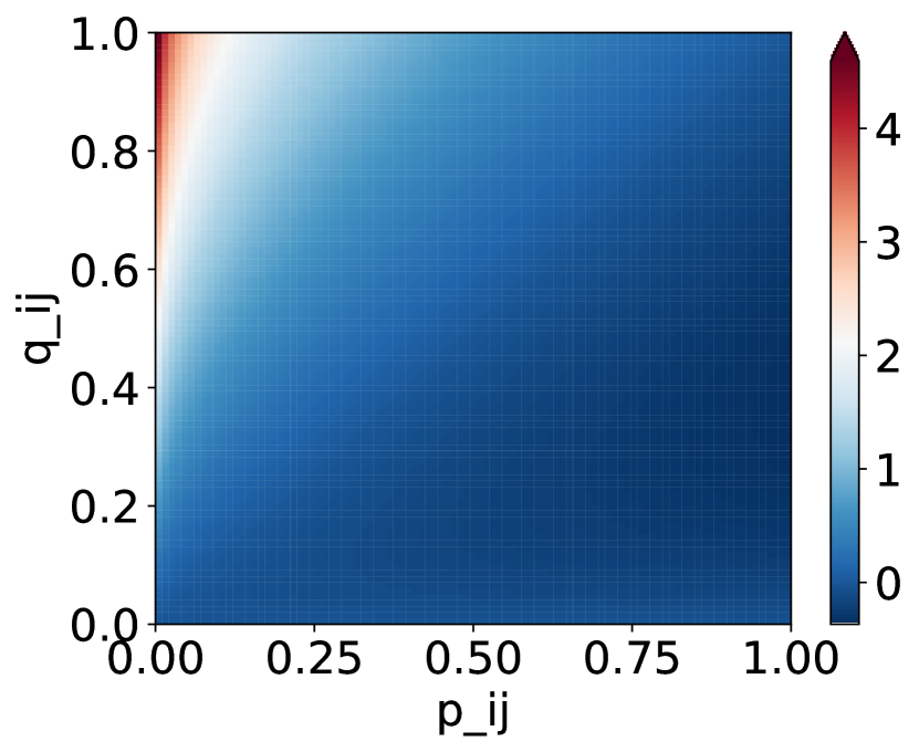
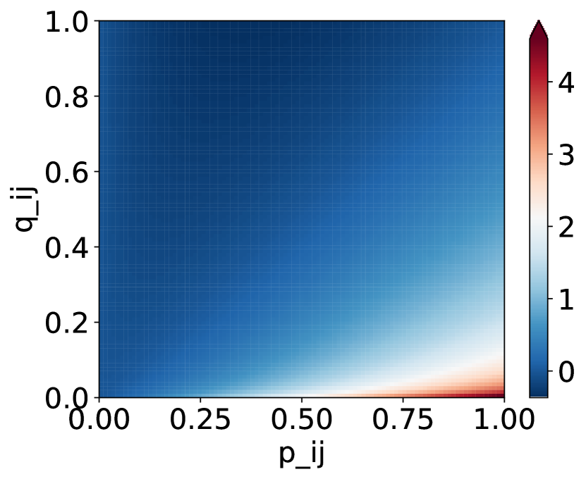
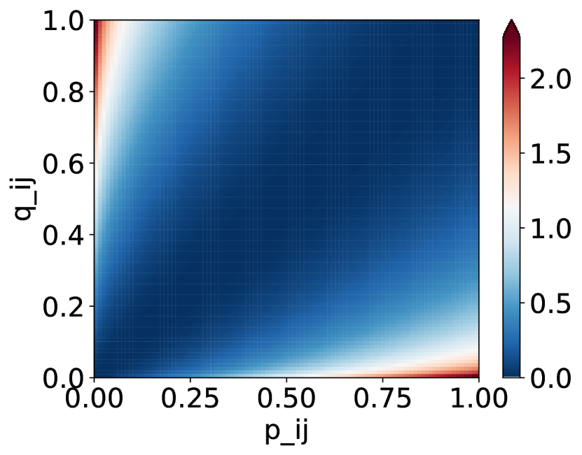
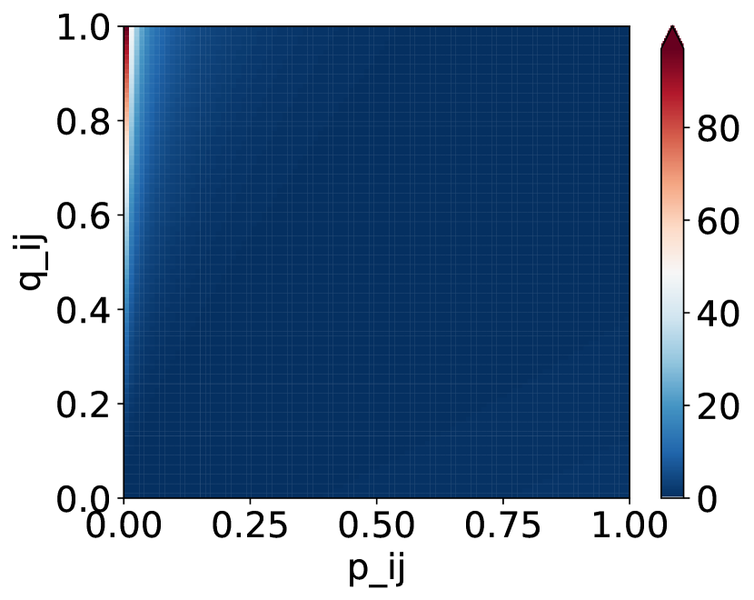
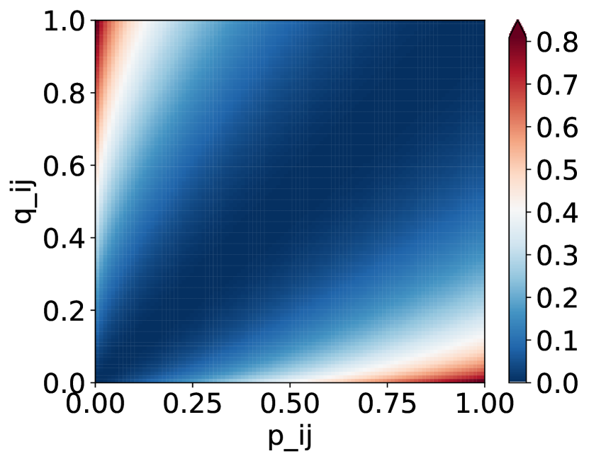
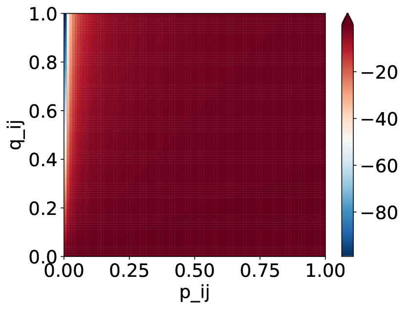
(a) KL

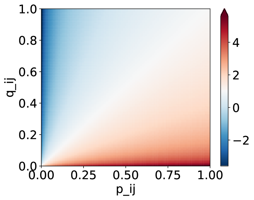
(b) RKL

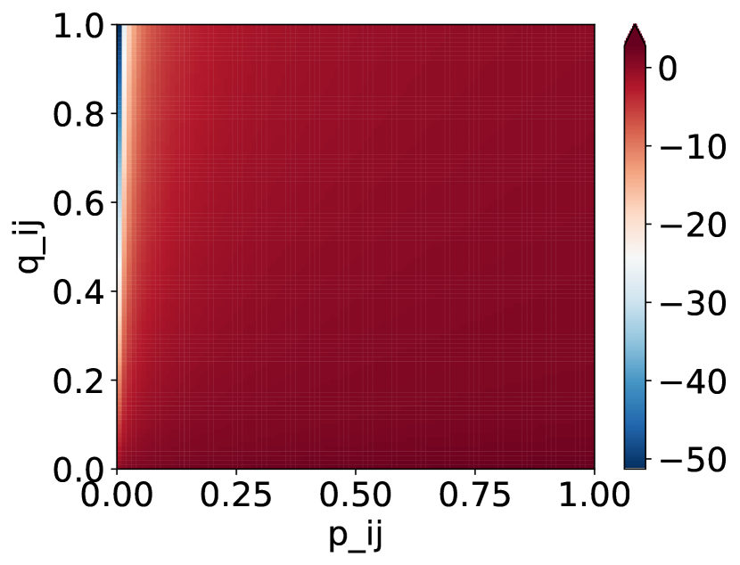
(c) JS

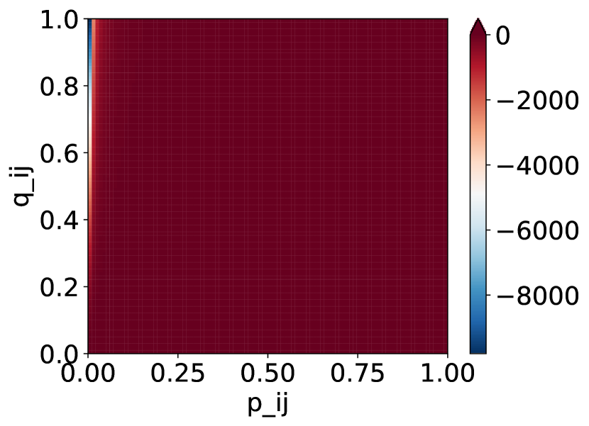
(d) CH

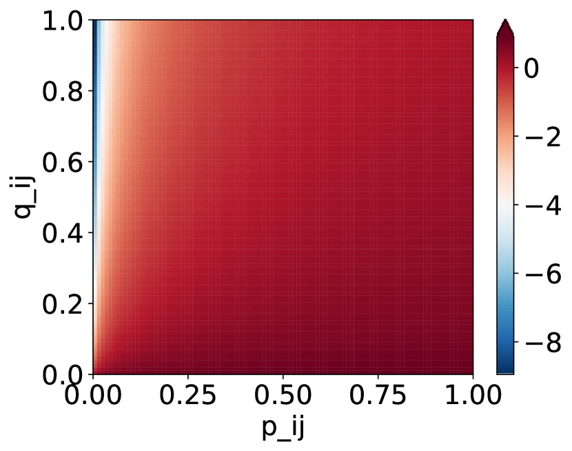
(e) HL

Figure 1: Top: $f$-divergence loss. Bottom: gradient of $f$-divergence. The color limit represents the magnitude of $f$-divergence (resp. gradient of $f$-divergence) of $p_{ij}$ and $q_{ij}$.

3 $f$-Divergence-based Stochastic Neighbor Embedding

KL-divergence is a special case of a broader class of divergences called $f$-divergences. A few popular special cases of $f$-divergences include the reverse KL divergence, Jenson-Shannon divergence, Hellinger distance (HL), total variation distance and $\chi^{2}$-divergence. Of course, each instantiation compares discrepancy between the distributions differently [16] and it would be instructive to study what effects, if any, do these other divergences have on low-D visualizations of a given input. Formally $f$-divergence between two distributions $P$ and $Q$ (over the same measurable space $\Omega$) is defined as

$$D_{f}(P||Q):=\int_{\Omega}f\left(\frac{P(x)}{Q(x)}\right)dQ(x),$$

where $f$ is a convex function such that $f(1)=0$. Intuitively, $f$-divergence tells us the average odds-ratio between $P$ and $Q$ weighted by the function $f$. For the $t$-SNE objective, the generic form of $f$-divergence simplifies to

$$J_{f}(y_{1},\ldots,y_{m}):=D_{f}(P||Q)=\sum_{i\neq j}q_{ij}f\left(\frac{p_{ij}}{q_{ij}}\right).$$ (1)

Table 1 shows a list of common instantiations of $f$-divergences and their corresponding $t$-SNE objectives, which we shall call $ft$-SNE.

Obviously, one expects different optimization objectives (i.e. different choices of $f$) to produce different results. A more significant question is whether these differences have any significant qualitative effects on types of structure discovery.

An indication towards why the choice of $f$ might affect the type of structure revealed is to notice that $f$-divergences are typically asymmetric, and penalize the ratio $p_{ij}/q_{ij}$ (cf. Eq. 1) differently. KL-SNE (i.e. $f$ taken as KL-divergence, cf. Table 1) for instance penalizes pairs of nearby points in the original space getting mapped far away in the embedded space more heavily than faraway points being mapped nearby (since the corresponding $p_{ij}\gg q_{ij}\approx 0$). Thus KL-SNE optimization prefers visualizations that don’t distort local neighborhoods. In contrast, SNE with the reverse-KL-divergence criterion, RKL-SNE, as the name suggests, emphasizes the opposite, and better captures global structure in the corresponding visualizations.

A nice balance between the two extremes is achieved by the JS- and HL-SNE (cf. Table 1), where JS is simply an arithmetic mean of the KL and RKL penalties, and HL is a sort of aggregated geometric mean. Meanwhile, CH-SNE can be viewed as relative version of the (squared) $L_{2}$ distance between the distributions, and is a popular choice for comparing bag-of-words models [23].

We can empirically observe how $p$ and $q$ similarities are penalized by divergence (see Figure 1). Our observation matches with our intuition: KL and CH are sensitive to high $p$ and low $q$, whereas RKL is sensitive to low $p$ and high $q$, and JS and HL are symmetric. The corresponding gradients w.r.t. $q$ show that all divergence are generally sensitive to when $p$ is high and $q$ is low. However, RKL, JS, and HL provide much smoother gradient signals over $p>q$ space. KL penalize strictly towards high $p$ and low $q$ and CH is much stricter towards $p\gg q$ space.

A Neighborhood-level Precision-Recall Analysis. The optimization criterion of $ft$-SNE is a complex non-convex function that is not conducive to a straightforward analysis without simplifying assumptions. To simplify the analysis, we consider pairs of points in a binary neighborhood setting, where, for each datapoint, other datapoints are either in its neighborhood, or not in its neighborhood.

Let $N_{\epsilon}(x_{i})$ and $N_{\epsilon}(y_{i})$ denote the neighbors of points $x_{i}$ and $y_{i}$ by thesholding the pairwise similarities $p_{j|i}$ and $q_{j|i}$ at a fixed threshold $\epsilon$, respectively. Let $r_{i}:=|N_{\epsilon}(x_{i})|$ and $k_{i}:=|N_{\epsilon}(y_{i})|$ denote the number of true and retrieved neighbors. Our simplifying binary neighborhood assumption can be formalized as:

$$\begin{aligned} p_{ij}&:=\begin{cases}a_{i},&x_{j}\in N_{\epsilon}(x_{i})\\ b_{i},&x_{j}\notin N_{\epsilon}(x_{i})\end{cases},\end{aligned}\begin{aligned} q_{ij}&:=\begin{cases}c_{i},&y_{j}\in N_{\epsilon}(y_{i})\\ d_{i},&y_{j}\notin N_{\epsilon}(y_{i})\end{cases}.\end{aligned}$$

where $a_{i}$ and $c_{i}$ are large ($a_{i}\geq\frac{1-\delta}{r_{i}}$, $c_{i}\geq\frac{1-\delta}{k_{i}}$) and $b_{i}$ and $d_{i}$ are small ($b_{i}\leq\frac{\delta}{m-r_{i}-1}$, $d_{i}\leq\frac{\delta}{m-k_{i}-1}$), for small $\delta$.

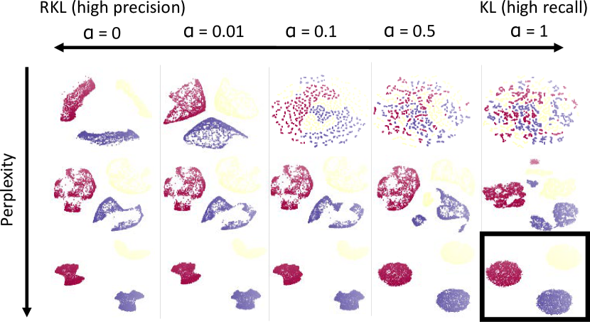
(a) 3 well-separated Gaussian clusters

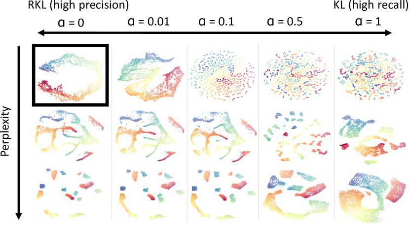
(b) Swiss roll manifold

Figure 2: $ft$-SNE embeddings obtained with interpolated divergences between KL and RKL. The perplexity for each row corresponds to 10, 100, and 500 respectively.

In this binary formulation, we can rewrite each of the $f$-divergences in terms related to the embedding precision, the fraction of embedding-neighbors are true neighbors, and the recall, the fraction of true neighbors are also embedding-neighbors. Define $n_{\operatorname{{\textrm{TP}}}}^{i}:=|N_{\epsilon}(x_{i})\cap N_{\epsilon}(y_{i})|$, $n_{\textrm{FP}}^{i}:=|N_{\epsilon}(y_{i})\setminus N_{\epsilon}(x_{i})|$ and $n_{\textrm{FN}}^{i}:=|N_{\epsilon}(x_{i})\setminus N_{\epsilon}(y_{i})|$ to denote the number of true-positive, false-positive and false-negative neighbors respectively. In this notation, per-neighborhood precision is $n_{\operatorname{{\textrm{TP}}}}^{i}/k_{i}=1-n_{\operatorname{{\textrm{FP}}}}^{i}/k_{i}$ and recall is $n_{\operatorname{{\textrm{TP}}}}^{i}/r_{i}=1-n_{\operatorname{{\textrm{FN}}}}^{i}/r_{i}$. This information retrieval analysis has previously been performed for KL-SNE [20]. Novelly, we extend it to other $f$-divergences to understand their assumptions.

Proposition 1.

Under the binary-neighborhood assumption, for $\delta$ sufficiently small,

1. $J_{\operatorname{{\textrm{KL}}}}\propto\Big{(}\sum_{i}\underbrace{{n^{i}_{\operatorname{{\textrm{FN}}}}}/{r_{i}}}_{1-\textrm{recall}}\Big{)}$, maximizes recall.

2. $J_{\operatorname{{\textrm{RKL}}}}\propto\Big{(}\sum_{i}\underbrace{{n^{i}_{\operatorname{{\textrm{FP}}}}}/{k_{i}}}_{1-\textrm{precision}}\Big{)}$ maximizes precision.

3. $J_{\operatorname{{\textrm{JS}}}}\propto J_{\operatorname{{\textrm{KL}}}}+J_{\operatorname{{\textrm{RKL}}}}$ balances precision and recall,

4. The first two terms of HL-SNE balance precision and recall (the coefficients are close to 1, since $\delta$ is small). The last term forces preservation of neighborhood sizes, and strongly penalizes small embedding neighborhoods when precision is high.

   $$J_{\operatorname{{\textrm{HL}}}}\propto\sum_{i} \Big{[}\underbrace{\Big{(}\frac{n_{\operatorname{{\textrm{FN}}}}^{i}}{r_{i}}\Big{)}}_{1-\textrm{recall}}\cdot(1-O({(\delta r_{i})}^{\frac{1}{2}}))\Big{]}+\Big{[}\underbrace{\Big{(}\frac{n_{\operatorname{{\textrm{FP}}}}^{i}}{k_{i}}\Big{)}}_{1-\textrm{precision}}\cdot(1-O({(\delta k_{i})}^{\frac{1}{2}}))\Big{]}+\underbrace{\Big{(}\frac{n_{\operatorname{{\textrm{TP}}}}^{i}}{k_{i}}\Big{)}}_{\textrm{precision}}\cdot\underbrace{\Big{(}\sqrt{\frac{r_{i}}{k_{i}}}-1\Big{)}^{2}}_{\begin{subarray}{c}\textrm{neighborhood}\\ \textrm{size ratio}\end{subarray}}.$$

5. CH-SNE is biased towards maximizing recall, since the multiplier of recall is much larger than that on precision. Like HL-SNE, the last term forces preservation of neighborhood sizes, and strongly penalizes small embedding neighborhoods when precision is high.

   $$J_{\operatorname{{\textrm{CH}}}}\propto\sum_{i} \Big{[}\underbrace{\Big{(}\frac{n_{\operatorname{{\textrm{FN}}}}^{i}}{r_{i}}\Big{)}}_{1-\textrm{recall}}\cdot\Big{(}\frac{m-k_{i}}{r_{i}\delta}\Big{)}\Big{]}+\underbrace{\Big{(}\frac{n_{\operatorname{{\textrm{FP}}}}^{i}}{k_{i}}\Big{)}}_{1-\textrm{precision}}+\Big{[}\underbrace{\Big{(}\frac{n_{\operatorname{{\textrm{TP}}}}^{i}}{k_{i}}\Big{)}}_{\textrm{precision}}\cdot\underbrace{\Big{(}{\frac{r_{i}}{k_{i}}}-1\Big{)}^{2}}_{\begin{subarray}{c}\textrm{neighborhood}\\ \textrm{size ratio}\end{subarray}}\Big{]}.$$

This proposition corroborates our intuition (see also Table 1), and provides a relationship between the proposed $ft$-SNE criteria and the types of neighborhood similarities that are preserved. KL-SNE maximizes neighborhood recall, while RKL-SNE maximizes neighborhood precision. All other criteria balance precision and recall in different ways. JS-SNE provides equal weight to precision and recall. HL-SNE gives approximately equal weight to precision and recall, with an extra term encouraging the original and embedding neighborhood sizes to match. This regularization term gives more severe penalties if the embedding neighborhood is much smaller than the original neighborhood than the reverse, and thus HL-SNE can be viewed as a regularized version of JS-SNE. CH-SNE gives more weight to maximizing recall, again with an extra term encouraging the original and embedding neighborhood sizes to match, and is and thus similar to a regularized version of KL-SNE.

Next, we connect these precision-recall interpretations of the various criteria to the types of intrinsic structure they preserve. Suppose the intrinsic structure within the data is clusters. A good embedding of this data would have points belonging to the same true cluster all grouped together in the visualization, but the specific locations of the embedded points within the cluster do not matter. Thus, cluster discovery requires good neighborhood recall, and one might expect KL-SNE to perform well. For neighborhood sizes similar to true cluster sizes, this argument is corroborated both theoretically by previous work [12, 3] and empirically by our experiments (Experiments Section). Both theoretically and practically, the perplexity parameter—which is a proxy for neighborhood size—needs to be set so that the effective neighborhood size matches the cluster size for successful cluster discovery.

If the intrinsic structure within the data is a continuous manifold, a good embedding would preserve the smoothly varying structure, and not introduce artificial breaks in the data that lead to the appearance of clusters. Having a large neighborhood size (i.e. large perplexity) may not be conducive to this goal, again because the SNE optimization criterion does not care about the specific mapped locations of the datapoints within the neighborhood. Instead, it is more preferable to have small enough neighborhood where the manifold sections are approximately linear one require high precision in these small neighborhoods. Thus one might expect RKL-SNE to fare well manifold discovery tasks. Indeed, this is also corroborated practically in our experiments. (To best of our knowledge, no theory work exists on this.)

Table 2: Variational $ft$-SNE.

$D_{f}(P\|Q)$	$f(t)$	$f^{*}(t)$	$h(x)$
Kullback-Leibler (KL)	$t\log t$	$\exp(t-1)$	$x$
Reverse-KL (RKL)	$-\log t$	$-1-\log(-t)$	$-\exp(-x)$
Jensen-Shannon (JS)	$-(t+1)\log\frac{(1+t)}{2}+t\log t$	$-\log(1-\exp(t))$	$\log(2)-\log\left(1+\exp(-x)\right)$
Hellinger distance (HL)	$(\sqrt{t}-1)^{2}$	$\frac{t}{1-t}$	$1-\exp(-x)$
Chi-square ($\mathcal{X}^{2}$ or CS)	$(t-1)^{2}$	$\frac{1}{4}t^{2}+t$	$x$

Variational $ft$-SNE for practical usage and improved optimization. The $ft$-SNE criteria can be optimized using gradient descent or one of its variants, e.g. stochastic gradient descent, and KL-SNE is classically optimized in this way. The proposed $ft$-SNE criteria (including KL-SNE) are non-convex, and gradient descent may not converge to a good solution. We explored minimizing the $ft$-SNE criteria by expressing it in terms of its conjugate dual [17, 16]:

$$D_{f}(P||Q)=\sum_{i\neq j}\left[q_{ij}\left(\sup_{h\in\mathcal{H}}h((x_{i},x_{j}))\frac{p_{ij}}{q_{ij}}-f^{*}(h((x_{i},x_{j})))\right)\right]$$

where $\mathcal{H}$ is the space of real-valued functions on the underlying measure space and $f^{*}$ is the Fenchel conjugate of $f$. In this equation, the maximum operator acts per data point, making optimization infeasible. Instead, we optimize the variational lower bound

$$D_{f}(P||Q)\geq\sup_{h\in\mathcal{H}}\sum_{i\neq j}\left[h((x_{i},x_{j}))p_{ij}-f^{*}(h((x_{i},x_{j})))q_{ij}\right],$$

which is tight for sufficiently expressive $\mathcal{H}$. In practice, one uses a parameteric hypothesis class $\bar{\mathcal{H}}$, and we use multilayer, fully-connected neural networks. Table 2 shows a list of common instantiations of $f$-divergences and their corresponding $h(x)$ functions. Our variational form of $ft$-SNE objective (or $vft$-SNE) finally becomes the following minimax problem

$$J( y_{1},\ldots,y_{m})=\min_{y_{1},\ldots,y_{m}}\max_{\bar{h}\in\bar{\mathcal{H}}}\sum_{i\neq j}\left[\bar{h}((x_{i},x_{j}))p_{ij}-f^{*}\left(\bar{h}((x_{i},x_{j}))\right)q_{ij}\right].$$

We alternatively optimize $y_{1},\ldots,y_{m}$ and $\bar{h}$ (see Algorithm 1, more details available in S.M.).

Algorithm 1 Variational (Adversarial) SNE Optimization Algorithm

1:procedure Optimization(Dataset $\{X_{tr},X_{vl}\}$, learning rate $\eta$, $f$-divergence $J$)

2:     Initialize the discriminant parameter $\phi$.

3:     while $\phi$ has not converged do

4:         for $j=1,\ldots,J$ do

5:              $\phi_{t+1}=\phi_{t}+\eta\nabla_{\phi}J$.          

6:         for $k=1,\ldots,K$ do

7:              $y^{i}_{t+1}=y^{i}_{t}-\eta_{y}\nabla_{y}J$.               

Table 3: Best $ft$-SNE method for each dataset and criterion, according to maximum F-score in Figure 3 and 7.

		Data-Embeddings			Class-Embedings
Data	Type	K-Nearest	K-Farthest	F-Score on X-Y	F-Score on Z-Y
MNIST (Digit 1)	Manifold	RKL	RKL	RKL	-
Face	Manifold	HL,RKL	RKL	RKL	JS
MNIST	Clustering	KL	KL	CS	KL
GENE	Clustering	KL	KL	KL	KL
20 News Groups	Sparse &	CS	CS	CS	HL
	Hierachical
ImageNet (sbow)	Sparse &	CS	CS	CS	KL
	Hierachical

4 Experiments

In this section, we compare the performance of the proposed $ft$-SNE methods in preserving different types of structure present in selected data sets. Next, we compare the efficacy of optimizing the primal versus the dual form of the $ft$-SNE. Details about the datasets, optimization parameters, and architectures are described in the Supplementary Material (S.M.).

Datasets. We compared the proposed $ft$-SNE methods on a variety of datasets with different latent structures. The MNIST dataset consists of images of handwritten digits from 0 to 9 [10], thus the latent structure is clusters corresponding to each digit. We also tested on just MNIST images of the digit 1, which corresponds to a continuous manifold. The Face dataset, proposed in [18], consists of rendered images of faces along a 3-dimensional manifold corresponding to up-down rotation, left-right rotation, and left-right position of the light source. The Gene dataset consists of RNA-Seq gene expression levels for patients with five different types of tumors [21], and thus has a cluster latent structure. The 20-Newsgroups dataset consisted of text articles from a hierarchy of topics [9], and thus the latent structure corresponded to a hierarchical clustering. In addition, we used a bag-of-words representation of the articles, thus the feature representation is sparse (many of the features in the original representation will be 0). We also examined two synthetic datasets: the Swiss Roll dataset [18] which has a continuous manifold latent structure, and a simple dataset consisting of 3 Gaussian clusters in 2 dimensions, which has a cluster latent structure. Details of these datasets can be found in Appendix.

4.1 Comparison of $f$-divergences for SNE

We developed several criteria for quantifying the performance of the different $ft$-SNE methods. Our criteria are based on the observation that, if the local structure is well-preserved, then the nearest neighbours in the original data space $\mathcal{X}$ should match the nearest neighbours in the embedded space $\mathcal{Y}$. In addition, many of our datasets include a known latent variable, e.g. the discrete digit label for MNIST and the continuous head angle for Face. Thus, we also measure how well the embedded space captures the known structure of the latent space $\mathcal{Z}$. We define the neighbors $N_{\epsilon}(x_{i})$, $N_{\epsilon}(y_{i})$, and $N_{\epsilon}(z_{i})$ of points $x_{i}$, $y_{i}$, and $z_{i}$ by thresholding the pairwise similarity $p_{j|i}$, $q_{j|i}$ and $r_{j|i}$, respectively, at a selected threshold $\epsilon$. Here, $r_{j|i}=r(z_{j}|z_{i})$ is the pairwise similarity in the latent space $\mathcal{Z}$. For discrete labels, we define $r_{j|i}\propto\mathbb{I}(z_{i}=z_{j})$. For continuous latent spaces, we use a t-distribution.

Using these definitions of neighbors, we can define precision and recall, considering the original $\mathcal{X}$ or latent $\mathcal{Z}$ spaces as true and the embedded space $\mathcal{Y}$ as the predicted:

$$\allowdisplaybreaks\text{Precision}_{X}(\epsilon) =\frac{1}{N}\sum^{N}_{i}\frac{|N_{\epsilon}(y_{i})\cap N_{\epsilon}(x_{i})|}{|N_{\epsilon}(y_{i})|},\quad \text{Precision}_{Z}(\epsilon)=\frac{1}{N}\sum^{N}_{i}\frac{|N_{\epsilon}(y_{i})\cap N_{\epsilon}(z_{i})|}{|N_{\epsilon}(y_{i})|}$$

$$\text{Recall}_{X}(\epsilon) =\frac{1}{N}\sum^{N}_{i}\frac{|N_{\epsilon}(y_{i})\cap N_{\epsilon}(x_{i})|}{|N_{\epsilon}(x_{i})|},\quad \text{Recall}_{Z}(\epsilon)=\frac{1}{N}\sum^{N}_{i}\frac{|N_{\epsilon}(y_{i})\cap N_{\epsilon}(z_{i})|}{|N_{\epsilon}(z_{i})|}.$$

Alternatively, we can measure how well the embedded space preserves the nearest and farthest neighbor structure. Let $NN_{K}(x_{i})$ and $NN_{K}(y_{i})$ indicate the $K$ nearest neighbors and $FN_{K}(x_{i})$ and $FN_{K}(y_{i})$ indicate the $K$ farthest neighbors. We define

$$\text{NN-Precision}(K) =\frac{1}{NK}\sum^{N}_{i}|\text{NN}_{K}(y_{i})\cap\text{NN}_{K}(x_{i})|,$$

$$\text{FN-Precision}(K) =\frac{1}{NK}\sum^{N}_{i}|\text{FN}_{K}(y_{i})\cap\text{FN}_{K}(X_{i})|$$

For each of the datasets, we produced Precision${}_{X}(\epsilon)$-Recall${}_{X}(\epsilon)$ and Precision${}_{Z}(\epsilon)$-Recall${}_{Z}(\epsilon)$ curves by varying $\epsilon$, and $\text{NN Precision}(K)$-$\text{FN Precision}(K)$ curves by varying $K$. Results are shown in Figure 3 and 7. Table 5-12 summarizes these results by presenting the algorithm with the highest maximum f-score per criterion. For the two manifold datasets, MNIST-Digit-1 and Face, RKL and JS outperformed KL. This reflects the analysis (see Proposition 1) that RKL and JS emphasize global structure more than KL, and global structure preservation is more important for manifolds. Conversely, KL performs best on the two cluster datasets, MNIST and GENE. Finally, CH and HL performed best on the hierarchical dataset, News (cf. 23).

MNIST1

Face

MNIST

GENE

NEWS

SBOW

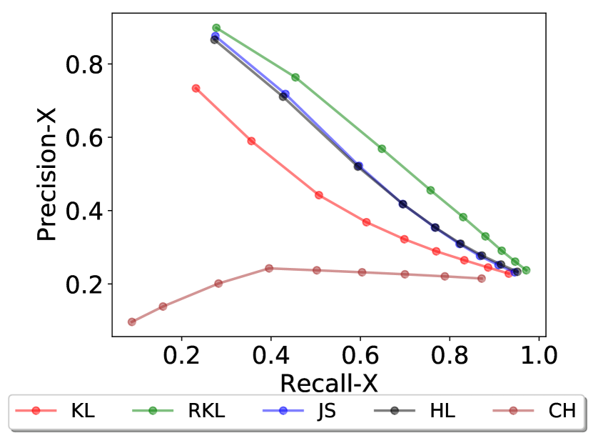
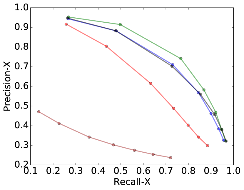
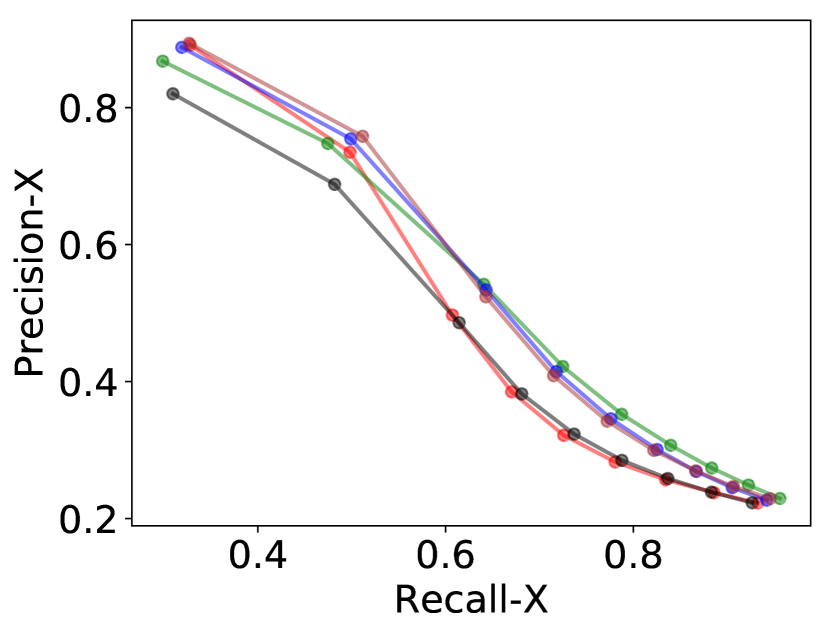
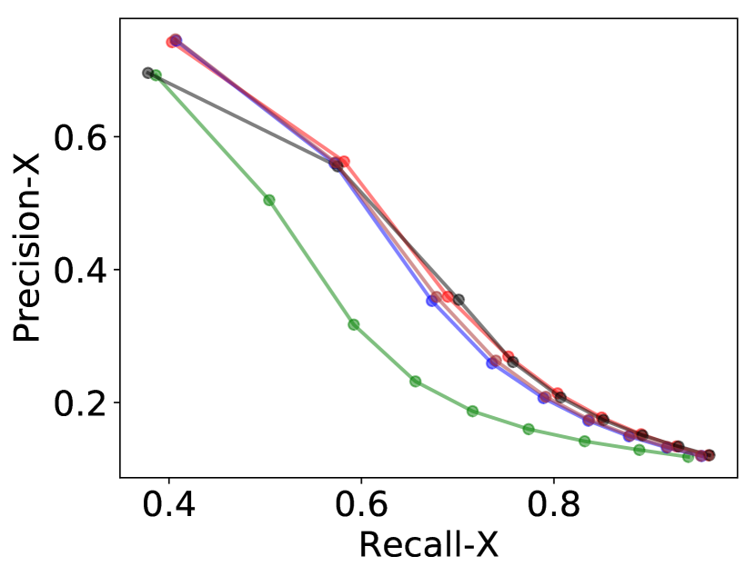
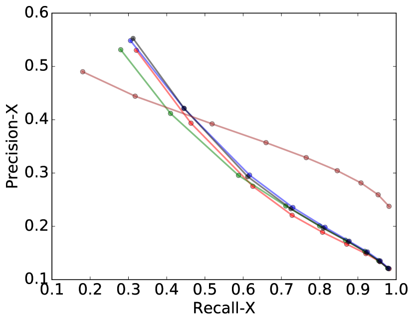
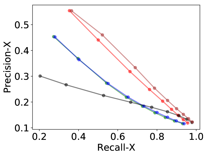
(a) Precision-Recall curve for XY ($\text{Precision}_{X}(\epsilon)$ vs. $\text{Recall}_{X}(\epsilon)$)

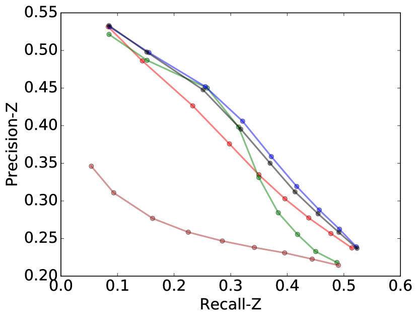
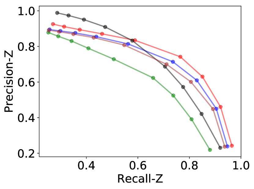
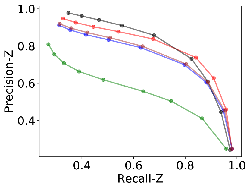
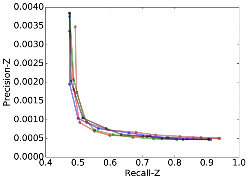
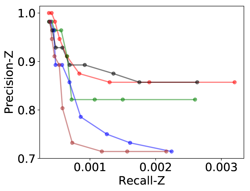
(b) Precision-Recall curve for ZY ($\text{Precision}_{Z}(\epsilon)$ vs. $\text{Recall}_{Z}(\epsilon)$)

Figure 3: Precision-Recall curves for each of the proposed algorithms on all datasets. Each row corresponds to different quantitative criteria, each column to a different dataset, and each line to a different algorithm.

To better understand the relative strengths of KL and RKL, we qualitatively compared the embeddings resulting from interpolating between them:

$$\alpha KL\text{-SNE}+(1-\alpha)RKL\text{-SNE}$$ (2)

for $\alpha=0,0.05,0.1,0.5,1.0$ ($\alpha=.5$ corresponds to JS). Figure 2 presents the embedding results for two synthetic datasets: the Swiss Roll which is a continuous manifold, and three Gaussian clusters, for a range of perplexity and $\alpha$ values. We observe that RKL worked better for manifolds with low perplexity while KL worked better clusters with larger perplexity (as predicted in Section 3. In addition, KL broke up the continuous Swiss Roll manifold into disjoint pieces, which produces smoother embeddings compare to KL-SNE under low perplexity. Finally, we did not see a continuous gradient in embedding results as we changed $\alpha$. Instead, even for $\alpha=0.1$, the Swiss Roll embedding was more similar to the discontinuous KL embedding. For this dataset, the embedding produced by JS was more similar to that produced by KL than RKL. For the three Gaussian dataset, all algorithms separated the three clusters, however KL and JS correctly formed circular clusters, while smaller values of $\alpha$ resulted in differently shaped clusters.

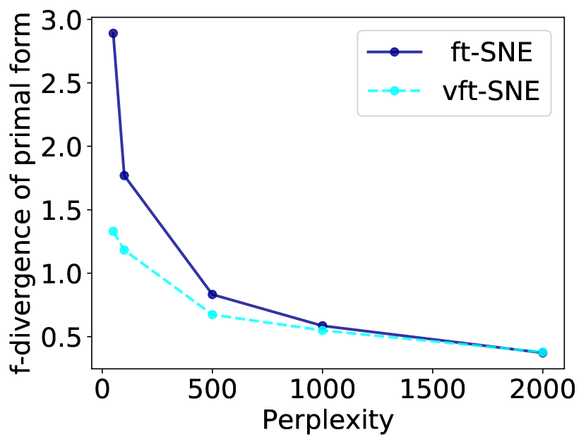
(a) KL

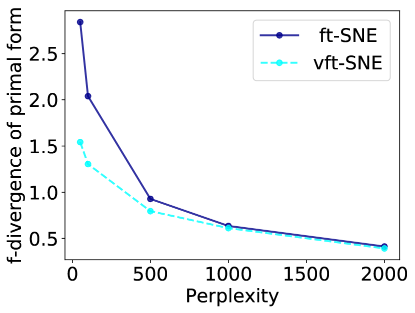
(b) JS

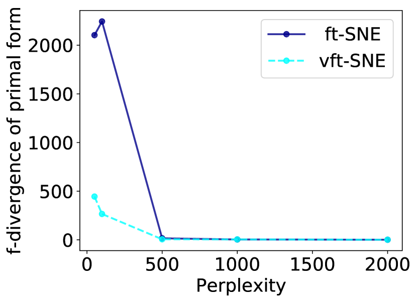
(c) CH

Figure 4: Log of the primal $ft$-SNE loss for the $ft$-SNE and $vft$-SNE algorithms for different perplexities on MNIST. The number of updates were set to J:K=10:10 and two hidden layer (10-20) deep ReLU neural network.

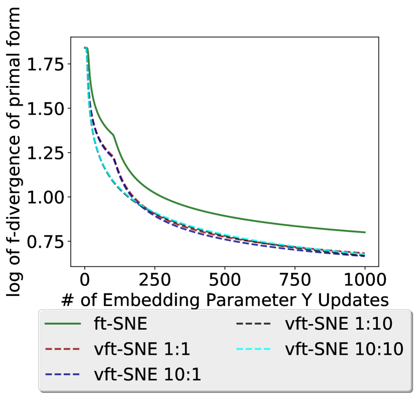
(a) Number of updates ($J$:$K$)

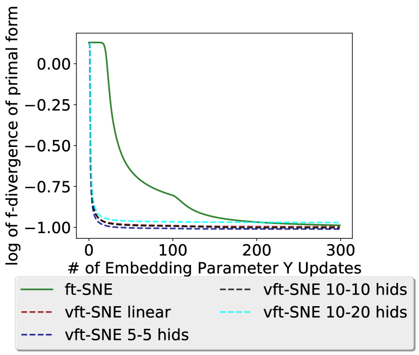
(b) Network depth

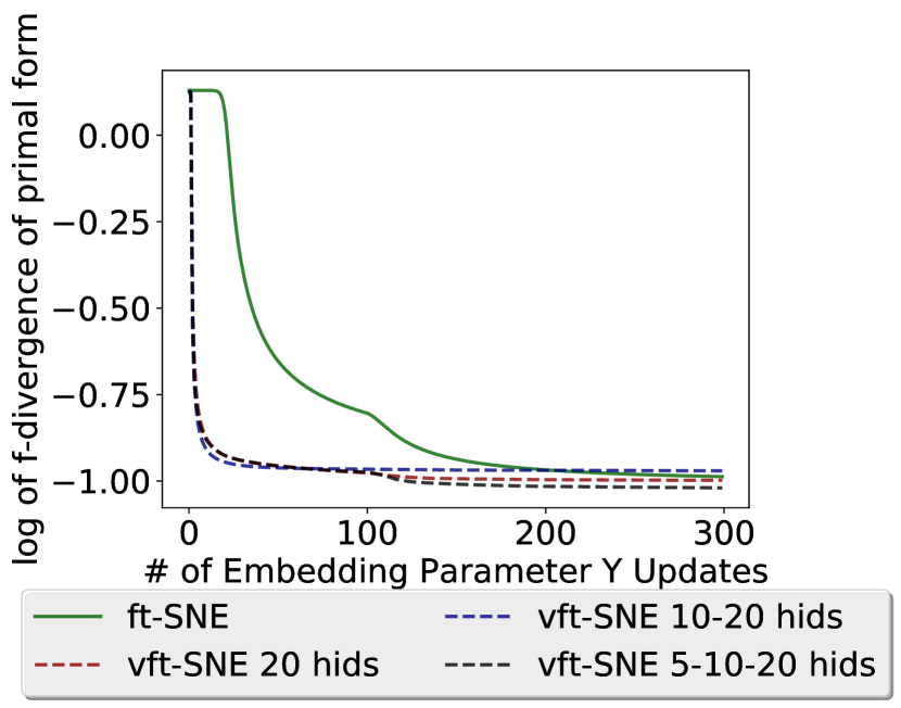
(c) Network width

Figure 5: Comparison of log $t$-SNE criterion for different parameter choices. All plots show results for the KL divergence on the MNIST dataset (perplexity 2,000), results for other divergences and datasets are in S.M. (a) Different numbers of updates to the discriminator and embedding weights with fixed network architecture (2 layers of 10 and 20 hidden units). (b) Different network widths, with fixed $J$:$K$ = 10:10. (c) Different network depths (widths specified in legend), $J$:$K$ = 10:10.

4.2 Optimization of the primal vs. variational forms

In this section, we quantitatively and qualitatively compared the efficacy of optimizing the primal, $ft$-SNE, versus the variational, $vft$-SNE, forms of the criteria. Quantitatively, we compared the primal $ft$-SNE criteria at solutions found using both methods during and after optimization.

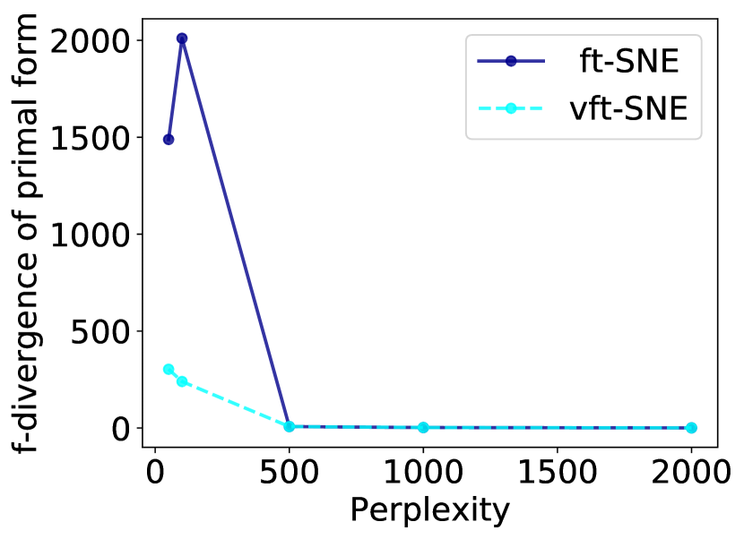
(a) MNIST1

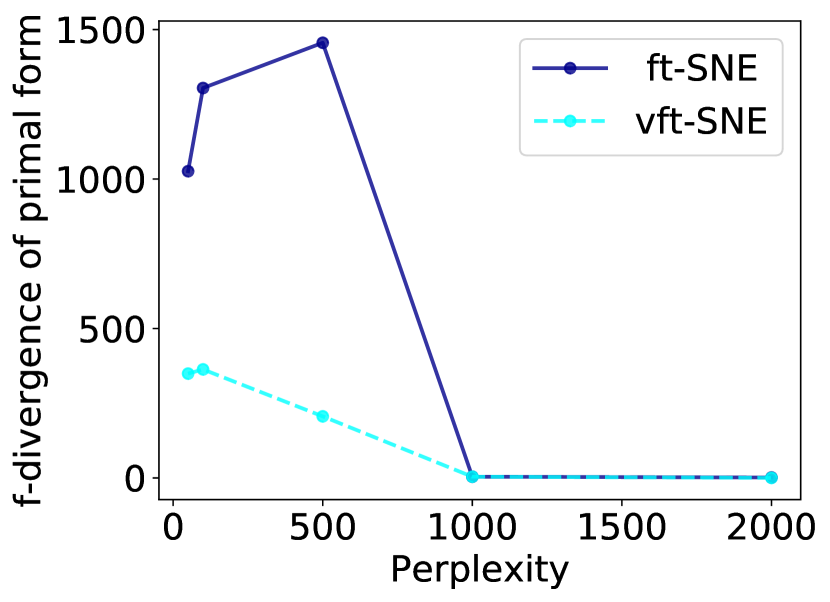
(b) NEWS

(c) Chi-Square

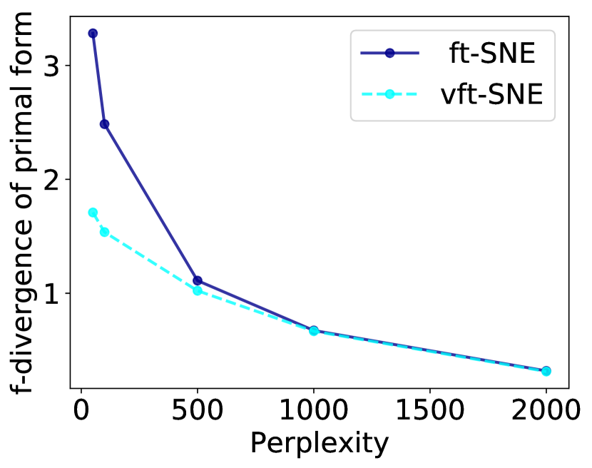
(d) MNIST1

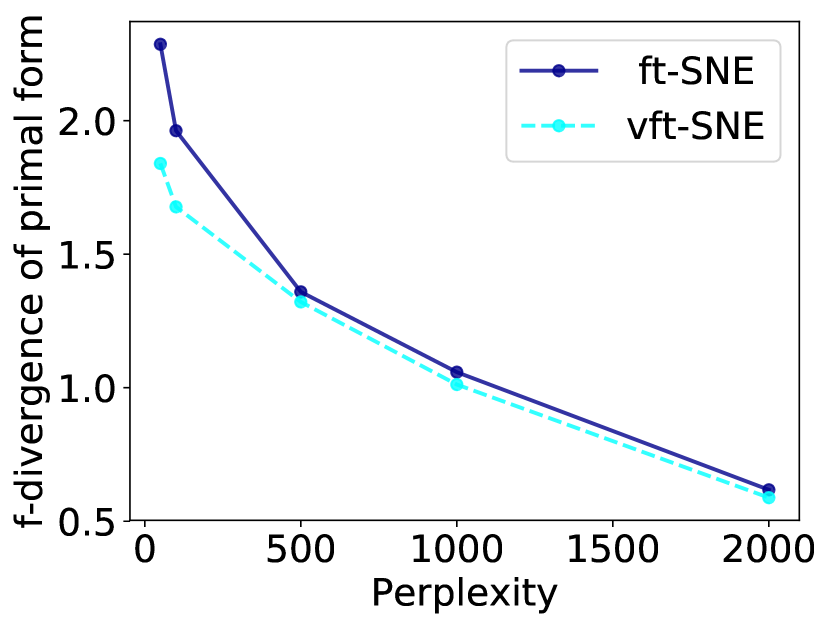
(e) NEWS

(f) Jensen-Shannon

Figure 13: $ft$-SNE and $vft$-SNE Loss with respect to different perplexities MNIST1 and NEWS.

Figure 4 shows the log primal $ft$-SNE criteria of the final solutions using both optimization methods for different $f$-divergences and different perplexities for MNIST (Supp. Fig. 13 shows results for other datasets). We found that for small perplexities $vft$-SNE outperforms $ft$-SNE, while this difference decreases as perplexity increases $ft$-SNE and $vft$-SNE converges to same loss values as the perplexity increases. However, even at perplexity $2000$, $vft$-SNE achieves a slightly lower loss than $ft$-SNE. This is surprising since $vft$-SNE minimizes a lower bound of $ft$-SNE, the criterion we are using for comparison, and suggests that optimizing the primal form using gradient descent can result in bad local minima.

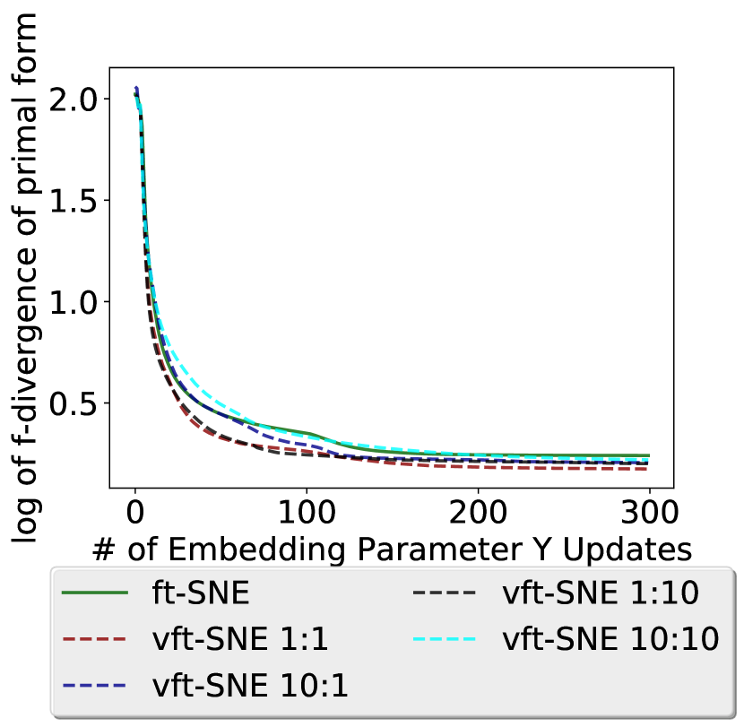
(a) CS-SNE

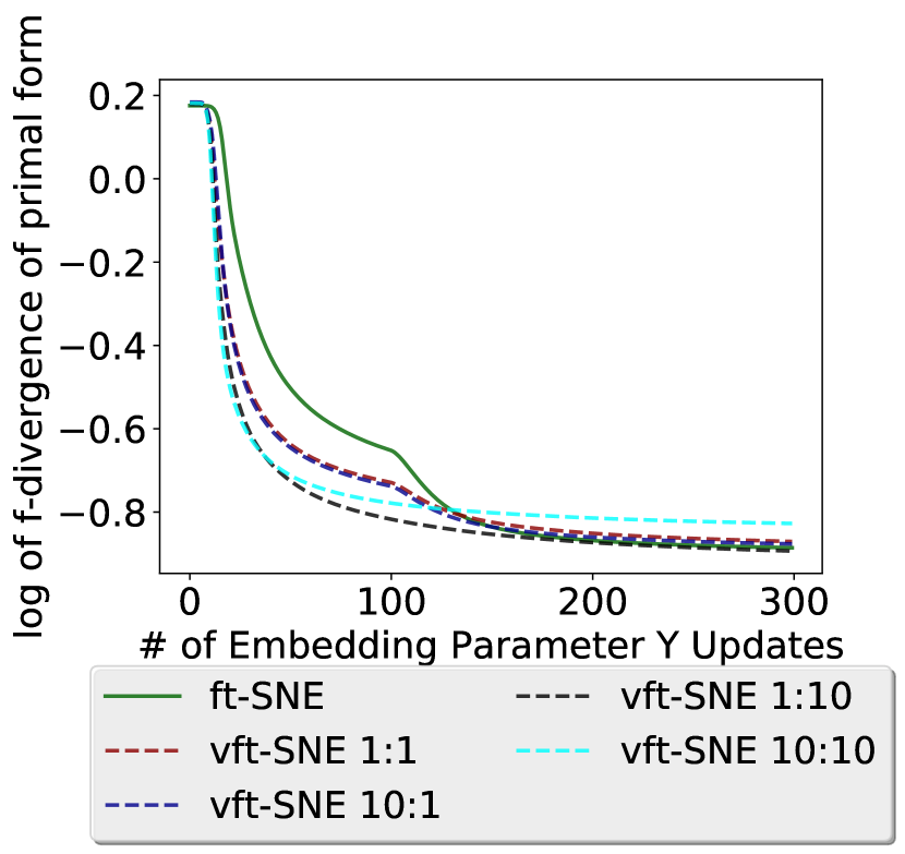
(b) JS-SNE

(c) KL-SNE

(d) MNIST

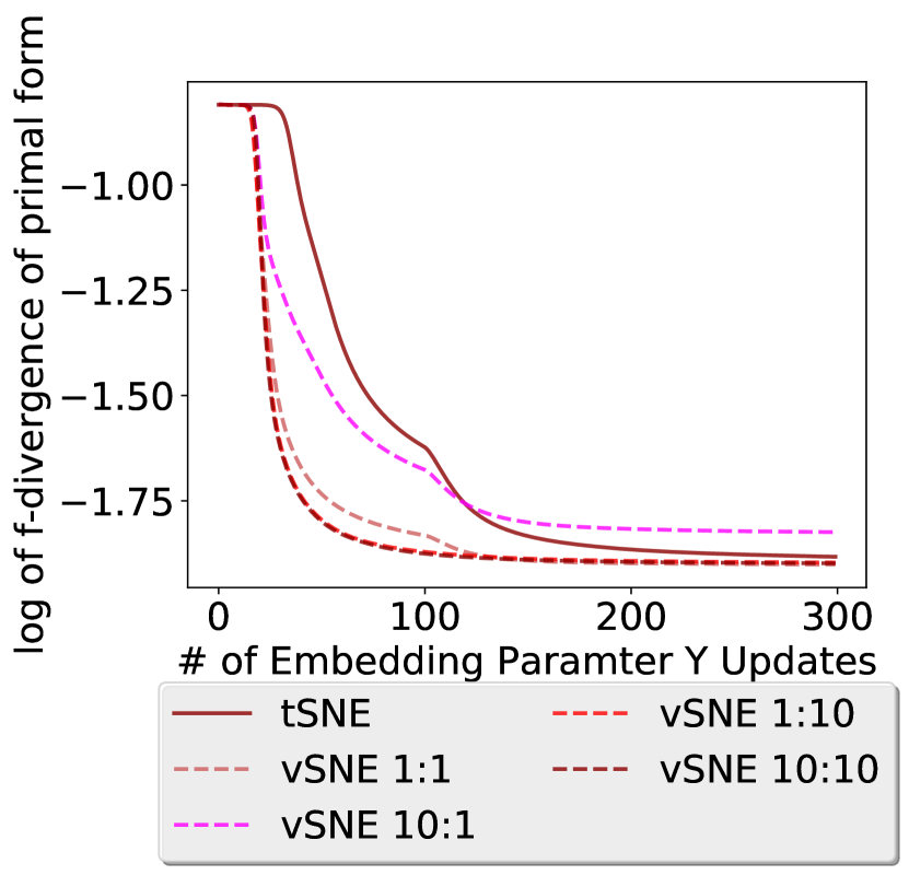
(e) MNIST1

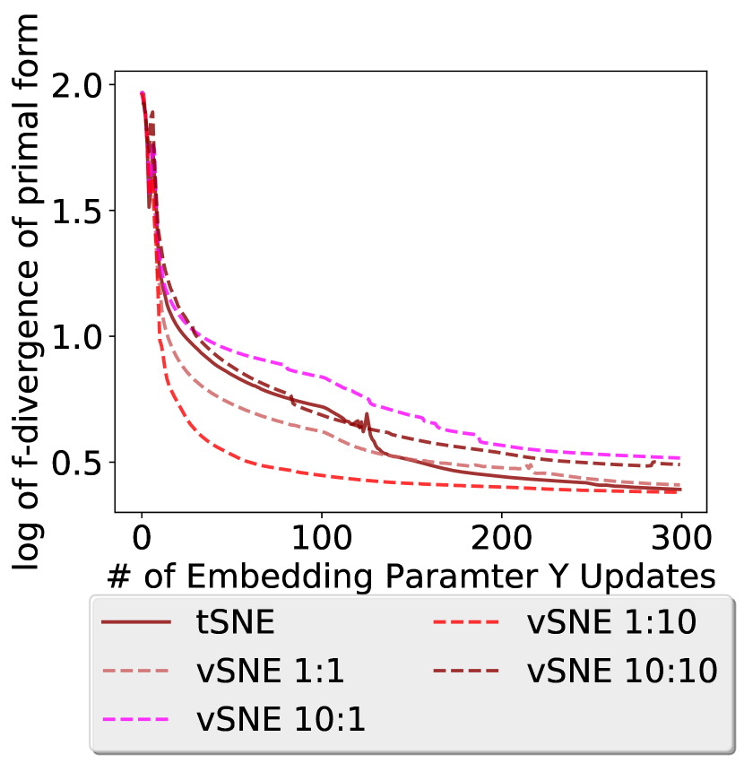
(f) NEWS

(g) Chi-Square

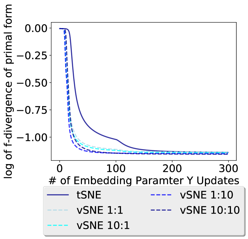
(h) MNIST1

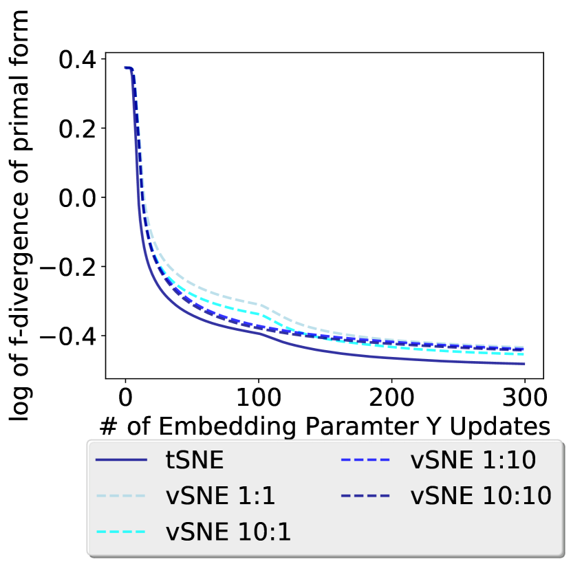
(i) NEWS

(j) Jensen-Shannon

Figure 11: Log $ft$-SNE criterion during optimization for different choices of $J$ and $K$ on MNIST, MNIST1, and NEWS. Two hidden layer (10-20) deep ReLU neural network was used as the discriminator and perplexity was set to 2,000.

We next evaluated the performance of the $vft$-SNE algorithm as we vary some of the parameters of the method. Figure 5a compares the results as we vary the number of updates $J$ and $K$ to perform to the discriminator and embedding weights (Algorithm 1). For the KL divergence, we found that optimizing the variational form performed better for all choices of $J$ and $K$, both in terms of the rate of convergence and the final solution found. For the CH and JS divergences, nearly all choices of $J$ and $K$ resulted in faster optimization (see Supp. Fig. 11). This plot is in terms of the number of updates, wall clock time is shown in Table 13 (S.M.).

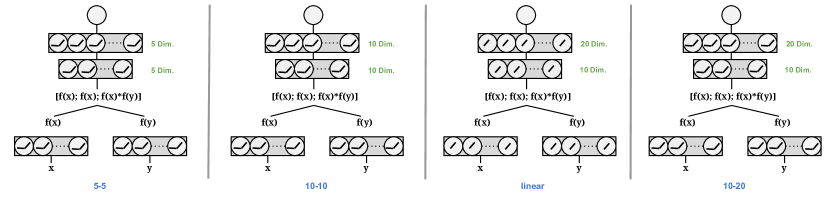
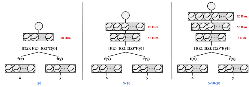
Figure 14: Discriminant Architecture : # of Hidden Layer Size

Figure 15: Discriminant Architecture : # of Hidden Layer Depth

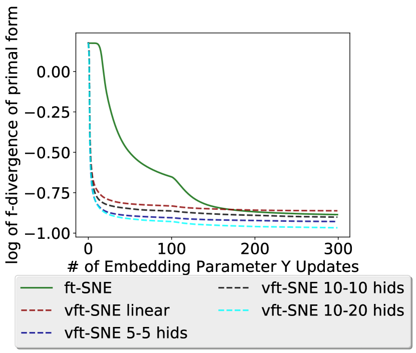
(b) JS-SNE

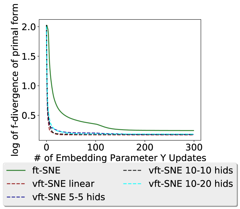
(c) CS-SNE

(d) Varying discriminator network width

(e) KL-SNE

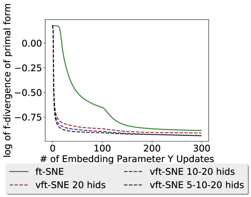
(f) JS-SNE

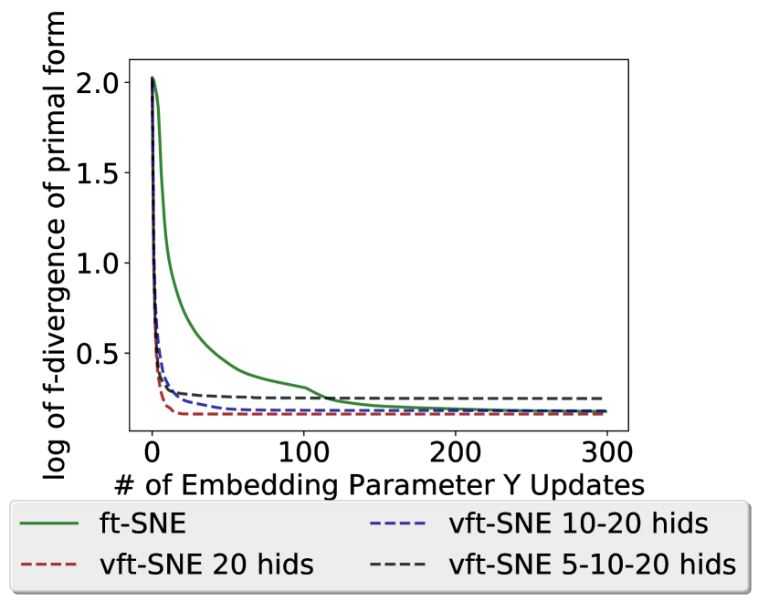
(g) CS-SNE

(h) Varying discrimnator network depth

Figure 16: Log $ft$-SNE criterion during optimization for different discriminator network architectures on MNIST. In (a), we compare two-layer networks of different widths (legend indicates number of units in first and second hidden layers). In (b), we compare networks with different depths (legend indicates number of units in each hidden layer). The number of updates were set to J:K=10:10 and perplexity was set to 2,000.

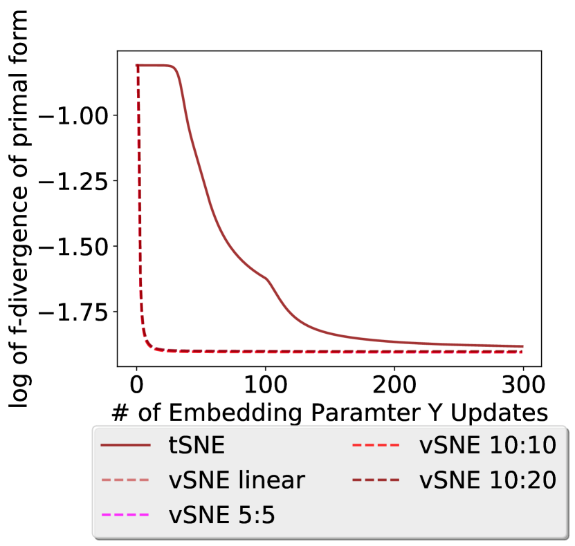
(a) MNIST1

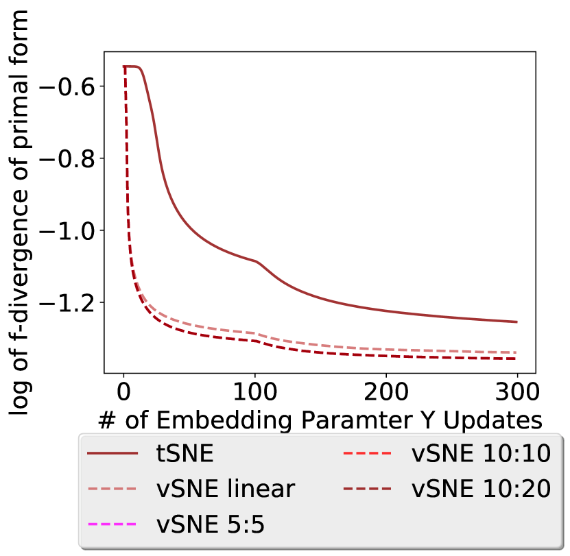
(b) NEWS

(c) CS-SNE

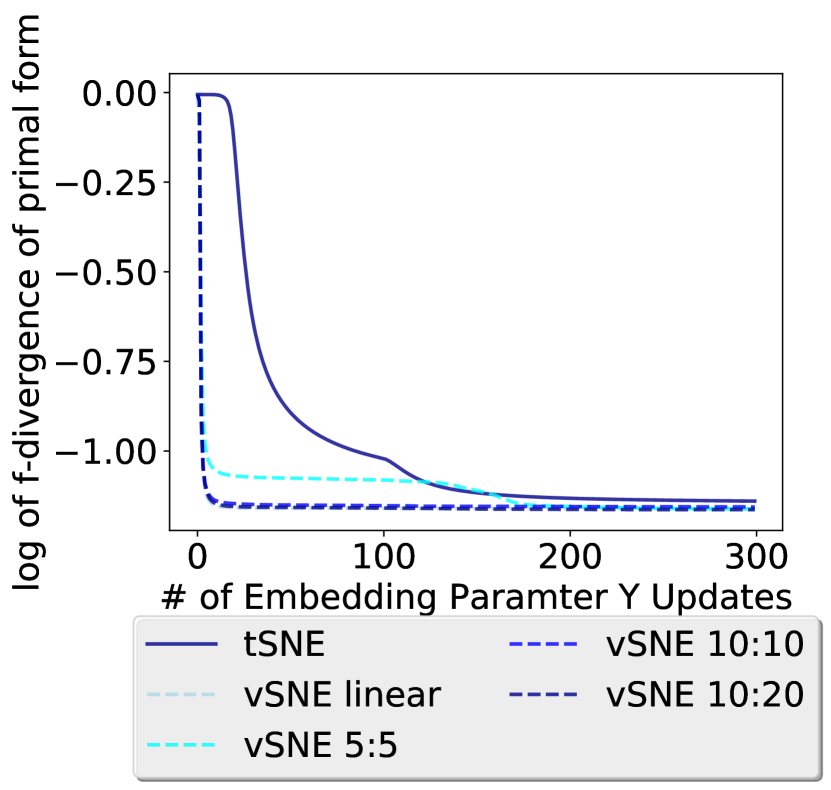
(d) MNIST1

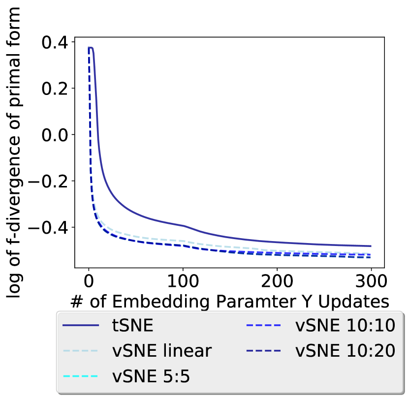
(e) NEWS

(f) JS-SNE

Figure 17: Log $ft$-SNE criterion during optimization for different discriminator network architectures of different widths on MNIST.

Figure 5b and 5c compares the results as we change the architecture of the discriminator. We experimented with a linear classifier and neural networks with 1-3 hidden layers of varying numbers of hidden units (network width). Figure 5a compares results results as we vary network width (architecture shown in Supp. Fig. 15) and Figure 5b compares results as we change network depth (architecture shown in Supp. Fig. 15). We observed that the performance was largely consistent as we changed network architecture. The results for JS and CH-SNE are shown in Supp. Fig. 17a and 17b.

5 Discussion and Related Work

Other divergences for $t$-SNE optimization have been explored previously. Perhaps the first detailed study was done by Bunte et al. [4] where they explored divergences from various families (Gamma- Bregman- and $f$-divergences) and their corresponding visualizations on some image processing datasets. Yang et al. [22] and Narayan et al. [15] recently discussed how different divergences can be used to find micro and macro relationships in data. An interesting line of work by Lee et al. [11] and Najim and Lim [14] highlights the issues of trustworthy structure discovery and multi-scale visualizations to find local and global structures.

The work by Amid et al. [2] is closely related where they study $\alpha$-divergences from an informational retrieval perspective. Our work extends it to the general class of $f$-divergences and explores the relationships between data structure and the type of divergence used.

It is worth emphasizing that no previous study makes an explicit connection between the choice of divergence and the type of structure discovery. Our work makes this explicit and should help a practitioner gain better insights about their data in the data exploration phase. Our work goes a step further and attempts to ameliorate the issues non-convex objective function in the $ft$-SNE criterion. By studying the variational dual form, we can achieve better quality (locally optimal) solutions, which would be extremely beneficial to the practitioner.

Appendix A Precision and Recall

Proof.

For KL:

$$J_{KL}(x_{i}) =\sum_{j}p_{ji}\left(\log\frac{p_{ji}}{q_{ji}}\right)$$

$$=\sum_{\begin{subarray}{c}j\neq i,\\ p_{ji}=a_{i},\\ q_{ji}=c_{i}\end{subarray}}a_{i}\log\left(\frac{a_{i}}{c_{i}}\right)\ +\sum_{\begin{subarray}{c}j\neq i,\\ p_{ji}=a_{i},\\ q_{ji}=d_{i}\end{subarray}}a_{i}\log\left(\frac{a_{i}}{d_{i}}\right)\ +\sum_{\begin{subarray}{c}j\neq i,\\ p_{ji}=b_{i},\\ q_{ji}=c_{i}\end{subarray}}b_{i}\log\left(\frac{b_{i}}{c_{i}}\right)\ +\sum_{\begin{subarray}{c}j\neq i,\\ p_{ji}=b_{i},\\ q_{ji}=d_{i}\end{subarray}}b_{i}\log\left(\frac{b_{i}}{d_{i}}\right)$$

$$=n^{i}_{TP}a_{i}\log\left(\frac{a_{i}}{c_{i}}\right)+n^{i}_{FN}a_{i}\log\left(\frac{a_{i}}{d_{i}}\right)\ n^{i}_{FP}b_{i}\log\left(\frac{b_{i}}{c_{i}}\right)+n^{i}_{TN}b_{i}\log\left(\frac{b_{i}}{d_{i}}\right)$$

where $n^{i}_{TP},n^{i}_{FN},n^{i}_{FP},n^{i}_{TN}$ are number of true positives, false negatives (missed points), false positives, and true negatives respectively for point $x_{i}$. Given that $\delta$ is close to $0$, then the coefficient of $n^{i}_{FN}$ and $n^{i}_{FP}$ dominates the other terms,

$$J_{KL} =n^{i}_{FN}a_{i}\log\left(\frac{a_{i}}{d_{i}}\right)+n^{i}_{FP}b_{i}\log\left(\frac{b_{i}}{c_{i}}\right)+O(\delta)$$

$$=n^{i}_{FN}\frac{1-\delta}{r_{i}}\log\left(\frac{1-\delta}{\delta}\frac{m-k_{i}-1}{r_{i}}\right)+n^{i}_{FP}\frac{\delta}{m-r_{i}-1}\log\left(\frac{\delta}{1-\delta}\frac{k_{i}}{m-r_{i}-1}\right)+O(\delta).$$

Again, the $\log\frac{1-\delta}{\delta}$ dominates the other logarithmic terms $\bigg{(}\log\left(\frac{m-r_{i}-1}{k_{i}}\right)$ and $\log\left(\frac{m-k_{i}-1}{r_{i}}\right)\bigg{)}$, so we have

$$J_{KL} =\left(\frac{n^{i}_{FN}}{r_{i}}(1-\delta)-\frac{n^{i}_{FP}}{m-r_{i}-1}\delta\right)\log\left(\frac{1-\delta}{\delta}\right)+O(\delta)$$

$$=\frac{n^{i}_{FN}}{r_{i}}C_{0}=(1-\text{Recall}(i))C_{0}+O(\delta)$$

where $C_{0}=\log\left(\frac{1-\delta}{\delta}\right)$.

For Reverse KL:

$$J_{RKL}(x_{i}) =-\sum_{j}q_{ji}\left(\log\frac{p_{ji}}{q_{ji}}\right)$$

$$=-\sum_{\begin{subarray}{c}j\neq i,\\ p_{ji}=a_{i},\\ q_{ji}=c_{i}\end{subarray}}c_{i}\log\left(\frac{a_{i}}{c_{i}}\right)\ -\sum_{\begin{subarray}{c}j\neq i,\\ p_{ji}=a_{i},\\ q_{ji}=d_{i}\end{subarray}}d_{i}\log\left(\frac{a_{i}}{d_{i}}\right)\ -\sum_{\begin{subarray}{c}j\neq i,\\ p_{ji}=b_{i},\\ q_{ji}=c_{i}\end{subarray}}c_{i}\log\left(\frac{b_{i}}{c_{i}}\right)\ -\sum_{\begin{subarray}{c}j\neq i,\\ p_{ji}=b_{i},\\ q_{ji}=d_{i}\end{subarray}}d_{i}\log\left(\frac{b_{i}}{d_{i}}\right)$$

$$=-n^{i}_{TP}c_{i}\log\left(\frac{a_{i}}{c_{i}}\right)-n^{i}_{FN}d_{i}\log\left(\frac{a_{i}}{d_{i}}\right)\ -n^{i}_{FP}c_{i}\log\left(\frac{b_{i}}{c_{i}}\right)-n^{i}_{TN}d_{i}\log\left(\frac{b_{i}}{d_{i}}\right)$$

where $n^{i}_{TP},n^{i}_{FN},n^{i}_{FP},n^{i}_{TN}$ are number of true positives, false negatives (missed points), false positives, and true negatives respectively for point $x_{i}$. Given that $\delta$ is close to $0$, then the coefficient of $n^{i}_{FN}$ and $n^{i}_{FP}$ dominates the other terms,

$$J_{RKL} =-n^{i}_{FN}d_{i}\log\left(\frac{a_{i}}{d_{i}}\right)-n^{i}_{FP}c_{i}\log\left(\frac{b_{i}}{c_{i}}\right)+O(\delta)$$

$$=-n^{i}_{FN}\frac{\delta}{m-k_{i}-1}\log\left(\frac{1-\delta}{\delta}\frac{m-k_{i}-1}{r_{i}}\right)-n^{i}_{FP}\frac{1-\delta}{k_{i}}\log\left(\frac{\delta}{1-\delta}\frac{k_{i}}{m-r_{i}-1}\right)+O(\delta).$$

Again, the $\log\frac{1-\delta}{\delta}$ dominates the other logarithmic terms $\bigg{(}\log\left(\frac{m-r_{i}-1}{k_{i}}\right)$ and $\log\left(\frac{m-k_{i}-1}{r_{i}}\right)\bigg{)}$, so we have

$$J_{RKL} =\left(\frac{n^{i}_{FP}}{k_{i}}(1-\delta)-\frac{n^{i}_{FN}}{m-k_{i}-1}\delta\right)\log\left(\frac{1-\delta}{\delta}\right)+O(\delta)$$

$$=\frac{n^{i}_{FP}}{r_{i}}C_{0}=(1-\text{Precision}(i))C_{0}+O(\delta)$$

where $C_{0}=\log\left(\frac{1-\delta}{\delta}\right)$.

For Jensen-Shanon :

$$J_{JS}(x_{i}) =\frac{1}{2}\left(\sum_{j}p_{ij}\log\frac{2p_{ij}}{p_{ij}+q_{ij}}+\sum_{j}q_{ij}\log\frac{2q_{ij}}{p_{ij}+q_{ij}}\right)$$

$$=-\frac{1}{2}\left(\sum_{j}p_{ij}\log\frac{p_{ij}+q_{ij}}{p_{ij}}+\sum_{j}q_{ij}\log\frac{p_{ij}+q_{ij}}{q_{ij}}+\log 4\right)$$

$$=-\frac{1}{2}\left(\sum_{j}p_{ij}\log\frac{q_{ij}}{p_{ij}}+\sum_{j}q_{ij}\log\frac{p_{ij}}{q_{ij}}+\log 4\right)$$

$$=\frac{1}{2}\left(J_{KL}(x_{i})+J_{RKL}(x_{i})+\log 4\right)$$

For Chi-Square distance:

$$J_{\text{CS}}(x_{i}) =\sum_{j}q_{ji}\left(\frac{p_{ji}}{q_{ji}}\right)^{2}$$

$$=\sum_{\begin{subarray}{c}j\neq i,\\ p_{ji}=a_{i},\\ q_{ji}=c_{i}\end{subarray}}c_{i}\left(\frac{a_{i}}{c_{i}}-1\right)^{2}\ +\sum_{\begin{subarray}{c}j\neq i,\\ p_{ji}=a_{i},\\ q_{ji}=d_{i}\end{subarray}}d_{i}\left(\frac{a_{i}}{d_{i}}-1\right)^{2}\ +\sum_{\begin{subarray}{c}j\neq i,\\ p_{ji}=b_{i},\\ q_{ji}=c_{i}\end{subarray}}c_{i}\left(\frac{b_{i}}{c_{i}}-1\right)^{2}\ +\sum_{\begin{subarray}{c}j\neq i,\\ p_{ji}=b_{i},\\ q_{ji}=d_{i}\end{subarray}}d_{i}\left(\frac{b_{i}}{d_{i}}-1\right)^{2}$$

$$=n^{i}_{TP}c_{i}\left(\frac{a_{i}}{c_{i}}-1\right)^{2}+n^{i}_{FN}d_{i}\left(\frac{a_{i}}{d_{i}}-1\right)^{2}\ +n^{i}_{FP}c_{i}\left(\frac{b_{i}}{c_{i}}-1\right)^{2}+n^{i}_{TN}d_{i}\left(\frac{b_{i}}{d_{i}}-1\right)^{2}.$$

Given that $\delta$ is near $0$, then the last term $\left(n^{i}_{TN}d_{i}\left(\frac{b_{i}}{d_{i}}-1\right)^{2}\right)$ gets eliminated. So, we have

$$J_{\text{CS}}(x_{i}) =n^{i}_{TP}c_{i}\left(\frac{a_{i}}{c_{i}}-1\right)^{2}+n^{i}_{FN}d_{i}\left(\frac{a_{i}}{d_{i}}-1\right)^{2}+n^{i}_{FP}c_{i}\left(\frac{b_{i}}{c_{i}}-1\right)^{2}+O(\delta)$$

$$=n^{i}_{TP}\frac{1-\delta}{k_{i}}\left(\frac{r_{i}}{k_{i}}-1\right)^{2}$$

$$\qquad\qquad+n^{i}_{FN}\frac{\delta}{m-k_{i}-1}\left(\frac{1-\delta}{\delta}\frac{m-k_{i}-1}{r_{i}}-1\right)^{2}+n^{i}_{FP}\frac{1-\delta}{k_{i}}\left(\frac{\delta}{1-\delta}\frac{k_{i}}{m-r_{i}-1}-1\right)^{2}+O(\delta)$$

$$=\frac{n^{i}_{TP}}{k_{i}}(1-\delta)C_{0}+\frac{n^{i}_{FN}}{r_{i}}(1-\delta)C_{1}+\frac{n^{i}_{FP}}{k_{i}}(1-\delta)+O(\delta)$$

$$=\text{Precision}(i)C_{0}+(1-\text{Precision}(i))+(1-\text{Recall}(i))C_{1}.$$

where $C_{0}=(\frac{r_{i}}{k_{i}}-1)^{2}$ and $C_{1}=\left(\frac{1-\delta}{\delta}\frac{m-k_{i}-1}{r_{i}}-2\right)$.

The proof layout is similar for Hellinger distance, except that it emphasize recall and has less strict penalities,

$$J_{\text{HL}}(x_{i}) =n^{i}_{TP}c_{i}\left(\sqrt{\frac{a_{i}}{c_{i}}}-1\right)^{2}+n^{i}_{FN}d_{i}\left(\sqrt{\frac{a_{i}}{d_{i}}}-1\right)^{2}+n^{i}_{FP}c_{i}\left(\sqrt{\frac{b_{i}}{c_{i}}}-1\right)^{2}$$

$$=n^{i}_{TP}\frac{1-\delta}{k_{i}}\left(\sqrt{\frac{r_{i}}{k_{i}}}-1\right)^{2}$$

$$\qquad+n^{i}_{FN}\frac{\delta}{m-k_{i}-1}\left(\sqrt{\frac{1-\delta}{\delta}\frac{m-k_{i}-1}{r_{i}}}-1\right)^{2}+n^{i}_{FP}\frac{1-\delta}{k_{i}}\left(\sqrt{\frac{\delta}{1-\delta}\frac{k_{i}}{m-r_{i}-1}}-1\right)^{2}+O(\delta)$$

$$=\frac{n^{i}_{TP}}{k_{i}}(1-\delta)C_{0}+\frac{n^{i}_{FN}}{r_{i}}(1-\delta)C_{1}+\frac{n^{i}_{FP}}{k_{i}}(1-\delta)C_{2}+O(\delta)$$

$$=\text{Precision}(i)C_{0}+(1-\text{Precision}(i))C_{2}+(1-\text{Recall}(i))C_{1}+O(\delta).$$

where $C_{0}=\left(\sqrt{\frac{r_{i}}{k_{i}}}-1\right)^{2}$, $C_{2}=\left(1-2\sqrt{\frac{r_{i}\delta}{1-\delta}}\right)$, and $C_{1}=\left(1-2\sqrt{\frac{k_{i}\delta}{1-\delta}}\right)$.

∎

Appendix B Variational $ft$-SNE

It is standard to relax the optimization of the variational $ft$-SNE objective function in Eq 3 by alternatively optimizing the paramters $\phi$ and $y_{1},\ldots,y_{m}$. Algorithm 1 alternatively updates $y_{1},\ldots,y_{m}$ and $\phi$. The parametric hypothesis class $\bar{\mathcal{H}}$ is parameterized by $\phi$ (for instance, $\phi$ are the weights of the deep neural network). Remark that this is not guaranteed to return the same solution as the original minimax objective in Eq 3. Thus it is possible that Algorithm 1 can find a different solution depending on the choice of $J$ and $K$ and under different measures.

Appendix C Experimental Supplementary Materials

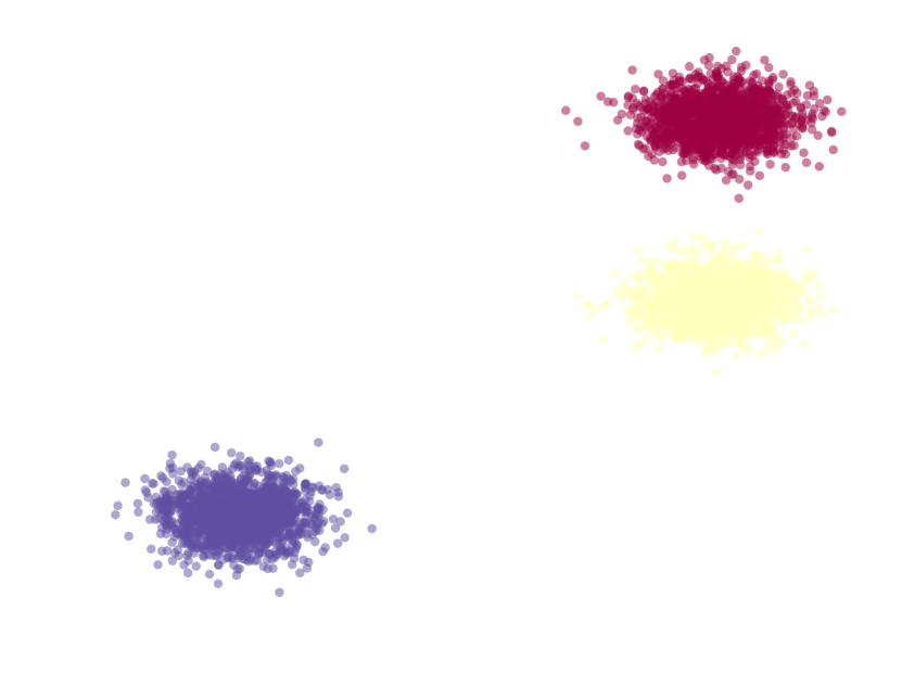
(a) Three Gaussian clusters

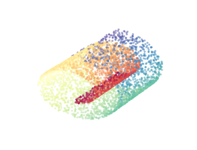
(b) Swiss Roll

Figure 6: Synthetic Datasets

Datasets. Throughout the experiments, we diversified our datasets by selecting manifold, cluster, and hierical datasets. We first experimented with two synthetic datasets, swiss roll and three Gaussian cluter datasets (see S. M. Figure 6). Thence, we conducted the set of experiments on FACE, MNIST, and 20 Newsgroups datasets. FACE and MNIST with single digits (MNIST1) fall under manifold datasets and MNIST and 20 Newsgroups fall under cluster and hierical cluster datasets.

• FACE contains 698 64 x 64 face images. The face varies smoothly with respect to light intensities and poses. The face dataset used in isomap paper [18]. We use face dataset as a manifold dataset.

• MNIST consists of 28 x 28 handwritten digits dataset with digits from 0 to 9. MNIST data points were projected down to $30$ features using PCA. We used MNIST as both clustering and manifold datasets. For clustering dataset, we used 6,000 examples of first five digits (MNIST). For manifold dataset, we used 6,000 examples of digits of ones (MNIST1).

• 20-NEWSGROUPS consists of 20 different news genres. Among 20 news genres, some of the genres fall under the same abstract categories. The 20-newsgroup data are represented using bag of words. We used 6,000 new articles that fall under thirteen categories: rec.autos, rec.motorcycles, rec.sport.baseball, rec.sport.hockey, sci.crypt, sci.electronics, sci.med, sci.space, soc.religion.christian, talk.politics.guns, talk.politics.mideast, talk.politics.misc, and talk.religion.misc. Hence, this dataset corresponds to sparse hierarchical clustering dataset.

Optimization. We use gradient decent method with momentum to optimize the $ft$-SNE. We decreased the learning rate and momentum overtime as such $\epsilon_{t+1}=\frac{\epsilon_{t}}{(1+\frac{t}{\rho})}$ and $\lambda_{t+1}=\frac{\lambda_{t}}{(1+\frac{t}{\eta})}$ where $\epsilon_{t}$ and $\lambda_{t}$ are learning rate and momentum, and $\rho$ and $\eta$ are learning rate decay and momentum decay parameters. $t$-SNE has very tiny gradients in the beginning since all the parameters are intialize in the quite small domain (the initial embeddings are drawn from the Normal distribution with zero mean and $1*e^{-4}$ standard deviation). However, once the embedding parameters spread, the gradients become relatively large compare to early stage. Thus, the learning rate and momentum require to be adjusted appropriately over different stage of optimization.

C.1 More Experimental Results : Synthetic Data Experiments

MNIST1

Face

MNIST

GENE

NEWS

SBOW

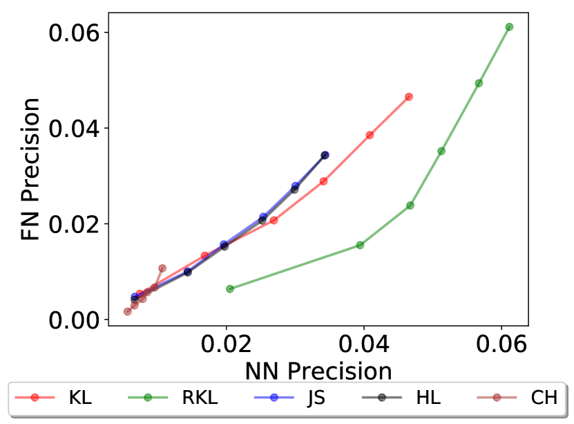
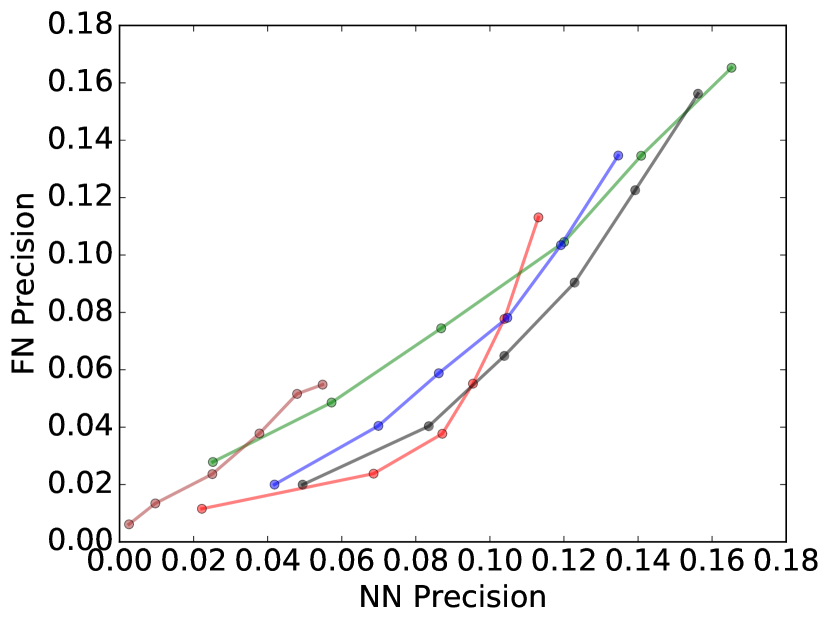
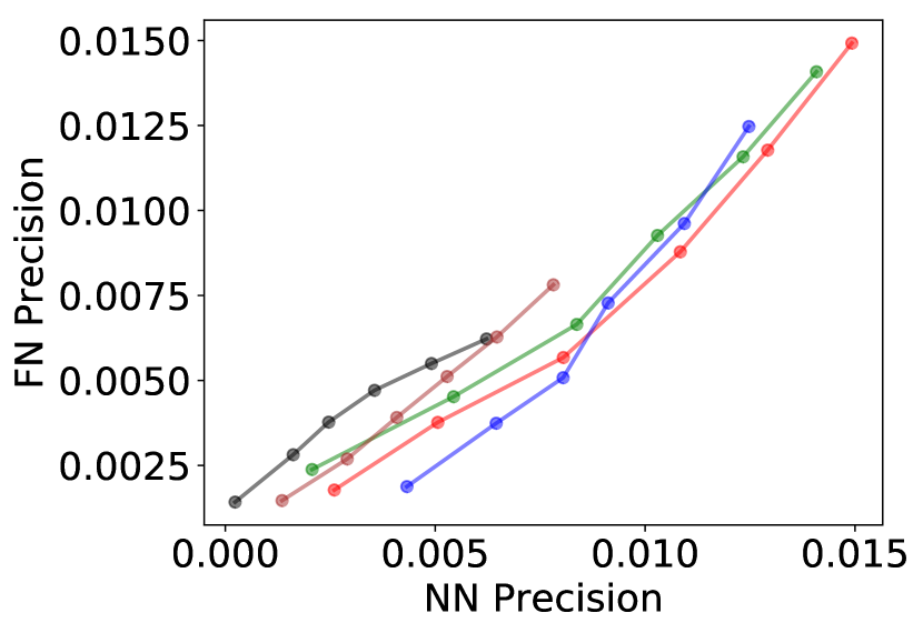
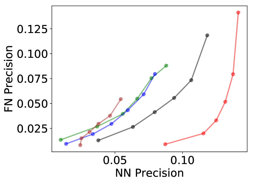
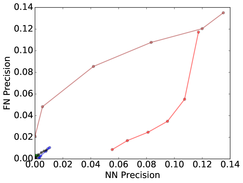
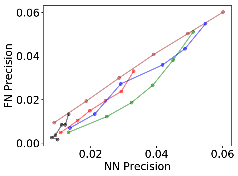
(a) FN Precision vs. NN Precision

Figure 7: Precision-Recall curves for each of the proposed algorithms on all datasets. Each row corresponds to a different dataset, each column to different quantitative criteria, and each line to a different algorithm.

(a) RKL: $\alpha=0$

(b) $\alpha=0.01$

(c) $\alpha=0.1$

(d) JS: $\alpha=0.5$

(e) KL: $\alpha=1$

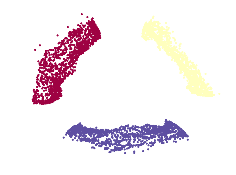
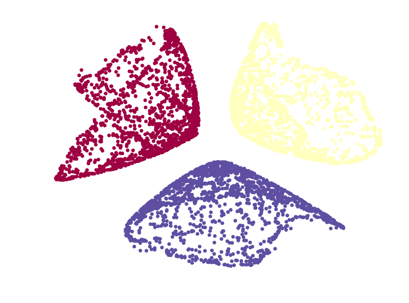
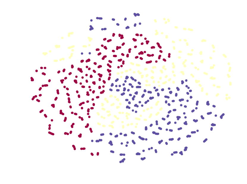
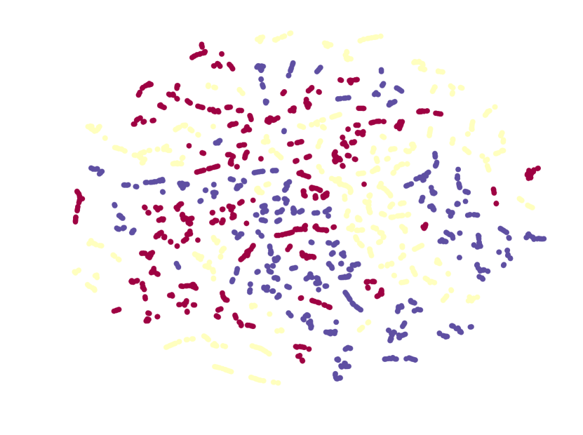
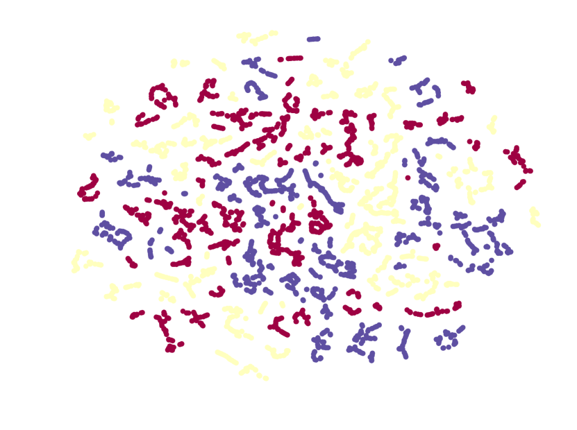
(f) Perplexity=10

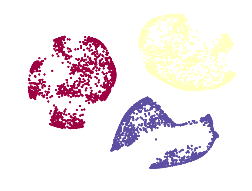
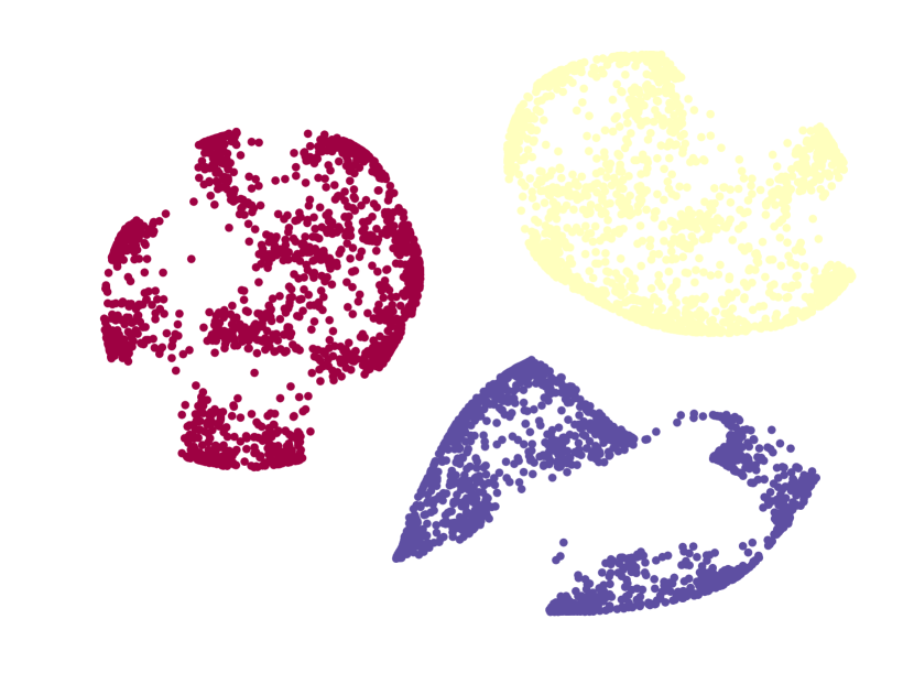
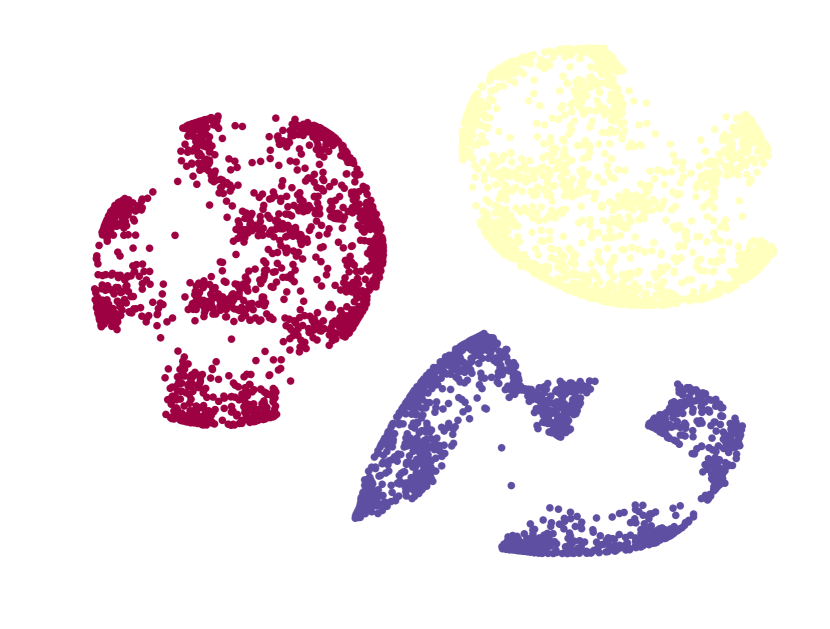
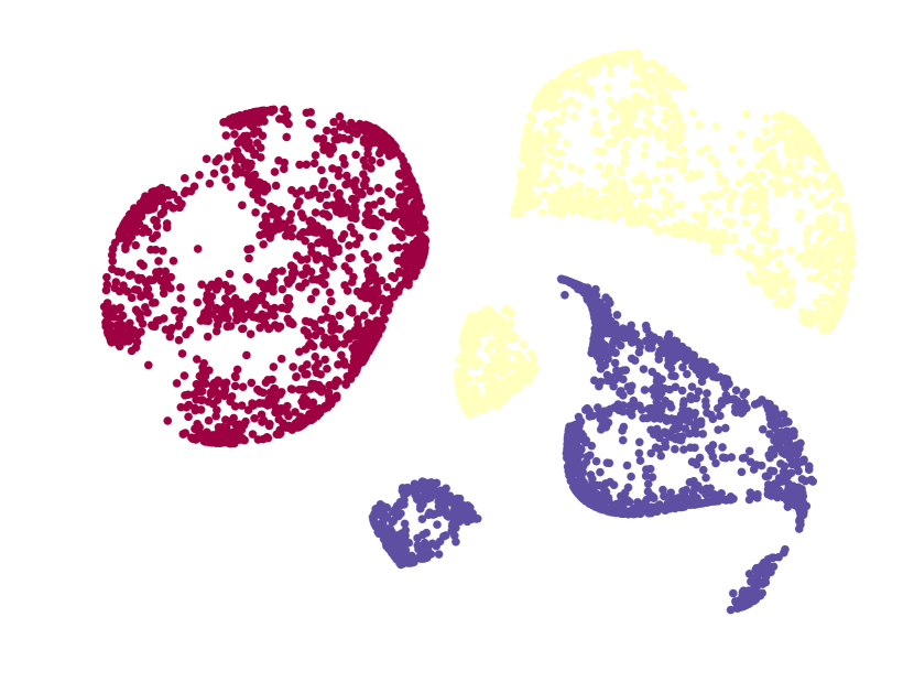
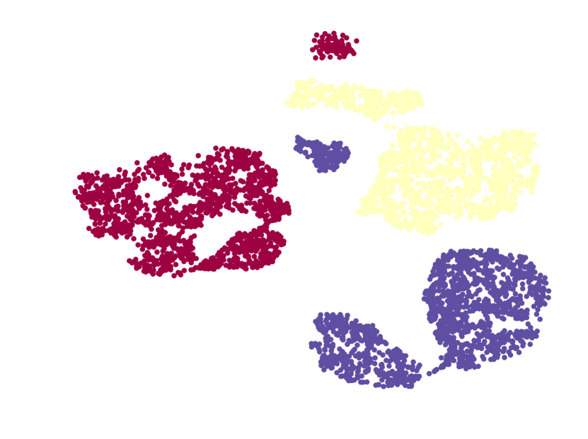
(g) Perplexity=100

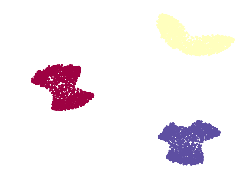
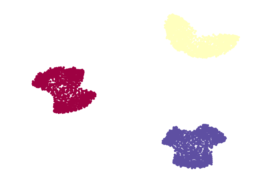
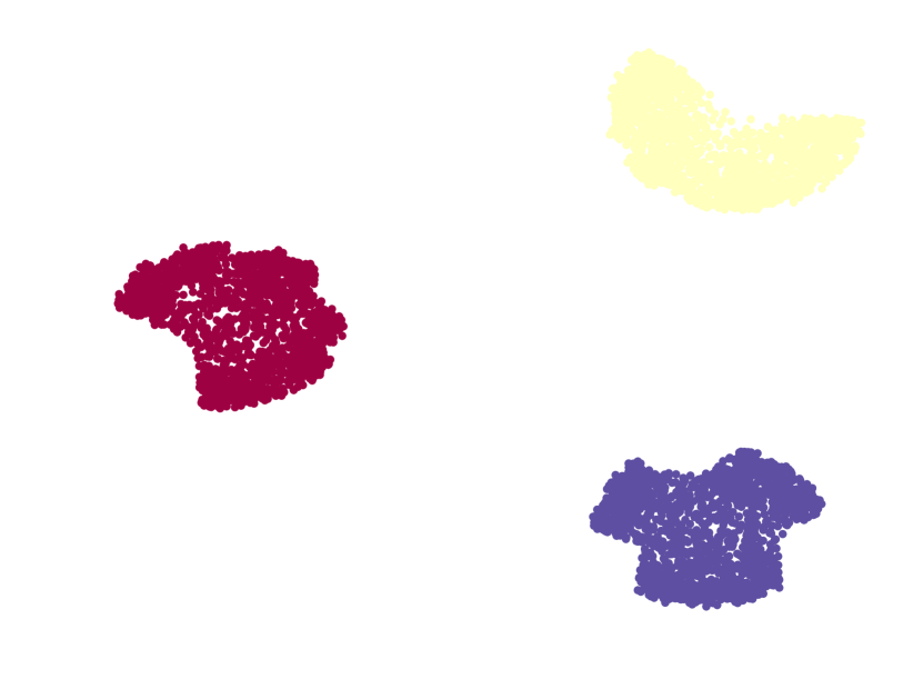
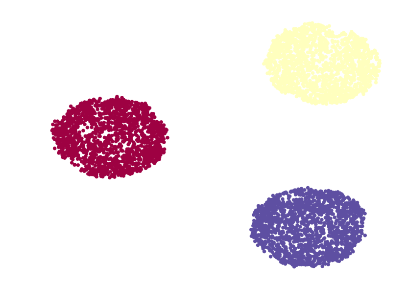
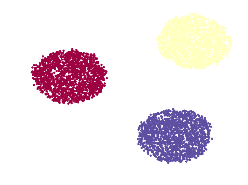
(h) Perplexity=500

Figure 8: $t$-SNE embeddings on three Gaussian clusters

(a) RKL: $\alpha=0$

(b) $\alpha=0.01$

(c) $\alpha=0.1$

(d) JS: $\alpha=0.5$

(e) KL: $\alpha=1$

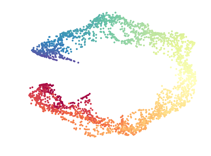
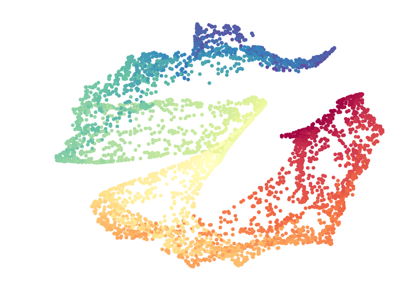
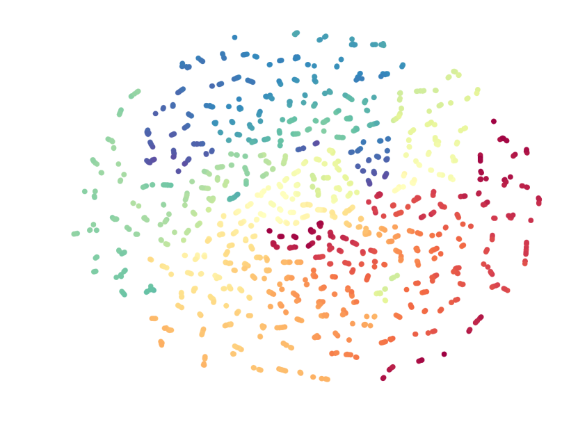
(f) Perplexity=10

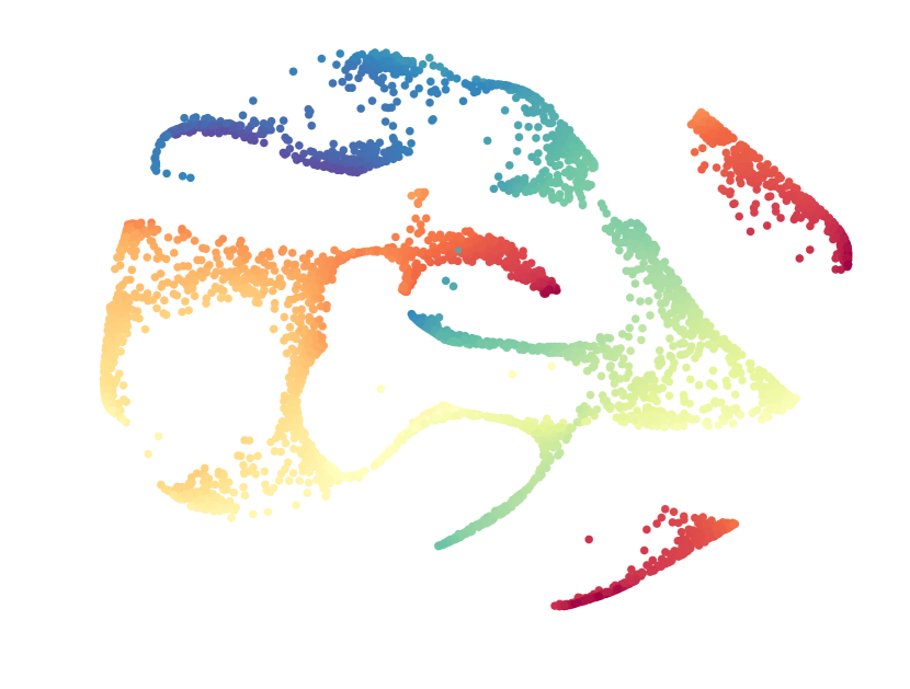
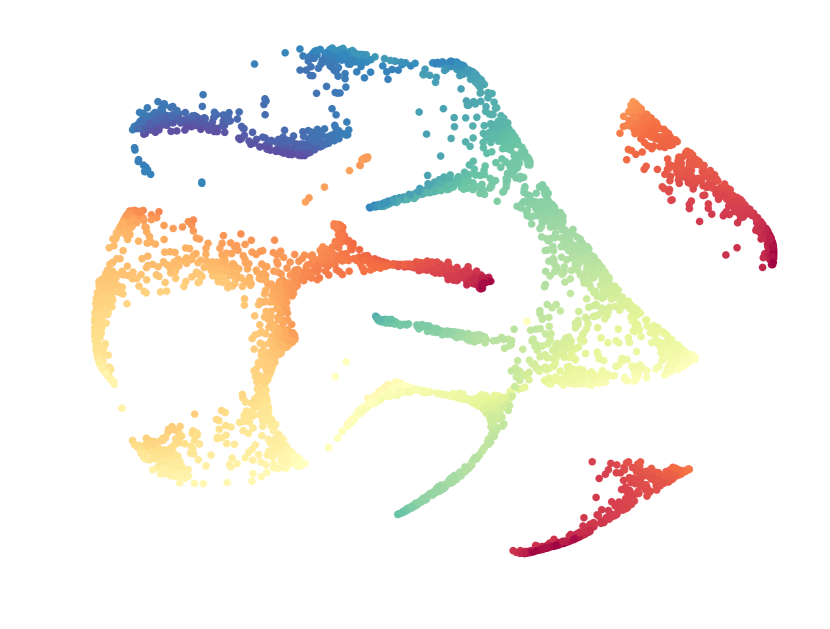
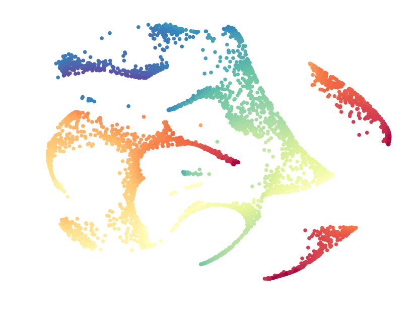
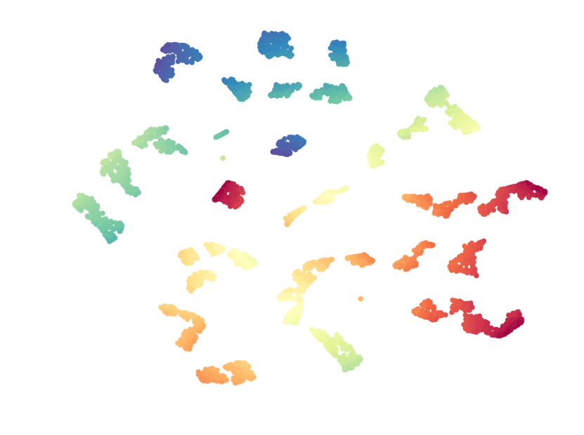
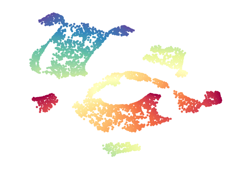
(g) Perplexity=100

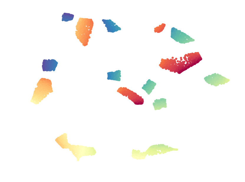
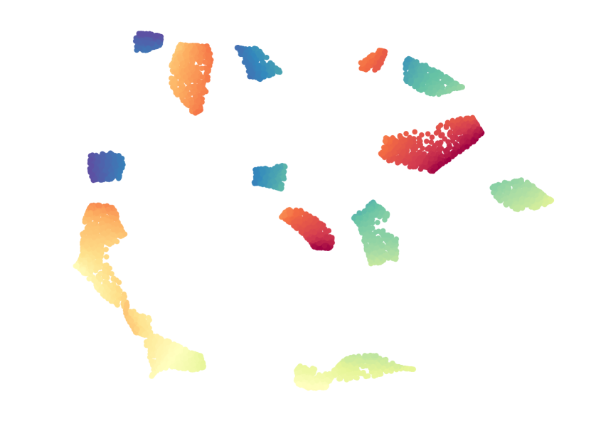
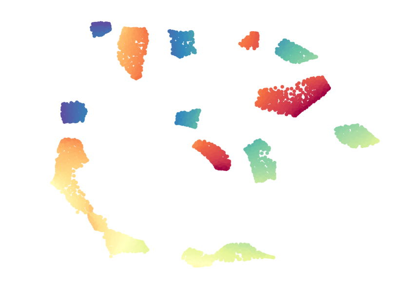
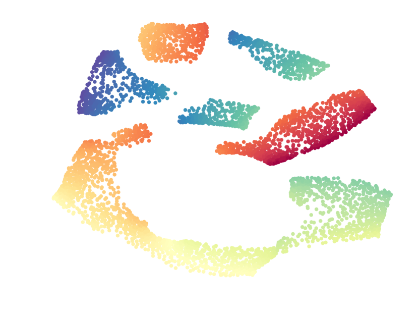
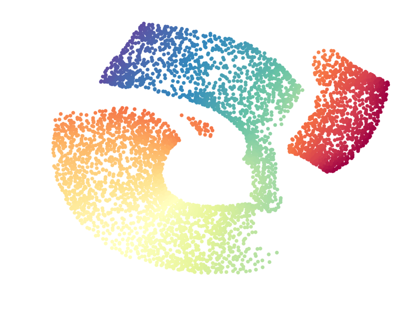
(h) Perplexity=500

Figure 9: $t$-SNE embeddings on Swiss Roll

Table 4: F-Score on X-Y MNIST

KL	RKL	JS	HL	CH
0.3524	0.4241	0.4190	0.4155	0.0922
0.4440	0.5699	0.5395	0.5332	0.1476
0.4724	0.6057	0.5570	0.5546	0.2349
0.4603	0.5687	0.5220	0.5217	0.3007
0.4407	0.5234	0.4843	0.4843	0.3222
0.4202	0.4798	0.4491	0.4503	0.3350
0.4016	0.4413	0.4189	0.4210	0.3420
0.3836	0.4090	0.3939	0.3964	0.3449
0.3667	0.3814	0.3722	0.3745	0.3446

Table 5: F-Score on X-Y FACE

KL	RKL	JS	HL	CH
0.4019	0.4186	0.4156	0.4115	0.2112
0.5648	0.6446	0.6216	0.6197	0.2919
0.6236	0.7534	0.7200	0.7146	0.3505
0.5865	0.6970	0.6793	0.6764	0.3674
0.5354	0.6207	0.6105	0.6095	0.3689
0.4870	0.5447	0.5441	0.5412	0.3642
0.4464	0.4841	0.4862	0.4826	0.3573

Table 6: F-Score on X-Y MNIST

KL	RKL	JS	HL	CH
0.4795	0.4444	0.4693	0.4494	0.4787
0.5938	0.5805	0.6006	0.5667	0.6109
0.5466	0.5872	0.5834	0.5426	0.5772
0.4891	0.5334	0.5256	0.4895	0.5200
0.4457	0.4868	0.4783	0.4494	0.4742
0.4149	0.4495	0.4409	0.4186	0.4391
0.3925	0.4180	0.4103	0.3950	0.4112
0.3749	0.3920	0.3856	0.3757	0.3879
0.3597	0.3699	0.3657	0.3595	0.3688

Table 7: F-Score on X-Y NEWS

KL	RKL	JS	HL	CH
0.3996	0.3665	0.3922	0.3989	0.2637
0.4256	0.4108	0.4328	0.4331	0.3703
0.3820	0.3933	0.4001	0.3964	0.4466
0.3387	0.3569	0.3559	0.3526	0.4633
0.3062	0.3209	0.3188	0.3163	0.4599
0.2796	0.2899	0.2877	0.2862	0.4476
0.2562	0.2626	0.2610	0.2594	0.4297
0.2346	0.2380	0.2370	0.2357	0.4076
0.2145	0.2162	0.2157	0.2148	0.3824

Table 8: F-Score on X-Y IMAGENET SBOW

KL	RKL	JS	HL	CH
0.4317	0.3411	0.3456	0.2431	0.4395
0.4686	0.3825	0.3823	0.2977	0.4889
0.4297	0.3635	0.3638	0.3157	0.4493
0.3747	0.3259	0.3280	0.3066	0.3838
0.3265	0.2932	0.2941	0.2914	0.3320
0.2867	0.2635	0.2659	0.2728	0.2919
0.2553	0.2403	0.2421	0.2532	0.2614
0.2306	0.2218	0.2222	0.2336	0.2373
0.2111	0.2065	0.2061	0.2149	0.2177

Table 9: F-Score on X-Z FACE

KL	RKL	JS	HL	CH
0.1444	0.1461	0.1482	0.1464	0.0930
0.2220	0.2318	0.2370	0.2327	0.1434
0.3012	0.3284	0.3262	0.3217	0.2043
0.3322	0.3511	0.3585	0.3524	0.2405
0.3421	0.3401	0.3652	0.3596	0.2645
0.3431	0.3267	0.3615	0.3557	0.2807
0.3396	0.3171	0.3531	0.3486	0.2915
0.3337	0.3068	0.3423	0.3384	0.2965
0.3249	0.3015	0.3278	0.3261	0.2983

Table 10: F-Score on X-Z MNIST

KL	RKL	JS	HL	CH
0.3872	0.3503	0.3810	0.3686	0.3783
0.6137	0.5269	0.6007	0.5622	0.5967
0.7238	0.6128	0.7023	0.6584	0.6884
0.7531	0.6406	0.7246	0.6958	0.7054
0.6903	0.5974	0.6649	0.6826	0.6524
0.6027	0.5379	0.5795	0.6224	0.5698
0.5277	0.4850	0.5073	0.5537	0.4989
0.4667	0.4344	0.4472	0.4940	0.4414
0.4186	0.3923	0.3994	0.4448	0.3958

Table 11: F-Score on X-Z NEWS

KL	RKL	JS	HL	CH
0.0066	0.0076	0.0074	0.0076	0.0069
0.0036	0.0041	0.0038	0.0040	0.0034
0.0018	0.0020	0.0020	0.0020	0.0018
0.0013	0.0014	0.0015	0.0015	0.0014
0.0011	0.0011	0.0012	0.0012	0.0013
0.0011	0.0010	0.0011	0.0011	0.0011
0.0010	0.0009	0.0010	0.0009	0.0011
0.0010	0.0009	0.0009	0.0009	0.0010
0.0010	0.0009	0.0009	0.0009	0.0010

Table 12: F-Score on X-Z IMAGENET SBOW

KL	RKL	JS	HL	CH
0.0063	0.0051	0.0044	0.0052	0.0043
0.0025	0.0021	0.0025	0.0027	0.0023
0.0016	0.0014	0.0017	0.0018	0.0014
0.0012	0.0013	0.0013	0.0013	0.0011
0.0010	0.0011	0.0011	0.0011	0.0010
0.0009	0.0009	0.0009	0.0009	0.0009
0.0008	0.0008	0.0008	0.0008	0.0008
0.0007	0.0007	0.0007	0.0007	0.0007
0.0006	0.0006	0.0007	0.0006	0.0007

C.2 More Experimental Results : Optimization of the primal form versus variational form (Duality Gap) Analysis

Table 13: Amount of time for $v$KL-SNE to achieve same level of loss as KL-SNE

	KL-SNE	$v$KL-SNE
Data	-	vSNE 20 hids	vSNE 10-20 hids	vSNE 5-10-20 hids
MNIST (Digit 1)	294s	230.1s	196.17s	217.3s
MNIST	1280s	1239.84s	972.72s	1171.05s
News	505.8s	2003.48s	1910.08s	1676.73s

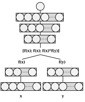
Figure 10: Discriminant Architecture

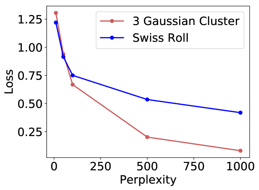
(a) KL-SNE

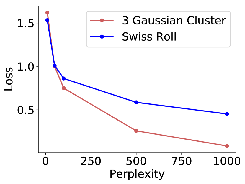
(b) JS-SNE

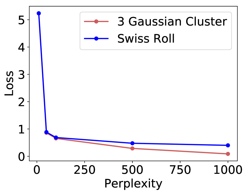
(c) RKL-SNE

Figure 12: $ft$-SNE Loss with respect to different perplexities on three Gaussian cluster and swiss roll datasets.

C.2.1 More Experimental Results with different discriminant functions

Architecture Optimizing under $vf$-SNE require having a discriminant function. Throughout the experiments, we used deep neural network the discriminator, The architecture tology is defined as $D(x_{i},x_{j})=g([f(x_{i})+f(x_{j});f(x_{i})\odot f(x_{j})])$ (depicted in S. M. Figure 10). $f(\cdot)$ is the neural network that encodes the pair of data points, $f(x)$ and $f(y)$, and $g(\cdot)$ is the neural network that takes $[f(x)+f(y);f(x)\odot f(y)]$ and outputs the score value. Our architecture is invariant to the ordering of data points (i.e., $D(x_{i},x_{j})=D(x_{j},x_{i})$). We used 10 hidden layers and 20 hidden layers for $f(\cdot)$ and $g(\cdot)$ in the experiments except when we experiments with expressibility of discriminant function.

(a) KL-SNE

Appendix D Embeddings

Figure 18 presnets the embeddings of KL-SNE and RKL-SNE. Note that KL-SNE generates spurious clusters on the bottom left of the embeddings, whereas RKL-SNE generated smooth embeddigns that captures the manifold structure. Note that in practice, we do not want to generate such a spurious cluster because the practitioners can misinterpret the visualization of the dataset.

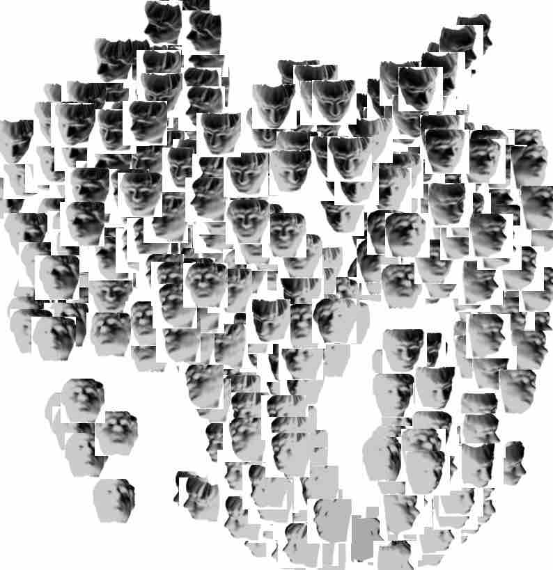
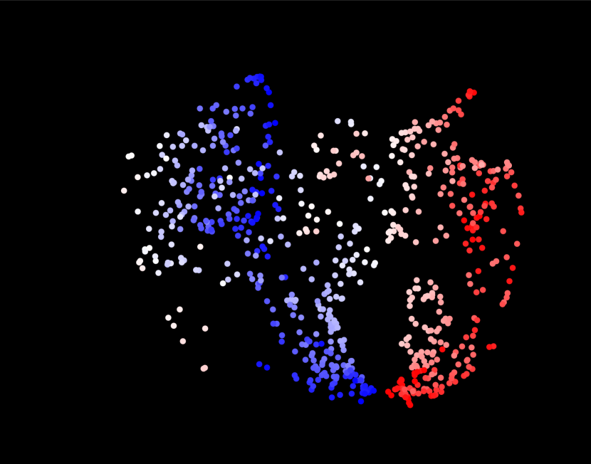
(a) RKL-SNE

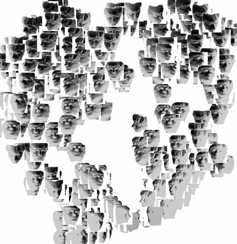
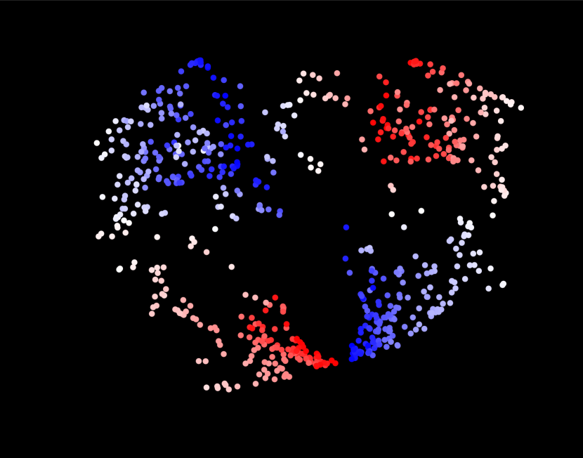
(b) RKL-SNE

Figure 18: Face Embeddings with KL and RKL-SNE

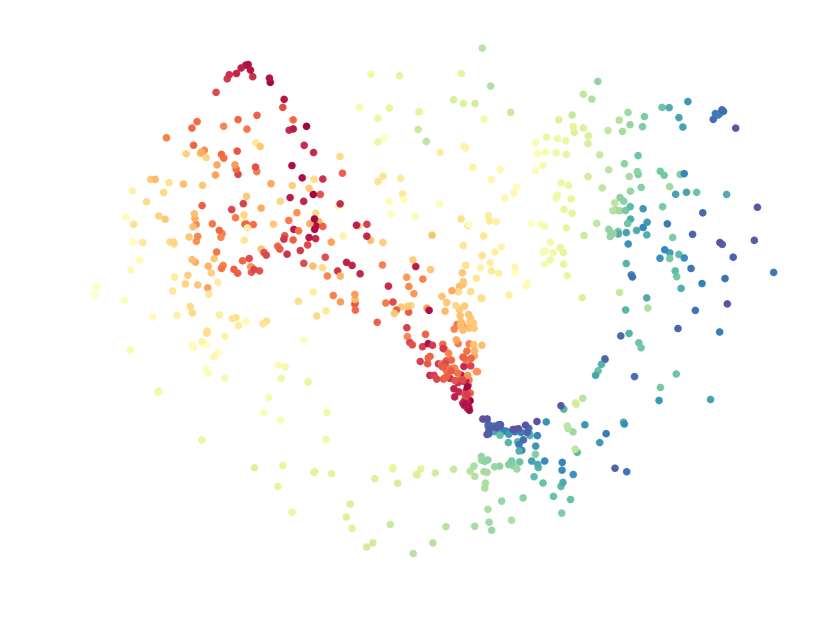
(a) KL-SNE

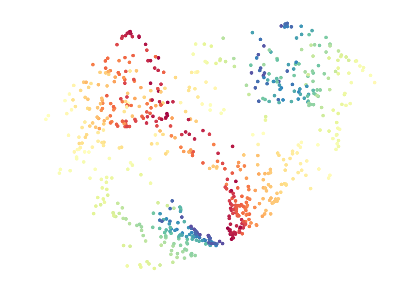
(b) RKL-SNE

(c) JS-SNE

(d) HL-SNE

(e) CH-SNE

(f) Coloured based on pose 1

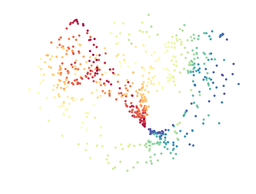
(g) KL-SNE

(h) RKL-SNE

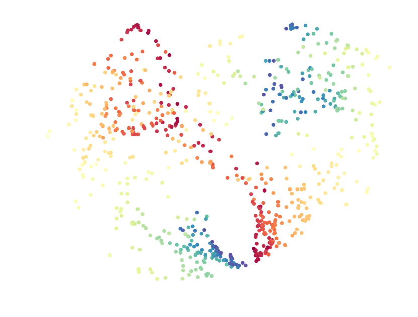
(i) JS-SNE

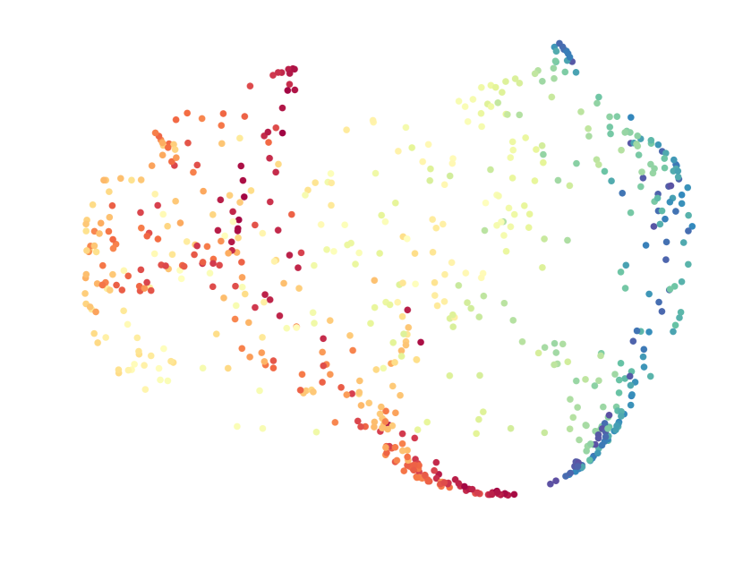
(j) HL-SNE

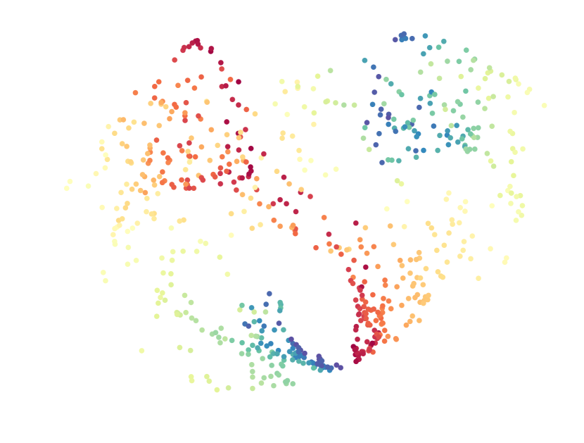
(k) CH-SNE

(l) Coloured based on pose 2

Figure 19: Face Embeddings using $ft$-SNE. Perplexity=300

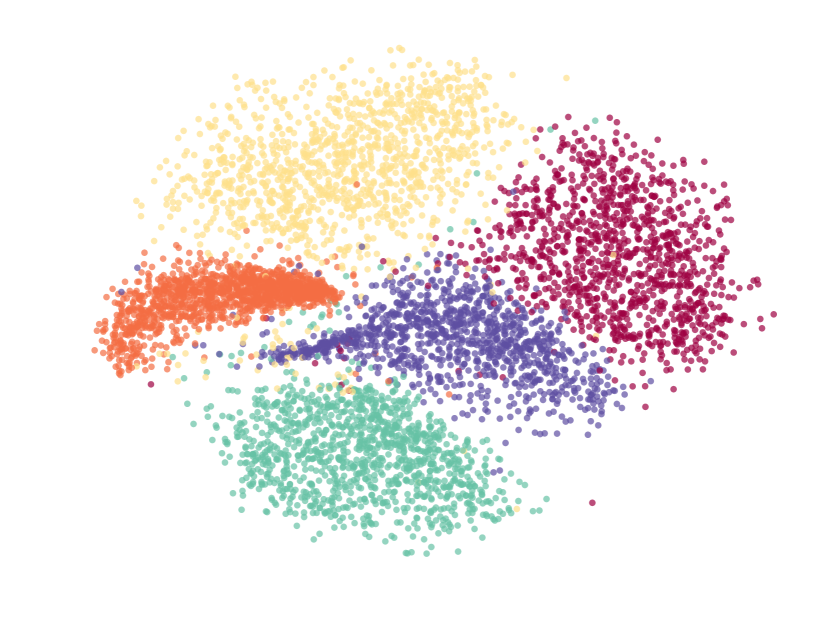
(a) KL-SNE

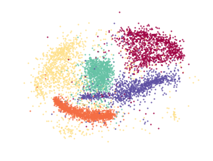
(b) RKL-SNE

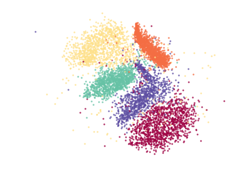
(c) JS-SNE

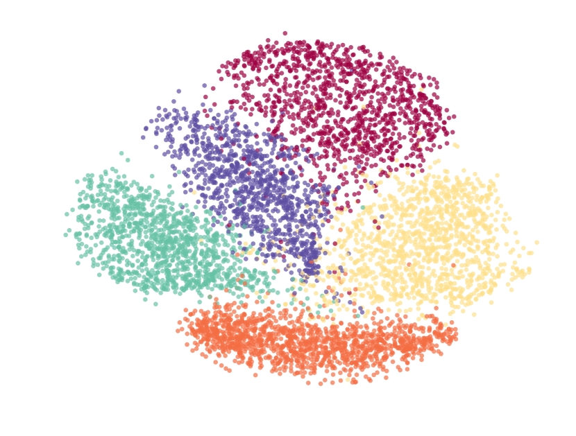
(d) HL-SNE

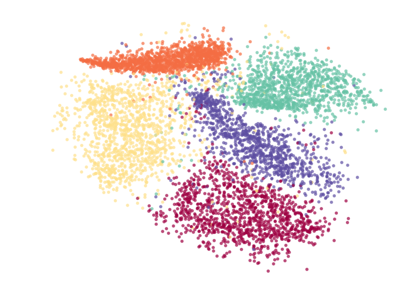
(e) CH-SNE

Figure 20: MNIST Embeddings using $f$-SNE. Perplexity: 2000 & Step: 2000

References

- Abdelmoula et al. [2014] W. Abdelmoula, K. kráková, B. Balluff, R. Carreira, E. Tolner, B.P.F. Lelieveldt, L.J.P. van der Maaten, H. Morreau, A. van den Maagdenberg, R. Heeren, L. McDonnell, and J. Dijkstra. Automatic generic registration of mass spectrometry imaging data to histology using nonlinear stochastic embedding. Analytical Chemistry, 86(18):9204–9211, 2014.
- Amid et al. [2015] Ehsan Amid, Onur Dikmen, and Erkki Oja. Optimizing the information retrieval trade-off in data visualization using -divergence. In arXiv preprint arXiv:1505.05821, 2015.
- Arora et al. [2018] Sanjeev Arora, Wei Hu, and Pravesh Kothari. An analysis of the t-SNE algorithm for data visualization. Conference on Learning Theory (COLT), 2018.
- Bunte et al. [2012] Kerstin Bunte, Sven Haase, Michael Biehl, and Thomas Villmann. Stochastic neighbor embedding (SNE) for dimension reduction and visualization using arbitrary divergences. Neurocomputing, 90:23–45, 2012.
- Ch’ng et al. [2018] Kelvin Ch’ng, Nick Vazquez, and Eshan Khatami. Unsupervised machine learning account of magnetic transitions in the hubbard model. Physical Review E, 97, 2018.
- Gashi et al. [2009] I. Gashi, V. Stankovic, C. Leita, and O. Thonnard. An experimental study of diversity with off-the-shelf antivirus engines. Proceedings of the IEEE International Symposium on Network Computing and Applications, pages 4–11, 2009.
- Hamel and Eck [2010] P. Hamel and D. Eck. Learning features from music audio with deep belief networks. Proceedings of the International Society for Music Information Retrieval Conference (ISMIR), pages 339–344, 2010.
- Jamieson et al. [2010] A.R. Jamieson, M.L. Giger, K. Drukker, H. Lui, Y. Yuan, and N. Bhooshan. Exploring nonlinear feature space dimension reduction and data representation in breast CADx with laplacian eigenmaps and t-SNE. Medical Physics, 37(1):339–351, 2010.
- Joachims [1996] Thorsten Joachims. A probabilistic analysis of the rocchio algorithm with tfidf for text categorization. Technical report, Carnegie-mellon univ pittsburgh pa dept of computer science, 1996.
- LeCun et al. [1998] Yann LeCun, Léon Bottou, Yoshua Bengio, and Patrick Haffner. Gradient-based learning applied to document recognition. Proceedings of the IEEE, 86(11):2278–2324, 1998.
- Lee et al. [2015] John A. Lee, Diego H. Peluffo-Ordóñez, and Michel Verleysen. Multi-scale similarities in stochastic neighbour embedding: Reducing dimensionality while preserving both local and global structure. Neurocomputing, 169:246–261, 2015.
- Linderman and Steinerberger [2017] George C. Linderman and Stefan Steinerberger. Clustering with t-SNE, provably. In arXiv preprint arXiv:1706.02582, 2017.
- Mahfouz et al. [2015] A. Mahfouz, M. van de Giessen, L.J.P. van der Maaten, S. Huisman, M.J.T. Reinders, M.J. Hawrylycz, and B.P.F. Lelieveldt. Visualizing the spatial gene expression organization in the brain through non-linear similarity embeddings. Methods, 73:79–89, 2015.
- Najim and Lim [2014] Safa A. Najim and Ik Soo Lim. Trustworthy dimension reduction for visualization different data sets. Information Sciences, 278:206–220, 2014.
- Narayan et al. [2015] Karthik Narayan, Ali Punjani, and Pieter Abbeel. Alpha-beta divergences discover micro and macro structures in data. International Conference on Machine Learning (ICML), 2015.
- Nguyen et al. [2008] XuanLong Nguyen, Martin J. Wainwright, and Michael I. Jordan. Estimating divergence functionals and the likelihood ratio by penalized convex risk minimization. In Proceedings of the Neural Information Processing Systems (NIPS), 2008.
- Nowozin et al. [2016] Sebastian Nowozin, Botond Cseke, and Ryota Tomioka. -GAN: Training generative neural samplers using variational divergence minimization. In arXiv preprint arXiv:1606.00709, 2016.
- Tenenbaum et al. [2000] Joshua. B. Tenenbaum, Vin. de Silva, and John. C. Langford. A global geometric framework for nonlinear dimensionality reduction. Science, 290:2319–2323, 2000.
- van der Maaten and Hinton [2008] Laurens van der Maaten and Geoffrey Hinton. Visualizing data using t-SNE. Journal of Machine Learning Research (JMLR), 9:2579–2605, 2008.
- Venna et al. [2010] Jarkko Venna, Jaakko Peltonen, Kristian Nybo, Helena Aidos, and Samuel Kaski. Information retrieval perspective to nonlinear dimensionality reduction for data visualization. Journal of Machine Learning Research (JMLR), 11:451–490, 2010.
- Weinstein et al. [2013] John N Weinstein, Eric A Collisson, Gordon B Mills, Kenna R Mills Shaw, Brad A Ozenberger, Kyle Ellrott, Ilya Shmulevich, Chris Sander, Joshua M Stuart, Cancer Genome Atlas Research Network, et al. The cancer genome atlas pan-cancer analysis project. Nature genetics, 45(10):1113, 2013.
- Yang et al. [2014] Zhirong Yang, Jaakko Peltonen, and Samuel Kaski. Optimization equivalence of divergences improves neighbor embedding. International conference on machine learning (ICML), 2014.
- Zhang et al. [2007] J. Zhang, M. Marszalek, S. Lazebnik, and C. Schmid. Local features and kernels for classification of texture and object categories: a comprehensive study. International Journal of Computer Vision (IJCV), 2007.