Regulating spin reversal in dipolar systems by the quadratic Zeeman effect

Abstract

A mechanism is advanced suggesting the resolution of the dichotomy of long-lived spin polarization storage versus fast spin reversal at the required time. A system of atoms or molecules is considered interacting through magnetic dipolar forces. The constituents are assumed to possess internal structure allowing for the generation of the alternating-current quadratic Zeeman effect, whose characteristics can be efficiently regulated by quasiresonant dressing. The sample is connected to an electric circuit producing a feedback field acting on spins. By switching on and off the alternating-current quadratic Zeeman effect it is possible to realize spin reversals with a required delay time. The suggested technique of regulated spin reversal can be used in quantum information processing and spintronics.

I Introduction

Dipolar interactions are widespread in nature being typical of many biological systems Cameretti_1 ; Waigh_2 , polymers Barford_3 , magnetic nanomolecules Kahn_4 ; Barbara_5 ; Caneschi_6 ; Yukalov_7 ; Yukalov_8 ; Yukalov_32 and magnetic nanoclusters Kodama_9 ; Hadjipanayis_10 ; Yukalov_11 ; Yukalov_12 . Many dipolar atoms and molecules can form self-arranged lattices or can be organized in lattice structures with the help of external fields Griesmaier_13 ; Baranov_14 ; Baranov_15 ; Gadway_16 ; Yukalov_17 . Dipolar interactions are also typical of ensembles of quantum dots Escobar_36 and quantum nanowires Corona_37 that possess many properties similar to atoms, because of which they are often called artificial atoms Birman_38 .

Here we consider lattices formed by constituents possessing magnetic dipolar moments. These constituents are supposed to enjoy internal structure that can be used for inducing the alternating-current quadratic Zeeman effect by applying quasiresonant linearly polarized light populating internal spin states Cohen_18 ; Santos_19 ; Jensen_20 ; Paz_21 . The alternating-current quadratic Zeeman effect can also be induced by quasiresonant linearly polarized microwave driving field populating internal hyperfine states Gerbier_22 ; Leslie_23 ; Bookjans_24 . It is important that the optically induced quadratic Zeeman effect can also be realized with atoms or molecules without hyperfine structure. Such a quasiresonant driving exerts quadratic Zeeman shift along the field polarization axis. This shift is described by a parameter $q_{Z}$ that does not depend on a stationary external field. By using either positive or negative detuning, the sign of the parameter can be varied. The optically or microwave induced quadratic Zeeman effect can be easily manipulated and rapidly adjusted, thus providing an efficient tool for regulating the properties of the sample.

One of the properties of spin systems, which is extremely important for spintronics, as well as for quantum information processing, is the possibility of fast spin reversal. At the same time, this property is in contradiction with the other important requirement of being able to keep for long time a fixed spin polarization. This is because one can fix spin polarization for sufficiently long time by choosing materials with a high magnetic anisotropy. However the latter is the major obstacle for realizing fast spin reversal. The same dilemma of a well fixed spin polarization versus fast spin reversal, which arises in spintronic techniques, also exists in quantum information processing, where keeping a fixed spin polarization is necessary for creating memory devices, while one needs fast spin reversal for the efficient functioning of such devices. The proposed devices for realizing quantum computing are also based on spin systems Bernien_39 ; Zhang_40 .

Generally, spin reversal in magnetic materials can be induced by inverting a static external magnetic field Shuty_33 . However this is a rather slow process requiring sufficiently strong fields. A faster reversal can be realized by applying alternating electromagnetic fields, such as produced by lasers Deb_34 ; Shelukhin_35 .

In the present paper, we advance a novel mechanism that, from one side, allows us to keep for a long time a fixed spin polarization, while, from the other side, provides an efficient tool for realizing a fast spin reversal at any time needed. This mechanism suggests a resolution of the dilemma of the fixed spin polarization versus fast spin reversal. We show that this can be done for dipolar magnetic systems by employing the alternating-current quadratic Zeeman effect.

II Scheme of suggested setup

The suggested setup is as follows. A magnetic sample is inserted into a magnetic coil with inductance $L$, containing $n$ turns and having length $l$ and cross-section area $A_{coil}$. The coil is a part of an electric circuit also including capacity $C$ and resistance $R$. The coil axis is along the axis $x$. A constant external magnetic field $B_{0}$ is directed along the axis $z$. The moving spins of the magnetic sample induce in the coil electric current $j$ defined by the Kirchhoff equation

$$L\;\frac{dj}{dt}+Rj+\frac{1}{C}\int_{0}^{t}j(t^{\prime})\;dt^{\prime}=-\;\frac{d\Phi}{dt}\;,$$ (1)

in which the electromotive force is caused by the magnetic flux

$$\Phi=\frac{4\pi}{c}\;nA_{coil}\;\eta_{f}\;m_{x}$$

formed by the component of the moving magnetic moment of density $m_{x}$. Here $\eta_{f}=V/V_{eff}$ is a filling factor being the ratio of the sample volume $V$ to the effective volume of the coil $V_{eff}$. The coil inductance is

$$L=4\pi\;\frac{n^{2}A_{coil}}{c^{2}l}\;.$$

The circuit natural frequency, circuit damping, and quality factor are

$$\omega=\frac{1}{\sqrt{LC}}\;,\qquad\gamma=\frac{R}{2L}\;,\qquad Q=\frac{\omega L}{R}\;.$$ (2)

The electric current of the coil produces the magnetic field

$$H=\frac{4\pi n}{cl}\;j$$ (3)

directed along the coil axis. This field, being induced by moving spins, acts back on the spins, because of which it is called the feedback field. The overall scheme of the suggested setup is shown in Fig. 1.

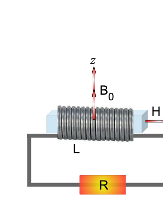
Figure 1: Scheme of suggested setup, as is explained in the text.

III Operator equations of motion

We consider a system of constituents (atoms or molecules) interacting through dipolar forces. The advantage of dealing with such systems is twofold. From one side, as is emphasized in the Introduction, systems with dipolar interactions are widespread in nature, hence there exists a variety of materials with rather different properties. That is, the system parameters can be varied in a wide range. From the other side, dipolar interactions are much weaker then exchange interactions, because of which the quadratic Zeeman effect can effectively influence the properties of the system. While in hard magnetic materials, such as ferromagnets and antiferromagnets, the alternating-current Zeeman effect can be too weak, as compared to the energy of exchange interactions, so that the alternating-current Zeeman effect would not produce the desired regulation of spin dynamics.

The Hamiltonian of the dipolar lattice system of $N$ sites, each possessing a total spin $S$ and characterized by the spin operator ${\bf S}_{j}$, with $j=1,2,\ldots,N$, is the sum of the Zeeman term $\hat{H}_{Z}$ and the part $\hat{H}_{D}$ describing dipolar interactions. Generally, dipolar lattices can also include single-site magnetic anisotropy. So that the total Hamiltonian is the sum

$$\hat{H}=\hat{H}_{Z}+\hat{H}_{D}+\hat{H}_{A}\;.$$ (4)

The Zeeman Hamiltonian contains a linear Zeeman term and a quadratic Zeeman term induced by the alternating-current quasiresonant light Cohen_18 ; Santos_19 ; Jensen_20 ; Paz_21

$$\hat{H}_{Z}=-\mu_{S}\sum_{j}{\bf B}\cdot{\bf S}_{j}+q_{Z}\sum_{j}(S_{j}^{z})^{2}\;,$$ (5)

where $\mu_{S}=-g_{S}\mu_{B}$, with $g_{S}$ being the spin $g$-factor and $\mu_{B}$, Bohr magneton, while ${\bf B}$ is an external magnetic field acting on spins. The parameter $q_{Z}$ of the quadratic Zeeman effect, induced by a linearly polarized driving field coupling internal states, does not depend on the field ${\bf B}$. The axis $z$ is assumed to be the polarization axis of the driving field. This parameter $q_{Z}$, for an alternating field that is quasiresonant with an internal transition and that is linearly polarized along the axis $z$, can be written (see Appendix A) in the form

$$q_{Z}=-\frac{\hbar\Omega^{2}}{4\Delta_{res}}\;,$$ (6)

where $\Omega$ is the driving Rabi frequency and $\Delta_{res}$ is the detuning from an internal transition related to spin or hyperfine structure. The parameter $q_{Z}$ can be tailored at high resolution and rapidly adjusted. By applying either positive or negative detuning, the sign of this parameter can be made either positive or negative.

The dipolar Hamiltonian reads as

$$\hat{H}_{D}=\frac{1}{2}\sum_{i\neq j}\;\sum_{\alpha\beta}D_{ij}^{\alpha\beta}S_{i}^{\alpha}S_{j}^{\beta}\;,$$ (7)

where the dipolar tensor

$$D_{ij}^{\alpha\beta}=\frac{\mu_{S}^{2}}{r_{ij}^{3}}\;\left(\delta_{\alpha\beta}-3n_{ij}^{\alpha}n_{ij}^{\beta}\right)\exp(-\varkappa r_{ij})\;,$$ (8)

generally, includes the screening effect, with the screening parameter $\varkappa$. The screening of dipolar forces does exist in some materials Jonscher_25 ; Jonscher_41 ; Jonscher_42 ; Tarasov_43 ; Yukalov_26 , while if it is not important, one can set $\varkappa$ to zero. The following consideration does not depend on the existence or absence of screening, which is mentioned here only for generality. Here

$$r_{ij}\equiv|\;{\bf r}_{ij}\;|\;,\qquad{\bf n}_{ij}\equiv\frac{{\bf r}_{ij}}{r_{ij}}\;,\qquad{\bf r}_{ij}={\bf r}_{i}-{\bf r}_{j}\;.$$

The total external magnetic field ${\bf B}$ includes a constant field $B_{0}$ directed along the $z$-axis. And the sample is assumed to be placed inside a magnetic coil of an electric circuit, so that the coil produces a magnetic feedback field $H$ directed along the $x$-axis,

$${\bf B}=B_{0}{\bf e}_{z}+H{\bf e}_{x}\;.$$ (9)

The single-site magnetic anisotropy term can be written Bedanta_44 in the form

$$\hat{H}_{A}=-\sum_{j}D(S_{j}^{z})^{2}\;.$$ (10)

With the use of the ladder operators $S_{j}^{\pm}=S_{j}^{x}\pm iS_{j}^{y}$, the Zeeman term transforms into

$$\hat{H}_{Z}=\sum_{j}\left[-\mu_{S}B_{0}S_{j}^{z}\;-\;\frac{1}{2}\;\mu_{S}H\left(S_{j}^{+}+S_{j}^{-}\right)+q_{Z}\left(S_{j}^{z}\right)^{2}\right]\;.$$ (11)

And the dipolar part becomes

$$\hat{H}_{D}=\frac{1}{2}\sum_{i\neq j}\left[a_{ij}\left(S_{i}^{z}S_{j}^{z}-\;\frac{1}{2}\;S_{i}^{+}S_{j}^{-}\right)+\right.$$

$$\left.+b_{ij}S_{i}^{+}S_{j}^{z}+b^{*}_{ij}S_{i}^{-}S_{j}^{z}+2c_{ij}S_{i}^{+}S_{j}^{z}+2c^{*}_{ij}S_{i}^{-}S_{j}^{z}\right]\;,$$ (12)

in which the interaction coefficients are

$$a_{ij}\equiv D_{ij}^{zz}\;,\qquad b_{ij}\equiv\frac{1}{4}\left(D_{ij}^{xx}-D_{ij}^{yy}-2iD_{ij}^{xy}\right)\;,$$

$$c_{ij}\equiv\frac{1}{2}\left(D_{ij}^{xz}-iD_{ij}^{yz}\right)\;.$$ (13)

Writing down the equations of motion for the spin operators, we introduce the notation for the Zeeman frequency

$$\omega_{0}\equiv-\frac{\mu_{S}B_{0}}{\hbar}>0\;.$$ (14)

Also we define the quantities

$$\xi_{i}\equiv\frac{1}{\hbar}\sum_{j}\left(a_{ij}S_{j}^{z}+c_{ij}^{*}S_{j}^{-}+c_{ij}S_{j}^{+}\right)$$ (15)

and

$$\varphi_{i}\equiv\frac{1}{\hbar}\sum_{j}\left(\frac{a_{ij}}{2}\;S_{j}^{-}-2b_{ij}S_{j}^{+}-2c_{ij}S_{j}^{z}\right)$$ (16)

describing local dipolar fields acting on spins. And we introduce the effective force

$$f_{j}\equiv-i\left(\frac{\mu_{S}H}{\hbar}+\varphi_{j}\right)\;.$$ (17)

With the above notations, we obtain the spin equations for the transverse spin

$$\frac{dS_{j}^{-}}{dt}=-i(\omega_{0}+\xi_{j})S_{j}^{-}+f_{j}S_{j}^{z}\;-$$

$$-\;\frac{i}{\hbar}\;(q_{Z}-D)\left(S_{j}^{-}S_{j}^{z}+S_{j}^{z}S_{j}^{-}\right)$$ (18)

and for the spin $z$-component,

$$\frac{dS_{j}^{z}}{dt}=-\;\frac{1}{2}\left(f_{j}^{+}S_{j}^{-}+S_{j}^{+}f_{j}\right)\;.$$ (19)

The spin operators in the Heisenberg representation depend on time $t$, which is not explicitly shown for the compactness of notations. At the initial moment of time, the sample is assumed to be polarized, so that the statistical average of the spin $z$-component is nonzero, $\langle S_{j}^{z}(0)\rangle\neq 0$.

IV Dipolar spin waves

Spin waves are known to exist in ferromagnets and antiferromagnets, where spins interact through exchange interactions Akhiezer_27 ; Kalinikos_62 ; Lvov_63 ; Gurevich_64 ; Verba_65 ; Lisenkov_66 . Here we show that spin waves can also exist in the systems with pure dipolar interactions in the presence of quadratic Zeeman effect. These spin waves are called dipolar, since they arise in a sample with purely dipolar interactions, without exchange interactions.

It is necessary to emphasize that the detailed study of spin waves is not our aim here. But what is important is to show that they do exist. Their existence is important because it is the spin waves that trigger spin motion from a nonequilibrium state.

We keep in mind self-organized spin waves caused by dipolar interactions, but not induced by external forces, so that at the initial time, no rotation is imposed on the system,

$$\langle S_{j}^{-}(0)\rangle=\langle S_{j}^{+}(0)\rangle=0\;,$$ (20)

and the feedback field has not yet appeared, that is $H=0$.

Spin waves are small oscillations around the average spin values, which is described by representing the spin operators in the form

$$S_{j}^{\alpha}=\langle S_{j}^{\alpha}\rangle+\delta S_{j}^{\alpha}\;.$$ (21)

Due to the property of the dipolar tensor, the interaction functions (13) satisfy the equality

$$\sum_{j}a_{ij}=\sum_{j}b_{ij}=\sum_{j}c_{ij}=0\;.$$ (22)

Therefore, for an ideal lattice, where the statistical average does not depend on the lattice index, the local fields (15) and (16) are actually formed by spin waves, since

$$\xi_{i}=\frac{1}{\hbar}\sum_{j}\left(a_{ij}\delta S_{j}^{z}+c_{ij}\delta S_{j}^{+}+c_{ij}^{*}\delta S_{j}^{-}\right)\;,$$

$$\varphi_{i}=\frac{1}{\hbar}\sum_{j}\left(\frac{a_{ij}}{2}\;\delta S_{j}^{z}-2b_{ij}\delta S_{j}^{+}-2c_{ij}\delta S_{j}^{z}\right)\;.$$ (23)

Substituting expression (21) into the equations of motion, it is necessary to be cautious with respect to the last term in Eq. (18), taking into account that this term is exactly zero for spin $1/2$. Then we use the representation Yukalov_7 ; Yukalov_8 ; Yukalov_11 ; Yukalov_28

$$S_{j}^{-}S_{j}^{z}+S_{j}^{z}S_{j}^{-}=\left(2-\;\frac{1}{S}\right)\langle S_{j}^{z}\rangle S_{j}^{-}$$ (24)

that is exact for $S=1/2$ and is asymptotically exact for large spins, when $S\rightarrow\infty$.

Separating in the evolution equations the terms of different orders with respect to small spin deviations, in zero order, we have the equations

$$\frac{d}{dt}\;\langle S_{j}^{-}\rangle=-i\omega_{s}\langle S_{j}^{-}\rangle\;,\qquad\frac{d}{dt}\;\langle S_{j}^{z}\rangle=0\;,$$ (25)

where the effective frequency of spin rotation is

$$\omega_{s}\equiv\omega_{0}+\left(2-\;\frac{1}{S}\right)\;\frac{q_{Z}-D}{\hbar}\;\langle S_{j}^{z}\rangle\;.$$ (26)

The first equation gives

$$\langle S_{j}^{-}(t)\rangle=\langle S_{j}^{-}(0)\rangle\;e^{-i\omega_{s}t}\;.$$

In view of the initial condition (20), it follows that

$$\langle S_{j}^{-}\rangle=0\;,\qquad S_{j}^{-}=\delta S_{j}^{-}\;.$$ (27)

And the second of equations (25) shows that $\langle S_{j}^{z}\rangle=const$.

To first order with respect to the spin deviations, we find

$$\frac{d}{dt}\;\delta S_{j}^{-}=-i\omega_{s}\delta S_{j}^{-}-i\varphi_{j}\langle S_{j}^{z}\rangle\;,\qquad\frac{d}{dt}\;\delta S_{j}^{z}=0\;.$$ (28)

Because of the initial condition $\delta S_{j}^{z}(0)=0$, the above equations give $\delta S_{j}^{z}(t)=0$.

Invoking the Fourier transform for the ladder spin operators

$$S_{j}^{\pm}=\sum_{k}S_{k}^{\pm}\exp(\mp i{\bf k}\cdot{\bf r}_{j})$$

and for the interaction functions $a_{ij}$ and $b_{ij}$,

$$a_{ij}=\frac{1}{N}\sum_{k}a_{k}\exp(i{\bf k}\cdot{\bf r}_{ij})\;,$$

$$b_{ij}=\frac{1}{N}\sum_{k}b_{k}\exp(i{\bf k}\cdot{\bf r}_{ij})\;,$$

we reduce the first of equations (28) to the form

$$\frac{d}{dt}\;S_{k}^{-}=-iA_{k}S_{k}^{-}+iB_{k}S_{k}^{+}\;,$$ (29)

in which

$$A_{k}\equiv\omega_{s}+\frac{a_{k}}{2\hbar}\;\langle S_{j}^{z}\rangle\;,\qquad B_{k}\equiv\frac{2b_{k}}{\hbar}\;\langle S_{j}^{z}\rangle\;.$$ (30)

Looking for the solution

$$S_{k}^{-}=u_{k}e^{-i\omega_{k}t}+v_{k}^{*}e^{i\omega_{k}t}\;,$$ (31)

we obtain the spectrum of spin waves

$$\omega_{k}=\sqrt{A_{k}^{2}-|\;B_{k}\;|^{2}}\;.$$ (32)

Considering the long-wave limit, when $k\rightarrow 0$, we keep in mind that the wavelength $\lambda=2\pi/k$ is much larger than the interspin distance but smaller than the sample size. Then the spectrum has the form

$$\omega_{k}\simeq|\;\omega_{s}\;|\left[1-\;\frac{\langle S_{j}^{z}\rangle}{4\hbar\omega_{s}}\;\sum_{\langle ij\rangle}a_{ij}({\bf k}\cdot{\bf r}_{ij})^{2}\right]\;.$$ (33)

Here $<ij>$ implies the summation over the nearest neighbors.

Generally, the spectrum is well defined when $|A_{k}|>|B_{k}|$, which yields the stability condition

$$\left|\;\omega_{s}+\frac{a_{k}}{2\hbar}\;\langle S_{j}^{z}\rangle\;\right|\;\geq\;\left|\;\frac{2b_{k}}{\hbar}\;\langle S_{j}^{z}\rangle\;\right|\;.$$ (34)

Explicitly, this condition reads as

$$\left|(2S-1)q_{Z}+\frac{S}{\langle S_{j}^{z}\rangle}\;\hbar\omega_{0}+\frac{S}{2}\;a_{k}-(2S-1)D\right|\geq 2S|b_{k}|\;.$$

This means that spin waves exist when the Zeeman frequency $\omega_{0}$ and the parameter $q_{Z}$ of the quadratic Zeeman effect are sufficiently large, such that condition (34) be valid. The quadratic Zeeman effect can stabilize dipolar spin waves Yukalov_45 . As is clear, the existence of dipolar interactions is also crucial.

The occurrence of spin waves is very important, since they serve as a triggering mechanism initiating spin motion after the system has been prepared in an initial nonequilibrium state Yukalov_8 ; Yukalov_28 ; Yukalov_29 .

V Averaged equations of motion

Let us consider the temporal behavior of the averaged quantities, the transverse spin polarization function

$$u\equiv\frac{1}{SN}\sum_{j=1}^{N}\;\langle S_{j}^{-}\rangle\;,$$ (35)

coherence intensity

$$w\equiv\frac{1}{SN(N-1)}\sum_{i\neq j}^{N}\;\langle S_{i}^{+}S_{j}^{-}\rangle\;,$$ (36)

and the longitudinal spin polarization

$$s\equiv\frac{1}{SN}\sum_{j=1}^{N}\;\langle S_{j}^{z}\rangle\;.$$ (37)

Notice that if one resorts to the standard mean-field approximation, then the averages of the local fields (15) and (16), because of property (22), become zero,

$$\langle\xi_{j}\rangle=\langle\varphi_{j}\rangle=0\;.$$

Thus the influence of the dipolar interactions would be lost. However these interactions are principally important, since they are necessary for the existence of spin waves triggering the initial spin motion.

To take the dipolar interactions into account, we employ a more refined stochastic mean-field approximation Yukalov_8 ; Yukalov_28 ; Yukalov_30 . In the process of averaging over the spin variables, we set the notation

$$\left\langle\frac{1}{N}\sum_{j=1}^{N}\xi_{j}S_{j}^{\alpha}\right\rangle=\xi_{S}\frac{1}{N}\sum_{j=1}^{N}\;\langle S_{j}^{\alpha}\rangle\;,$$

$$\left\langle\frac{1}{N}\sum_{j=1}^{N}\varphi_{j}S_{j}^{\alpha}\right\rangle=\varphi_{S}\frac{1}{N}\sum_{j=1}^{N}\;\langle S_{j}^{\alpha}\rangle\;,$$ (38)

where $\xi_{S}$ and $\varphi_{S}$ are treated as stochastic variables related to local spin-wave fluctuations.

Realizing statistical averaging over the spin variables, we use the mean-field approximation for the spin correlation functions

$$\langle S_{i}^{\alpha}S_{j}^{\beta}\rangle=\langle S_{i}^{\alpha}\rangle\langle S_{j}^{\beta}\rangle\qquad(i\neq j)$$ (39)

corresponding to spins at different lattice sites. And for the single-site term, we employ the decoupling following from Eq. (20),

$$\langle S_{j}^{\alpha}S_{j}^{\beta}+S_{j}^{\beta}S_{j}^{\alpha}\rangle=\left(2-\;\frac{1}{S}\right)\langle S_{j}^{\alpha}\rangle\langle S_{j}^{\beta}\rangle\;,$$ (40)

which is exact for $S=1/2$ and asymptotically exact for $S\rightarrow\infty$.

The stochastic local fields $\xi_{S}$ and $\varphi_{S}$ are defined as random variables satisfying the stochastic averaging conditions

$$\langle\langle\xi_{S}(t)\rangle\rangle=\langle\langle\varphi_{S}(t)\rangle\rangle=0\;,$$

$$\langle\langle\xi_{S}(t)\xi_{S}(t^{\prime})\rangle\rangle=2\gamma_{3}\delta(t-t^{\prime})\;,$$

$$\langle\langle\xi_{S}(t)\varphi_{S}(t^{\prime})\rangle\rangle=\langle\langle\varphi_{S}(t)\varphi_{S}(t^{\prime})\rangle\rangle=0\;,$$

$$\langle\langle\varphi^{*}_{S}(t)\varphi_{S}(t^{\prime})\rangle\rangle=2\gamma_{3}\delta(t-t^{\prime})\;,$$ (41)

in which $\gamma_{3}$ is the relaxation rate caused by fluctuating spins interacting through dipolar forces. To evaluate the value of $\gamma_{3}$, we may notice that, in view of Eqs. (41), the rate $\gamma_{3}$ can be represented as

$$\gamma_{3}=\left|\;\int_{0}^{\infty}\langle\langle\xi_{S}(t)\xi_{S}(0)\rangle\rangle dt\;\right|\;.$$ (42)

The fluctuating field $\xi_{S}(t)$ behaves according to the law

$$\xi_{S}(t)\propto\gamma_{2}\exp\{-i(\omega_{s}-i\gamma_{2})t\}\;,$$

where $\omega_{s}$ is the effective spin rotation frequency (26) and

$$\gamma_{2}=\frac{1}{\hbar}\;\rho\mu_{S}^{2}S$$ (43)

is the dipolar transverse attenuation rate, in which $\rho\equiv N/V$ is average spin density, with $V$ being the sample volume. The effective spin-rotation frequency (26), that reads as

$$\omega_{s}=\omega_{0}+(2S-1)\;\frac{q_{Z}-D}{\hbar}\;s\;,$$ (44)

can be represented as

$$\omega_{s}=\omega_{0}(1+As)\;,$$ (45)

where the dimensionless parameter

$$A\equiv(2S-1)\;\frac{q_{Z}-D}{\hbar\omega_{0}}$$ (46)

plays the role of an effective magnetic anisotropy renormalized by quadratic Zeeman effect.

From the integral (42), we find

$$\gamma_{3}\cong\frac{\gamma_{2}^{2}}{\sqrt{\omega_{s}^{2}+\gamma_{2}^{2}}}\;.$$ (47)

The effective force (17), under averaging over spins, becomes

$$f=-i\left(\frac{\mu_{S}H}{\hbar}+\varphi_{S}\right)\;.$$ (48)

In the equations of motion, we take into account the existence of the transverse spin attenuation rate $\gamma_{2}$ and the longitudinal attenuation rate $\gamma_{1}$.

Finally, averaging Eqs. (18) and (19), we derive the equations for the transverse polarization function

$$\frac{du}{dt}=-i(\omega_{s}+\xi_{S}-i\gamma_{2})u+fs\;,$$ (49)

coherence intensity

$$\frac{dw}{dt}=-2\gamma_{2}w+(u^{*}f+f^{*}u)s\;,$$ (50)

and the longitudinal spin polarization

$$\frac{ds}{dt}=-\;\frac{1}{2}\;(u^{*}f+f^{*}u)-\gamma_{1}(s-s_{\infty})\;,$$ (51)

where $s_{\infty}$ is an equilibrium (or stationary) spin polarization.

VI Feedback magnetic field

According to the setup mentioned in Sec. II, the sample is inserted into a coil of an electric circuit. Therefore, moving spins induce electric current in the coil, which is described by the Kirchhoff equation. In turn, this current creates a feedback magnetic field inside the effective coil volume $V_{eff}$. Such a coupling with a resonance electric circuit induces in the system the so-called radiation damping Purcell_46 ; Bloembergen_47 ; Yukalov_48 ; Chen_49 ; Krishnan_50 . The feedback magnetic field satisfies the equation Yukalov_7 ; Yukalov_8 ; Yukalov_28 ; Yukalov_29

$$\frac{dH}{dt}+2\gamma H+\omega^{2}\int_{0}^{t}H(t^{\prime})\;dt^{\prime}=-4\pi\eta_{f}\;\frac{dm_{x}}{dt}$$ (52)

following form the Kirchhoff equation. Here $\gamma$ is the circuit ringing rate, $\omega$ is the circuit natural frequency, and $\eta_{f}$ is the filling factor $\eta_{f}=V/V_{eff}$. The electromotive force is created by the motion of spins forming the magnetic moment with the effective density

$$m_{x}=\frac{\mu_{S}}{V}\sum_{j=1}^{N}\;\langle S_{j}^{x}\rangle\;.$$

Equation (52) can be rewritten Yukalov_7 ; Yukalov_8 ; Yukalov_28 ; Yukalov_29 as the integral equation

$$H=-4\pi\int_{0}^{t}G(t-t^{\prime})\dot{m}_{x}(t^{\prime})\;dt^{\prime}\;,$$ (53)

in which

$$\dot{m}_{x}=\frac{N}{2V_{eff}}\;\mu_{S}S\;\frac{d}{dt}\;(u^{*}+u)\;,$$

the transfer function is

$$G(t)=\left[\cos(\omega_{eff}t)-\;\frac{\gamma}{\omega_{eff}}\;\sin(\omega_{eff}t)\right]e^{-\gamma t}\;,$$

with the effective frequency

$$\omega_{eff}\equiv\sqrt{\omega^{2}-\gamma^{2}}\;.$$

The electric circuit can be tuned close to the Zeeman frequency $\omega_{0}$, so that the detuning be small,

$$\left|\;\frac{\Delta}{\omega}\;\right|\ll 1\qquad(\Delta\equiv\omega-\omega_{0})\;.$$ (54)

And, as usual, all attenuations are supposed to be small, such that

$$\frac{\gamma}{\omega}\ll 1\;,\quad\frac{\gamma_{1}}{\omega_{0}}\ll 1\;,\quad\frac{\gamma_{2}}{\omega_{0}}\ll 1\;,\quad\frac{\gamma_{3}}{\omega_{0}}\ll 1\;.$$ (55)

The coupling between the magnetic coil of the electric circuit and the sample is characterized by the coupling rate

$$\gamma_{0}\equiv\frac{\pi}{\hbar}\;\rho\eta_{f}\mu_{S}^{2}S=\pi\eta_{f}\gamma_{2}\;,$$ (56)

which is close to $\gamma_{2}$, if the volumes of the sample and coil are close to each other. Solving Eq. (53) by an iterative procedure, to first order with respect to the coupling rate, we find

$$\frac{\mu_{S}H}{\hbar}=i(uX-X^{*}u^{*})\;,$$ (57)

where the coupling function is

$$X=\gamma_{0}\omega_{s}\left[\frac{1-\exp\{-i(\omega-\omega_{s})t-\gamma t\}}{\gamma+i(\omega-\omega_{s})}\right.\;+$$

$$+\;\left.\frac{1-\exp\{-i(\omega+\omega_{s})t-\gamma t\}}{\gamma-i(\omega+\omega_{s})}\right]\;.$$ (58)

When $\omega_{s}>0$, the first, quasiresonant, term in the coupling function prevails over the second, since

$$\left(\frac{\omega-|\omega_{s}|}{\omega+|\omega_{s}|}\right)^{2}<1\;.$$

By the same reason, the second term is larger than the first, if $\omega_{s}<0$. Both these cases can be summarized in the expression

$$X\cong\gamma_{0}\omega_{s}\;\frac{1-\exp(-i\Delta_{s}t-\gamma t)}{\gamma+i\Delta_{s}{\rm sign}\omega_{s}}=$$

$$=\frac{\gamma\gamma_{0}\omega_{s}}{\gamma^{2}+\Delta^{2}}\;\left\{1-\left(\cos(\Delta_{s}t)-\delta_{s}\sin(\Delta_{s}t)\right)e^{-\gamma t}\right.\;-$$

$$-\;\left.i\left[\delta_{s}-\left(\sin(\Delta_{s}t)+\delta_{s}\cos(\Delta_{s}t)\right)e^{-\gamma t}\right]\right\}\;,$$ (59)

where

$$\Delta_{s}\equiv\omega-|\;\omega_{s}\;|=\omega-\omega_{0}|\;1+As\;|\;,$$

$$\delta_{s}\;\equiv\;\frac{\Delta_{s}}{\gamma}\;{\rm sign}\;\omega_{s}\;.$$ (60)

VII Regulating spin reversal

Substituting the feedback field $H$ into Eq. (49) gives the equation

$$\frac{du}{dt}=-i\Omega u-i\xi_{S}u-i\varphi_{S}s-X^{*}u^{*}s\;,$$ (61)

where

$$\Omega=\omega_{s}-i(\gamma_{2}-Xs)\;.$$

From Eqs. (49) to (51) it follows that the functional variable $u$ can be classified as fast, while the variables $w$ and $s$ as slow. This allows us to employ the scale separation approach Yukalov_8 ; Yukalov_28 ; Yukalov_30 that is a variant of the averaging techniques. To this end, we solve equation (61) for the fast variable $u$ treating there the slow variables $w$ and $s$ as quasi-integrals of motion, which yields

$$u=u_{0}\exp\left\{-i\Omega t-i\int_{0}^{t}\xi_{S}(t^{\prime})\;dt^{\prime}\right\}-$$

$$-is\int_{0}^{t}\varphi_{S}(t^{\prime})\exp\left\{-i\Omega(t-t^{\prime})-i\int_{t^{\prime}}^{t}\xi_{S}(t^{\prime\prime})\;dt^{\prime\prime}\right\}dt^{\prime}\;.$$ (62)

The nonresonant counter-rotating term of order $\gamma_{2}/\omega_{0}$ is omitted here. Then we substitute the feedback field $H$ and the fast variable $u$ into equations (50) and (51) for the slow variables $w$ and $s$ and average these equations over time and over the stochastic variables $\xi_{S}$ and $\phi_{S}$. This results in the equations for the guiding centers

$$\frac{dw}{dt}=2\gamma_{2}w(\alpha s-1)+2\gamma_{3}s^{2}$$ (63)

and

$$\frac{ds}{dt}=-\alpha\gamma_{2}w-\gamma_{3}s-\gamma_{1}(s-s_{\infty})\;,$$ (64)

with the coupling function

$$\alpha\equiv\frac{{\rm Re}X}{\gamma_{2}}=\frac{g\gamma^{2}}{\gamma^{2}+\Delta_{s}^{2}}\;(1+As)\times$$

$$\times\left\{1-\left[\cos(\Delta_{s}t)-\delta_{s}\sin(\Delta_{s}t)\right]e^{-\gamma t}\right\}\;,$$ (65)

in which

$$g\equiv\frac{\gamma_{0}\omega_{0}}{\gamma\gamma_{2}}$$ (66)

is the dimensionless coupling parameter characterizing the coupling between the sample and the electric circuit.

Analyzing equations (63) and (64), we take into account that the dipolar relaxation rate $\gamma_{3}$ is smaller then transverse attenuation rate $\gamma_{2}$, and the longitudinal attenuation rate $\gamma_{1}$ is usually much smaller than $\gamma_{2}$. Measuring time in units of $1/\gamma_{2}$, we come to the equations

$$\frac{dw}{dt}=2w(\alpha s-1)+2\;\frac{\gamma_{3}}{\gamma_{2}}\;s^{2}\;,$$

$$\frac{ds}{dt}=-\alpha w-\;\frac{\gamma_{3}}{\gamma_{2}}\;s\;.$$ (67)

Assume that the system is polarized at the initial time, but no coherence from external sources is imposed, so that the initial conditions are

$$w(0)=0\;,\qquad s(0)=s_{0}\;.$$ (68)

The external magnetic field $B_{0}$ at the initial time is directed along the $z$ axis, so that the system is in a nonequilibrium state.

The regulation of spin dynamics is based on the possibility of varying in time the parameter $q_{z}$ of the alternating-current quadratic Zeeman effect. The value of this parameter can be varied in a rather wide range. For example, dipolar lattices, organized by means of laser beams Griesmaier_13 ; Baranov_14 ; Baranov_15 ; Gadway_16 ; Yukalov_17 have the mean interatomic distance $a\sim(10^{-5}-10^{-4})$ cm, hence the average density $\rho\sim(10^{12}-10^{15})$ cm^-3. For the magnetic moments $\mu_{S}\sim 10\mu_{B}$, the dipolar transverse rate (42) is $\gamma_{2}\sim(10-10^{4})$ s^-1. And the value $|q_{Z}|/\hbar$ can reach $10^{5}$s^-1, as can be inferred from Refs. Cohen_18 ; Santos_19 ; Jensen_20 ; Paz_21 .

There may happen two situations.

(i) First, if the dipolar system has no single-site anisotropy, then one can create a nonzero parameter $q_{Z}$ for the required time, say between zero and $\tau$, during which the initial spin polarization is preserved due to the nonzero value of parameter (46) that equals

$$A_{0}=(2S-1)\;\frac{q_{Z}}{\hbar\omega_{0}}\qquad(0\leq t<\tau)\;.$$

After this, one switches off the quadratic Zeeman effect sending $q_{Z}$ to zero, hence making zero the parameter $A$. This corresponds to the temporal behavior

$$A(t)=\left\{\begin{array}[]{ll}A_{0},{}&~{}0\leq t<\tau\\ 0,{}&~{}t\geq\tau\end{array}\right.\;.$$ (71)

(ii) A similar procedure can be realized when the single-site anisotropy parameter $D$ is not zero. Then one can either keep $q_{Z}$ zero, if the value of $D$ is sufficient for freezing the initial spin direction, or create a negative value of $q_{Z}$ for increasing the effective anisotropy to the needed magnitude. After the required time $\tau$, one should switch on the quadratic Zeeman effect so that to compensate the value of $D$, thus sending $A$ to zero.

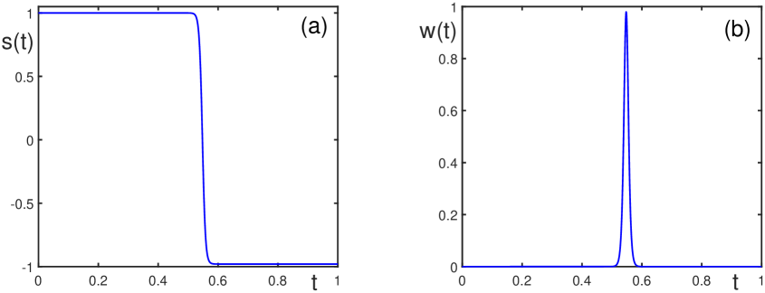
Figure 2: Longitudinal spin polarization (a) and coherence intensity (b) as functions of time measured in units of $1/\gamma_{2}$. A single spin reversal for the parameters $\gamma/\gamma_{2}=10$, $\omega=\omega_{0}=1000\gamma_{2}$, $A_{0}=1$, and $\tau=0.5/\gamma_{2}$.

Numerical solutions to Eqs. (67) are presented in Fig. 2, where we set $\gamma/\gamma_{2}=10$, $\omega=\omega_{0}=1000\gamma_{2}$, and $g=100$. For the delay time, we take $\tau=0.5/\gamma_{2}$, which can be about $10^{-3}-1$ s. The delay time can be taken much longer. As we have checked, under the chosen parameters, the delay time $\tau$, during which the spin polarization $s$ practically does not change, can reach $100/\gamma_{2}$, which amounts to $0.1-10$ s. The polarization reversal is very fast, being approximately equal $\tau_{p}\approx 1/gs_{0}\gamma_{2}$, which makes $10^{-7}-10^{-3}$ s. The polarization reversal is accompanied by a coherent pulse, shown in Fig.2b and corresponding to spin superradiance Yukalov_31 . In that way, we achieve the desired goal, being able to keep for long time a fixed longitudinal spin polarization, while quickly reversing it as soon as we need.

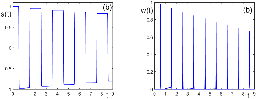
Figure 3: Sequence of longitudinal spin reversals (a) realized by inverting the external magnetic field at the moments of the dimensionless time $t_{n}=(n+1)\tau$, measured in units of $1/\gamma_{2}$, and the related sequence of superradiant bursts (b). The parameters are as in Fig. 2.

Moreover, it is straightforward to repeat the spin reversal several times by inverting the external magnetic field $B_{0}$ during the stage of frozen spin, which implies the change of $\omega_{s}$ by $-\omega_{s}$. This procedure, illustrated in Fig. 3, goes as follows. The value of $A$ is kept nonzero during the time interval $0\leq t<\tau_{1}$. At the moment of time $\tau_{1}$, by regulating the quadratic Zeeman effect, the value of $A$ is sent to zero. Thus the first reversal occurs, as in Fig. 2. The value of $A$ is kept zero till some time $t_{1}$. At this time, the external field $B_{0}$ is inverted and $A$ is set to a nonzero value, which is kept nonzero till the time $t_{1}+\tau_{2}$. At the moment of time $t_{1}+\tau_{2}$ the parameter $A$ is switched off, which results in the second spin reversal. And then the process is repeated as many times as necessary. The values $t_{n}$ and $\tau_{n}$ can be varied, thus realizing the required sequence of spin reversals.

VIII Possibility of experimental implementation

Choosing appropriate materials for the physical implementation of possible experiments, the main point is to select such atoms with internal spin structure that allow for an efficient variation by means of the alternating-current Zeeman effect of the dimensionless anisotropy parameter $A$ in Eq. (46) between small values close to zero and the values of order of unity or higher. A collection of such atoms can be arranged in a lattice either in a self-organized way or by means of external fields. Also, the atoms can be incorporated into a solid-state matrix as a kind of admixture.

One way is to deal with atomic systems without magnetic anisotropy. For example, one can take the atoms of ⁵²Cr that has the effective spin $S=3$ and magnetic moment $6\mu_{B}$. The nucleus of this atom has zero spin, because of which the atom does not possess hyperfine structure, but the alternating Zeeman effect can be induced by a quasiresonant light field Cohen_18 ; Santos_19 . Since the atomic system does not have magnetic anisotropy, the stabilization of an initial nonequilibrium state has to be done by the alternating-current Zeeman effect following the procedure explained above in paragraph (i). The alternating-current Zeeman parameter $q_{Z}$ and the Zeeman frequency $\omega_{0}$ should be taken such that the parameter $A$ could reach at least unity.

The other way is to take a system possessing magnetic anisotropy which could be compensated for the required time by switching on the alternating-current Zeeman effect to provoke the reversal of the magnetization. Consequently, one should follow the way described in paragraph (ii). This mechanism sounds more promising for applications in view of the smaller energy consumption.

The solid-state materials, commonly employed in spintronic devices Geng_62 ; Li_63 in the majority of cases correspond to ferromagnetic or antiferromagnetic systems, whose spins interact through exchange interactions. If we add to Hamiltonian (4) the exchange spin term

$$\hat{H}_{exc}=-\;\frac{1}{2}\sum_{i\neq j}\left[J_{ij}\left(S_{i}^{x}S_{j}^{x}+S_{i}^{y}S_{j}^{y}\right)+I_{ij}S_{i}^{z}S_{j}^{z}\right]\;,$$

the overall procedure of solving the equations remains the same. The main difference is that the effective anisotropy parameter (46) now becomes

$$A=\frac{1}{\hbar\omega_{0}}\left[(2S-1)(q_{Z}-D)-S\Delta J\right]\;,$$

including the exchange anisotropy

$$\Delta J\equiv\frac{1}{N}\sum_{i\neq j}(I_{ij}-J_{ij})\;.$$

In many cases, the latter gives $\Delta J/\hbar\sim 10^{10}$s^-1. Such a high value, to our understanding, cannot be compensated by the alternating-current Zeeman effect.

More promising could be the collections of atoms absorbed on the surface of graphene Yaziev_64 ; Katsnelson_65 ; Enoki_66 ; Yukalov_67 . Such adatoms usually also interact through exchange forces, but the related magnetic anisotropy can be smaller than in hard magnetic materials.

There exists a large class of magnetic molecules Kahn_4 ; Barbara_5 ; Caneschi_6 ; Yukalov_7 ; Yukalov_8 ; Gatteschi_68 ; Friedman_69 ; Woodruff_70 ; Miller_71 ; Craig_72 ; Liddle_73 interacting through dipolar forces, possessing various spins, between $1/2$ to about $50$, and enjoying a rich internal spin structure. These molecules can form ideal self-organized lattices having single-site magnetic anisotropy that can stabilize metastable states.

The lifetime of a magnetic molecule in a metastable state is estimated by the Arrhenius law

$$T_{1}=\tau_{0}\exp\left(\frac{U_{eff}}{k_{B}T}\right)\;,$$

in which $U_{eff}=|D|S^{2}$ is the effective energy barrier. Clearly, at sufficiently low temperatures, lower than a blocking temperature $T_{B}$, a molecule can be in a metastable state for rather long time. For instance, the molecule, labeled as Mn₁₂, having the spin $S=10$, is characterized by the blocking temperature $T_{B}=3$K, below which it has the metastable state lifetime of order $10^{7}$ s and longer. But the magnetic anisotropy of this molecule is too high, with $D/\hbar\sim 10^{11}$ s^-1.

Fortunately, there are so many various magnetic molecules that it is possible to find among them the molecules with much lower magnetic anisotropy. For example, the molecule, labeled as Mn₁₉, has the magnetic anisotropy parameter $D/\hbar=7\times 10^{6}$ s^-1. At the same time, this molecule possesses a very large spin $S=83/2$, so that the energy barrier is $U_{eff}/\hbar\sim 10^{10}$ s^-1. The related blocking temperature, for which $U_{eff}$ is much larger than $k_{B}T$, is $T_{B}\sim 0.1$ K.

The effective magnetic anisotropy can be varied by means of mechanical, electric, and thermal influences Staunton_74 ; Heinrich_75 . Also, we can notice that the effective magnetic anisotropy parameter $A$ contains the ratio $D/\hbar\omega_{0}$. Therefore the parameter $D$ can be suppressed by increasing the external magnetic field $B_{0}$, that is, by increasing $\omega_{0}$.

In order to find out an explicit expression for the reversal time, during which the average spin of the system reverses from its initial value $s_{0}$ to the value about $-s_{0}$, let us consider more in detail the situation, when the effective anisotropy parameter $A$ is of the order of one or larger till some time $\tau$, after which this parameter $A$ is switched off or suppressed.

Thus, at the beginning

$$|\;A\;|\gtrsim 1\qquad(t<\tau)\;.$$ (72)

To simplify the following formulas, we take into account the inequalities

$$\gamma_{1}\ll\gamma_{3}\ll\gamma_{2}\;.$$

Under condition (72), we have

$$\gamma_{3}=\frac{\gamma_{2}^{2}}{\omega_{0}|1+As_{0}|}\;.$$

The coupling of the sample with the resonant circuit is weak, since

$$\alpha\sim\frac{\gamma_{0}\gamma}{\gamma_{2}\omega_{0}|As|}\ll 1\qquad(t<\tau)\;.$$

We assume that at the initial time no coherent pulses act on the sample, so that $w_{0}=0$. Then Eqs. (67), with the condition $\gamma_{3}t\ll 1$, result in the solution that at time $\tau$ gives

$$w(\tau)\simeq\frac{\gamma_{3}}{\gamma_{2}}\;s_{0}^{2}\;,\qquad s(\tau)\simeq s_{0}\;.$$ (73)

At time $\tau$ the parameter $A$ is assumed to be suppressed, so that

$$|\;A\;|\ll 1\qquad(t\geq\tau)\;.$$ (74)

In the case of the resonance, when $\omega=\omega_{0}$, we have $\omega_{s}\simeq\omega_{0}$, hence $\Delta_{s}\simeq 0$. For the time $t>\tau$, when $\gamma\tau\gg 1$, the coupling with the resonator becomes strong, such that $\alpha\simeq g$. The ratio

$$\frac{\gamma_{3}}{\gamma_{2}}=\frac{\gamma_{2}}{\omega_{0}}\ll 1\qquad(t\geq\tau)\;,$$

being small, allows us to neglect the term $\gamma_{3}/\gamma_{2}$ in Eqs. (67). This results in the equations

$$\frac{dw}{dt}=2w(gs-1)\;,\qquad\frac{ds}{dt}=-gw\;.$$ (75)

These equations enjoy the exact solution

$$w=\left(\frac{\gamma_{p}}{g\gamma_{2}}\right)^{2}{\rm sech}^{2}\left(\frac{t-t_{0}}{\tau_{p}}\right)\;,$$

$$s=-\;\frac{\gamma_{p}}{g\gamma_{2}}\;\tanh\left(\frac{t-t_{0}}{\tau_{p}}\right)+\frac{1}{g}\;,$$ (76)

in which we return to the time measured in time units. Here $\gamma_{p}\equiv 1/\tau_{p}$ and $t_{0}$ are the integration constants defined by sewing this solution with the values (73) at the time $t=\tau$. Then, assuming a strong resonator-sample coupling, such that $gs_{0}\gg 1$, we find

$$\gamma_{p}=\gamma_{2}gs_{0}\left(1+\frac{\gamma_{3}}{2\gamma_{2}}\right)\;,$$

$$t_{0}=\tau+\frac{\tau_{p}}{2}\;\ln\;\left(\frac{4\gamma_{2}}{\gamma_{3}}\right)\;.$$ (77)

The time $\tau_{p}\equiv 1/\gamma_{p}$ describes the width of the coherence pulse $w$ and also it shows the time during which the spin polarization $s$ reverses form the initial value $s_{0}$ to the final value

$$-\;\frac{\gamma_{p}}{g\gamma_{2}}+\frac{1}{g}\cong-s_{0}\;.$$

That is, $\tau_{p}$ is the reversal time, for which we have

$$\tau_{p}=\frac{\gamma}{\gamma_{0}\omega_{0}s_{0}}\;.$$ (78)

In this way, the reversal time depends on the resonator damping $\gamma$ that can be varied, the coupling rate $\gamma_{0}$ that, according to Eq. (56), is close to $\gamma_{2}$, the Zeeman frequency $\omega_{0}$, and the initial spin polarization $s_{0}$. For an external magnetic field $B_{0}\sim 1$ T and $\mu_{S}\sim 10\mu_{B}$, we have $\omega_{0}\sim 10^{11}{\rm s}^{-1}$. Choosing $s_{0}=1$ and $\gamma\sim\gamma_{0}$, we get the reversal time $\tau\sim 10^{-11}$ s.

IX Conclusion

We have suggested a novel mechanism of regulating spin reversal in a system of atoms or molecules possessing internal spin states. The mechanism is based on the use of the alternating-current quadratic Zeeman effect occurring when applying quasiresonant linearly polarized light populating internal spin states. This quasiresonant driving exerts quadratic Zeeman shift along the field polarization axis. The optically induced quadratic Zeeman effect can be easily manipulated and rapidly adjusted. The appearance of the quadratic Zeeman shift is equivalent to the induction of an effective anisotropy that can be easily varied. Therefore, it is possible to solve the problem of creating a device that could keep spin polarization for long time, but quickly reversing this polarization at the required moments of time. The process can be repeated many times, producing a sequence of polarization reversals with desired intervals of time.

Appendix A. Alternating-current Zeeman effect

The physics of the alternating current quadratic Zeeman effect Cohen_18 ; Xin_51 ; Stambulchik_57 ; Fancher_58 ; Gan_52 is similar to the alternating current Stark effect Bakos_53 ; Delone_54 ; Wu_55 ; Kien_56 . Let us consider a system of atoms enumerated by $j=1,2,\ldots,N$. Atoms are assumed to be identical, each possessing energy levels labeled by an index $n$, with the energies $E_{n}=\hbar\omega_{n}$ and level widths $\gamma_{n}$. In the ground state, a $j$-th atom has the energy $E_{a}$ and spin ${\bf S}_{j}$. Atoms are subject to an alternating external field that can be written as

$${\bf B}_{alt}=\frac{1}{2}\left({\bf h}e^{-i\varepsilon t}+{\bf h}^{*}e^{i\varepsilon t}\right)\;,$$

where $\varepsilon$ is the field frequency. This field interacts with the atomic magnetic moment of each atom

$${\bf M}_{j}=\mu_{S}{\bf S}_{j}\;.$$

The interaction energy of the field with a $j$-th atom, to first order, is zero on average, since the term $-{\bf B}_{alt}\cdot{\bf M}_{j}$, being averaged over time, is zero. To second order of perturbation theory, the interaction energy is

$$\Delta E_{j}=-\;\frac{1}{4\hbar}\sum_{n}{\rm Re}\left[\frac{|\langle\;n\;|\;{\bf h}\cdot{\bf M}_{j}\;|\;a\rangle|^{2}}{\omega_{na}-\varepsilon-i\gamma_{na}}+\right.$$

$$+\left.\frac{|\langle\;a\;|\;{\bf h}\cdot{\bf M}_{j}\;|\;n\rangle|^{2}}{\omega_{na}+\varepsilon+i\gamma_{na}}\right]\;,$$

with the transition frequencies and transition widths

$$\omega_{na}\equiv\omega_{n}-\omega_{a}\;,\qquad\gamma_{na}\equiv\frac{1}{2}\;(\gamma_{n}+\gamma_{a})\;.$$

The summation goes over all level indices, except $n=a$.

Let the alternating field be linearly polarized along the axis $z$, so that ${\bf h}=h_{0}{\bf e}_{z}$. Then, defining the Rabi frequency

$$\Omega\equiv\frac{|\mu_{S}h_{0}|}{\hbar}\;,$$

we have

$$\Delta E_{j}=-\;\frac{\hbar\Omega^{2}}{4}\sum_{n}|\langle a\;|\;S_{j}^{z}\;|\;n\rangle|^{2}\times$$

$$\times\left[\frac{\omega_{na}-\varepsilon}{(\omega_{na}-\varepsilon)^{2}+\gamma_{na}^{2}}+\frac{\omega_{na}+\varepsilon}{(\omega_{na}+\varepsilon)^{2}+\gamma_{na}^{2}}\right]\;.$$

The alternating field is tuned close to one of the transition frequencies, corresponding to some fixed $n=b$, so that the quasiresonance condition be valid

$$\left|\;\frac{\Delta_{res}}{\omega_{ba}}\;\right|\ll 1\qquad(\Delta_{res}\equiv\omega_{ba}-\varepsilon)\;.$$

Then, taking into account the identity

$$\sum_{n}\;|\langle a\;|\;S_{j}^{z}\;|\;n\rangle|^{2}=\sum_{n}\;\langle a\;|\;S_{j}^{z}\;|\;n\rangle\langle n\;|\;S_{j}^{z}\;|\;a\rangle=$$

$$=\langle a\;|\;(S_{j}^{z})^{2}\;|\;a\rangle\;,$$

we come to the expression

$$\Delta E_{j}\cong-\;\frac{\hbar\Omega^{2}\Delta_{res}}{4(\Delta_{res}^{2}+\gamma_{ba}^{2})}\;\langle a\;|\;(S_{j}^{z})^{2}\;|\;a\rangle\;.$$

The Hamiltonian of the effect for a $j$-th atom is defined as the operator whose quantum-mechanical average yields the additional energy

$$\Delta E_{j}\equiv\langle a\;|\;\Delta\hat{H}_{j}\;|\;a\rangle\;.$$

This results in the Hamiltonian

$$\Delta\hat{H}_{j}=-\;\frac{\hbar\Omega^{2}\Delta_{res}}{4(\Delta_{res}^{2}+\gamma_{ba}^{2})}\;(S_{j}^{z})^{2}\;.$$

Respectively, the corresponding Hamiltonian term for the whole collection of $N$ atoms is

$$\hat{H}_{QZ}=\sum_{j}\Delta\hat{H}_{j}\;.$$

As is evident, it would not be reasonable to take the exact resonance condition $\Delta_{res}=0$, since then the interaction energy tends to zero. Therefore on takes $\varepsilon$ not too close to the transition frequency, in the sense that the off-resonance condition be true,

$$\left|\;\frac{\Delta_{res}}{\gamma_{ba}}\;\right|\gg 1\;.$$

Under this condition, the Hamiltonian term becomes

$$\Delta\hat{H}_{j}=-\;\frac{\hbar\Omega^{2}}{4\Delta_{res}}\;(S_{j}^{z})^{2}\;.$$

Finally, summing over all atoms in the system, we get the interaction term corresponding to the alternating-current quadratic Zeeman effect

$$\hat{H}_{QZ}=q_{Z}\sum_{j}(S_{j}^{z})^{2}\;,$$

with the parameter $q_{Z}$ defined in Eq. (6).

In order to exhibit the alternating-current Zeeman effect, an atom, or molecule, needs to possess an internal spin structure. If the nucleus of an atom has a nonzero spin, then there exists hyperfine structure. And even if there is no the latter, when the nuclear spin is zero, there always exists the spin structure of energy levels, as soon as an atom contains electrons Cohen_18 ; Santos_19 ; Jensen_20 ; Paz_21 ; Gerbier_22 ; Leslie_23 ; Bookjans_24 ; Xin_51 ; Stambulchik_57 ; Fancher_58 ; Gan_52 . Since all atoms have electrons, their energy levels depend on the presence of external magnetic fields, including alternating fields. Therefore, the alternating-current Zeeman effect occurs for practically all atoms and molecules Grigoriev_59 ; Lajunen_60 ; Aller_61 .

References

- (1) L.F. Cameretti, Modeling of Thermodynamic Properties in Biological Solutions (Cuviller, Göttingen, 2009).
- (2) T.A. Waigh, The Physics of Living Processes (Wiley, Chichester, 2014).
- (3) W. Barford, Electronic and Optical Properties of Conjugated Polymers (Oxford University, Oxford, 2013).
- (4) O. Kahn, Molecular Magnetism (VCH, New York, 1995).
- (5) B. Barbara, L. Thomas, F. Lionti, I. Chiorescu, and A. Sulpice, J. Magn. Magn. Mater. 200, 167–181 (1999).
- (6) A. Caneschi, D. Gatteschi, C. Sangregorio, R. Sessoli, L. Sorace, A. Cornia, M.A. Novak, C. Paulsen, and W. Wernsdorfer, J. Magn. Magn. Mater. 200, 182–201 (1999).
- (7) V.I. Yukalov, Laser Phys. 12, 1089–1103 (2002).
- (8) V.I. Yukalov and E.P. Yukalova, Phys. Part. Nucl. 35, 348–382 (2004).
- (9) V.I. Yukalov, V.K. Henner, and P.V. Kharebov, Phys. Rev. B 77, 134427 (2008).
- (10) R.H. Kodama, J. Magn. Magn. Mater. 200, 359–372 (1999).
- (11) G.C. Hadjipanayis, J. Magn. Magn. Mater. 200, 373–391 (1999).
- (12) V.I. Yukalov and E.P. Yukalova, Laser Phys. Lett.8, 804–813 (2011).
- (13) V.I. Yukalov and E.P. Yukalova, J. Appl. Phys. 111, 023911 (2012).
- (14) A. Griesmaier, J. Phys. B 40, R91–R134 (2007).
- (15) M.A. Baranov, Phys. Rep. 464, 71–111 (2008).
- (16) M.A. Baranov, M. Dalmonte, G. Pupillo, and P. Zoller, Chem. Rev. 112, 5012–5061 (2012).
- (17) B. Gadway and B. Yan, J. Phys. B 49, 152002 (2016).
- (18) V.I. Yukalov, Laser Phys. 28, 053001 (2018).
- (19) R.A. Escobar, E. Lage, J. d’ Albuquerque e Castro, D. Altbir, and C.A. Ross, J. Magn. Magn. Mater. 432, 304–308 (2017).
- (20) R.M. Corona, A.C. Basaran, J. Escrig, and D. Altbir, J. Magn. Magn. Mater. 438, 168–172 (2017).
- (21) J.L. Birman, R.G. Nazmitdinov, and V.I. Yukalov, Phys. Rep. 526, 1–91 (2013).
- (22) C. Cohen-Tannoudji and J. Dupon-Roc, Phys. Rev. A 5, 968–984 (1972).
- (23) L. Santos, M. Fattori, J. Stuhler, and T. Pfau, Phys. Rev. A 75, 053606 (2007).
- (24) K. Jensen, V.M. Acosta, J.M. Higbie, M.P. Ledbetter, S.M. Rochester, and D. Budker, Phys. Rev. A 79, 023406 (2009).
- (25) A. de Paz, A. Sharma, A. Chotia, E. Marechal, J. Huckans, P. Pedri, L. Santos, O. Gorceix, L. Vernac, and B. Laburthe-Tolra, Phys. Rev. Lett. 111, 185305 (2013).
- (26) F. Gerbier, A. Widera, S. Folling, O. Mandel, and I. Bloch, Phys. Rev. A 73, 041602 (2006).
- (27) S.R. Leslie, J. Guzman, M. Vengalattore, J.D. Sau, M.L. Cohen, and D.M. Stamper-Kurn, Phys. Rev. A 79, 043631 (2009).
- (28) E.M. Bookjans, A. Vinit, and C. Raman, Phys. Rev. Lett. 107, 195306 (2011).
- (29) H. Bernien, S. Schwartz, A. Keesling, H. Levine, A. Omran, H. Pichler, S. Choi, A.S. Zibrov, M. Endres, M. Greiner, V. Vuletić, and M.D. Lukin, Nature 551, 579–584 (2017).
- (30) J. Zhang, G. Pagano, P.W. Hess, A. Kyprianidis, P. Becker, H. Kaplan, A.V. Gorshkov, Z.X. Gong, and C. Monroe, Nature 551, 601–604 (2017).
- (31) A.M. Shuty, S.V. Eliseeva, and D.I. Sementsov, J. Magn. Magn. Mater. 464, 76–90 (2018).
- (32) M. Deb, P. Molho, B. Barbara, and J.Y. Bigot, Phys. Rev. B 97, 134419 (2018).
- (33) L.A. Shelukhin, V.V. Pavlov, P.A. Usachev, P.Y. Shamray, R.V. Pisarev, and A.M. Kalashnikova, Phys. Rev. B 97, 014422 (2018).
- (34) A.K. Jonscher, Universal Relaxation Rate (Chelsea Dielectrics, London,1996).
- (35) A.K. Jonscher, J. Mater. Sci. 32, 6409–6414 (1997).
- (36) A.K. Jonscher J. Mater. Sci. 34, 3071–3082 (1999).
- (37) V.E. Tarasov, J. Phys. Condens. Matter 20, 175223 (2008).
- (38) V.I. Yukalov and E.P. Yukalova, Laser Phys. 26, 045501 (2016).
- (39) S. Bedanta and W. Kleemann, J. Phys. D 42, 013001 (2009).
- (40) A.I. Akhiezer, V.G. Bariakhtar, and S.V. Peletminsky, Spin Waves ( Academic, New York, 1967).
- (41) B.A. Kalinikos and A.N. Slavin, J. Phys. C 19, 7013–7033 (1986).
- (42) V.S. Lvov, Wave Turbulence under Parametric Excitation (Springer, Berlin, 1994).
- (43) A.G. Gurevich and G.A. Melkov, Magnetization Oscillations and Waves (CRC, Boca Raton, 1996).
- (44) R. Verba, G. Melkov, V. Tiberkevich, and A. Slavin, Phys. Rev. B 85, 014427 (2012).
- (45) I. Lisenkov, V. Tyberkevych, S. Nikitov, and A. Slavin, Phys. Rev. B 93, 214441 (2016).
- (46) V.I. Yukalov, Phys. Rev. B 71, 184432 (2005).
- (47) V.I. Yukalov and E.P. Yukalova, J. Magn. Magn. Mater. 465, 450–456 (2018).
- (48) V.I. Yukalov, Phys. Rev. Lett. 75, 3000–3003 (1995).
- (49) V.I. Yukalov and E.P. Yukalova, Phys. Part. Nucl. 31, 561–602 (2000).
- (50) E.M. Purcell, Phys. Rev. 69, 681 (1946).
- (51) N. Bloembergen and R.V. Pound, Phys. Rev. 95, (1954) 8–12 (1954).
- (52) V.I. Yukalov, Phys. Rev. B 53, 9232–9250 (1996).
- (53) H.Y. Chen, Y. Lee, S. Bowen, and C. Hilty, J. Magn. Reson. 208, 204–209 (2011).
- (54) V.V. Krishnan and N. Murali, Prog. Nucl. Magn. Reson. Spectrosc. 68, 41–57 (2013).
- (55) V.I. Yukalov and E.P. Yukalova, Phys. Rev. Lett. 88, 257601 (2002).
- (56) R. Geng, T.T. Daugherty, K. Do, N.M. Luong, and T.D. Nguyen, J. Sci. Adv. Mater. Devices 1, 128–140 (2016).
- (57) X. Li and J. Yang, Nation. Sci. Rev. 3, 365–381 (2016).
- (58) O.V. Yaziev, Rep. Prog. Phys. 73 056501 (2010).
- (59) M.I. Katsnelson, Graphene: Carbon in Two Dimensions (Cambridge University, Cambridge, 2012).
- (60) T. Enoki and T. Ando, Physics and Chemistry of Graphene (Pan Stanford, Singapore, 2013).
- (61) V.I. Yukalov, Laser Phys. 25, 085801 (2015).
- (62) D. Gatteschi, R. Sessoli, and J. Villain, Molecular Nanomagnets (Oxford University, Oxford, 2006).
- (63) J.R. Friedman and M.P. Sarachik, Annual Rev. Condens. Matter Phys. 1, 109–128 (2010).
- (64) D.N. Woodruff, R.E.P. Winpenny, and R.A. Layfield, Chem. Rev. 113, 5110–5148 (2013).
- (65) J.S. Miller, Mater. Today 17, 224–235 (2014).
- (66) G.A. Craig and M. Murrie, Chem. Soc. Rev. 44, 2135–2147 (2015).
- (67) S.T. Liddle and J. van Slagern, Chem. Soc. Rev. 44, 6655–6669 (2015).
- (68) J.B. Staunton, L. Szunyogh, A. Buruzs, B.L. Gyorffy, S. Ostanin, and L. Udvardi, Phys. Rev. B 74, 144411 (2006).
- (69) B.W. Heinrich, L. Braun, J.I. Pascual, and K.J. Franke, Nano Lett. 15, 4024–4028 (2015).
- (70) X.Z. Chu, S.Q. Liu, and T.K. Dong, Acta Phys. Sin. 5, 423–430 (1996).
- (71) E. Stambulchik and Y. Maron, Phys. Rev. Lett. 113, 083002 (2014).
- (72) C.T. Fancher, A.J. Pyle, A.P. Rotunno, and S. Aubin, Phys. Rev. A 97, 043430 (2018).
- (73) H.C.J. Gan, G. Maslennikov, K.W. Tseng, T.R. Tan, R. Kaewuam, K.J. Arnold, D. Matsukevich, and M.D. Barrett, arXiv:1807.00424 (2018).
- (74) J.S. Bakos, Phys. Rep. 31, 209–235 (1977).
- (75) N.B. Delone and V.P. Krainov, Laser Phys. 2, 654–671 (1992).
- (76) W.G. Wu, J.B. Chen, Chin. Phys. Lett. 24, 2559–2561 (2007).
- (77) F.L. Kien, P. Schneeweiss, and A. Rauschenbeutel, Eur. Phys. J. D 67 92 (2013).
- (78) I.S. Grigoriev and E.Z. Meilikhov, Handbook of Physical Quantities (CRC, Boca Raton, 1996).
- (79) L.H.J. Lajunen and P. Perämäki, Spectrochemical Analysis by Atomic Absorption and Emission (Royal Society of Chemistry, Cambridge, 2004).
- (80) A.J. Aller, Fundamentals of Electrothermal Atomic Absorption Spectroscopy (World Scientific, Singapore, 2018).