Lattice sine-Gordon model

Abstract

We obtain nonperturbative results on the sine-Gordon model using the lattice field technique. In particular, we employ the Fourier accelerated hybrid Monte Carlo algorithm for our studies. We find the critical temperature of the theory based on autocorrelation time, as well as the finite size scaling of the “thickness” observable used in an earlier lattice study by Hasenbusch et al. We study the entropy, which is smooth across all temperatures, supportive of an infinite order transition. This system has a well-known duality with the massive Thirring model, which can play the role of a toy models for Montonen-Olive duality in ${\cal N}=4$ super-Yang-Mills theory, since it relates solitons to elementary field excitations. Our research lays a groundwork for such study on the lattice.

I Introduction

There were many important advances in theoretical physics in the early 1970s. Among these was the discovery of phase transitions that were not characterized by spontaneous symmetry breaking and long-range order. The dynamics of vortices, and the corresponding topological phase transitions, provided a way to have critical phenomena while still satisfying the theorems forbidding spontaneous symmetry breaking in two dimensions. The XY model and the two-dimensional (2d) Coulomb gas provide a system where this physics of vortices and topological order can be studied. They also played an important role in the development of the Wilsonian renormalization group. The binding and unbinding of vortex – anti-vortex pairs on either side of the transition is shown in Fig. 1.

The Berezinskii-Kosterlitz-Thouless (BKT) transition Berezinskii (1971); Kosterlitz and Thouless (1973) was originally formulated to describe the superfluid transition in two dimensions, such as the ⁴He thin film. It was subsequently applied to superconducting thin films, which are a sort of charged superfluid. As a result, the supercurrents screen the fluctuations so care must be taken in attempting to apply the BKT theory to this type of system. The screening length is given by $\Lambda=\lambda^{2}/d$, where $\lambda$ is the magnetic penetration depth and $d$ is the film thickness. If the disorder is large, then $\lambda$ is also large. If in addition, the film is very thin, so that $d$ is very small, $\Lambda$ can be large. Then we can approximately neglect the screening, and BKT can be applied.

The BKT transition can be contrasted with the Ginzburg-Landau transition. A key difference is the absence of a conventional order parameter, though in the case of the XY model one can measure vorticity to distinguish the two phases. But one particularly interesting feature of the XY model is that there is a line of conformal fixed points, rather than a single temperature at which the theory is critical. Throughout this low temperature regime there is algebraic ordering of the $O(2)$ spin fields; i.e., correlation functions yield power laws of the separation between operators. Thus one should view this system as a family of conformal field theories (CFTs), since the anomalous dimensions (critical indices) are continuously varying with temperatures. For this reason the XY universality class can be regarded as a two-dimensional (2d) toy model for ${\cal N}=4$ super-Yang-Mills (SYM), which also has continuously varying anomalous dimensions for (composite) operators depending on the gauge coupling $g$ (or more generally, the complexified coupling which incorporates the $\theta$ angle).

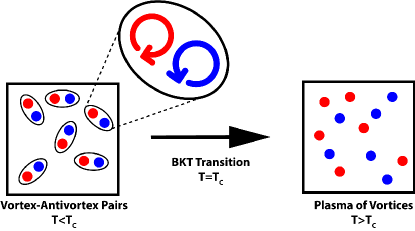
Figure 1: Vortex binding and unbinding on the two side of the BKT transition. Figure taken from Giedt and Flamino (2018).

In this article we will study the sine-Gordon model. It is the effective theory of the vortices in the XY model, and has the Euclidean action:

$$S[\phi]=\frac{1}{t}\int d^{2}x~{}\left\{\frac{1}{2}[{\partial}_{\mu}\phi(x)]^{2}-g\cos\phi(x)\right\}$$ (1)

Here, $t$ is the “stiffness.” Interestingly, it corresponds to the inverse temperature of the corresponding XY model. The quantity $y=g/2t$ is the fugacity of vortices. The small $g$, or small $y$, behavior of the sine-Gordon theory is well understood. For $t>8\pi$ (the low temperature regime of the XY model), the renormalization group (RG) flow (toward the infrared) of $g$ is $g\to 0$. We thus recover the theory with long range correlations (algebraic ordering) in this part of the phase diagram. By contrast, for $t<8\pi$ (the high temperature regime of the XY model), the flow of $g$ is $g\to\infty$, which leads to screening and an absence of criticality.

Since $t>8\pi$ corresponds to the low temperature phase of the XY model, this is where the line of fixed points will occur. It is here that one has continuously varying critical exponents, and conformal field theories will describe the infrared physics. Since this is a two-dimensional theory, the conformal group is infinite dimensional, with generators $L_{m}$ satisfying the well-known Virasoro algebra. Note that this infinite dimensional symmetry algebra emerges at long distances, associated with the flow $y\to 0$ of the renormalization group. Thus it is challenging to obtain the composite field operators of the ultraviolet theory that will correspond to the Virasoro generators. This is because the conformal symmetry is not a feature of the ultraviolet theory, due to the nonzero $y$.

As mentioned above, the temperature $t$ of the sine-Gordon theory maps to an inverse temperature in the XY model. In the XY model, the correlation length $\xi$ approaches criticality according to $\xi\sim e^{a/\sqrt{t_{\text{red}}}}$, where $t_{\text{red}}=(T-T_{\text{BKT}})/T_{\text{BKT}}$ is the reduced temperature. In the sine-Gordon theory this becomes $\xi\sim e^{b/\sqrt{8\pi-t}}$ for $t<8\pi$, where $\xi$ is the correlation length. Thus we continue to have an essential singularity in the critical temperature/stiffness. A result of this is that the transition is of infinite order, so that derivatives of the free energy will be smooth functions. We find results consistent with this in our study of the entropy below, in Section VI.

The sine-Gordon model belongs to the family of solid-on-solid (SOS) models which have critical behavior consistent with the BKT transition. When one looks into the origin of the SOS models, one finds a roughening transition. The correspondence between roughening transitions in crystal facets and the XY universality class was first discussed in Chui and Weeks (1976, 1978). The variable $\phi(x)$ of the sine-Gordon model is interpreted as a height variable above a two-dimensional (2d) surface—the facet of a crystal. Below, we display figures that visualize this picture from actual simulations; see Figs. 20 and 21. As a result, above the critical $t$, where $\phi(x)$ becomes highly nonuniform, the sine-Gordon model describes the high temperature growth of a rough surface. There is a critical line $t_{c}(y)$, and the fugacity $y$ labels different types of crystals. When $y\gg 1$, the cosine potential term in the action (1) dominates and one is driven to the uniform ground states where $\phi(x)$ is frozen to a multiple of $2\pi$. Thus we expect the curve $t_{c}(y)$ to tend to infinity as $y$ is increased, as shown in the sketch, Fig. 2.

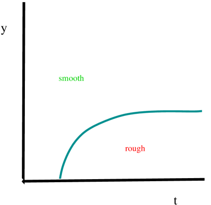
Figure 2: Sketch of hypothetical phase boundary for sine-Gordon model.

It was mentioned above that the sine-Gordon theory is a toy model for ${\cal N}=4$ super-Yang-Mills because it has a line of fixed points where nontrivial conformal field theories exist. There is an additional correspondence, namely the duality between solitons and elementary excitations. In the present case, the sine-Gordon theory is known to be dual to the massive Thirring model, with kink-like solitons in the sine-Gordon theory being dual to elementary fermions in the Thirring theory Coleman (1975). A similar duality exists in ${\cal N}=4$ super-Yang-Mills: on the Coulomb branch, W-bosons are dual to ’t Hooft-Polyakov monopoles, which are type of soliton. Thus by studying duality on the lattice in the context of the sine-Gordon model and Thirring model, we can lay groundwork for the eventual study of electric-magnetic S-duality in ${\cal N}=4$ super-Yang-Mills. This has a practical advantage in that simulating two-dimensional models is far less costly in terms of computer resources.

In this article we explore the behavior of two useful observables in a lattice formulation of the sine-Gordon model. We use the method of Fourier accelerated hybrid Monte Carlo, discussed in the next section. We are able to identify the value of $t$ where the topological transition occurs, and find that it agrees with previous determinations. We also provide some evidence that the transition is of infinite order. Preliminary aspects of a part of this study have previously appeared in Giedt and Flamino (2018).

We now summarize the content of this article. In Section II we review Fourier acceleration of hybrid Monte Carlo. In Section III we review the relation between the 2d Coulomb gas and the sine-Gordon model, which also allows us to exhibit the fugacity expansion. This is relevant to various statements in later parts of the paper. In Section IV a few words about the solitons of this model are given. These are again well-known facts. After this we move on to our results, beginning in Section V where we show our main simulation results and the thickness observable. We find results consistent with those obtained in an earlier study by Hasenbusch et al. Hasenbusch et al. (1994), which used a cluster algorithm. Next in Section VI we show our explorations of entropy, and find a picture that is consistent with an infinite order transition. Section VII takes a closer look at the domains that form when the barrier height is significant. We close the paper with Conclusions and a number of Appendices that review some details related to earlier discussion, including finer points of well-known results. The appendices also discuss some of the technical points of our implementation, and general musings about the fugacity expansion.

II Fourier acceleration

In this section we briefly discuss the Fourier accelerated hybrid Monte Carlo (HMC) algorithm that is the basis of our simulations Duane et al. (1985); Ferreira and Toral (1993). The point this generalization of HMC is to reduce autocorrelations between configurations of $\phi(x)$ that are produced in the course of the simulation. Provided this is successful, a shorter simulation can be used, while producing equivalent results and uncertainties. Previous work using Fourier accelerated HMC includes Espriu et al. (1997); Catterall and Karamov (2002).

At the beginning of the HMC simulation, the momentum field $\pi(x)$ is drawn at random from a Gaussian distribution with unit variance. This corresponds to “integrating in” a Gaussian field in the partition function, leading to the “Hamilitonian”

$$H=\sum_{x}\bigg{\{}\frac{1}{2}\pi^{2}(x)-\frac{1}{2t}\phi(x)\Delta\phi(x)-\frac{g}{t}\cos\phi(x)\bigg{\}}$$ (2)

where as usual the Laplacian is discretized by

$$\Delta\phi(x)=\sum_{\mu=1}^{2}{\partial}_{\mu}^{*}{\partial}_{\mu}\phi(x)=\sum_{\mu=1}^{2}\left[\phi(x+{\hat{\mu}})+\phi(x-{\hat{\mu}})-2\phi(x)\right]$$ (3)

Here, ${\partial}_{\mu}$ is the forward difference operator in the $\mu$ direction, ${\partial}_{\mu}^{*}$ is the backward difference operator, and ${\hat{\mu}}$ is a unit vector in the $\mu$ direction. As usual, we work in lattice units, $a=1$. The Hamiltonian $H$ is evaluated to obtain $H(0)$. Next, the fields $\pi(x),\phi(x)$ are evolved according to Hamilton’s equations

$$\dot{\phi}(x)=\frac{{\partial}H}{{\partial}\pi(x)},\quad\dot{\pi}(x)=-\frac{{\partial}H}{{\partial}\phi(x)}$$ (4)

for a trajectory of length $\tau$, which we typically set to 1. The numerical integration technique for this evolution in fictitious time should be reversible and area-preserving, where area refers to the functional integration measure $[d\pi(x)~{}d\phi(x)]$. The standard method is the leapfrog algorithm, which is what we use. This integrator has step size $dt$, and the Hamiltonian $H(\tau)$ at the end of the leapfrog trajectory will differ from $H(0)$ due to $dt$ not being zero. To correct for this, we apply the Metropolis accept/reject step

$$P_{\text{acc}}=\min(1,e^{-\Delta H}),\quad\Delta H=H(\tau)-H(0)$$ (5)

to obtain a “perfect” algorithm, which will sample the functional integral with the correct weight, the canonical distribution corresponding to $H[\pi(x),\phi(x)]$.

The Fourier acceleration is introduced into the leapfrog trajectory, where the Fourier modes of $\phi(x)$ and $\pi(x)$ are integrated with a step size

$$dt(k)=dt/(\Delta(k)+m_{\text{eff}}^{2})$$ (6)

An equal number of steps $N_{\tau}=\tau/dt$ are taken for each mode $k$. The Fourier transform of the force $-{\partial}H/{\partial}\phi(x)$ must also be used in these equations. In (6), $\Delta(k)$ is the Fourier transform of $-\Delta(x,y)$:

$$\Delta(k)=\sum_{\mu=1}^{2}4\sin^{2}(\pi k_{\mu}/L_{\mu}),\quad k_{\mu}=0,\ldots,L_{\mu}-1$$ (7)

for an $L_{1}\times L_{2}$ lattice. By evolving the longer wavelength modes with a larger step size, they are moved farther in configuration space. This tends to reduce autocorrelations, because it is precisely the long wavelength modes that lead to long autocorrelation times.

It is certainly not necessary to take the $k$ dependent step size $dt(k)$ to be of the form (6). A further study that we will conduct at a future point is to generalize the choice of $dt(k)$ and then optimize it using machine learning techniques. The figure of merit that will be maximized (i.e., the training goal) is the inverse of the integrated autocorrelation time. Our current study that has the feature of being a first step in extensive investigations of the Fourier acceleration technique, using the sine-Gordon model as easily simulated toy model.

III Relation to the two-dimensional Coulomb gas

An important property of the SG model is its relation to the 2d Coulomb gas. It is here that one can understand its dynamics in terms of a collection of charges. Concrete applications include the physics of defects in liquid crystals, vortices in superconducting thin films, and vortices in 2d superfluids, such as a monolayer of ⁴He on a substrate. Such features can also be realized in cold atom arrays. It is worth noting that some of the most important properties of BKT physics can be obtained from the multiple perspectives. For instance the renormalization group equations that were originally obtained by Kosterlitz Kosterlitz (1974) can also be obtained from the sine-Gordon model Amit et al. (1980).

The correlation functions that are the focus of this aspect of the sine-Gordon model are not those of the elementary fields $\phi(x)$. Rather, we work with what high energy physicists would call “composite operators,” $e^{\pm i\phi(x)}$. These have an interpretation as vortex and antivortex creation operators.

III.1 Two-point function

The basic two-point function to be considered is

$$G(x-y)=\langle e^{i\phi(x)}e^{-i\phi(y)}\rangle$$ (8)

which corresponds to the amplitude for the creation of a vortex at $y$ and its subsequent annihilation at $x$. The action that determines this amplitude in the path integral has been given above in Eq. (1), leading us to evaluate

$$G(x)=Z^{-1}\int[d\phi(z)]e^{-S_{0}(\phi)}e^{i[\phi(x)-\phi(0)]}e^{(g/t)\int d^{2}y\cos\phi(y)}$$

$$Z=\int[d\phi(z)]e^{-S_{0}(\phi)}e^{(g/t)\int d^{2}y\cos\phi(y)}$$

$$S_{0}(\phi)=\frac{1}{2t}\int d^{2}x~{}[{\partial}_{\mu}\phi(x)]^{2}$$ (9)

We proceed by expanding the exponential

$$e^{(g/t)\int d^{2}y\cos\phi(y)}$$

in powers of $g/t$:

$$\sum_{n=0}^{\infty}\frac{1}{n!}\left((g/t)\int d^{2}y~{}\cos\phi(y)\right)^{n}=1+\frac{g}{2t}\int d^{2}y~{}\left(e^{i\phi(y)}+e^{-i\phi(y)}\right)$$

$$+\frac{g^{2}}{8t^{2}}\int d^{2}y_{1}~{}d^{2}y_{2}~{}\big{(}e^{i[\phi(y_{1})+\phi(y_{2})]}+e^{-i[\phi(y_{1})+\phi(y_{2})]}$$

$$+e^{i[\phi(y_{1})-\phi(y_{2})]}+e^{-i[\phi(y_{1})-\phi(y_{2})]}\big{)}+\ldots$$ (10)

In the correlation function, only the terms with an equal number of plus signs and minus signs in the exponent will survive. This further implies that only even powers of $g$ will contribute ($n$ even). The interpretation of the $n$th term in this sum

$$\prod_{i=1}^{n}e^{i{\epsilon}_{i}\phi(y_{i})},\quad{\epsilon}_{i}=\pm 1,\quad\sum_{i=1}^{n}{\epsilon}_{i}=0,\quad n\in 2{\bf Z}$$ (11)

is the virtual pair production of $n/2$ vortex-antivortex pairs that interact with the vortex at $y$ and antivortex at $x$ as well as with each other. The connection between the 2d Coulomb gas, the interpretation in terms of vortices of the XY model, and the sine-Gordon model has been explained in many places; see for instance Samuel (1978); Benfatto et al. (2013); Zinn-Justin (2002); Mudry (2014). One thing that is interesting is that the temperature $t$ of the sine-Gordon (roughening) model maps to an inverse temperature in the corresponding 2d Coulomb gas model. Hence there is a sort of $t\to 1/t$ duality between these equivalent descriptions, reminiscent of the Kramers-Wannier duality in the 2d Ising system or the strong-weak coupling duality $g\to 1/g$ (S-duality) in ${\cal N}=4$ super-Yang-Mills. Renormalizing the composite operators

$$e^{i{\epsilon}_{i}\theta(x)}=\zeta\left[e^{i{\epsilon}_{i}\theta(x)}\right]_{\text{ren.}},\quad\zeta=(\Lambda/\mu)^{-t/4\pi}$$ (12)

we obtain renormalized averages of these operators in the theory with action $S_{0}$ (i.e., the free theory)

$$\left\langle\prod_{i=1}^{n}e^{i{\epsilon}_{i}\phi(x_{i})}\right\rangle_{\text{ren.}}=\prod_{i<j}(\mu|x_{i}-x_{j}|)^{{\epsilon}_{i}{\epsilon}_{j}t/2\pi}$$ (13)

From this we find that

$$\left\langle e^{i[\phi(y)-\phi(z)]}\right\rangle_{\text{SG}}$$

$$=Z_{\text{SG}}^{-1}\sum_{n\in 2{\bf Z}}\frac{g^{n}}{2^{n}t^{n}n!}\int d^{2}x_{1}\cdots d^{2}x_{n}\sum^{\prime}_{\{{\epsilon}\}}\prod_{i<j}(\mu|x_{i}-x_{j}|)^{{\epsilon}_{i}{\epsilon}_{j}t/2\pi}$$ (14)

Here $i,j=0,\ldots,n+1$ with $x_{0}=y$, $x_{n+1}=z$ and ${\epsilon}_{0}=1$, ${\epsilon}_{n+1}=-1$ so that they are not summed over, hence the primed summation symbol. $Z_{\text{SG}}$ is the same expression but without the $i,j=0$ and $n+1$ terms (vacuum diagrams only). I.e.,

$$Z_{\text{SG}}=\sum_{n}\frac{g^{n}}{2^{n}t^{n}n!}\int d^{2}x_{1}\cdots d^{2}x_{n}\sum_{\{{\epsilon}\}}\prod_{i<j}(\mu|x_{i}-x_{j}|)^{{\epsilon}_{i}{\epsilon}_{j}t/2\pi}$$ (15)

with $i,j=1,\ldots,n$ only.

Note that there are singularities when ${\epsilon}_{i}{\epsilon}_{j}<0$ and $x_{i}\to x_{j}$ under the integration. It is not an integrable singularity for $t\geq 4\pi$. So it is not the case that we have rendered the correlation function finite to all orders simply by renormalizing the composite fields by the factor $\zeta$. All that has been accomplished is to make (13) finite, but the subsequent integration of this expression in the sine-Gordon model leads to further difficulties. This is one reason to perform the lattice discretization, because all quantities are under control and finite.

Hard-core repulsion can be inserted into the above formula, thereby avoiding $x_{i}=x_{j}$. Of course, this does not follow from the path integral of the sine-Gordon model directly, but is an add-on to control the singularity and model the regulation of this infinity in the physical system. The long distance singularity that occurs from infinite $|x_{i}-x_{j}|$ can also be moderated by periodic boundary conditions or some other finite system size regulation, which is again a matter of inserting physical constraints on the mathematical calculation in order to avoid the bad behavior.

III.2 Observations about renormalization

It may be that we would like to renormalize the theory, absorbing the UV divergences in the low energy parameters. To accomplish this in renormalized perturbation theory, we would cancel these infinities with counterterms; or, equivalently, we would rescale the bare fields and re-express the bare parameters in terms of long distance quantities. The problem is whether redefinitions of $t$ and $g$, together with $\phi\to\sqrt{Z}\phi$, suffices. After all, classically, the mass dimension of $\phi$ is $d_{\phi}=\frac{1}{2}(d-2)=0$, so we can write down an infinite number of counterterms in the renormalizable Lagrangian. The potential $(g/t)\cos(\phi(x))$ is not unique according to this power-counting based around the Gaussian fixed point. However, the field $\phi(x)$ will acquire an anomalous mass dimension, as will operators built upon it; so we expect that only a finite number of operators will be relevant or marginal once quantum effects are taken into account. Certainly the observed universality of XY type models suggests this.

One constraint on the renormalized theory is the invariance of the bare theory under the shift symmetry $\phi(x)\to\phi(x)+2\pi$. Certainly this forbids a host of terms in the potential. However, it allows for terms of the form $\cos[p\phi(x)+\alpha]$ where $p$ is any integer and $\alpha$ is a real number.

The way that we would normally proceed is to enumerate all of the one-particle irreducible (1PI) functions and vertex functions that have a non-negative superficial degrees of divergence. That would tell us how many counterterms we need. But since we are working in position space (due to the composite operators and cosine potential) and have integrals over $x$, it is not clear how to do the counting in a perturbation theory structured around the fugacity expansion. Also, this is in terms of composite fields, and we are not working with vertices of elementary fields. In fact, the casual observer will not immediately see a diagramatic expansion in the above formula. So the usual tools seem to be off the table. We will address this conundrum in analysis that follows.

From the work of Halperin and Nelson (1979a) we know that in superconducting thin films, the behavior can be modeled as a superposition of BKT fluctuations and Ginzburg-Landau (GL) fluctuations. In our sine-Gordon model we will be spared of this complication, because it only describes the vortex dynamics of the XY model. However it is interesting to think about how this feature might be incorportated into the effective field theory, and we will have some further comments on this direction of research in the conclusions.

IV Solitons

The minima of the potential $V(\theta)$ occur at

$$\phi(x)=2\pi n,\quad n\in{\bf Z}$$ (16)

The solitons occur for static configurations

$$\frac{{\partial}\phi(t,x)}{{\partial}t}=0$$ (17)

Hence $\phi(t,x)=\vartheta(x)$. The topologically nontrivial solitons asymptote to different vacua:

$$\lim_{x\to-\infty}\vartheta(x)\to 2\pi n_{-},\quad\lim_{x\to\infty}\vartheta(x)\to 2\pi n_{+},\quad n_{-}\not=n_{+}$$ (18)

We are particularly interested in the configurations that are minima of the configuration energy

$$E=\frac{1}{t}\int_{-\infty}^{\infty}dx~{}\left\{\frac{1}{2}({\partial}_{x}\vartheta)^{2}+V(\vartheta)\right\}$$ (19)

subject to the boundary conditions (18). These are solutions to the static equations of motion (saddle point equation in this Euclidean formulation)

$$\frac{\delta E}{\delta\vartheta(x)}=0\quad\Rightarrow\quad{\partial}_{x}^{2}\vartheta=\frac{{\partial}V}{{\partial}\vartheta}$$ (20)

The solutions are well known; they are given for instance in the wonderful review of topological solitons by ’t Hooft, Chapter 4.1 of ’t Hooft (1994). For instance, in the case of $n_{-}=0$ and $n_{+}=1$, the soliton is described by the first branch of

$$\vartheta(x)=4\arctan e^{mx},\quad m^{2}=\frac{g}{t}$$ (21)

Of course in our dynamical configurations this will not be exactly true (until we cool), and so we would like to have a way of measuring the mass $m_{\text{eff}}$ of the soliton from such non-extremal configurations. We will explore this in future work.

On the lattice we have an $S^{1}\times S^{1}$ geometry, so the asymptotic behavior described above does not make sense. However, we can still have nontrivial topology by incorporating twisted boundary conditions in the spatial direction $x=x_{1}$:

$$\theta(t,x+N_{x}a)=\theta(t,x)+2\pi n,\quad n\in{\bf Z}$$ (22)

This is also left to future work.

V Simulation results

As we approach the transition temperature, an increasing number of degrees of freedom participate in the low energy theory, as can be seen by the onset of “algebraic ordering,” corresponding to a divergent correlation length. This makes the fugacity expansion unreliable, and in fact is the reason that renormalization group methods were employed to understand the transition. We therefore turn to a numerical study of the model where all features are regulated by the lattice’s UV and IR cutoffs.

V.1 $\phi$ distribution and vacuum degeneracy

As we have seen in the previous section, the form of the potential $V(\phi)\sim\cos(\phi)$ indicates that there will be an infinity of degenerate vacua, $\phi\sim 2\pi n$, $n\in\mathbb{Z}$. We expect to see this feature in the simulations, although the tunneling reflects the algorithm in addition to the physical barrier between these vacua. In Fig. 3 we show the history of the average

$$\phi_{\text{avg}}=\frac{1}{V}\sum_{x}\phi(x)$$ (23)

where $V=L_{0}L_{1}$ is the simulation volume. Time along the bottom axis is the simulation time, measured in molecular dynamics time units (MDTU). It can be seen that for $t=1.0$ and $g=2.0$ (fugacity of $y=1.0$), no tunneling between the various vacua occurs; here, the simulation was initiated at $\phi=0$. Clearly the barrier is too large to allow HMC to move into other vacua. In Fig. 4 we reduce the barrier ten-fold, setting $g=0.2$ (fugacity of $y=0.1$), and now there is significant migration between the vacua. Of course since the barrier height is inversely proportional to $t$, the effective tunneling rate will also depend on this quantity. In Fig. 5 we show what occurs for three different values of $t$, all with $g=0.4$. As per expectations, tunneling is significantly suppressed by decreasing $t$. Fig. 6 shows a much larger lattice, $64\times 64$ ($L=64$), where it is possible that domains are forming, consisting of the different vacua. In this case the different vacuum values of $\phi$ would tend to cancel, giving a result that fluctuates about zero. It can be seen in Fig. 7 that domains have not formed, but rather on the larger lattice it is simply stuck near the $\phi=0$ vacuum, rather than tunneling. Apparently, on the larger volumes, tunneling is more difficult due to a tendency toward coherence across the entire lattice.

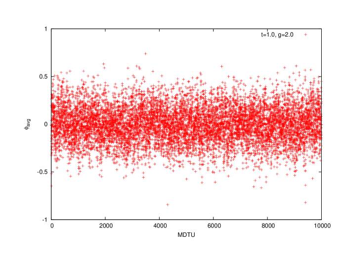
Figure 3: The average value of $\phi$ on a $4\times 4$ lattice as a function of simulation time, for $t=1.0$ and $g=2.0$. It can be seen that the field fluctuates about the vacuum it was started in, $\phi(x)=0\;\forall\;x$. The barrier to tunneling to other vacua is too great for the HMC to allow it.

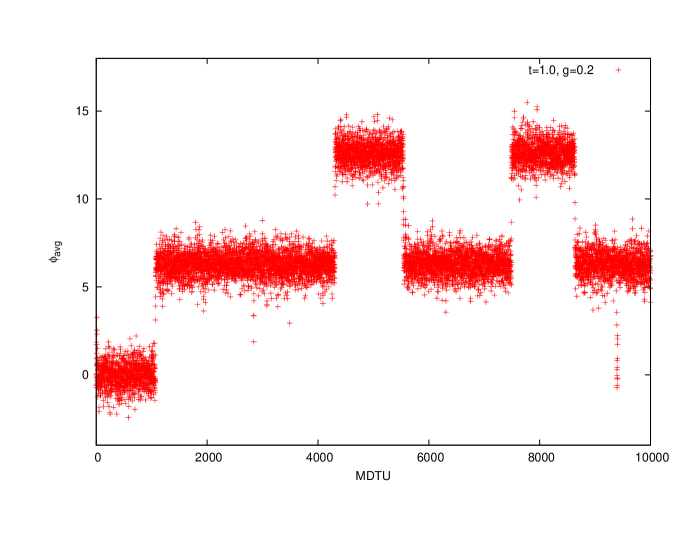
Figure 4: The average value of $\phi$ on a $4\times 4$ lattice as a function of simulation time, for $t=1.0$ and $g=0.2$. I.e., a barrier height 10 times lower than in Fig. 3. It can be seen that the field now tunnels between vacua $\phi(x)=2\pi n\;\forall\;x$, $n\in\mathbb{Z}$. With $g=0.2$, the barrier to tunneling to other vacua is low enough for the Fourier accelerated HMC to allow it. Because the lattice is small, the entire field configuration moves coherently between the vacua.

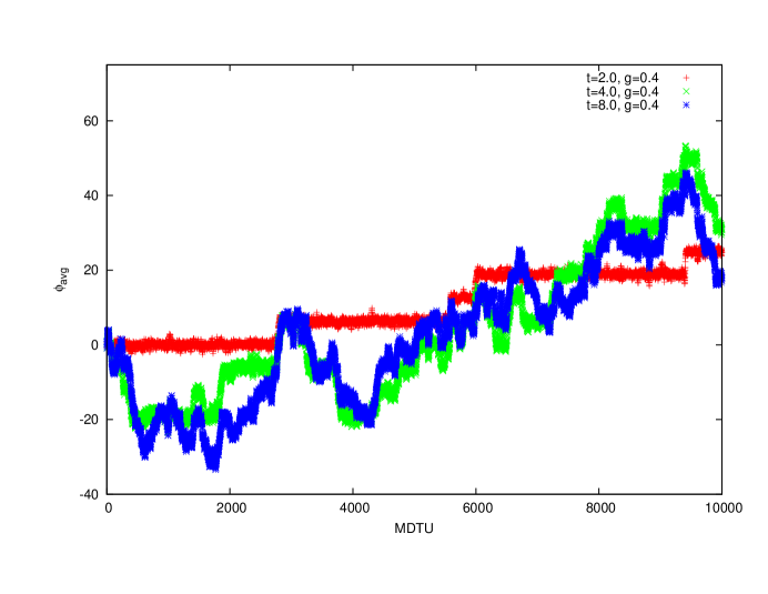
Figure 5: The average value of $\phi$ on a $4\times 4$ lattice as a function of simulation time, for three different values of $t$ and $g=0.4$. It can be seen that at smaller $t$ the field rarely tunnels between vacua $\phi(x)=2\pi n\;\forall\;x$, $n\in\mathbb{Z}$, whereas for larger $t$ the tunneling is fairly rapid. This is because the height of the barrier is proportional to $1/t$ and the strength of fluctuations is proportional to $\sqrt{t}$.

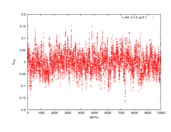
Figure 6: The average value of $\phi$ on a $64\times 64$ lattice as a function of simulation time. Although the couplings are the same as in Fig. 4, the lattice has 256 times more sites, opening up the possibility of forming domains of the different vacua. If that was the case, they would tend to cancel in the average of $\phi$, leading to values close to zero. Thus a finer-grained study of the lattice configurations is necessary in order to resolve what is going on. In fact, Fig. 7 shows that this is not what is occuring. Rather, the entire lattice collapses almost immediately into a single domain, and remains there, in contrast to what happens on the $4\times 4$ volume of Fig. 4.

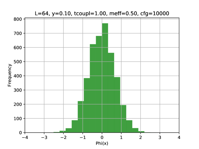
Figure 7: Histogram of the $\phi$ value for a simulation with lattice size $L=64$, temperature $t=1.0$, coupling $g=0.2$ ($y=0.1$), for configuration number 10,000 in the simulation, showing that it is centered around one vacuum config, and not really forming domains. This answers the question that was raised in the caption of Fig. 6.

V.2 Thickness

In Hasenbusch et al. (1994), Hasenbusch et al. introduce the thickness:

$${\sigma}^{2}=\frac{1}{V^{2}}\sum_{x,y}{\langle(\phi(x)-\phi(y))^{2}\rangle}$$ (24)

In this formula, $V=L\times L$ is the system size, “volume.” They show that this is a useful observable for identifying the critical regime. We will use it here, and find results consistent with theirs. The thickness is a measure of the roughness, on average, for a given parameter pair $(t,y)$. For example, if the entire lattice sits in a single domain, with small fluctuations, then ${\sigma}$ will be small. However, domain walls will contribute a nonzero result even in the absence of fluctuations, so ground state disorder will increase the thickness observable.

In order to not bias toward a particular ground state, unless otherwise stated we begin all of our simulations in studies of thickness with a random start, as in Fig. 8, which has $\phi\in[-20,20]$ uniformly distributed.

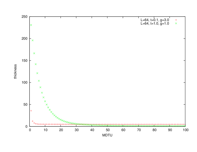
Figure 8: The thickness on a $64\times 64$ for two different choices of $t$ and $g$, as function of simulation time, beginning with the random start described in the text. For the case of a steep potential, $y=g/2t=15$, the fields rapidly settle into minima and the thickness becomes small, as it only gets contributions from domain walls between the minima. Note however, that ultimately the thickness is largers because that corresponds to small $t=0.1$, whereas the $t=1.0$ data has much larger fluctuations. This is because the first term in the action, the kinetic term, is the one that determines the size of fluctuations about any given classical vacuum.

Before taking averages and estimating uncertainties, one should study and characterize the autocorrelation of the thickness observable. This is because we need several autocorrelation times in order to thermalize, and we need to know the separation between statistically independent samples—where the Monte Carlo simulation is effectively a Markov process. The autocorrelation for any observable ${\cal O}(t)$, where $t$ here is the simulation time (measured in MDTUs), is given by

$$C(t) = \frac{1}{{\cal N}}\frac{1}{N-t}\sum_{t^{\prime}=0}^{N-t-1}({\cal O}(t^{\prime}+t)-{\langle{\cal O}\rangle})({\cal O}(t^{\prime})-{\langle{\cal O}\rangle})$$

$${\cal N} = \frac{1}{N}\sum_{t=0}^{N-1}({\cal O}(t)-{\langle{\cal O}\rangle})^{2},\quad{\langle{\cal O}\rangle}=\frac{1}{N}\sum_{t=0}^{N-1}{\cal O}(t)$$ (25)

and $N$ is the total number of time steps in the simulation, $t=0,1,\ldots,N-1$. In the present case,

$${\cal O}=\frac{1}{V^{2}}\sum_{x,y}(\phi(x)-\phi(y))^{2}$$ (26)

In Figs. 9, 10 and 11 we show short, long and very long time scales. It can be seen that there is an initial rapid decay, but that a longer time component also contributes. In fact it takes ${{\cal O}(10^{3})}$ or more updates to obtain a completely independent configuration. These results are for $y=0.1$ with $t$ values that bracket what will turn out to be the critical temperature, $t_{c}\approx 18$. In fact, it can be seen that $t\approx t_{c}$ yields the longest autocorrelation times, which is to be expected. This is because critical fluctuations, which have very long wavelength, lead to significant slow-down in typical Monte Carlo algorithms. We see that the Fourier acceleration has not been entirely effective in alleviating this critical slowing down. Amusingly, monitoring the autocorrelation can be a surprisingly good way to locate the critical temperature.

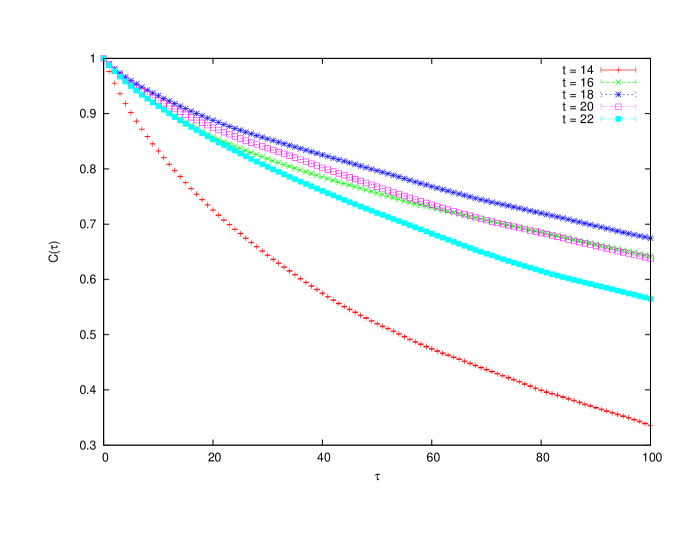
Figure 9: The autocorrelation in the thickness observable on a $64\times 64$ lattice for $y=0.1$, and $t$ that bracket the phase transition. This figure shows short time scales, with accompanying figures showing longer time scales. It can be seen that for $t\approx t_{c}\approx 18$, the autocorrelation is the greatest, as is to be expected. Figure previously appeared in Giedt and Flamino (2018).

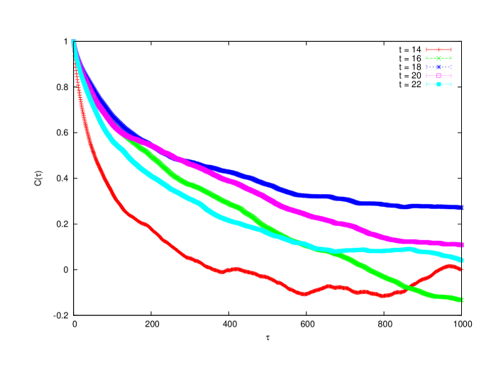
Figure 10: The autocorrelation in the thickness observable, showing longer time scales than Fig. 9. It can be seen that even after 1,000 updates, autocorrelations are still significant for temperatures close to the critical temperature of $t_{c}\approx 18$. Figure previously appeared in Giedt and Flamino (2018).

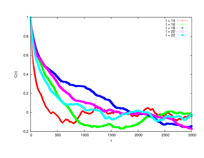
Figure 11: The autocorrelation in the thickness observable, showing very long time scales, compared to Figs. 9 and 10. It can be seen that by ${{\cal O}(3000)}$ time steps all memory of the initial configuration has vanished. Figure previously appeared in Giedt and Flamino (2018).

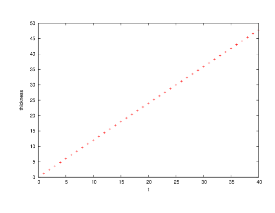
Figure 12: Thickness versus $t$ for $y=0.1$ for an $L=32$ lattice. It can be seen that it is a linear function of $t$ for this relatively weak value of $y$.

As will be seen in subsequent figures, a more interesting behavior occurs for $y>1$.

We next turn to results where we hold the fugacity $y=g/2t$ fixed as we vary $t$. In Fig. 12 we show the thickness for $y=0.1$, which is near the IR fixed point where $y=0$. It can be seen that for these small $t$ values, and at small $y$, the thickness just behaves as a Gaussian variance directly proportional to $t$. It thus appears that the $y$ coupling has essentially no effect in this regime, other than to determine the slope of the line. A further ellaboration of the behavior of the thickness as a function of $t$ and $y$ is given in Figs. 13 and 14.

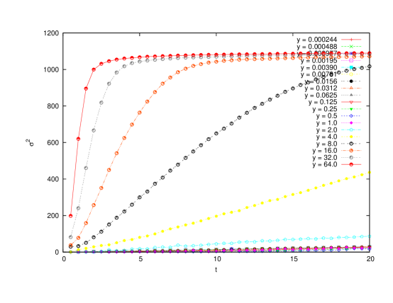
Figure 13: Thickness versus $t$ for various $y$ for an $L=64$ lattice. It can be seen that a cross-over between different behaviors occurs for $y\sim 1$, with a nonlinear dependence of ${\sigma}^{2}$ on $t$ appearing for large $y$.

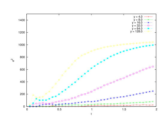
Figure 14: Thickness versus $t$, at rather small $t$, for various $y$ for an $L=64$ lattice. Some interesting features emerge at the smallest values of $t$ seen in this resolution. It can be seen that the steep rise that was observed in the previous plot simply becomes steeper, with its center moving to smaller $t$, as $y$ increases.

In Fig. 15 we see that the approximately linear behavior ${\sigma}^{2}\sim t$ has a slope that rises with $L$, if $t$ is greater than some critical value. In fact it is this transition that will be used to identify our critical temperature in the finite size scaling analysis.

Hasenbusch et al. provide a perturbative prediction for the finite size scaling of the thickness above and below the transition temperature Hasenbusch et al. (1994). In our conventions it is given by

$${\sigma}^{2}\simeq\left\{\begin{array}[]{cc}\frac{t}{\pi}\ln L+\text{const.},&\quad t>t_{c}\\ \text{const.}&\quad t<t_{c}\end{array}\right.$$ (29)

in the large $L$ limit. They have also verified this behavior in Monte Carlo simulations using a cluster algorithm. We conduct the same study, but with the Fourier accelerated HMC. Fig. 16 shows precisely this behavior, with $t_{c}\approx 18$. We note that the $y\to 0$ limit (fugacity expansion) predicts $t_{c}=8\pi\approx 25$, so there is apparently some renormalization of $t$ arising from $y=0.1$. If we fit the coefficient $c$ of ${\sigma}^{2}\simeq c\ln L+\text{const.}$ for the $t=22$ data, we obtain $c\approx 6.7\pm 0.2$, which is to be compared with $t/\pi=7.0$. We attribute the small discrepancy ($1.5{\sigma}$) to a possible underestimation of errors and a renormalization of $t$.

There is also an RG interpretation of these results. The dimension of the cosine operator in the action is $\Delta=t/4\pi$ (see for instance the discussion in Section 4.6 of Fradkin (2013)). Thus for $t>8\pi$, the cosine operator is irrelevant and the theory flows to a free theory, which will be ungapped and thus show the logarithmic divergence in the thickness variable. By contrast for the $t<8\pi$ case it will flow to a heavily gapped theory that cuts off sensitivity to the finite size, and thus gives a fixed result for the thickness as a function of $L$.

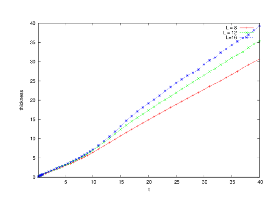
Figure 15: The thickness observable rises essentially linearly with $t$ for $y=0.1$. However, the slope increases with $L$, as can be seen from these low $L$ values. Note that this increase in slope only occurs in a noticeable way for $t$ greater than a critical value of around $10$. A more precise estimate of $t_{c}\approx 18$ will be obtained in our finite size scaling study below, summarized in Fig. 16.

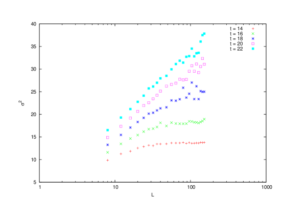
Figure 16: The thickness observable transitioning between the two behaviors (29) at $t_{c}\approx 18$. Here, we have used $y=0.1$.

VI Entropy

Another important observable is the entropy of the system for different values of the fugacity. The entropy ${\cal S}$ is calculated using

$${\cal S}=-\left(\frac{{\partial}F}{{\partial}t}\right)_{y},\quad F=-t\ln Z$$ (30)

We now show that

$${\cal S}(t)=\ln Z(t)+{\langle S(t)\rangle}$$ (31)

where $S(t)$ is the lattice action introduced above, which has an explicit factor of $1/t$. As a first step we therefore write

$$S(t)=\frac{1}{t}{\hat{S}}$$ (32)

where now ${\hat{S}}$ does not depend on $t$. It is then clear that

$${\cal S} = \ln Z+\frac{t}{Z}\frac{{\partial}}{{\partial}t}\int[d\phi]e^{-\frac{1}{t}{\hat{S}}}$$ (33)

$$= \ln Z+\frac{1}{Z}\int[d\phi]\frac{1}{t}{\hat{S}}e^{-S}$$

$$= \ln Z+{\langle S\rangle}$$

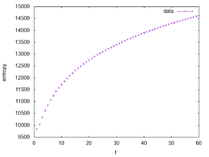
Figure 17: Entropy vs. temperature for fugacity $y=0.1$.

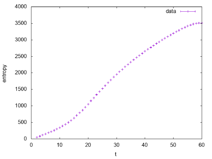
Figure 18: Entropy vs. temperature for fugacity $y=1$.

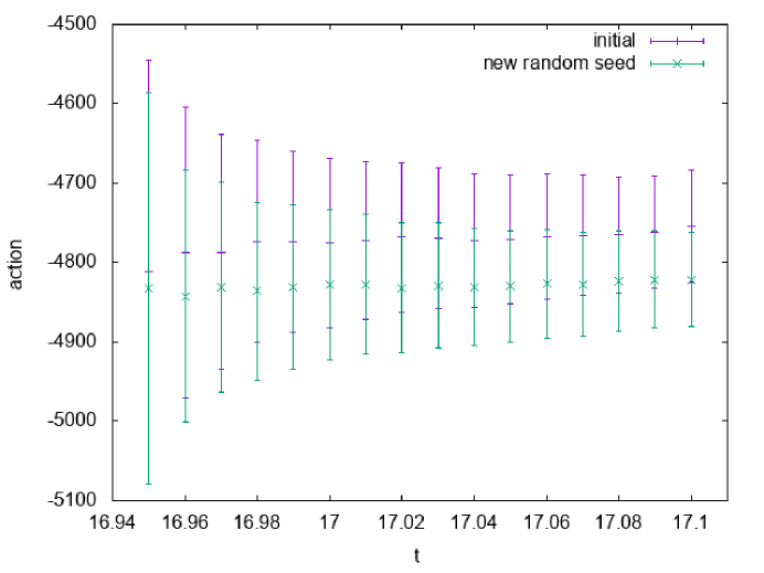
Figure 19: Average action vs. temperature for fugacity $y=1$.

Next we must discuss the computation of $\ln Z(t)$. With Monte Carlo sampling, we can only do this relative to some fixed value $Z(t_{0})$. Thus we use

$$\int_{t_{0}}^{t}\frac{d}{dt}~{}\ln Z(t)~{}dt=\ln\frac{Z(t)}{Z(t_{0})}$$ (34)

To find $d\ln Z(t)/dt$ we use the identity

$$\frac{d}{dt}\ln Z(t)=\frac{1}{t}{\langle S(t)\rangle}$$ (35)

from above. Thus, we can obtain $\ln[Z(t)/Z(t_{0})]$ from a straightforward expectation value—exactly what is easily calculated in the course of a Monte Carlo simulation.

For a select set of $t$, the action is calculated for 50,000 configurations, where the data starts to be recorded after 10,000 steps. This allows the system to thermalize. We perform this calculation for a wide range of $t$ and fit ${\langle S(t)\rangle}/t$ to a high order polynomial. The polynomial is then integrated to obtain $\ln[Z(t)/Z(t_{0})]$. For the reference value $t_{0}$, we choose $t_{0}=1$.

An example of the entropy analysis can be seen in Fig. 17 where entropy is calculated for a temperature range of $[0,60]$ for fugacity $y=0.1$. There appears to be a smooth logarithmic increase in entropy with respect to $t$. This makes sense, as a BKT transition is a transition of infinite order: a first derivative of the free energy is not expected to show a discontinuity, and in fact should be smooth. To confirm this expectation, in Fig. 18 another example is shown for a higher fugacity, $y=1$. Due to the higher potential barrier, tunneling was a lot more erratic across temperatures, so the action required a higher order polynomial to reliably model the free energy. And as can be seen in the figure, the resulting curve is smooth with a monotonically increasing entropy.

It is important to consider the effects of autocorrelation in this calculation of entropy as well. The observable is highly local, since it is a sum over the action density. The result is that the autocorrelation is significantly smaller than in the case of the thickness measurements, which involve correlations over large scales. In order to quantify this smaller autocorrelation, in Fig. 19 we show the action for $y=1$ generated for two separate random seeds, which alters the initialization of $\phi(x)$ at the beginning of the simulation. The difference between the action on the two sets of configurations is well within the error bars, which take into account integrated autocorrelation time in the usual way.

VII Clustering

We have analyzed the clustering of the field $\phi(x)$ into values around $2n\pi$, $n\in{\bf Z}$. The method for identifying a cluster is described in Appendix D. In Fig. 20 the various clusters found by this algorithm are shown from a perspective where they are all visible. Fig. 20 shows the same collection of clusters edge-on, where it is apparent that they are grouped into layers. In order to produce results with clearly defined domains, we found that it was helpful to use a random start with $\phi(x)$ drawn uniformly from $[-20,20]$ and a very large fugacity of $y=15$. We also set $t=0.1$ for this simulation, which tends to freeze the configuration into domains (very low temperature). The correlation between cluster “width” $W$ and population $P$ (the number of sites contained in the cluster) is show in Fig. 22, where 50 lattice configurations were combined. It shows an approximate behavior of

$$W\sim(\ln P)^{2}$$ (36)

Note that the largest population and width is limited by the fact that this is an $L=64$ lattice. We are not aware of a theoretical argument explaining the behavior (36), but leave it as a question for future investigations.

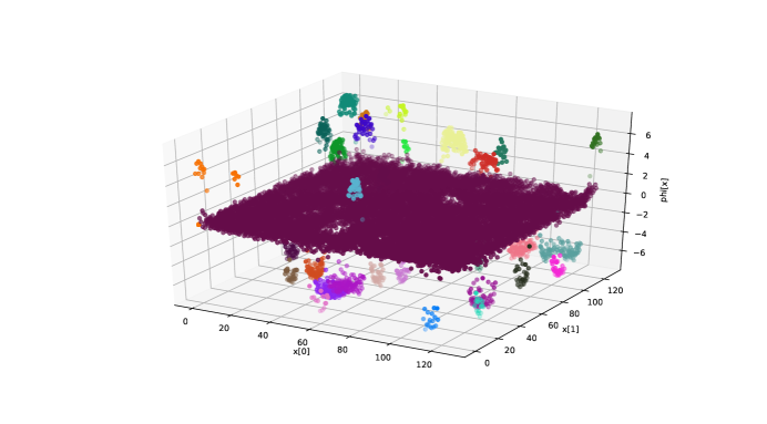
Figure 20: The clustering of the field $\phi(x)$ into domains for a particular (thermalized) configuration with $t=0.1$, $y=15$ and $L=64$. It can be seen that the bulk of the points cluster around $\phi=0$, but that other smaller clusters do form around the vacua at $\phi=\pm 2\pi$.

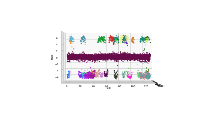
Figure 21: The same configuration as in Fig. 20, but from a different perspective.

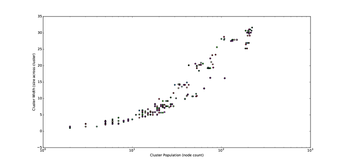
Figure 22: Correlation between cluster population and cluster “width.” The width of a cluster is the maximum size across in the two-dimensional domain. The population is the number of sites, or “nodes,” that have been identified as belonging to the cluster. Naturally the wider the cluster, the more nodes that it contains. However, the precise relationship is not so easily predicted, and empirically is logarithmic, according to Eq. (36).

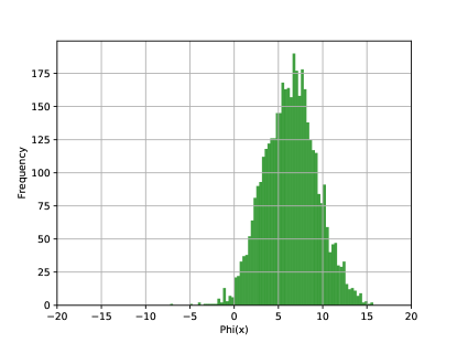
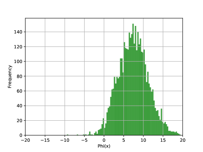
(a)	(b)
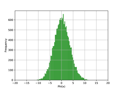
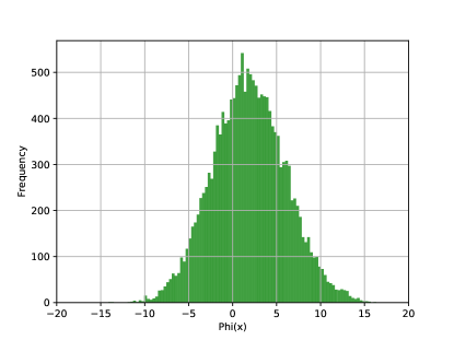
(c)	(d)

Figure 23: Distribution of field values on either side of the transition. Here, $L=64$ and $y=0.1$. Panel (a) is $t=14$ and panel (b) is $t=22$. These are the distributions for a single configuration, after 10000 thermalization updates. The two simulations were started from the same initial conditions with the same seed for the pseudorandom number generator, so that the differences are entirely due to the value of $t$. It can be seen that $t=22$ has longer tails, due to stronger fluctuations at the higher temperature. However, it is interesting that for this $L$, nothing dramatic occurs as we cross the transition. In (c) and (d) we show the same analysis for L=128.

VIII Conclusions

One interesting avenue to explore is the possible existence of three phases in the XY type systems, as shown in Fig. 24. Arguments for the existence of this more complicated set of transitions were advanced in classic papers by Halperin, Nelson and Young Halperin and Nelson (1978, 1979b); Young (1979); Nelson (1978). Although this feature has been argued for theoretically, and observed experimentally, it has still not been detected in numerical simulations to date. Thus, future work would be to use the more powerful and sophisticated simulation methods that are begun here to observe these types of behaviors. An important question is: “How would they be realized in the sine-Gordon model, if at all.” Does a theory of vortices contain enough information to capture the full dynamics of the XY model in this regard? We leave this question open to future research.

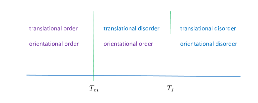
Figure 24: The three phases of algebraic order versus disorder, as advanced in the seminal papers of Halperin, Nelson and Young (1978-79).

We mentioned in the main body of the paper that in superconducting thin films one can understand the behavior as a superposition of BKT fluctuations (spin waves and vortices) and GL fluctuations. It would seem that the presence of GL fluctuations comes from the fact that the thin film is not truly two-dimensional, having a thickness $d$. This suggests an XY model with three dimensions, one of them being quite small. Alternatively, we could formulate a SG model built on layers. One would like to establish the connection between these ideas. Currently we are developing numerical simulations that will analyze such layered systems, especially in the limit of weak interlayer interactions.

Appendix A Free theory propagator

A.1 Continuum

We generalize the free action to include a mass term,

$$S_{0}(\theta)=\frac{1}{t}\int d^{2}x~{}\bigg{\{}\frac{1}{2}[{\partial}_{\mu}\phi(x)]^{2}+\frac{1}{2}m^{2}\phi^{2}(x)\bigg{\}}$$ (37)

We must include a mass term to regulate the infrared divergence. Then

$$\Delta(x,m)=\int\frac{d^{2}p}{(2\pi)^{2}}\frac{e^{ip\cdot x}}{p^{2}+m^{2}}$$ (38)

This can be evaluated with the help of results from Gradshteyn & Ryzhik (G&R) Gradshteyn and Ryzhik (1994). Passing to polar coordinates and using G&R 3.339 (p. 357)

$$\frac{1}{4\pi^{2}}\int_{0}^{\infty}\frac{pdp}{p^{2}+m^{2}}\int_{0}^{2\pi}d\theta~{}e^{ipx\cos\theta}=\frac{1}{2\pi}\int_{0}^{\infty}\frac{pdp}{p^{2}+m^{2}}J_{0}(px)$$ (39)

Then using G&R 6.532#4 (p. 702) we perform the integral obtaining

$$\frac{1}{2\pi}K_{0}(mx)$$ (40)

We are interested in the limit of small $m$, which is obtained from G&R 8.447 #3 & #1 (p. 971)

$$K_{0}(z)=-\ln\frac{z}{2}+\psi(1)+{{\cal O}(z)},\quad\psi(1)=-\gamma$$ (41)

Thus we finally obtain

$$\Delta(x,m)=-\frac{1}{2\pi}\ln\frac{mx}{2}-\frac{1}{2\pi}\gamma+{{\cal O}(m)}=-\frac{1}{4\pi}\left[\ln\frac{m^{2}x^{2}}{4}+2\gamma\right]+{{\cal O}(m)}$$ (42)

which agrees with ZJ (32.6) Zinn-Justin (2002).

Next we consider the correlation functions of composite operators as appears in (13), making use of (42) to prove this identity. The trick (e.g. Zinn-Justin (2002)) is to compute the path integral

$$\left\langle\prod_{i=1}^{n}e^{i{\epsilon}_{i}\phi(x_{i})}\right\rangle=Z_{0}^{-1}\int[d\phi(x)]e^{-S_{0}[\phi(x)]}\prod_{i=1}^{n}e^{i{\epsilon}_{i}\phi(x_{i})},\quad Z_{0}=\int[d\phi(x)]e^{-S_{0}[\phi(x)]}$$ (43)

by rewriting it in terms of a “source”

$$J(x)=i\sum_{i=1}^{n}{\epsilon}_{i}\delta(x-x_{i})$$ (44)

so that

$$\left\langle\prod_{i=1}^{n}e^{i{\epsilon}_{i}\phi(x_{i})}\right\rangle=$$

$$Z_{0}^{-1}\int[d\phi(x)]\exp\left(-\int d^{2}x~{}\left\{\frac{1}{2t}({\partial}_{\mu}\phi(x))^{2}+\frac{m^{2}}{2t}\phi^{2}(x)-J(x)\phi(x)\right\}\right)$$ (45)

This can be computed, as usual, by completing the square, leading to

$$\left\langle\prod_{i=1}^{n}e^{i{\epsilon}_{i}\phi(x_{i})}\right\rangle=\exp\left(\frac{t}{2}\int d^{2}x~{}d^{2}y~{}J(x)\Delta(x-y;m)J(y)\right)$$ (46)

Substituting (44) we obtain

$$\left\langle\prod_{i=1}^{n}e^{i{\epsilon}_{i}\phi(x_{i})}\right\rangle=\prod_{i,j=1}^{n}\left(\frac{m^{2}(x_{i}-x_{j})^{2}}{4}\right)^{\frac{t}{8\pi}{\epsilon}_{i}{\epsilon}_{j}}$$ (47)

To get closer to (13) we separate out factors

$$\lim_{\delta\to 0}\prod_{i}\left(\frac{m\delta}{2}\right)^{\frac{t}{4\pi}{\epsilon}_{i}^{2}}\cdot\prod_{i<j}\left(\frac{m|x_{i}-x_{j}|}{2}\right)^{\frac{t}{2\pi}{\epsilon}_{i}{\epsilon}_{j}}$$ (48)

where various factors of 2 have been accounted for in the exponents; in particular the double-counting of pairs in $\prod_{ij}$ versus $\prod_{i<j}$. The $\delta\to 0$ limit occurs because of the coincident “diagonal” terms $x_{i}=x_{j}$ in $\prod_{ij}$, and will in practice be regulated by lattice expressions for the propagator. I.e., they correspond to

$$\lim_{x_{i}\to x_{j}}\int_{-\pi}^{\pi}\frac{d^{2}k}{(2\pi)^{2}}\frac{e^{ik\cdot(x_{i}-x_{j})}}{{\hat{k}}^{2}+m^{2}}$$ (49)

where ${\hat{k}}_{\mu}=2\sin(k_{\mu}/2)$. Because of the compact domain of integration (finite lattice spacing), there is no singularity associated $x_{i}\to x_{j}$. The second factor of (48) agrees with (13), in terms of the dependence on $|x_{i}-x_{j}|$; everything else is swept into the renormalization factor $\zeta$, while introducing the renormalization scale $\mu$.

Appendix B Physics of vortices

The sine-Gordon model is supposed to capture the physics of vortices, where the field variable $\phi(x)$ represents the angle of the $U(1)\simeq O(2)$ phase of the order parameter: for instance the condensate in a thin film superconductor, or the phase of the wavefunction in a superfluid. In a superconductor the vortices describe how magnetic field lines penetrate the bulk, and surrounding each vortex is an eddy current. If one considers two vortices such as in Fig. 25, one can see that the eddy currents will tend to repel since the portions of the currents that are closest are going in opposite directions.

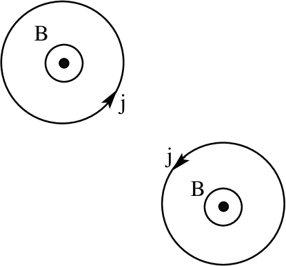
Figure 25: Two vortices and their eddy currents.

Appendix C Map between different forms of the action

An alternate form of the action that we have used early in our simulations is

$$S^{\prime}[\phi]=\frac{1}{t^{\prime}}\int d^{2}x~{}\left\{\frac{1}{2}[{\partial}_{\mu}\phi^{\prime}(x)]^{2}-g^{\prime}\cos(2\phi^{\prime}(x))\right\}$$ (50)

This can be related to the action in the body of the paper, Eq. (1), by defining $\phi(x)=2\phi^{\prime}(x)$ and relating $(t,g)$ to $(t^{\prime},g^{\prime})$ appropriately:

$$t=4t^{\prime},\quad g=4g^{\prime}$$ (51)

In Hasenbusch et al. (1994) the following convention is used:

$$S[\varphi]=\int d^{2}x~{}\left\{\frac{1}{2\beta}({\partial}_{\mu}\varphi)^{2}-z\cos(2\pi\varphi)\right\}$$ (52)

The map is then

$$\varphi=\frac{1}{2\pi}\phi,\quad\beta=\frac{t}{4\pi^{2}},\quad z=\frac{g}{t}$$ (53)

The thicknesses are related by

$${\sigma}_{H}^{2}=\frac{1}{4\pi^{2}}{\sigma}_{J}^{2}$$ (54)

where on the l.h.s. there is the Hasenbusch et al. convention, and on the r.h.s. is ours. As a result we end up with the prediction (29) from their result

$${\sigma}_{H}^{2}\simeq\frac{\beta}{\pi}\ln L+\text{const.}$$ (55)

Appendix D Domain analysis

For every configuration, the values of $\phi$ tend to group together into distinct domains during the thermalization of the system. Plotting the system in terms of x, y, and $\phi$ yields a $L\times L$ scatter plot of particles as seen in Fig. 21. For this particular configuration the potential barrier is low enough, and the temperature is high enough that sites are able to tunnel to several domains above and below $\phi=0$, known as the threshold.

The combination of fugacity and temperature for used to produce the configuration plotted in Fig. 21 makes it easy for an algorithm to recognize the clusters. In particular, it allows K-means, a prototype-based cluster algorithm, to efficiently identify the clusters and their centroids. One major issue that is present in using K-means, however, is that this algorithm requires a predefined cluster count, which is not easily recognizable for large lattice sizes; and due to the nature of the field-versus-site scattering, the commonly-used elbow method is not inherently helpful. We therefore used an alternative: density-based cluster definitions. Here the cluster count is defined using the DBSCAN method, following the format of using the $k-dist$ values to define cluster radius and minimum point threshold. Once $k$ number of cluster radii (called $Eps$) are identified, the algorithm uses K-means to classify those clusters. To aid in speeding up the process, centroids $c_{1}...c_{k}$ are initialized within the local space of each $Eps_{j}$, automatically assigning identified core points and border points to respective cluster $c_{j}$. For any points missed, we simply follow ${\rm argmin}\,D(x_{i},c_{j})$, where $D$ is distance, assigning the noise point $x_{i}$ to closest cluster $c_{j}$.

The algorithm is quick and efficient, but is still not powerful enough when applied to even larger lattice sizes coupled with small deviations of $\phi$. Many configurations of this form can be too complex for this algorithm. A work-around for this is to analyze extremely large amounts of sites is to take the configuration data and project it onto a 2d plane using principle component analysis (PCA). In PCA, a system with a certain amount of unlabeled data is selected to form a $s$-dimensional sample space. The covariance matrix is then computed as

$$\Sigma=\begin{pmatrix}\sigma_{1,1}&\sigma_{1,2}&\cdots&\sigma_{1,j}\\ \sigma_{2,1}&\sigma_{2,2}&\cdots&\sigma_{2,j}\\ \vdots&\vdots&\ddots&\vdots\\ \sigma_{i,1}&\sigma_{i,2}&\cdots&\sigma_{i,j}\end{pmatrix}$$ (56)

Where $\sigma_{i,i}$ is the variance and $\sigma_{i,j}$ is the covariance. The eigenvalues and eigenvectors are calculated from $\Sigma$, giving a set of potential axes (eigenvectors) that the data could be projected upon. The $j$ eigenvectors with the greatest eigenvalues are chosen and combined with the the $s$-dimensional sample space to form a $s\times j$-dimensional matrix $D$, the reduced subspace. The original samples $X$ are then transformed onto the new subspace $Y$

$$Y=D^{T}\times X$$ (57)

In terms of our data, we considered the sample space of the configurations as a fibre bundle instead of just using the singular $\phi$ data generated by the simulation. A fibre bundle is, for our simple theory, the product of the base space and the target space. Considering the analysis in terms of a fibre bundle allows us to observe our PCA sample space with three features (x, y, and $\phi$) instead of just $\phi$. This gives depth to our analysis, allowing for the cluster algorithm to identify the clusters quickly for a large number of increasingly large lattice sizes without any loss in accuracy. Fig. 26 shows the PCA of a configuration with a lattice size of 256. Computation time is cut down by a factor of two and the cluster count and cluster width is not compromised.

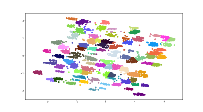
Figure 26: PCA of (thermalized) configuration 1000 for $L=256$, $y=4$, $t=1$.

Appendix E Hard core repulsion

It is straightforward enough to implement the hard-core repulsion in the Coulomb gas model. For instance the fugacity expansion of the partition function as presented in the main text is

$$Z_{\text{CG}}=\sum_{n\in 2{\bf Z}}\frac{y^{n}}{n!}\int d^{2}x_{1}\cdots d^{2}x_{n}\sum_{\{{\epsilon}\}}\prod_{i<j}(\mu|x_{i}-x_{j}|)^{{\epsilon}_{i}{\epsilon}_{j}t/2\pi}$$ (58)

where $y=g/2t$. Hard-core repulsion replaces this with

$$Z_{\text{CG-h.c.r.}}=\sum_{n\in 2{\bf Z}}\frac{y^{n}}{n!}\int d^{2}x_{1}\cdots d^{2}x_{n}\sum_{\{{\epsilon}\}}\prod_{i<j}\theta(|x_{i}-x_{j}|-R)(\mu|x_{i}-x_{j}|)^{{\epsilon}_{i}{\epsilon}_{j}t/2\pi}$$ (59)

so that the integrand vanishes for $|x_{i}-x_{j}|<R$ for any pair $i,j$. Now the question is, how would this change the continuum theory—i.e., what becomes of the sine-Gordon model that this theory is dual to in the absence of the hard-core repulsion? One path to formulating an answer is to represent the Heaviside unit step function as

$$\theta(x)=\int\frac{d\omega}{2\pi}\frac{-ie^{i\omega x}}{\omega-i{\epsilon}}$$ (60)

where as usual ${\epsilon}>0$ is an infinitesmal number that provides a pole prescription. Thus we obtain the expression

$$Z_{\text{CG-h.c.r.}} = \sum_{n\in 2{\bf Z}}\frac{y^{n}}{n!}\int d^{2}x_{1}\cdots d^{2}x_{n}\sum^{\prime}_{\{{\epsilon}\}}\prod_{i<j}\int\frac{d\omega_{ij}}{2\pi}\frac{-ie^{i\omega_{ij}|x_{i}-x_{j}|}}{\omega_{ij}-i{\epsilon}}(\mu|x_{i}-x_{j}|)^{{\epsilon}_{i}{\epsilon}_{j}t/2\pi}$$ (61)

$$= \sum_{n\in 2{\bf Z}}\frac{y^{n}}{n!}\int d^{2}x_{1}\cdots d^{2}x_{n}\sum^{\prime}_{\{{\epsilon}\}}\prod_{i<j}\int\frac{d\omega_{ij}}{2\pi}\frac{-i}{\omega_{ij}-i{\epsilon}}e^{i\omega_{ij}|x_{i}-x_{j}|+({\epsilon}_{i}{\epsilon}_{j}t/2\pi)\ln|x_{i}-x_{j}|}$$

If we define

$$\omega_{ij}=({\epsilon}_{i}{\epsilon}_{j}t/2\pi)\omega^{\prime}_{ij}$$ (62)

then the expression becomes more amenable to intepretation:

$$Z_{\text{CG-h.c.r.}} = \sum_{n\in 2{\bf Z}}\frac{y^{n}}{n!}\int d^{2}x_{1}\cdots d^{2}x_{n}\sum^{\prime}_{\{{\epsilon}\}}\prod_{i<j}\int\frac{d\omega_{ij}}{2\pi}\frac{-i}{\omega_{ij}-i{\epsilon}}e^{({\epsilon}_{i}{\epsilon}_{j}t/2\pi)(i\omega^{\prime}_{ij}|x_{i}-x_{j}|+\ln|x_{i}-x_{j}|}$$ (63)

Thus we posit a differential operator $D(\omega)$ that has Green’s function

$$G(\omega;x,y)=i\omega|x_{i}-x_{j}|+\ln|x_{i}-x_{j}|$$ (64)

Obviously it is some generalization of the 2d Laplacian.

References

- Berezinskii (1971) V. Berezinskii, Soviet Physics JETP 32, 493 (1971).
- Kosterlitz and Thouless (1973) J. M. Kosterlitz and D. J. Thouless, J. Phys. C6, 1181 (1973).
- Benfatto et al. (2013) L. Benfatto, C. Castellani, and T. Giamarchi, in 40 years of Beresinskii-Kosterlitz-Thouless theory, edited by J. V. José (World Scientific, Singapore, 2013) pp. 161–199, 1201.2307 .
- Giedt and Flamino (2018) J. Giedt and J. Flamino, Proceedings, 35th International Symposium on Lattice Field Theory (Lattice 2017): Granada, Spain, June 18-24, 2017, EPJ Web Conf. 175, 14003 (2018), arXiv:1710.03188 [hep-lat] .
- Chui and Weeks (1976) S. Chui and J. Weeks, Phys. Rev. B14, 4978 (1976).
- Chui and Weeks (1978) S. Chui and J. Weeks, Phys. Rev. Lett. 40, 733 (1978).
- Coleman (1975) S. R. Coleman, Phys. Rev. D11, 2088 (1975), [,128(1974)].
- Hasenbusch et al. (1994) M. Hasenbusch, M. Marcu, and K. Pinn, Physica A211, 255 (1994), arXiv:hep-lat/9408005 [hep-lat] .
- Duane et al. (1985) S. Duane, A. Kennedy, B. Pendelton, and D. Roweth, Phys. Lett. 195, 216 (1985).
- Ferreira and Toral (1993) A. Ferreira and R. Toral, Phys. Rev. E47, 3848 (1993).
- Espriu et al. (1997) D. Espriu, V. Koulovassilopoulos, and A. Travesset, Phys. Rev. D56, 6885 (1997), arXiv:hep-lat/9705027 [hep-lat] .
- Catterall and Karamov (2002) S. Catterall and S. Karamov, Phys. Lett. B528, 301 (2002), arXiv:hep-lat/0112025 [hep-lat] .
- Kosterlitz (1974) J. M. Kosterlitz, J. Phys. C7, 1046 (1974).
- Amit et al. (1980) D. J. Amit, Y. Y. Goldschmidt, and G. Grinstein, J. Phys. A13, 585 (1980).
- Zinn-Justin (2002) J. Zinn-Justin, Quantum Field Theory and Critical Phenomena (4th Edition) (Oxford University Press, New York, 2002).
- Samuel (1978) S. Samuel, Physical Review D18, 1916 (1978).
- Mudry (2014) C. Mudry, Lecture notes on field theory in condensed matter physics (World Scientific, New Jersey, 2014).
- Halperin and Nelson (1979a) B. I. Halperin and D. R. Nelson, Journal of Low Temperature Physics 36, 599 (1979a).
- ’t Hooft (1994) G. ’t Hooft, Under the spell of the gauge principle (World Scientific, Singapore, 1994).
- Fradkin (2013) E. Fradkin, Field theory of condensed matter physics, 2nd edition (Cambridge University Press, Cambridge, UK, 2013).
- Halperin and Nelson (1978) B. Halperin and D. Nelson, Phys. Rev. Lett. 41, 121 (1978).
- Halperin and Nelson (1979b) B. Halperin and D. Nelson, Phys. Rev. B19, 2457 (1979b).
- Young (1979) A. Young, Phys. Rev. B19, 1855 (1979).
- Nelson (1978) D. Nelson, Phys. Rev. B18, 2318 (1978).
- Pordes and et al. (2007) R. Pordes and et al., J. Phys. Conf. Ser. 78, 012057 (2007).
- Sfiligoi et al. (2009) I. Sfiligoi, D. C. Bradley, B. Holzman, P. Mhashilkar, S. Padhi, and F. Wurthwein, 2009 WRI World Congress on Computer Science and Information Engineering 2, 428 (2009).
- Towns et al. (2014) J. Towns, T. Cockerill, M. Dahan, I. Foster, K. Gaither, A. Grimshaw, V. Hazlewood, S. Lathrop, D. Lifka, G. D. Peterson, R. Roskies, J. R. Scott, and N. Wilkins-Diehr, Computing in Science & Engineering 16, 62 (2014).
- Gradshteyn and Ryzhik (1994) I. S. Gradshteyn and I. M. Ryzhik, Table of Integrals, Series & Products, Fifth Edition, edited by A. Jeffrey (Academic Press, San Diego, California, 1994).