Low-Rank Semidefinite Programs via Bilinear Factorization

A biconvex optimization for solving semidefinite programs via bilinear factorization

Abstract

Many problems in machine learning can be reduced to learning a low-rank positive semidefinite matrix (denoted as $Z$), which encounters semidefinite program (SDP). Existing SDP solvers by classical convex optimization are expensive to solve large-scale problems. Employing the low rank of solution, Burer-Monteiro’s method reformulated SDP as a nonconvex problem via the quadratic factorization ($Z$ as $XX^{\top}$). However, this would lose the structure of problem in optimization. In this paper, we propose to convert SDP into a biconvex problem via the bilinear factorization ($Z$ as $XY^{\top}$), and while adding the term $\frac{\gamma}{2}\left\|X-Y\right\|_{F}^{2}$ to penalize the difference of $X$ and $Y$. Thus, the biconvex structure (w.r.t. $X$ and $Y$) can be exploited naturally in optimization. As a theoretical result, we provide a bound to the penalty parameter $\gamma$ under the assumption of $L$-Lipschitz smoothness and $\sigma$-strongly biconvexity, such that, at stationary points, the proposed bilinear factorization is equivalent to Burer-Monteiro’s factorization when the bound is arrived, that is $\gamma>\frac{1}{4}(L-\sigma)_{+}$. Our proposal opens up a new way to surrogate SDP by biconvex program. Experiments on two SDP-related applications demonstrate that the proposed method is effective as the state-of-the-art.

1 Introduction

In this paper, we consider the minimization of a smooth convex function over the cone of symmetric positive semidefinite (PSD) matrices, that is

$$\min_{Z\in{\mathbb{S}}_{+}^{n}}\dot{f}(Z),$$ (1)

where ${\mathbb{S}}_{+}^{n}=\{Z|Z=Z^{\top},Z\succeq 0,Z\in{\mathbb{R}}^{n\times n}\}$. Many problems in machine learning can be reformulated as (1). Prominent examples include adaptive clustering (Royer, 2017), sparse PCA (D’aspremont et al., 2007), connected subgraph detection (Aksoylar et al., 2017), nonlinear dimensionality reduction (Weinberger et al., 2004), kernel learning (Zhuang et al., 2011), distance metric learning (Xing et al., 2002), multitask learning (Obozinski et al., 2009), streaming model (Tropp et al., 2017), matrix completion (Srebro et al., 2005), and inference in graphical model (Erdogdu et al., 2017), etc..

Although general interior-point methods can be applied to solve the convex problem (1) with linear convergence, they suffer from exceedingly high computational cost per-iteration, which restrict their capabilities to solving SDP. Another solution is to employ the projected gradient (PG) method (Nesterov and Nemirovski, 1994) or Frank-Wolfe (FW) method (Frank and Wolfe, 1956), where the PG method needs to compute the projection into PSD domain at each iteration, and FW needs to solve a linear optimization problem under PSD constraint. However, projection into ${\mathbb{S}}_{+}^{n}$ are time-consuming, and a linear optimization over PSD constraint barely is illposed because ${\mathbb{S}}_{+}^{n}$ is unbounded.

Generally speaking, PSD constraint is the most challenging aspect of solving (1). In order to overcome this difficulty, Burer-Monteiro’s method (Burer and Monteiro, 2003; Journeé et al., 2010; Li and Tang, 2017; Srinadh et al., 2016; Zheng and Lafferty, 2015) proposed to factorize $Z$ quadraticly as $XX^{\top}$, and surrogate (1) by a nonconvex program as

$$\min_{X\in{\mathbb{R}}^{n\times r}}\ddot{f}(X)=\dot{f}(XX^{\top}),$$ (2)

where $X$ is a real matrix and $r\ll n$ if $Z$ is low-rank. Compared with (1), problem (2) does not have PSD constraint, but the objective becomes a nonconvex function. To solve problem (2), we refer to the existing results in (Burer and Monteiro, 2003; Journeé et al., 2010; Li and Tang, 2017; Srinadh et al., 2016; Zheng and Lafferty, 2015), and then from the perspectives therein we can summarize the connections between (1) and (2) as follows:

1. If ${\bar{X}}$ is rank deficient, a stationary point ${\bar{X}}$ of problem (2) (i.e. $\nabla\ddot{f}({\bar{X}})=0$) either corresponds to the global optimum ${\bar{Z}}={\bar{X}}{\bar{X}}^{T}$ for problem (1) or is a strict saddle point (which includes a local maximum) of $\ddot{f}$.

2. If ${\bar{X}}$ is rank deficient, any local minimizer ${\bar{X}}$ of problem (2) corresponds to the optimum ${\bar{Z}}={\bar{X}}{\bar{X}}^{T}$ for problem (1).

The above results show that a local minimizer ${\bar{X}}$ of (2) will solve (1) if beforehand set $r>rank({\bar{X}})$ (i.e., ${\bar{X}}$ is rank deficient, refer to (Li and Tang, 2017) for more details). The recent work (Ge et al., 2017) further claimed that: for (2), no high-order saddle points exist, and all local minimizers are also globally optimal. Nevertheless, the factorized formulation (2) would bring higher-order nonlinearity, and thus lose the structure of problem in subsequent optimization.

Different from Burer-Monteiro’s method by factorizing $Z$ quadraticly as $XX^{\top}$ as in (2), in this paper we propose a novel surrogate that factorizing $Z$ bilinearly as $XY^{\top}$, and penalizing the difference between $X$ and $Y$ (here is $\frac{\gamma}{2}\left\|X-Y\right\|_{F}^{2}$). Specifically, let $Z=XY^{\top}$, we convert SDP (1) into a biconvex problem with the addition of a Courant penalty (Nocedal and Wright, 2006), in which the resultant subproblems are convex w.r.t. $X$ and $Y$ respectively. We will show that the proposed surrogate contributes to faster computation to optimize (1) especially when $\dot{f}(\cdot)$ is a quadratic function.

1.1 Related Work

The interior point method (Nesterov and Nemirovski, 1994) can produce highly accurate solutions for SDP problem. However, it is not scalable because at least $O(n^{3})$ time and $O(n^{2})$ space are needed in each iteration. Moreover, the interior point method is difficult to utilize additional information about the problem structure, such as that the target matrix is low-rank. To exploit low-rank structure, a popular approach for solving SDP is the Frank-Wolfe (FW) algorithm (Jaggi, 2013), which is based on sparse greedy approximation. For smooth problems, the complexity of FW is $O(N/\epsilon^{1.5})$ arithmetic operations (Jaggi, 2013), that is: $O(1/\epsilon)$ iterations are demanded to converge to an $\epsilon$-accurate solution, and in each iteration, $O(N\log(n)/\sqrt{\epsilon})$ arithmetic operations are needed, where $N$ is the number of nonzero entries in gradient. When the gradient of objective is dense, FW can still be expensive.

Alternatively, as $Z$ in (1) is symmetric and positive semidefinite, it can be factorized quadraticly as $XX^{\top}$. Thus, problem (1) can then be reformulated as a nonconvex program as (2) (Burer and Monteiro, 2003). It is known that a local minimizer ${\bar{X}}$ of (2) corresponds to a minimizer of (1) if ${\bar{X}}$ is rank-deficient (Burer and Monteiro, 2003; Journeé et al., 2010; Li and Tang, 2017). For linear objective and linear constraints, the nonconvex program (2) has been solved with L-BFGS (Burer and Monteiro, 2003; Nocedal and Wright, 2006). However, the convergence properties are unclear when solving a general nonconvex program by L-BFGS. Block-cyclic coordinate minimization has been used in (Hu et al., 2011) to solve a special nonconvex program of SDP, but a closed-form solution is preferred in each block coordinate update.

1.2 Notation

We set $(\cdot)_{+}=\max\{\cdot,0\}$. The transpose of vector or matrix is denoted by the superscript ^⊤. The identity matrix is denoted by $I$ with appropriate size. For a matrix $A=[a_{ij}]$, $\text{tr}(A)$ is its trace, $\left\|A\right\|_{F}=(\sum_{ij}a_{ij}^{2})^{1/2}$ is its Frobenius norm, $\left\|\cdot\right\|_{2}$ is its spectral norm (i.e., maximal singular value), and ${\rm{vec}}(A)$ unrolls $A$ into a column vector. For two matrices $A,B$, $\langle A,B\rangle=\text{tr}(A^{\top}B)$, and $A\otimes B$ is their Kronecker product. If $g(u,v)$ is a function w.r.t. both first-variable $u$ and second-varible $v$, then $g(u,\cdot)$ is a function of only first-variable with a (or any) constant for the second-variable, while $g(\cdot,v)$ is a function of only second-variable with a (or any) constant for the first-variable, and naturally $\nabla_{1}g(\cdot,\cdot)$ and $\nabla_{2}g(\cdot,\cdot)$ are the partial derivatives of first-variable function and second-variable function respectively. To simplify the notation of derivative, to the functions in (1)(2)(3)(4), we agree as follows

$$\nabla\dot{f}(Z)=\nabla_{Z}\dot{f}(Z)$$

$$\nabla\ddot{f}(X)=\nabla_{X}\ddot{f}(X)$$

$$\nabla_{1}F(X,\cdot)=\nabla_{X}F(X,\cdot),\ \nabla_{2}F(\cdot,Y)=\nabla_{Y}F(\cdot,Y)$$

$$\nabla_{1}f(X,\cdot)=\nabla_{X}f(X,\cdot),\ \nabla_{2}f(\cdot,Y)=\nabla_{Y}f(\cdot,Y).$$

2 Problem Formulation

2.1 Motivation

For current large-scale optimization in machine learning, the first-order optimization methods, such as (accelerated/stochastic) gradient descent, are popular because of their computational simplicity. In the class of these methods, the most expensive operation usually lies in repeatedly searching a stepsize for objective descent at each iteration, which involves computation of the objective many times. If a good stepsize is possible in an analytical and simple form, the computation complexity would be decreased greatly.

However, a simple stepsize is impossible in (2) even if $\dot{f}$ is a simple quadratic function. This is because that when $\dot{f}$ in (1) is quadratic w.r.t. $Z$, the objective $\ddot{f}$ in (2) rises into a quartic function w.r.t. $X$, such that the stepsize search in (2) involves some complex computations including constructing the coefficients of a quartic polynomial, solving a cubic equation and selecting the resulted different solutions (Burer and Choi, 2006). Again, this needs compute the objective many times.

The above difficulties motivate us to propose biconvex formulation (3) instead of (2). In each subproblem of (3), the stepsize search is usually easier than in (2). For example, when $\dot{f}$ is a quadratic function, the subobjective $F(X,Y;\gamma)$ or $F(X,Y;\gamma)$ of (3) is still quadratic w.r.t. $X$ or $Y$ respectively. Hence, the optimal stepsize to descend objective w.r.t $X$ or $Y$ is analytical, simple and unique for (3) ((22) is an example).

2.2 Problem Formulation

Instead of factorizing $Z$ quadraticly as $XX^{\top}$, we factorize $Z$ bilinearly as $XY^{\top}$, and penalize the difference between $X$ and $Y$, which can be formulated as

$$\min_{X,Y\in{\mathbb{R}}^{n\times r}}F(X,Y;\gamma)\equiv f(X,Y)+{\gamma\over 2}\left\|X-Y\right\|_{F}^{2},$$ (3)

where $\gamma>0$ is a penalty parameter and $f(X,Y)$ is defined as

$$f(X,Y)=\dot{f}(XY^{\top})\ (\text{or}\ f(X,Y)=\dot{f}(YX^{\top})).$$ (4)

Note that the penalty term in (3) is the classic quadratic (or Courant) penalty for the constraint $X=Y$. In general, problem (3) approaches problem (2) only when $\gamma$ goes to infinity. However, we will show (in Theorem 1) that $\gamma$ can be bounded (i.e., does NOT require $\gamma\rightarrow+\infty$) if $\ddot{f}$ (or $\dot{f}$) is Lipschitz smooth, such that when $\gamma$ is larger than that bound, (3) is equivalent to (2) in that a stationary point $({\bar{X}},{\bar{Y}})$ of (3) provides ${\bar{X}}$ as a stationary point of (2). Hence, any local minimizer of (3) will produce optimal solution of (1) if $r$ is set as large as enough. Moreover, it will be shown that the objective in (3) is biconvex, and thus we can choose a convex optimization algorithm to decrease the objective function $F$ w.r.t. $X$ and $Y$ alternately. Consequently, this opens a door to surrogate SDP by biconvex program.

2.3 Contributions

Our main contributions can be summarized as follows:

1. We propose a biconvex formulation (3) to the surrogate the SDP problem (1). This opens up a new path to solve many SDP-related problems using biconvex optimization.

2. We propose a theoretical bound to the penalty parameter $\gamma$, thus does NOT require $\gamma\rightarrow+\infty$. This bridges the stationary point of (3) to the stationary point of (2) if $\gamma$ is set as larger than this bound.

3. We show that problem (3) is evidently easier to be solved than (2) if $\dot{f}(\cdot)$ is especially a quadratic function (according to our motivation). This has been validated on two SDP-related applications in the experimental section.

3 Proposed Algorithm

3.1 Biconvex Penalty

We first give the definition of biconvexity as follows

Definition 1.

$g(\cdot,\cdot)$ is biconvex if for any $x_{i},y_{i}$, and any $0\leq{\alpha}_{i},\beta_{i}\leq 1$ ($i=1,2$) such that ${\alpha}_{1}+{\alpha}_{2}=\beta_{1}+\beta_{2}=1$, we have $g({\alpha}_{1}x_{1}+{\alpha}_{1}x_{2},\beta_{1}y_{1}+\beta_{2}y_{2})\leq{\alpha}_{1}\beta_{1}g(x_{1},y_{1})+{\alpha}_{1}\beta_{2}g(x_{1},y_{2})+{\alpha}_{2}\beta_{1}g(x_{2},y_{1})+{\alpha}_{2}\beta_{2}g(x_{2},y_{2})$. Namely, $g(\cdot,y)$ and $g(x,\cdot)$ are convex respectively with fixed $x$ and $y$.

Definition 2.

$g(\cdot)$ is $\hat{L}$-Lipschitz smooth if for any $x_{1},x_{2}$, we have $\|\nabla g(x_{2})-\nabla g(x_{1})\|\leq\hat{L}\|x_{2}-x_{1}\|$ with $0\leq\hat{L}<+\infty$.

The following Proposition shows that $f$ in (4) and $F$ in (3) are biconvex if $\dot{f}$ in (1) is convex.

Proposition 1.

If $\dot{f}$ in (1) is convex w.r.t. $Z$, then $f$ in (4) and $F$ in (3) are biconvex w.r.t. $X$ and $Y$.

Below we assume that $\dot{f}$, $\ddot{f}$ and $f$ satisfy the following assumptions.

Assumption 1.

$\dot{f}$ (and thus $f$) is coercive, namely satisfying $\lim\limits_{\|Z\|\rightarrow+\infty}\frac{\dot{f}(Z)}{\|Z\|}\rightarrow+\infty$ for $\forall Z\in{\mathbb{R}}^{n\times n}$. This implies that the sublevel set $\mathcal{L}_{c}=\{(X,Y)|f(X,Y)\leq c\}$ is bounded.

Assumption 2.

For $\forall X,Y,X_{1},X_{2},Y_{1},Y_{2}\in{\mathbb{R}}^{n\times r}$,

1. $\ddot{f}(\cdot)$ is $L$-Lipschitz smooth, that is

   $$\ddot{f}(Y)-\ddot{f}(X)-\text{tr}[(Y-X)^{\top}\nabla\ddot{f}(X)]\leq\frac{L}{2}\left\|Y-X\right\|_{F}^{2},$$ (5)

   It is easy to know that (5) implies

   $$\text{tr}[(\nabla\ddot{f}(Y)-\nabla\ddot{f}(X)){{}^{\top}}(Y-X)]\leq L\left\|Y-X\right\|_{F}^{2}.$$ (6)

2. $f(X,\cdot)$ and $f(\cdot,Y)$ are $\sigma$-strongly biconvex, that is

   $$f(X_{2},\cdot)-f(X_{1},\cdot)-\text{tr}[(X_{2}-X_{1})^{\top}\nabla_{1}f(X_{1},\cdot)]\geq\frac{\sigma}{2}\left\|X_{2}-X_{1}\right\|_{F}^{2},$$ (7)

   $$f(\cdot,Y_{2})-f(\cdot,Y_{1})-\text{tr}[(Y_{2}-Y_{1})^{\top}\nabla_{2}f(\cdot,Y_{1})]\geq\frac{\sigma}{2}\left\|Y_{2}-Y_{1}\right\|_{F}^{2}.$$ (8)

Remark 1.

It is obvious that for $\forall Y\in{\mathbb{R}}^{n\times r}$

$$\nabla\ddot{f}(Y)=2\nabla_{1}f(Y,Y)=2\nabla_{2}f(Y,Y)=2\nabla\dot{f}(YY{{}^{\top}})Y.$$ (9)

From (9), the condition of Lipschitz smooth for $\ddot{f}(\cdot)$ is quivalent to the condition of Lipschitz smooth for $\dot{f}(\cdot)$ under Assumption 1. Hence, in (Srinadh et al., 2016), $L$ is estimated as $16(M\left\|X_{0}\right\|_{2}+\left\|\nabla\dot{f}(Z_{0})\right\|_{2})$ wehre $M$ is a uniform upper bound on the largest eigenvalue of the Hessian $\nabla^{2}\dot{f}(Z_{0})$, $Z_{0}=X_{0}X_{0}{{}^{\top}}$ and $X_{0}$ is a starting point in ierative optimization.

3.2 The Theoretical Bound

In the following Theorem, we provide a theoretical bound to penalty parameter $\gamma$ to bridge problems (3) and (2), and thus problem (1).

Theorem 1.

Assume that $({\bar{X}},{\bar{Y}})$ is a stationary point of problem (3), then ${\bar{X}}={\bar{Y}}$ if $\gamma>\frac{1}{4}(L-\sigma)_{+}$.

Corollary 1.

Assume that the condition of Theorem 1 is satisfied, then we have: (i) ${\bar{X}}$ is a stationary point of (2) if $({\bar{X}},{\bar{Y}})$ is a stationary point of (3); (ii) ${\bar{X}}$ is a local minimizer of (2) if $({\bar{X}},{\bar{Y}})$ is a local minimizer of (3).

Remark 2.

Following Corollary 1, a local minimizer $({\bar{X}},{\bar{Y}})$ of (3) provides ${\bar{X}}$ as a local minimizer of (2) if $\gamma>\frac{1}{4}(L-\sigma)_{+}$. Furthermore, the produced ${\bar{Z}}(={\bar{X}}{\bar{X}}^{\top})$ will solve (1) if the condition of rank deficiency (i.e., $r>rank({\bar{X}})$) is satisfied (Li and Tang, 2017).

3.3 Our Algorithm

Now we focus on solving (3) under the assumption that the penalty parameter $\gamma$ satisfies Theorem 1. Depending on the convexity of subproblems, we can solve (3) in alternate convex search. Specifically, we can solve the convex subproblem w.r.t. $X$ with fixed $Y$ and the convex subproblem w.r.t. $Y$ with fixed $X$ alternately, that is

$$X_{k} = \operatorname{arg\,min}\limits_{X\in{\mathbb{R}}^{n\times r}}F(X,Y_{k-1};\gamma);$$ (10)

$$Y_{k} = \operatorname{arg\,min}\nolimits_{Y\in{\mathbb{R}}^{n\times r}}F(X_{k},Y;\gamma).$$ (11)

In fact, it makes sense to solve (10) and (11) only inexactly. An example is multiconvex optimization (Xu and Yin, 2013), in which an alternating proximal gradient descent was proposed to solve multiconvex objective.

We first give a brief introduction to accelerated proximal gradient (APG) descent method, and then fuse it into our algorithm. A well-known APG method is FISTA (Beck and Teboulle, 2009), which was proposed to solve convex composite objective as like as

$$\min\nolimits_{x}\ell(x)+h(x),$$

where $\ell(x)$ is differentiable loss and $h(x)$ is nondifferentiable regularizer. When $h(x)=0$ (i.e., ’proximal’ is absent, as used in our case later), FISTA is degenerated into computing the sequence $\{x_{s}\}$ via the iteration

$$\left\{\begin{aligned} &t_{s}=\frac{1}{2}\left(1+\sqrt{1+4s^{2}_{s-1}}\right),\omega_{s}=\frac{t_{s-1}-1}{t_{s}},\\ &\hat{x}_{s-1}=x_{s-1}+\omega_{s}(x_{s-1}-x_{s-2}),\\ &x_{s}=\hat{x}_{s-1}-\tau_{s}\nabla_{x}\ell(\hat{x}_{s-1}).\end{aligned}\right.$$ (12)

where $\tau_{s}$ is stepsize for descent.

We can apply (12) (as a degenerated FISTA) to (10) and (11). Since $F(X,Y_{k-1};\gamma)$ is convex and differentiable, regarding it as $\ell(\cdot)$ we can inexactly solve (10) by using (12) as the process of inner iterations. Analogously, we can inexactly solve (11) by using (12) as inner procedure. The smaller the number of inner iterations, the faster the interaction between the updates of $X_{k}$ and $Y_{k}$ each other. Specially, if we set $1$ as the number of inner iterations to inexactly solve (10) and (11) respectively, the optimization for them can be realized as Algorithm 1 (except steps $4$, $7$ and $11$), that is our alternating accelerated gradient descent (AAGD) algorithm, where steps $5$ and $6$ inexactly solve (10) and steps $8$ and $9$ inexactly solve (11).

Algorithm 1 Alternating Accelerated Gradient Descent (AAGD).

1:  Initialization: $X_{0}$, $Y_{0}$, $X_{-1}=X_{0}$, $Y_{-1}=Y_{0}$, $t_{0}=1$.

2:  for $k=1,\ldots,$ do

3:     $t_{k}=\frac{1}{2}\left(1+\sqrt{1+4t^{2}_{k-1}}\right),\omega_{k}=\frac{t_{k-1}-1}{t_{k}}$,

4:     estimate the penalty parameter $\gamma_{\frac{k}{2}}$;

5:     $\hat{X}_{k-1}=X_{k-1}+\omega_{k}(X_{k-1}-X_{k-2})$;

6:     $X_{k}=\hat{X}_{k-1}-\tau_{k}^{X}\nabla_{1}F(\hat{X}_{k-1},Y_{k-1};\gamma_{\frac{k}{2}})$;

7:     estimate the penalty parameter $\gamma_{k}$;

8:     $\hat{Y}_{k-1}=Y_{k-1}+\omega_{k}(Y_{k-1}-Y_{k-2})$;

9:     $Y_{k}=\hat{Y}_{k-1}-\tau_{k}^{Y}\nabla_{2}F(X_{k},\hat{Y}_{k-1};\gamma_{k})$;

10:     if a stopping criterion is satisfied then

11:        return ${\bar{Z}}=Y_{k}Y^{\top}_{k}$  (or  $X_{k}X^{\top}_{k}$).

12:     end if

13:  end for

From another perspective, Algorithm 1 (except steps $4$ and $7$ and $11$) can be regarded as a degenerated realization (with a slight difference in rectified $\omega_{k}$) of alternating proximal gradient method in multiconvex optimization (Xu and Yin, 2013). Hence, the convergence of Algorithm 1 is solid following (Xu and Yin, 2013).

4 Applications

4.1 NPKL: nonparametric kernel learning

Given $n$ patterns, let ${\mathcal{M}}$ be the must-link set containing pairs that should belong to the same class, and ${\mathcal{C}}$ be the cannot-link set containing pairs that should not belong to the same class. We use one of formulations in (Zhuang et al., 2011), which learns a kernel matrix using the following SDP problem

$$\mathop{\min}\limits_{Z\in{\mathbb{S}}_{+}^{n}}\;\dot{f}^{(1)}(Z)=\frac{1}{2}\sum_{\{j,i\}\in{\mathcal{T}}}(Z_{ji}-T_{ji})^{2}+\lambda\text{tr}(Z\Delta)$$ (13)

where $Z=[Z_{ji}]\in{\mathbb{R}}^{n\times n}$ is the target kernel matrix, $\Delta$ is the graph Laplacian matrix of the data, ${\mathcal{T}}={\mathcal{M}}\cup{\mathcal{C}}\cup\{j=i\}$, $T=[T_{ji}]$ with $T_{ji}=1$ if $\{j,i\}\in{\mathcal{M}}$ or $j=i$, and 0 if $\{j,i\}\in{\mathcal{C}}$, and $\lambda$ is a tradeoff parameter. The first term of objective in (13) measures the difference between $Z_{ji}$ and $T_{ji}$, and the second term $\text{tr}(Z\Delta)$ encourages smoothness on the data manifold by aligning $Z$ with $\Delta$.

4.1.1 Biconvex reformulation

Let $f^{(1)}(X,Y)=\dot{f}^{(1)}(XY^{\top})$, we have

$$f^{(1)}(X,Y)=\frac{1}{2}\sum_{\{j,i\}\in{\mathcal{T}}}[(\text{tr}(X^{\top}S_{ji}Y))^{2}-2T_{ji}\text{tr}(X^{\top}S_{ji}Y)]$$ (14)

$$+\lambda\text{tr}(X^{\top}\Delta Y)+C$$

$$=\frac{1}{2}{\rm{vec}}(X)^{\top}\hat{{\mathcal{A}}}(Y){\rm{vec}}(X)-{\rm{vec}}(X)^{\top}\hat{{\textit{b}}}(Y)+C$$

where

$$\hat{{\mathcal{A}}}(Y) = (Y^{\top}\otimes I)PP^{\top}(Y^{\top}\otimes I)^{\top},$$

$$\hat{{\textit{b}}}(Y) = (Y^{\top}\otimes I)q,$$

$$P = \sum\limits_{\{j,i\}\in{\mathcal{T}}}{\rm{vec}}(S_{ji}){\rm{vec}}(S_{ji})^{\top},$$

$$q = \sum\limits_{\{j,i\}\in{\mathcal{T}}}T_{ji}{\rm{vec}}(S_{ji})-\lambda{\rm{vec}}(\Delta),$$

$$S_{ji} = I(:,j)(I(i,:))^{\top},$$

and $I$ is denoted as the identity matrix with appropriate size, $I(:,i)$ is the $i$-th column of $I$, $C$ is a constant. Plugging $f=f^{(1)}$ into (3), we have

$$F(X,Y;\gamma)=f^{(1)}(X,Y)+{\gamma\over 2}\left\|X-Y\right\|_{F}^{2}$$

$$= \frac{1}{2}{\rm{vec}}(X)^{\top}{\mathcal{A}}(Y,\gamma){\rm{vec}}(X)-{\rm{vec}}(X)^{\top}{\textit{b}}(Y,\gamma)$$

$$-{\gamma\over 2}{\rm{vec}}(Y)^{\top}{\rm{vec}}(Y)+C$$

where

$${\mathcal{A}}(Y,\gamma) = \gamma I+\hat{{\mathcal{A}}}(Y),$$

$${\textit{b}}(Y,\gamma) = (Y^{\top}\otimes I)(q-\gamma{\rm{vec}}(I)).$$

So, the subproblem about $X$ (corresponding to (10)) is

$$\min\limits_{X\in{\mathbb{R}}^{n\times r}} F(X,Y_{k-1};\gamma_{\frac{k}{2}})$$

$$\Leftrightarrow\min\limits_{X\in{\mathbb{R}}^{n\times r}} \frac{1}{2}{\rm{vec}}(X)^{\top}{\mathcal{A}}^{Y}_{k}{\rm{vec}}(X)-{\rm{vec}}(X)^{\top}{\textit{b}}^{Y}_{k}$$ (15)

where ${\mathcal{A}}^{Y}_{k}={\mathcal{A}}(Y_{k-1},\gamma_{\frac{\gamma}{2}})$, ${\textit{b}}^{Y}_{k}={\textit{b}}(Y_{k-1},\gamma_{\frac{\gamma}{2}})$.

Since $F$ is symmetric in terms of $X$ and $Y$, similar to (15) the subproblem about $Y$ (corresponding to (11)) is

$$\min\limits_{Y\in{\mathbb{R}}^{n\times r}} F(X_{k},Y;\gamma_{k})$$

$$\Leftrightarrow\min\limits_{Y\in{\mathbb{R}}^{n\times r}} \frac{1}{2}{\rm{vec}}(Y)^{\top}{\mathcal{A}}^{X}_{k}{\rm{vec}}(Y)-{\rm{vec}}(Y)^{\top}{\textit{b}}^{X}_{k}$$ (16)

where ${\mathcal{A}}^{X}_{k}={\mathcal{A}}(X_{k},\gamma_{k})$, ${\textit{b}}^{X}_{k}={\textit{b}}(X_{k},\gamma_{k})$.

4.1.2 Estimating the bound of $\gamma$

In practice, $L$ (Lipschitz smooth constant) in Assumption 2 can be estimated dynamically, such that at $k$-th iteration, $L$ can be estimated as similar to (Srinadh et al., 2016) as

$$L\leftarrow L^{k}\approx 16(3\left\|X_{k-1}\right\|_{2}+\left\|\nabla\dot{f}(X_{k-1}X_{k-1}{{}^{\top}})\right\|_{2})$$ (17)

where $\left\|\cdot\right\|_{2}$ is the spectral norm.

From (14), the Hessian of $f^{(1)}(X,Y)$ in terms of variable $X$ is

$$H(Y)=\hat{{\mathcal{A}}}(Y)=(Y^{\top}\otimes I)PP^{\top}(Y^{\top}\otimes I)^{\top}.$$

so $\sigma_{1}$ (strongly convex constant) in Assumption 2 can be estimated as the minimal singular value of $H(Y)$, that is

$$\sigma_{1}=\hat{\sigma}_{\min}(H(Y))\geq\hat{\sigma}_{\min}(PP{{}^{\top}})\hat{\sigma}_{\min}(YY{{}^{\top}})$$ (18)

In practice, $\sigma_{1}$ can be estimated dynamically, such that at $k$-th iteration, which can be approximated as

$$\sigma_{1}\leftarrow\sigma_{1}^{k}\approx\hat{\sigma}_{\min}(PP{{}^{\top}})\hat{\sigma}_{\min}(Y_{k-1}Y_{k-1}{{}^{\top}}).$$ (19)

From the symmetry between $X$ and $Y$, similar to the above, $\sigma_{2}$ can be approximated as

$$\sigma_{2}\leftarrow\sigma_{2}^{k}\approx\hat{\sigma}_{\min}(PP{{}^{\top}})\hat{\sigma}_{\min}(X_{k}X_{k}{{}^{\top}}).$$ (20)

By algorithm 1, the objective $c_{k}=F(X_{k},Y_{k};\gamma)$ is descent as iterations, and Assumption 1 means that the sublevel set $\mathcal{L}_{c_{k}}=\{(X,Y)|f(X,Y)\leq c_{k}\}$ is nonexpensive as iterations. Thus, $L^{k}$ in (17), $\sigma_{1}^{k}$ and $\sigma_{2}^{k}$ in (19)$\sim$(20) are bounded. Meanwhile, we can dynamically set the penalty parameter by Theorem 1 as

$$\gamma_{k}>\frac{1}{4}(L^{k}-\sigma^{k})$$ (21)

where $\sigma^{k}=\min\{\sigma_{1}^{k},\sigma_{2}^{k}\}$. Additionally, we could obtain $L^{k}$ by line search or backtracking.

4.1.3 Computing the optimal stepsizes

The objective functions of (15) and (16) are quadratic, so the optimal stepsize to descend subobjective w.r.t $X$ or $Y$ is analytical, simple and unique, which are provided by the following Proposition.

Proposition 2.

For subproblems (15) and (16), the optimal stepsizes in Algorithm 1 have closed forms as

$$\tau_{k}^{X}=\frac{\left\|d_{k}^{X}\right\|_{F}^{2}}{{d_{k}^{X}}^{\top}{\mathcal{A}}^{Y}_{k}d_{k}^{X}},\ \ \tau_{k}^{Y}=\frac{\left\|d_{k}^{Y}\right\|_{F}^{2}}{{d_{k}^{Y}}^{\top}{\mathcal{A}}^{X}_{k}d_{k}^{Y}}$$ (22)

where $d_{k}^{X}={\rm{vec}}(\nabla_{1}F(\hat{X}_{k-1},Y_{k-1};\gamma_{\frac{k}{2}}))$ and $d_{k}^{Y}={\rm{vec}}(\nabla_{2}F(X_{k},\hat{Y}_{k-1};\gamma_{k}))$.

4.2 CMVU:colored maximum variance unfolding

The colored maximum variance unfolding (CMVU) is a “colored” variants of maximum variance unfolding (Weinberger et al., 2004), subjected to class labels information. The slack CMVU (Song et al., 2008) was proposed as a SDP as

$$\mathop{\min}\limits_{Z\in{\mathbb{S}}_{+}^{n}}\;\dot{f}^{(2)}(Z)=\frac{1}{2}\sum_{\{i,j\}\in{\mathcal{N}}}(Z_{ii}+Z_{jj}-2Z_{ij}-d_{ij})^{2}-\lambda\text{tr}(HZHK).$$ (23)

where $d_{ij}$ denotes the square Euclidean distance between the $i$-th and $j$-th objects, ${\mathcal{N}}$ denotes the set of neighbor pairs, whose distances are to be preserved in the unfolding space, $K$ is a kernel matrix of the labels, $H=[H_{ij}]=[\delta_{ij}-\frac{1}{n}]$ centers the data and the labels in the unfolding space, and $\lambda$ controls the tradeoff between dependence maximization and distance preservation. Let $E_{ij}=I(:,i)-I(:,j)$, (23) can be reformulated as

$$\mathop{\min}\limits_{Z\in{\mathbb{S}}_{n}^{+}}\;\dot{f}^{(2)}(Z)=\frac{1}{2}\sum_{\{i,j\}\in{\mathcal{N}}}(E_{ij}^{\top}ZE_{ij}-d_{ij})^{2}-\lambda\text{tr}(ZHKH).$$

Let $f^{(2)}(X,Y)=\dot{f}^{(2)}(XY{{}^{\top}})$, and viewing $E_{ij}E_{ij}^{\top}$, $-HKH$, $d_{ij}$ as $S_{ji}$, $\Delta$, $T_{ji}$ respectively as in (13), the subproblems about $f^{(2)}$ w.r.t. $X$ and $Y$ can be derived and they are similar to (15) and (16) respectively.

4.3 Complexity Analysis

The per-iteration of Algorithms 1 is inexpensive. It mainly costs ${\mathcal{O}}(nr)$ operations for estimating penalty parameter in $\eqref{eq:ppar}$ since $P$ is a constant needed to be computed only once, and the spectral norm $\left\|X_{k}\right\|_{2}$ or $\left\|\nabla\dot{f}(X_{k-1}X_{k-1}{{}^{\top}})\right\|_{2}$ costs ${\mathcal{O}}(nr)$ usually. As in Proposition 2, it is still ${\mathcal{O}}(nr^{2})$ operations for calculating the optimal stepsizes. The space complexity is scalable because only $O(nr)$ space is needed indeed.

5 Experiments

In this part, we perform experiments on two SDP-related applications in the previous section: NPKL, CMVU and SD.

The proposed algorithm, AAGD in Algorithm 1, will be compared with the following state-of-the-art baselines in solving SDP in (1).

1. FW: accelerated Frank-Wolf algorithm (Laue, 2012) to solve (1);

2. AGD: transform (1) to (2), and solve (2) using the accelerated gradient descent (Ghadimi and Lan, 2016; Li and Lin, 2015). The stepsize search is followed as in (Burer and Choi, 2006).

3. L-BFGS: transform (1) to (2), and solve (2) using limited memory Broyden-Fletcher-Goldfarb-Shanno method (as similar as done in (Burer and Monteiro, 2003)).

4. SQLP: semidefinite-quadratic-linear program (Wu et al., 2009), an interior point method, is specified to quadratic SDP. Naturally, SQLP would be faster than a general purpose SDP-solver to solve a quadratic SDP problem like (13) or (23).

All these algorithms are implemented in Matlab. The stopping condition of FW is reached when the relative change in objective value is smaller than $10^{-6}$, and then the stopping conditions of the others are reached when their objective values are not larger than the final objective value of FW or the number of iterations exceeds $2000$. All experiments are run on a PC with a 3.07GHz CPU and 24GB RAM.

The $r$ (rank of the solution) is automatically chosen by the FW algorithm, and is then used by all the other algorithms except SQLP. How to estimate the rank $r$ in (2) and (3) is beyond the scope of this paper. Interested readers can refer to (Journeé et al., 2010; Burer and Monteiro, 2003) for details.

5.1 Results on NPKL

Experiments are performed on the adult data sets (including $9$ sets: a1a$\sim$a9a, see Table 1) which have been commonly used for benchmarking NPKL algorithms.

As in (Zhuang et al., 2011), the learned kernel matrix is then used for kernelized $k$-means clustering with the number of clusters $k$ equals to the number of classes. We set $\lambda=10$ and repeat $30$ times clustering on each data set with random start point $(X_{0},Y_{0})$ and random pair constraints $\{{\mathcal{M}}$, ${\mathcal{C}}\}$, and then the average results ($\pm$ standard deviations) are reported.

Table 1: Adult data sets a1a$\sim$a9a used in the nonparametric kernel learning experiment. Each data sample has 123 features.

	a1a	a2a	a3a	a4a	a5a	a6a	a7a	a8a	a9a
number of samples	1,605	2,265	3,185	4,781	6,414	11,220	16,100	22,696	32,561
number of must-link pairs	1204	2,269	2,389	3,586	4,811	8,415	12,075	17,022	24,421
number of cannot-link pairs	1204	2,269	2,389	3,586	4,811	8,415	12,075	17,022	24,421

Table 2: Rand indices (%) on the adult data sets a1a$\sim$a9a in Table 1. The best and comparable results (according to the pairwise t-test with 95% confidence) are highlighted.

	FW	AGD	AAGD	L-BFGS	SQLP
a1a	98.40 $\pm$ 0.48	98.39 $\pm$ 0.48	98.38 $\pm$ 0.48	98.38 $\pm$ 0.53	98.42$\pm$ 0.50
a2a	98.07 $\pm$ 0.39	98.07 $\pm$ 0.39	98.07 $\pm$ 0.38	98.07 $\pm$ 0.44	98.13$\pm$ 0.47
a3a	97.70 $\pm$ 0.43	97.69 $\pm$ 0.43	97.69 $\pm$ 0.42	97.72 $\pm$ 0.45	97.71$\pm$0.41
a4a	97.58 $\pm$ 0.31	97.59 $\pm$ 0.29	97.58 $\pm$ 0.30	97.60 $\pm$ 0.23	97.63 $\pm$ 0.36
a5a	97.63 $\pm$ 0.24	97.62 $\pm$ 0.24	97.63 $\pm$ 0.24	97.58 $\pm$ 0.27	–
a6a	97.64 $\pm$ 0.17	97.64 $\pm$ 0.18	97.64 $\pm$ 0.18	97.64 $\pm$ 0.20	–
a7a	97.67 $\pm$ 0.13	97.66 $\pm$ 0.14	97.66 $\pm$ 0.13	–	–
a8a	97.64 $\pm$ 0.11	97.64 $\pm$ 0.12	97.64 $\pm$ 0.11	–	–
a9a	97.55 $\pm$ 0.13	97.55 $\pm$ 0.13	97.55 $\pm$ 0.13	–	–

Table 3: CPU time (in sec) on the adult data sets a1a$\sim$a9a in Table 1. The best and comparable results (according to the pairwise t-test with 95% confidence) are highlighted.

	FW	AGD	AAGD	L-BFGS	SQLP
a1a	59.84 $\pm$ 20.07	52.43 $\pm$ 39.44	37.62 $\pm$ 31.14	131.29 $\pm$ 11.49	339.01$\pm$15.11
a2a	102.94 $\pm$ 28.08	78.32 $\pm$ 44.18	53.15 $\pm$ 30.46	237.75 $\pm$ 16.34	858.34$\pm$26.95
a3a	219.08 $\pm$ 47.97	93.47 $\pm$ 56.90	83.10 $\pm$ 61.77	464.53 $\pm$ 34.75	2049.20 $\pm$105.34
a4a	318.17 $\pm$ 75.12	111.64 $\pm$ 44.97	104.29 $\pm$ 41.90	1008.17 $\pm$ 49.09	7342.42$\pm$467.26
a5a	402.82 $\pm$ 94.79	126.36 $\pm$ 73.75	106.57 $\pm$ 41.87	1806.99 $\pm$ 107.91	–
a6a	747.39 $\pm$ 151.68	224.87 $\pm$ 144.58	165.63 $\pm$ 46.01	4961.67 $\pm$ 389.22	–
a7a	1030.07 $\pm$ 226.39	275.92 $\pm$ 88.91	207.83 $\pm$ 60.28	–	–
a8a	1518.96 $\pm$ 270.53	396.67 $\pm$ 195.11	290.96 $\pm$ 67.80	–	–
a9a	2134.26 $\pm$ 544.91	529.23 $\pm$ 131.37	389.74 $\pm$ 91.00	–	–

As in (Rand, 1971), clustering accuracy is measured by the Rand index $\frac{a+b}{0.5n(n-1)}$, where $a$ is the number of pattern pairs belonging to the same class and are placed in the same cluster by $k$-means, $b$ is the number of pattern pairs belonging to different classes and are placed in different clusters, and the denominator $0.5n(n-1)$ is the total number of all different pairs. The higher the Rand index, the better the accuracy.

Results on the clustering accuracy and running CPU time are shown in Tables 3 and 3, respectively. As can be seen, all algorithms obtain almost the same accuracy, and AAGD is the fastest. Figure 1 shows convergence of the objective on the smallest a1a data set and the largest a9a data set. It can be observed that, to arrive the final objective-value (a broken mauve line), AAGD converges faster than the others. The optimal stepsizes exist as simple and closed forms (i.e., as (22)) for AAGD, while this is unavailable for AGD, which is one of reasons that AAGD is faster than AGD.

Figure 2 shows the progress of $\left\|X_{k}-Y_{k}\right\|_{F}^{2}$ with iterations. It converges to zero clearly, implying that the penalty term will vanish after convergence.

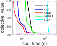
(a) a1a.

(b) a9a.

Figure 1: Objective vs CPU time (logscale) on two data sets.

Figure 2: The progress of residual value $\left\|X_{k}-Y_{k}\right\|_{F}^{2}$ on a9a.

5.2 Results on CMVU

Two benchmark data sets, USPS Digits and Newsgroups 20 are used in our experiments, and their information can be referred to (Song et al., 2008). As in (Song et al., 2008), we construct the set ${\mathcal{N}}$ by considering the $1\%$ nearest neighbors of each point. The tradeoff parameter $\lambda$ is set to $1$ as a default. The problem dimensionality $n$ is straightly set as the number of all data points.

Figure 3 shows the convergences of the objective on the USPS Digits and Newsgroups 20 data sets respectively. It can be observed that, to arrive the final objective-value (a broken mauve line), AAGD converges faster than the others. On these two data sets, the run time of SQLP exceeds $5000$ seconds, so we don’t plot them.

(a) USPS Digits.

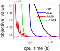
(b) Newsgroups 20.

Figure 3: Objective vs CPU time (logscale) on the USPS Digits and Newsgroups 20.

6 Conclusion

Many problems in machine learning can be reduced to SDP formulation, but existing SDP solvers by classical convex optimization are expensive to solve large-scale problems. PSD constraint is the most challenging aspect of solving SDP. In order to overcome this difficulty, Burer-Monteiro’s method reformulated SDP as a nonconvex problem via the quadratic factorization. However, this would lose the structure of problem in optimization. Different from Burer-Monteiro method, we propose to convert SDP into a biconvex program via the bilinear factorization, with the addition of a Courant penalty. We show that, if the condition of rank deficiency is satisfied, a local minimizer of the biconvex surrogate will provide a global minimizer of the original SDP problem when the penalty parameter is larger than a theoretical bound. Our proposal can be easily optimized using alternating accelerated gradient descent algorithm. Experiments on two SDP-related problems demonstrate that the proposed algorithm is scalable.

For the future, we would generalize the biconvex surrogate for SDP to more complex circumstances. For example, we can combine biconvex structure to the (augmented) Lagrangian schem for constrained SDP program. Additionally, we will consider the second-order optimize for the proposed biconvex problem.

Appendix A PROOFS

A.1 Proof of Proposition 1

Proof.

Let $\alpha_{1},\alpha_{2}\geq 0$, $\alpha_{1}+\alpha_{2}=1$ and $\forall Y,X_{1},X_{2}\in{\mathbb{R}}^{n\times r}$, according to the definition of $f$ in (4) we have

$$f\left((\alpha_{1}X_{1}+\alpha_{2}X2),Y\right) = \dot{f}\left((\alpha_{1}X_{1}+\alpha_{2}X2)Y^{\top}\right)$$

$$= \dot{f}\left(\alpha_{1}X_{1}Y{{}^{\top}}+\alpha_{2}X_{2}Y{{}^{\top}}\right)$$

$$\leq \alpha_{1}\dot{f}(X_{1}Y{{}^{\top}})+\alpha_{2}\dot{f}(X_{2}Y{{}^{\top}})$$

$$= \alpha_{1}f\left(X_{1},Y\right)+\alpha_{2}f\left(X_{2},Y\right)$$

where the first and last equalities use the definition of $f(\cdot,\cdot)$ in (4), and the inequality uses convexity of $\dot{f}(\cdot)$, so we conclude that $f(X,\cdot)$ is convex. Similarly we can conclude that $f(\cdot,Y)$ is convex. Hence, $f(\cdot,\cdot)$ is biconvex. As ${\gamma\over 2}\left\|X-Y\right\|_{F}^{2}$ is biconvex, $F(X,Y;\gamma)$ in (3) is biconvex. ∎

A.2 Proof of Theorem 1

Proof.

By contradiction, assume ${\bar{X}}\neq{\bar{Y}}$ when $\gamma>\frac{1}{4}(L-\sigma)_{+}$. Since $({\bar{X}},{\bar{Y}})$ is a stationary point of (3), we have

$$\text{tr}[({\bar{Y}}-{\bar{X}}){{}^{\top}}\nabla_{1}F({\bar{X}},{\bar{Y}};\gamma)]=0,$$ (24)

$$\text{tr}[({\bar{X}}-{\bar{Y}}){{}^{\top}}\nabla_{2}F({\bar{X}},{\bar{Y}};\gamma)]=0.$$ (25)

Expand the above and use biconvexity, we have

$$\gamma\left\|{\bar{Y}}-{\bar{X}}\right\|_{F}^{2} = \text{tr}[({\bar{Y}}-{\bar{X}})^{\top}\nabla_{1}f({\bar{X}},{\bar{Y}})\leq f({\bar{Y}},{\bar{Y}})-f({\bar{X}},{\bar{Y}})$$ (26)

$$\gamma\left\|{\bar{X}}-{\bar{Y}}\right\|_{F}^{2} = \text{tr}[({\bar{X}}-{\bar{Y}})^{\top}\nabla_{2}f({\bar{X}},{\bar{Y}})]\leq f({\bar{X}},{\bar{X}})-f({\bar{X}},{\bar{Y}}).$$ (27)

Add this two inequalities, we have

$$\gamma \leq \frac{f({\bar{Y}},{\bar{Y}})-f({\bar{X}},{\bar{Y}})+f({\bar{X}},{\bar{X}})-f({\bar{X}},{\bar{Y}})}{2\left\|{\bar{Y}}-{\bar{X}}\right\|_{F}^{2}}$$ (28)

$$\leq \frac{\text{tr}[\nabla_{1}f({\bar{Y}},{\bar{Y}}){{}^{\top}}({\bar{Y}}-{\bar{X}})+\nabla_{2}f({\bar{X}},{\bar{X}}){{}^{\top}}({\bar{X}}-{\bar{Y}})]}{2\left\|{\bar{Y}}-{\bar{X}}\right\|_{F}^{2}}-\frac{\sigma}{2}$$

$$= \frac{\text{tr}[(\nabla_{1}f({\bar{Y}},{\bar{Y}})-\nabla_{2}f({\bar{X}},{\bar{X}})){{}^{\top}}({\bar{Y}}-{\bar{X}})]}{2\left\|{\bar{Y}}-{\bar{X}}\right\|_{F}^{2}}-\frac{\sigma}{2}$$

$$= \frac{\text{tr}[(2\nabla_{1}f({\bar{Y}},{\bar{Y}})-2\nabla_{2}f({\bar{X}},{\bar{X}})){{}^{\top}}({\bar{Y}}-{\bar{X}})]}{4\left\|{\bar{Y}}-{\bar{X}}\right\|_{F}^{2}}-\frac{\sigma}{2}$$

$$= \frac{\text{tr}[(\nabla\ddot{f}({\bar{Y}})-\nabla\ddot{f}({\bar{X}})){{}^{\top}}({\bar{Y}}-{\bar{X}})]}{4\left\|{\bar{Y}}-{\bar{X}}\right\|_{F}^{2}}-\frac{\sigma}{2}$$

$$\leq \frac{L\left\|{\bar{Y}}-{\bar{X}}\right\|_{F}^{2}}{4\left\|{\bar{Y}}-{\bar{X}}\right\|_{F}^{2}}-\frac{\sigma}{2}$$

$$\leq \frac{1}{4}(L-\sigma)_{+}.$$

The first inequality comes from (26)$\sim$(27), the second inequality uses the $\sigma$-strong biconvexity of $f(X,\cdot)$ and $f(\cdot,Y)$ in (7)$\sim$(8) and the third inequality uses (6) in Assumption 2. The last equality uses (9). Thus $\gamma\leq\frac{1}{4}(L-\sigma)_{+}$ in (28) contradicts with the starting assumption $\gamma>\frac{1}{4}(L-\sigma)_{+}$.

∎

A.3 Proof of Corollary 1

Proof.

The condition of Theorem 1 holds, $({\bar{X}},{\bar{Y}})$ is a stationary point of $F$ implies that ${\bar{X}}={\bar{Y}}$.

1. From $f(X,Y)=\dot{f}(XY^{\top})$ in (4), we have the Fréchet derivative of $f$ in term of $X$ as

   $$\nabla_{1}f(X,Y) = \nabla\dot{f}(Z)\Big{|}_{Z=XY^{\top}}Y.$$ (29)

   From (9), the Fréchet derivative of $\ddot{f}$ in (2) is

   $$\nabla\ddot{f}(X) = 2\nabla\dot{f}(Z)\Big{|}_{Z=XX^{\top}}X.$$ (30)

   As that $({\bar{X}},{\bar{Y}})$ is a stationary point of $F(X,Y;\gamma)$ and ${\bar{X}}={\bar{Y}}$, we have

   $$\nabla_{1}F({\bar{X}},{\bar{Y}};\gamma)\Big{|}_{{\bar{Y}}={\bar{X}}}=0$$

   $$\Rightarrow [\nabla_{1}f({\bar{X}},{\bar{Y}})+\gamma({\bar{X}}-{\bar{Y}})]\Big{|}_{{\bar{Y}}={\bar{X}}}=0$$

   $$\Rightarrow \nabla_{1}f({\bar{X}},{\bar{X}})=0$$

   $$\Rightarrow \nabla\dot{f}({\bar{Z}})\Big{|}_{{\bar{Z}}={\bar{X}}{\bar{X}}^{\top}}{\bar{X}}=0$$

   $$\Rightarrow \frac{1}{2}\nabla\ddot{f}({\bar{X}})=0$$

   $$\Rightarrow \nabla\ddot{f}({\bar{X}})=0,$$

   where the fourth equality uses (29) and the fifth equality uses (30) respectively. The above implies that ${\bar{X}}$ is a stationary point of $F$.

2. If $({\bar{X}},{\bar{Y}})$ is a local minimizer of $F(X,Y;\gamma)$, we have

   $$F({\bar{X}},{\bar{Y}};\gamma)\leq F({\bar{X}}+\varTheta,{\bar{Y}}+\varTheta;\gamma),\forall\varTheta\in\{\varTheta\Big{|}\varTheta\in{\mathbb{R}}^{n\times r},\left\|\varTheta\right\|_{F}\longrightarrow 0\}.$$ (31)

   When the condition of Theorem 1 is satisfied, we have ${\bar{X}}={\bar{Y}}$, so that

   $$F({\bar{X}},{\bar{Y}};\gamma)=f({\bar{X}},{\bar{Y}})=\dot{f}({\bar{X}}{\bar{X}}^{\top}),F({\bar{X}}+\varTheta,{\bar{Y}}+\varTheta;\gamma)=\dot{f}(({\bar{X}}+\varTheta)({\bar{X}}+\varTheta)^{\top}).$$ (32)

   Combining (31) and (32), we have

   $$\ddot{f}({\bar{X}})=\dot{f}({\bar{X}}{\bar{X}}^{\top})\leq\dot{f}(({\bar{X}}+\varTheta)({\bar{X}}+\varTheta)^{\top})=\ddot{f}({\bar{X}}+\varTheta).$$

   The last inequality means that ${\bar{X}}$ is a local minimizer of $\ddot{f}(X)$.

∎

A.4 Proof of Proposition 2

Proof.

Specified to (15) and (16), we compute $\tau_{k}^{X}$ and $\tau_{k}^{Y}$ in Algorithm 1 respectively.

1. Computing the optimal stepsize $\tau^{X}_{k}$

   Let $\hat{d}=\nabla_{1}F(\hat{X}_{k-1},Y_{k-1};\gamma_{\frac{k}{2}})$, we have

   $$X_{k} = \hat{X}_{k-1}-\tau_{k}^{X}\nabla_{1}F(\hat{X}_{k-1},Y_{k-1};\gamma_{\frac{k}{2}})$$

   $$= \hat{X}_{k-1}-\tau_{k}^{X}\hat{d}$$

   in step 6 of Algorithm 1.

   So, the optimal $\tau_{k}^{X}$ is the solution of following problem

   $$\tau_{k}^{X} = \operatorname{arg\,min}\limits_{\tau\geq 0}:F(\hat{X}_{k-1}-\tau\hat{d},Y_{k-1};\gamma_{\frac{k}{2}})$$

   $$= \operatorname{arg\,min}\limits_{\tau\geq 0}:\frac{1}{2}{\rm{vec}}(\hat{X}_{k-1}-\tau\hat{d})^{\top}{\mathcal{A}}^{Y}_{k}{\rm{vec}}(\hat{X}_{k-1}-\tau\hat{d})-{\rm{vec}}(\hat{X}_{k-1}-\tau\hat{d})^{\top}{\textit{b}}^{Y}_{k}+constant$$

   $$= \operatorname{arg\,min}\limits_{\tau\geq 0}:\frac{1}{2}[{\rm{vec}}(\hat{d})^{\top}{\mathcal{A}}^{Y}_{k}{\rm{vec}}(\hat{d})]\tau^{2}-[{\rm{vec}}(\hat{d})^{\top}({\mathcal{A}}^{Y}_{k}{\rm{vec}}(\hat{X}_{k-1})-{\textit{b}}^{Y}_{k})]\tau+constant$$

   $$= \frac{{\rm{vec}}(\hat{d})^{\top}({\mathcal{A}}^{Y}_{k}{\rm{vec}}(\hat{X}_{k-1})-{\textit{b}}^{Y}_{k})}{{\rm{vec}}(\hat{d})^{\top}{\mathcal{A}}^{Y}_{k}{\rm{vec}}(\hat{d})}$$

   $$= \frac{{\rm{vec}}(\hat{d})^{\top}{\rm{vec}}(\nabla_{1}F(\hat{X}_{k-1},Y_{k-1};\gamma_{\frac{k}{2}}))}{{\rm{vec}}(\hat{d})^{\top}{\mathcal{A}}^{Y}_{k}{\rm{vec}}(\hat{d})}$$

   $$= \frac{{\rm{vec}}(\hat{d})^{\top}{\rm{vec}}(\hat{d})}{{\rm{vec}}(\hat{d})^{\top}{\mathcal{A}}^{Y}_{k}{\rm{vec}}(\hat{d})}$$

   $$= \frac{\left\|\hat{d}\right\|_{F}^{2}}{{\rm{vec}}(\hat{d})^{\top}{\mathcal{A}}^{Y}_{k}{\rm{vec}}(\hat{d})}$$

   $$= \frac{\left\|d^{X}_{k}\right\|_{F}^{2}}{{d^{X}_{k}}^{\top}{\mathcal{A}}^{Y}_{k}d^{X}_{k}}$$

   where the last fourth equality uses ${\mathcal{A}}^{Y}_{k}{\rm{vec}}(\hat{X}_{k-1})-{\textit{b}}^{Y}_{k}={\rm{vec}}(\nabla_{1}F(\hat{X}_{k-1},Y_{k-1};\gamma_{\frac{k}{2}}))$, which can be obtained from (15), the last third equality uses $\hat{d}=\nabla_{1}F(\hat{X}_{k-1},Y_{k-1};\gamma_{\frac{k}{2}})$, the last first equality uses ${\rm{vec}}(\hat{d})={\rm{vec}}(\nabla_{1}F(\hat{X}_{k-1},Y_{k-1};\gamma_{\frac{k}{2}}))=d^{X}_{k}$ defined in (22).

2. Computing the optimal stepsize $\tau^{Y}_{k}$ is similar to $\tau^{X}_{k}$.

∎

References

• Aksoylar et al. [2017] Cem Aksoylar, Lorenzo Orecchia, and Venkatesh Saligrama. Connected subgraph detection with mirror descent on SDPs. In ICML, pages 51–59, 2017.
• Beck and Teboulle [2009] A. Beck and M. Teboulle. A fast iterative shrinkage-thresholding algorithm for linear inverse problems. SIJIS, 2(1):183–202, 2009.
• Burer and Choi [2006] S. Burer and C. Choi. Computational enhancements in low-rank semidefinite programming. Optimization Methods and Software, 21(3):493–512, 2006.
• Burer and Monteiro [2003] S. Burer and R.D.C. Monteiro. A nonlinear programming algorithm for solving semidefinite programs via low-rank factorization. MathProg, 95:329–357, 2003.
• D’aspremont et al. [2007] A. D’aspremont, El L. Ghaoui, M. I. Jordan, and G. R. G. Lanckriet. A direct formulation for sparse PCA using semidefinite programming. SIAM Review, 49(3):434–48, 2007.
• Erdogdu et al. [2017] Murat A. Erdogdu, Yash Deshpande, and Andrea Montanari. Inference in graphical models via semidefinite programming hierarchies. In NeurIPS, pages 416–424, 2017.
• Frank and Wolfe [1956] Marguerite Frank and Philip Wolfe. An algorithm for quadratic programming. Naval Research Logistics, 3:149–154, 1956.
• Ge et al. [2017] Rong Ge, Chi Jin, and Yi Zheng. No spurious local minima in nonconvex low rank problems: A unified geometric analysis. In ICML, pages 1233–1242, 2017.
• Ghadimi and Lan [2016] Saeed Ghadimi and Guanghui Lan. Accelerated gradient methods for nonconvex nonlinear and stochastic programming. Mathematical Programming, 156(1-2):59–99, 2016.
• Hu et al. [2011] E.-L. Hu, B. Wang, and S.-C. Chen. BCDNPKL: Scalable non-parametric kernel learning using block coordinate descent. In ICML, pages 209–216, 2011.
• Jaggi [2013] M. Jaggi. Revisiting Frank-Wolfe: Projection-free sparse convex optimization. In ICML, 2013.
• Journeé et al. [2010] M. Journeé, F. Bach, P.A. Absil, and R. Sepulchre. Low-rank optimization on the cone of positive semidefinite matrices. SIOPT, pages 2327–2351, 2010.
• Laue [2012] S. Laue. A hybrid algorithm for convex semidefinite optimization. In ICML, pages 177–184, 2012.
• Li and Lin [2015] H. Li and Z. Lin. Accelerated proximal gradient methods for nonconvex programming. In NeurIPS, pages 379–387, 2015.
• Li and Tang [2017] Q.W. Li and G.G. Tang. The nonconvex geometry of low-rank matrix optimizations with general objective functions. In GlobalSIP, 2017.
• Nesterov and Nemirovski [1994] Y. Nesterov and A. Nemirovski. Interior-Point Polynomial Algorithms in Convex Programming. SIAM, 1994.
• Nocedal and Wright [2006] J. Nocedal and S.J. Wright. Numerical Optimization. Springer, 2006.
• Obozinski et al. [2009] G. Obozinski, B. Taskar, and M. I. Jordan. Joint covariate selection and joint subspace selection for multiple classification problems. Statistics and Computing, 20(2):231–252, 2009.
• Rand [1971] W. M. Rand. Objective criteria for the evaluation of clustering methods. Journal of the American Statistical Association, 66:846–850, 1971.
• Royer [2017] M. Royer. Adaptive clustering through semidefinite programming. In NeurIPS, pages 1793–1801, 2017.
• Song et al. [2008] L. Song, A. Smola, K. Borgwardt, and A. Gretton. Colored maximum variance unfolding. In NeurIPS, 2008.
• Srebro et al. [2005] N. Srebro, J.D.M. Rennie, and T.S. Jaakola. Maximum-margin matrix factorization. In NeurIPS 17, pages 1329–1336, 2005.
• Srinadh et al. [2016] B. Srinadh, K. Anastasios, and Sujay S. Dropping convexity for faster semidefinite optimization. In Conference on Learning Theory, 2016.
• Tropp et al. [2017] Joel A Tropp, Alp Yurtsever, Madeleine Udell, and Volkan Cevher. Fixed-rank approximation of a positive-semidefinite matrix from streaming data. In NeurIPS 30, pages 1225–1234, 2017.
• Weinberger et al. [2004] K. Q. Weinberger, F. Sha, and L.K. Saul. Learning a kernel matrix for nonlinear dimensionality reduction. In ICML, pages 839–846, 2004.
• Wu et al. [2009] X.-M. Wu, A. M.-C. So, Z. Li, and S.-Y.R. Li. Fast graph Laplacian regularized kernel learning via semidefinite-quadratic-linear programming. In NeurIPS 22, pages 1964–1972, 2009.
• Xing et al. [2002] E. Xing, A. Ng, M. Jordan, and S. Russell. Distance metric learning with application to clustering with side-information. In NeurIPS, pages 505–512, 2002.
• Xu and Yin [2013] Y. Xu and W. Yin. A block coordinate descent method for regularized multiconvex optimization with applications to nonnegative tensor factorization and completion. SIAM Journal on Imaging Sciences, 6(3):1758–1789, 2013.
• Zheng and Lafferty [2015] Q. Zheng and J. Lafferty. A convergent gradient descent algorithm for rank minimization and semidefinite programming from random linear measurements. In NeurIPS, 2015.
• Zhuang et al. [2011] J. Zhuang, I. Tsang, and S. Hoi. A family of simple non-parametric kernel learning algorithms. JMLR, 12:1313–1347, 2011.