Pushing the boundaries of audiovisual word recognition using Residual Networks and LSTMs

Abstract

Visual and audiovisual speech recognition are witnessing a renaissance which is largely due to the advent of deep learning methods. In this paper, we present a deep learning architecture for lipreading and audiovisual word recognition, which combines Residual Networks equipped with spatiotemporal input layers and Bidirectional LSTMs. The lipreading architecture attains 11.92% misclassification rate on the challenging Lipreading-In-The-Wild database, which is composed of excerpts from BBC-TV, each containing one of the 500 target words. Audiovisual experiments are performed using both intermediate and late integration, as well as several types and levels of environmental noise, and notable improvements over the audio-only network are reported, even in the case of clean speech. A further analysis on the utility of target word boundaries is provided, as well as on the capacity of the network in modeling the linguistic context of the target word. Finally, we examine difficult word pairs and discuss how visual information helps towards attaining higher recognition accuracy.

1 Introduction

Audiovisual automatic speech recognition (ASR) is the problem of recognizing speech by combining audio and video information. It is well known that auditory perception can be profoundly modified by visual information for the speaker’s lip movements (McGurk and MacDonald, 1976; MacDonald and McGurk, 1978).

In the past decades, several approaches for integrating visual information in ASR systems were introduced. Most of them were based on encoding visual information with handcrafted features or statistical shape models (e.g. active shape models) and modeling the sequence of hidden states and the emission probability of each state (Potamianos et al., 2003) with continuous density hidden-Markov models (HMMs). Despite their limitations, such as the controlled environments and the poor generalizability to speakers unseen during training, those systems demonstrated the efficacy of visual information in improving the ASR accuracy especially in noisy environments. More recently, the tremendous progress witnessed in audio-based ASR and computer vision due to deep learning methods, together with the release of large, publicly available and “in-the-wild” audiovisual databases have refreshed the interest in audiovisual ASR. Deep learning methods originally introduced in audio-only ASR are combined with computer vision models (e.g. convolutional neural networks, CNNs) and achieve vast improvements in recognition accuracy even in unconstrained videos (Chung et al., 2017).

In this article, we introduce an audiovisual architecture which goes beyond state-of-the-art in visual and audiovisual word recognition. We focus on the Lipreading-In-The-Wild (LRW) database, which is the largest publicly available database for the task (Chung and Zisserman, 2016, 2018). The evaluation protocol is closed-set word identification, where each video contains one of the 500 target words. However, target words are not isolated, but appear within phrases, which are excerpted from BBC-TV and are of fixed duration (1.16s). Moreover, word boundaries indicating the beginning and the end of each target word are given (Chung and Zisserman, 2016).

Our lipreading architecture is composed of a Residual Network (ResNet) with spatiotemporal (3D) input layers and a Bidirectional LSTM (BiLSTM) backend. We explore several configurations, the best of which attains 11.92% misclassification rate (MCR). Our audio architecture is based entirely on BiLSTM, it uses plain log-spectral features and it is designed in such a way so that it can be naturally integrated with the lipreading network. Contrary to typical stacks of BiLSTMs, where the two directional outputs are concatenate after every BiLSTM layer, we concatenate them only at last BiLSTM layer. To examine the gain in performance under noisy conditions, we use the DEMAND dataset, which contains several types of environmental noise. The performance of the audiovisual system is compared to the audio-only system under different SNR levels, as well as to score-level fusion (i.e. late integration (Katsaggelos et al., 2015)). Moreover, we examine word confusion between challenging word pairs and we show how visual information helps towards reducing it.

LRW is a recently released database and one of its main properties is that target words appear within utterances with given target word boundaries. Therefore, a thorough experimentation on the optimal use of target word boundaries and on the way the network may utilize the context of the target word is worth to be conducted. To this end, we first examine ways of exploiting the word boundaries and we show that passing them as indicator variables yields substantially superior results compared to using them in order to remove frames preceding or succeeding the target word (out-of-boundaries frames), as proposed in Chung and Zisserman (2018). Moreover, we test whether this improvement is due to an implicit modeling of the linguistic context of the target word. By training and evaluating a network entirely on out-of-boundaries frames, we show that a small fraction of target words can be recognized using merely their context.

The rest of the paper is organized as follows. In Section 2 we present some of the recent works in lipreading and audiovisual speech recognition, while in Section 3 we give a description of the “Lipreading-In-The-Wild” database. In Section 4 we describe our lipreading architecture while the audio and audiovisual architectures are discussed in Section 5. In Section 6 we present experiments using several lipreading architectures and configurations, followed by audio and audiovisual experiments in Section 7. In Section 8 we provide a further analysis on the results, e.g. by focusing on difficult word pairs and trying to quantify the contribution of the word context in the results. Finally, conclusions and further applications of the proposed ResNet features and training scheme are discussed in Section 9.

2 Related work

Research on visual speech recognition witnessed a first wave of interest few decades ago, either as a stand-alone application or as a means to enhance audio-only ASR (Zhou et al., 2014). Traditional visual ASR systems typically deploy an appearance or shape-based feature extractor, a set of linear or nonlinear transforms for suppressing the undesired variability associated to speaker, pose, or other sources, and an HMM with which transitions between visemes are modeled. Visemes are defined as the set of static or dynamic mouth shapes representing clusters of contrastive phonemes (e.g. /p, b, m/, and /f, v/) (Taylor et al., 2012). Appearance-based visual features are typically derived by applying PCA, discrete cosine transform (DCT), or discrete wavelet transform (DWT) on the region of interest, while shape-based features model the contours of the speaker’s lips, via geometric descriptors or statistical models of shape, such as active shape models (Dalton et al., 1996; Luettin and Thacker, 1997; Chan, 2001). Common ASR transforms such as Linear Discriminant Analysis (LDA) and feature-space Maximum Likelihood Linear Regression (fMLLR) are also applied to visual features, in order to enhance their discriminability and to adapt them to the speaker’s characteristics (Potamianos and Neti, 2003). Active appearance models (AAM), i.e. generative models for the shape and the texture of faces (and objects in general) have also been very effective in visual and audiovisual ASR. Apart from their appealing properties as features which combine shape and texture information, they offer a principled way for dynamically estimating the visual feature observation uncertainty, allowing for uncertainly-aware HMM training and fully adaptive audiovisual integration schemes (Papandreou et al., 2009; Matthews et al., 2002).

Over the past few years, a new wave of visual and audiovisual ASR architectures has been observed, which are largely inspired by advances in deep learning and especially those emerged in audio-only ASR and computer vision. The use of Recurrent Neural Networks (RNNs) was first explored in Wand et al. (2016), where Long Short-Term Memory (LSTM) networks are applied to the GRID corpus. The proposed network is speaker dependent, as a result of the small speaker variability in GRID which makes generalizability to new speakers hard. A speaker independent extension of the network is proposed in Wand and Schmidhuber (2017), where features are mapped to a common speaker independent space using domain adversarial neural networks (Ganin and Lempitsky, 2015). In Assael et al. (2016) LipNet is introduced, a system which combines Convolutional Neural Networks (CNNs) and Gated Recurrent Units (GRUs), capable of performing sentence-level recognition on GRID. The lack of frame-level annotation is addressed by Connectionist Temporal Classification (CTC, Graves et al. (2006)), which together with attentive sequence-to-sequence neural networks are the two dominant approaches in end-to-end ASR (Hori et al., 2017). LipNet is also the first lipreading model to employ spatiotemporal convolutions in the input layers. In Koumparoulis et al. (2017) the authors propose the use of convolutional LSTMs with skip connections and perform experiments on the IBM audiovisual database of connected digits. The proposed architecture combines the strength of LSTMs in sequence modeling with the efficacy of spatial convolutions in a unified model. The authors report drastic improvements over conventional GMM-HMM based systems with handcrafted features (Potamianos and Neti, 2003). In Chung and Zisserman (2018), the research team which collected “Lipreading-In-The-Wild” improves its previous architecture (Chung and Zisserman, 2016) by combining a VGG network with an LSTM backend. The improved architecture attains 36.0% WER, which is further reduced to 29.5% when the target word boundaries are used to discard out-of-boundaries frames. Very recently, an improvement of the LipNet is introduced in Shillingford et al. (2018). A deep architecture comprising spatiotemporal convolutions, BiLSTMs, phoneme-distributions and CTC loss is trained on a new large-scale database for lipreading. The authors report 40.9% WER, outperforming LipNet and attentive encoder-decoder architectures (Chung et al., 2017) by a large margin. Finally, in Afouras et al. (2018a), the authors propose a lipreading system deploying self-attention layers (Transformer network) (Vaswani et al., 2017). The experiments show that it yields better results compared to architectures with convolutional and BiLSTM-based backends.

In parallel, research in integrated audiovisual ASR architectures is moving towards deep learning end-to-end methods. In audiovisual ASR, intermediate and late integration (or fusion) are the two main approaches deployed to combine the two modalities. Intermediate integration refers to those approaches having modality-specific front-ends, with the two modalities being merged in the backend of the audiovisual architecture. On the other hand, in late integration, two separate systems are trained and their probabilistic outputs are combined, by applying a weighted average over the logarithmic likelihoods or posterior probabilities (Katsaggelos et al., 2015). Hybrid approaches exist as well, such as architectures where the two modalities are merged at the decision level with a bilinear layer, enabling joint bi-modal training (Mroueh et al., 2015), or approaches using gating layer to reduce the effect of noisy or uninformative visual features (Tao and Busso, 2018). In Petridis et al. (2017), the authors propose an end-to-end intermediate integration architecture with fully connected layers in the frontend and a single-layer BiLSTM in the backend. The results reported on OuluVS2 database demonstrate a notable improvement over the audio-only version of the architecture, when the Signal-to-Noise Ratio (SNR) is $\leq$15dB (Anina et al., 2015). In Mroueh et al. (2015), audiovisual architectures with fully connected layers in the frontend and three different integration approaches are compared. The first architecture is a intermediate integration approach, where the two modalities are concatenated in the feature space and passed as input to a Deep Neural Network (DNN). The second is a late fusion approach, where the scores are averaged on the log-posterior domain, while the third is a hybrid approach where merging is performed by a factored bilinear SoftMax layer. The experimental results performed on the IBM AV-ASR Large Vocabulary Studio Dataset show that the first two approaches perform equally well and clearly better that the third one. Finally, in Chung et al. (2017), an end-to-end audiovisual architecture is proposed, which expands the “Listen, Attend and Spell” audio-only ASR approach to visual and audiovisual ASR (Chan et al., 2016). The architecture is based on sequence-to-sequence models (also known as encoder-decoder) with attention. Intermediate integration is performed by the speller (i.e. the decoder), whose estimates are conditioned on two context vectors, one for each modality. The system is evaluated on the Lipreading Sentences in-the-wild (LRS) database, which is the second large and in-the-wild audiovisual database made available recently (Chung et al., 2017). Apart from the experiments on LRS, the authors conduct experiments with a lipreading version of their architecture on GRID (attaining the best published results) as well as on LRW.

3 The Lipreading-In-The-Wild database

LRW is the largest publicly available audiovisual database for word-level audiovisual speech recognition. It is composed of short videos from BBC news and talk-shows, excerpted using a pipeline for fully automated large-scale data collection from TV broadcasts (Chung and Zisserman, 2016). It is characterized by high variability in speakers, motion and resolution, as well as by a large number of target words and training instances per word. Pose variability is clearly higher compared to other datasets (e.g. GRID), although views are in general between $0^{\circ}$ and $30^{\circ}$. Due to its large training set, training deep architectures from scratch is feasible, using standard data augmentation (e.g. random crops, horizontal flips) and regularization methods (e.g. dropouts, batch normalization). The main statistics and characteristics of LRW are summarized in Table 1.

There are several word pairs with small pairwise edit distance, such as MILLION-BILLION, SPEND-SPENT, RUSSIA-RUSSIAN, BENEFIT-BENEFITS. Moreover, the target words occupy the central frames of the utterance, making word recognition even more challenging due to co-articulation with preceding and succeeding words. Target word boundaries are given for all splits (training, development and test) and algorithms may use them to localize the target words. Finally, the faces are registered and therefore the region of interest (mouth region) can be extracted directly using fixed cropping for all frames and videos, without applying face detection and facial landmark detection and tracking. Fig. 1 depicts a sequence of frames from an LRW video corresponding to the word EVERYTHING (frames lying out of the word boundaries are not depicted). The region of interest is defined similarly to Chung et al. (2017), i.e. it is square and relatively wide.

Table 1: LRW database statistics and characteristics

Target words	500
Training instances	488766
Development instances	25000
Test instances	25000
Training instances per word	800 - 1000
Range of views	$0^{\circ}$ - $30^{\circ}$
Video duration	1.16s
Frames per video	29
Speakers	$>$1000

Fig. 1: Frame sequence from LRW, corresponding to the word EVERYTHING. Frames are cropped as those we use as input to the lipreading network.

4 Lipreading Network

In this section, we focus on the visual part on the network. The network can be naturally partitioned into a frontend and a backend. The frontend is a modified 18-layer Residual Network, while the backend is a 2-layer BiLSTM, modeling the probability of the input sequence containing each target word.

4.1 Frontend: ResNet with spatiotemporal input layers

We use an $18$-layer ResNet, which we found to performing equally well with the 34-layer we used in Stafylakis and Tzimiropoulos (2017). ResNets are convolutional networks with skip connections, which facilitate training of deep architectures (He et al., 2016). They can be decomposed into 4 different blocks, each reducing the spatial size while increasing the number of channels by a factor of 2. We make two modifications on the ResNet to make it more effective for the particular task. (a) We replace the first spatial (i.e. 2D) layers with their spatiotemporal (i.e. 3D) analogues (Tran et al., 2015; Ji et al., 2013). The first convolutional layer has kernel size of $64\times 5\times 7\times 7$ (channels$\times$time$\times$width$\times$height), while max pooling has a kernel size equal to $1\times 1\times 3\times 3$. At this stage, we do not reduce the time resolution, therefore we set the temporal stride equal to $1$. (b) We replace the average pooling layer of the ResNet output by a fully connected layer. The average pooling layer is more adequate for problems requiring translation invariance (e.g. object recognition and detection) but it is less justified for images of the mouth region. The block of layers transform the tensors as $1\times 112\times 112\rightarrow 64\times 28\times 28\rightarrow 128\times 14\times 14\rightarrow 256\times 7\times 7\rightarrow 512\times 4\times 4$ (channels$\times$width$\times$height), while the last set of layers transforms them as $512\times 4\times 4\rightarrow 8192\times 1\times 1\rightarrow 256\times 1\times 1$ (the temporal dimension is suppressed for clarity and its size is fixed, $T^{V}=29$).

4.2 Backend I: Temporal convolutional

The first backend we deploy is a temporal convolutional network. It is a rather simple backend, the main purpose of which is to initialize the ResNet (we did not succeed in training from scratch the architecture with BiLSTM backend). Its building blocks are composed of a temporal convolutional layer, followed by batch normalization, Rectified Linear Units (ReLU) and temporal max pooling. Each of the two layers reduces the time resolution by a factor of $4$ (by using a stride equal to $2$ in the convolutional and max pooling layers), while the number of channels is increased by $2$. The tensor sizes (time$\times$channels) are therefore $29\times 256\rightarrow 7\times 512\rightarrow 1\times 1024$. The final linear layers implement a bottleneck $1024\rightarrow 256\rightarrow 500$, followed by a SoftMax layer to approximate the posterior probability over the $N_{w}=500$ target words.

4.3 Backend II: Bidirectional LSTMs

Our proposed backend is composed of a two-layer BiLSTM (without peepholes) of $256$-size, followed by an average pooling layer which aggregates information across time-steps, a fully connected (FC) linear and a SoftMax layer. Our two-layer BiLSTM differs from the usual stack of two BiLSTM layers; we obtained significantly better results by concatenating the two directional outputs only at the output of the second LSTMs. The backend receives as input the collection of $256$-size features extracted by the ResNet, augmented by a binary variable indicating whether or not the frame lies inside or outside the word boundaries, i.e.

$$\mathbf{x}^{+}_{t}=\left[\mathbf{x}_{t},b_{t}\right],$$ (1)

where

$$\mathbf{x}_{t}=\mbox{ResNet}(D_{v})_{t}$$ (2)

is the $t$-th output of the ResNet, $D_{v}$ is the collection of frames and

$$b_{t}=\mathbbm{1}_{t\in B}$$ (3)

is the indicator variable denoting whether $t$-th frame lies within the word boundaries $B$.

The BiLSTM layers are followed by an average pooling layer, which aggregates temporal information into a fixed length representation. We apply dropouts with $p=0.30$ to the inputs of each LSTM (yet not to the recurrent layer, see Cheng et al. (2017)). Following the theoretical justification in Gal and Ghahramani (2016), a single mask is sampled and applied to all frames of a given sequence. Finally, batch normalization is applied to the average pooling layer, together with a dropout layer with $p=0.15$ (Ioffe and Szegedy, 2015).

Fig. 2: The block-diagram of the lipreading network with BiLSTM backend. Tensor sizes correspond to the output tensors of each module. Inputs are depicted with blue, trainable components of the network with orange, and non-trainable components with green.

4.4 Training algorithm, optimization and evaluation

We train the network by using the cross entropy criterion over word labels with ADAM optimizer (Kingma and Ba, 2014). The initial learning rate is equal to $3\times 10^{-3}$, the final is equal to $10^{-5}$, and we reduce it by a factor of 2 when no progress is attained on the validation set after 3 consecutive epochs. We evaluate the performance using the argmax operator, i.e.

$$\hat{w}=\operatorname*{argmax}_{w}p(w|D_{v},\Theta_{v}).$$ (4)

where $\Theta_{v}$ is the set of parameters of the visual network, $D_{v}$ is a frame sequence, and $w\in\cal{W}$ is a word of the vocabulary of target words $\cal{W}$, where $\left|\cal{W}\right|=N_{w}=500$.

5 Audio and Audiovisual Networks

In this section, our architecture for audio-based speech recognition is introduced and discussed, together with intermediate and late audiovisual integration.

5.1 Proposed architecture for audio-only word recognition

Contrary to the visual network, the audio network is based entirely on BiLSTMs, which have demonstrated an enormous capacity in audio-only ASR (Sak et al., 2014; Chan et al., 2016). We use a deep 4-layer BiLSTM architecture with the two directions being concatenated only at the output of the final LSTMs (similarly to the backend on the lipreading network). The audio is modeled using 161-dimensional log-spectral features, extracted at 100fps frame rate, i.e. 4 times the visual frame rate. We compensate for this difference by adding a subsampling layer to the output of the first two BiLSTMs, each dropping the frame rate by a factor of 2. As a result, the sequence of audio features which is passed to the backend has 25fps frame rate. There are at least two approaches to implement this reduction in the audio frame rate. The first is to subsample the LSTM output vectors used as input to the next layer, e.g. to pass only the even frames to the next LSTM. The second is via frame concatenation. In this latter case, we concatenate two consecutive LSTM output vectors and use them as input to the subsequent LSTM layer. This approach is often called pyramidal LSTM (pLSTM) and has shown its efficacy when combined with the attentive encoder-decoder architecture for audio-only ASR introduced in Chan et al. (2016). The standard LSTM equation (ignoring the internal mechanism) is as follows

$$\mathbf{h}_{t}^{l}=\mbox{LSTM}(\mathbf{h}_{t-1}^{l},\mathbf{h}_{t}^{l-1}),$$ (5)

where $l$ and $t$ denote LSTM layer and time index, respectively, while $\mathbf{h}_{t}^{l}$ is the output vector of the LSTM. The pLSTM is as follows

$$\mathbf{h}_{t}^{l}=\mbox{pLSTM}(\mathbf{h}_{t-1}^{l},\left[\mathbf{h}_{2t}^{l-1},\mathbf{h}_{2t+1}^{l-1}\right]),$$ (6)

where $\left[\cdot,\cdot\right]$ denotes vector concatenation. Similarly to the lipreading network, word boundaries are passed to the network as a sequence of binary indicator variables, which are concatenated with the spectral features. We apply batch normalization to the input of each LSTM as well as dropouts. The architecture is illustrated in Fig. 3. We denote by $T^{A}$ the number of audio input frames, where $T^{A}=4\times T^{V}=116$ in LRW.

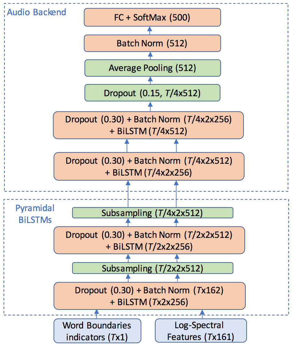
Fig. 3: The block-diagram of the audio network. Pyramidal are the two BiLSTM which are followed by a subsampling layer. $T$ corresponds to the set of audio features, i.e. $T=T^{A}=116$.

Audio features are extracted every 10ms with a sliding window of 20ms. The resulting 161-sized features are normalized with respect to mean and variance, with statistics estimated from the whole utterance. Note that the statistics are common to all frequency bins, i.e. a scalar mean and variance is estimated from and applied to all 161 bins. Estimating robust statistics for each frequency bin is hard for two reasons. First, the duration of the utterances is very short (1.16sec). Second, we use plain log-spectral features, and therefore we do not average over neighboring frequency bins as in the case of MFCC and filterbank features.

5.2 Audiovisual architectures and integration

Our first audiovisual architecture follows intermediate integration and is derived by merging the audio and lipreading networks in the backend. As Fig. 2 and Fig. 3 show, the two networks share the same backend and frame rate, and we can therefore unify them by concatenating the frontend outputs. The way we concatenate the audio with the visual frontend is shown in the lower part of Fig. 4. We observe that audio, visual and word boundaries sequences are concatenated separately in each of the two directions, while the concatenation is taking place at the output of the two front-ends. This is slightly different compared to the audio-only network, where word boundaries sequences are concatenated directly with spectral features sequences.

For regularization, we deploy a version of multimodal training method suggested in Chung et al. (2017). More specifically, we randomly drop either the audio or the visual frame sequence, each with probability $0.25$, i.e. $p_{d}^{A}=p_{d}^{V}=0.25$. Moreover, we drop the word boundaries indicator variables with probability $p_{d}^{W}=0.25$. Multimodal training is a special case of dropout regularization, where a single binary variable is sampled for each sequence of audio, video and word boundaries indicator variables. Moreover, sampling is dependent for the two modalities, so that the probability of dropping both modalities is equal to 0, while the probability of keeping both modalities is equal to $0.50$.

Note that due to the lower frame rate and the spatiotemporal input layers, visual features span a wide context window. More specifically the visual context window is equal to $5\times 40$ms = $200$ms, where 5 corresponds to the temporal size of the ResNet. Hence, for the concatenation to be meaningful, the acoustic features should have a wide context window, too. The 2-layer pyramidal BiLSTM (pBiLSTM) acoustic frontend is by construction capable of extracting features spanning wide time windows. Therefore, apart from the requirement of reducing the audio frame rate by a factor of 4, the further requirement of extracting acoustic features with sufficiently wide context window is a further rationale for deploying the particular 2-layer pBiLSTM acoustic frontend.

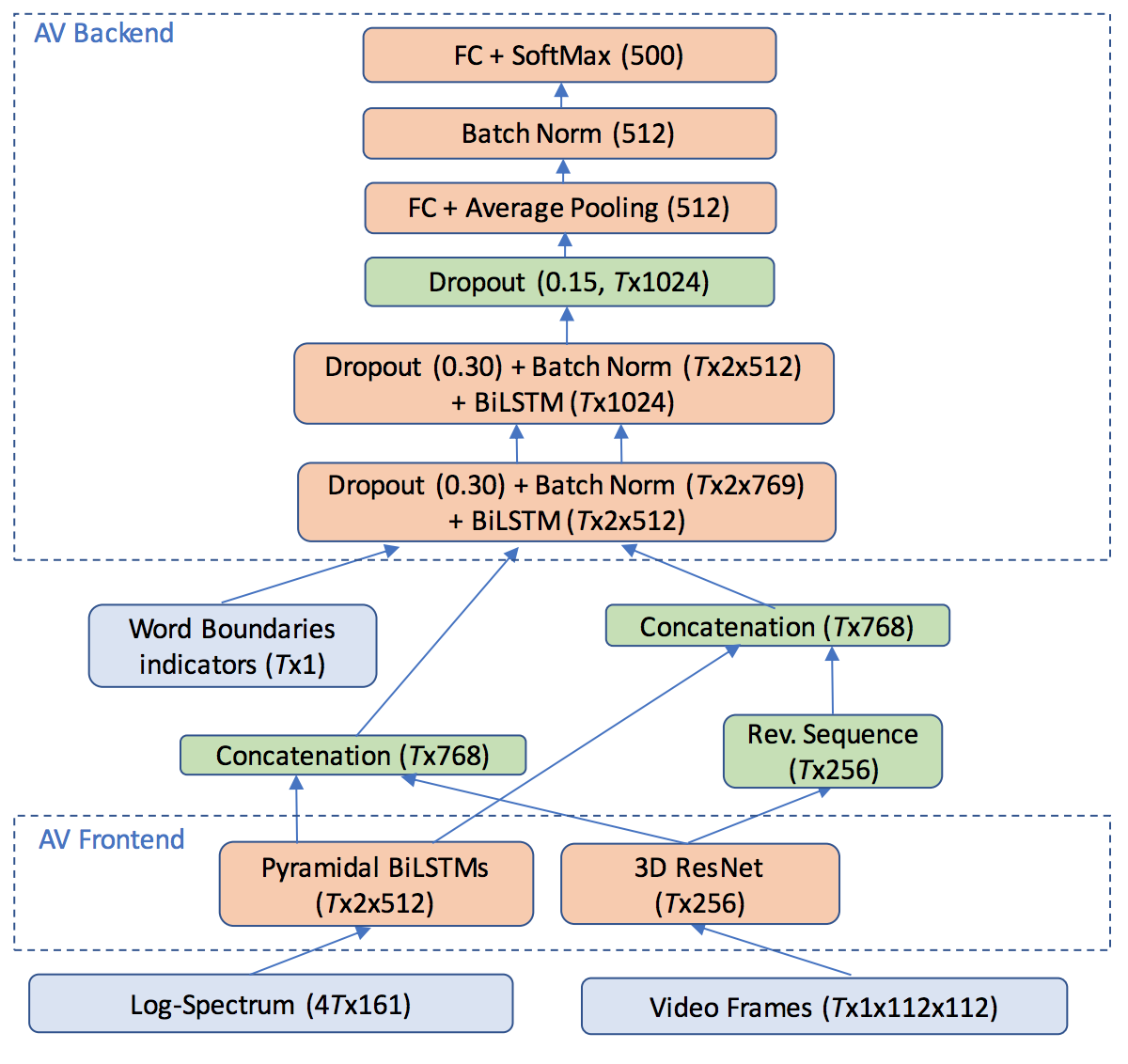
Fig. 4: The block-diagram of the audiovisual network. $T$ corresponds to the set of video frames, i.e. $T=T^{V}=29$.

Apart from intermediate integration, we also experiment with late integration. In this case, two unimodal systems are trained independently and the output of the audiovisual system is calculated as the weighted sum of the log-posteriors, which is equivalent to

$$p(w|D_{a},D_{v},\Theta_{a},\Theta_{v})\propto p(w|D_{v},\Theta_{v})^{\gamma}p(w|D_{a},\Theta_{a})^{1-\gamma},$$ (7)

and the decision is based on

$$\hat{w}=\operatorname*{argmax}_{w}p(w|D_{a},D_{v},\Theta_{a},\Theta_{v}).$$ (8)

The weight of the visual system is $\gamma=0.40$, which we optimized on a noisy version of the validation set.

6 Lipreading experiments

In this section, we report experimental results with our lipreading system. We start by presenting the baseline and the current state-of-the-art on LRW, followed by experiments using the temporal convolutional backend and optical flow. Results using the proposed system will follow, together with different configurations of the LSTM backend. Finally, the effectiveness of the proposed way of using the word boundaries will be examined and compared to the conventional approach of out-of-boundaries frame removal.

6.1 Baseline and state-of-the-art

As baseline system we consider the architecture introduced in Chung et al. (2017) called “Watch, Attend and Spell” (WAS). It is essentially an encoder-decoder network with temporal attention, using characters as recognition units, and it is a visual extension of the “Listen, Attend and Spell” audio-only ASR network introduced in Chan et al. (2016). The architecture is capable of performing sentence-level recognition, scoring 50.2% Word Error Rate (WER) on the “Lipreading Sentences in-the-wild” database. It is worth-mentioning that a professional lipreader scored 73.8% on the same dataset, underlining the efficacy of the proposed architecture and training algorithm. The architecture was fine-tuned on the LRW training set and evaluated on its test set yielding $23.80\%$ MCR (Table 2, WAS). The state-of-the-art in LRW is introduced by our research team in (Stafylakis and Tzimiropoulos, 2017) and its differences with the proposed architecture have been discussed in Section 4. The network attains 17.03% MCR in LRW (Table 2, ResNet-BiLSTM).

Table 2: Lipreading baseline and state-of-the-art results on LRW. VGG-M/LSTM is reported in Chung and Zisserman (2018), Watch, Attend and Spell in Chung et al. (2017), while ResNet/BiLSTM in Stafylakis and Tzimiropoulos (2017).

System	MCR (%)
VGG-M/LSTM	28.50
Watch, Attend and Spell	23.80
ResNet/BiLSTM	17.03

6.2 Lipreading architectures: frontend, ResNet and backend

In the first set of experiments, we present a set of results which are useful in assessing the contribution of each module. We begin with the temporal convolutional backend and we compare a network having spatial (i.e. 2D) or spatiotemporal (i.e. 3D) input layers (denoted by V1 and V2 in Table 3). Clearly, the contribution of the 3D input layers is significant, yielding 4.66% absolute improvement. Note that the optimal temporal kernel size (equal to 5) is determined after experimentation, where we observed no gains by increasing it further. Similar conclusions about the efficacy of a spatiotemporal input layers can be found in Assael et al. (2016), where they are combined with GRUs in the backend. To determine the size of the ResNet we include an experiment (denoted by V3) using a 34-layer ResNet, as we suggested in our previous work (Stafylakis and Tzimiropoulos, 2017). Comparing V2 and V3 we conclude that 18-layer ResNet yields better results and it is the one we proceed with, given also its fewer parameters (about 2/3 of those in 34-ResNet). In the next experiment, we aim to assess the contribution of the fully connected layer over the baseline average pooling. We argue that average pooling is more relevant to domains where invariance towards translations is required (e.g. object recognition and detection), but it is less justifiable in the domain we examined, where the mouth region is aligned at each frame. The architecture where average pooling is replaced by a fully connected linear layer is denoted by V4. We observe a notable improvement, which demonstrates the effectiveness of a learnable layer over a fixed spatial averaging. The best results in this set of experiments are obtained when BiLSTMs are used in the backend. Network V6 combines a spatiotemporal 18-layer ResNet with BiLSTM backend and attains 17.01% MCR.

A question worth-posing is whether the spatiotemporal input layers are still required even when BiLSTMs are deployed. To address it, we train a network with 2D ResNet and BiLSTMs (denoted by V5). By comparing its performance to that of V6 we observe that the spatiotemporal input layers are highly beneficial even with BiLSTM backend, yielding 6.27% absolute improvement over V5. In other words, spatial ResNet features, even when combined with powerful RNN models are incapable of competing with spatiotemporal ResNet features in modeling the motion patterns of the mouth region. The reason is that temporal correlations should be modeled over fine-grained spatial information, and the latter is not preserved in spatial ResNet features.

Table 3: Lipreading results with various network configurations. Comparisons: 2D vs 3D: spatial vs spatiotemporal layers in the frontend (FE), 18 vs 34: number of convolutional layers in ResNet, AP vs FC: Average pooling vs fully connected layer for eliminating the spatial dimensions in the ResNet. TConv vs BiLSTM: Temporal convolutional vs BiLSTM backend (BE).

Net	FE	ResNet	Pooling	BE	MCR (%)
V1	2D	18	AP	TConv	29.37
V2	3D	18	AP	TConv	24.71
V3	3D	34	AP	TConv	25.44
V4	3D	18	FC	TConv	22.51
V5	2D	18	FC	BiLSTM	23.28
V6	3D	18	FC	BiLSTM	17.01

6.3 Lipreading architectures with optical flow

In this section we investigate the use of optical flow as input feature, either alone or together with frames. Optical flow is a two-dimensional vector field indicating the motion of each individual pixel between two successive frames (Black and Anandan, 1993). It has been extensively used in action recognition as well as in lipreading, usually combined with frames (Simonyan and Zisserman, 2014; Shiraishi and Saitoh, 2015). To experiment with it, we extract the optical flow for each frame and we treat each of its two dimensions as a channel, either alone (i.e. $2\times 112\times 112$ input tensor size) or together with the (grayscale) frame (i.e. $3\times 112\times 112$ input tensor size). We perform experiments with the ResNet-18 and the temporal convolutional backend. The results are given in Table 4. Interestingly, none of the four configurations yield superior results compared to using frames alone. The architectures using spatiotemporal input layers (V8 and V10) perform again better compared to those using spatial ones (V7 and V9). Although other configurations may be considered for using optical flow (e.g. by using intermediate integration (Simonyan and Zisserman, 2014)), we conclude that the spatiotemporal input layers operating on frames can model temporal information sufficiently well. Therefore, for the rest of our experiments optical flow will not be included.

Table 4: Lipreading results with optical flow features. Comparisons: 2D vs 3D: spatial vs spatiotemporal input layers in the frontend (FE), Optical Flow vs Frames: indicated whether optical flow and regular frames are used as input.

Net	FE	Optical Flow	Frames	MCR (%)
V7	2D	✓		37.79
V8	3D	✓		34.68
V9	2D	✓	✓	39.44
V10	3D	✓	✓	30.28

6.4 Our lipreading architecture with BiLSTM backend

For the next set of experiments we fix the frontend obtained by the V6 network and use it to extract and store ResNet features, which will be used for the rest of our experiments. Working directly with ResNet features instead of video frames enables us to train several backend configurations on a single GPU using up to 100 epochs, each within 1-2 days. Note that pre-trained ResNet networks in Torch7 and PyTorch and the code for training and evaluating them are available. Moreover, we found no notable gains in performance by training the networks end-to-end, as long as the ResNet features are extracted with a network trained with BiLSTM backend, such as V6.

Having fixed the main building blocks of our architectures, we perform experiments in order to improve the backend. We experiment with regularization methods (dropouts and batch normalization), number of BiLSTM layers, as well as with using the last time step of BiLSTM output to aggregate temporal information, as in Wand et al. (2016). Word boundaries are included in all the experiments of this section in the form of binary indicator variables, as shown in Fig. 2.

In the first experiment we include dropouts in the backend. The results are given in Table 5 (denoted by V11) and the network attains $13.65$% MCR. For the second experiment (denoted by V12) we add batch normalization without dropouts to the backend. The MCR the network attained is $14.52$%, showing the batch normalization alone is less effective compared to dropouts. In the next configuration we use both dropouts and batch normalization, but a single BiLSTM layer. The network, denoted by V13, attains $13.04$% MCR, showing that combining dropouts with batch normalization yields good results even with a single BiLSTM layer. In the next configuration (denoted by V14) we use the last time step to aggregate temporal information instead of average pooling. By using this method (proposed e.g. in Wand et al. (2016)) and combining it with dropouts, batch normalization and a 2-layer BiLSTM, the network attains $12.15$% error rate. The final architecture we examine is the one shown in Fig. 2 and it is denoted by V15. Its sole difference from V14 is the use of average pooling to aggregate information across time steps. Its attains $11.92$% MCR, which is the best visual-only results we attain and corresponds to half the MCR attained by the baseline system (Table 2). We should also mention that we experimented with the typical stacking approach of BiLSTM. In this case, the outputs of the first BiLSTM are concatenated and used as input to the second BiLSTM. The network failed to attain good results (error rates above $20$%), despite our efforts to tune parameters such as learning rate and dropout probabilities.

Table 5: Lipreading results for various network configurations. Abbreviations: #L: number of BiLSTM layers, DO: use of dropouts at the backend, BN: use of batch normalization after average pooling, TA: temporal aggregation using average pooling (A) or using the last time step (L).

Net	#L	DO	BN	TA	MCR (%)
V11	2	✓		A	13.65
V12	2		✓	A	14.52
V13	1	✓	✓	A	13.04
V14	2	✓	✓	L	12.15
V15	2	✓	✓	A	11.92

6.5 Experimentation on the use of word boundaries

How effective is the proposed method of using word boundaries as indicators variables and how it compares to other ways of using them? To address this question, we first retrain the backend without passing the word boundaries. The system yields 15.7% MCR, as Table 6 shows. This result is interesting in two ways; first of all, it is substantially inferior to the one attained by V15, demonstrating the utility of using word boundaries. Secondly, it is clearly superior to the current state-of-the-art (17.03% MCR, Table 2) demonstrating the gain in performance attained by the improved architecture. We also compare our method with the conventional approach of removing those frames lying out of word boundaries. In this case, the backend is trained with sequences of ResNet features of variable length. The MCR attained by this approach is 14.94% (V17, Table 6) which corresponds to a modest absolute improvement of 0.8% over a network that does not use word boundaries (i.e. V16).

Table 6: Lipreading results on the utility of word boundaries.

Net	Word Boundaries	MCR (%)
V15	Indicator variables	11.92
V16	Not used	15.67
V17	Frame removal	14.94

Several hypotheses can be postulated from this set of experiments. First of all, LSTMs have a powerful gating mechanism and the technique of passing the word boundaries as an additional feature permits the LSTM to make use of them. Furthermore, LSTMs are capable of modeling long-range temporal dependencies, such as those related to the characteristics of the particular utterance (e.g. speaker, pose, and other utterance-level characteristics). Hence, the out-of-boundaries frames can be used by the BiLSTM backend to model such dependencies (by accumulating relevant information in the cell), and apply essentially a fast and coarse adaptation to the input ResNet features of the particular utterance, before the target-word frames arrive. Finally, the out-of-boundaries frames carry information about the linguistic context of the target word, which might be useful for identifying the target word. A further set of experiments on the utility of out-of-boundaries frames is presented in Section 8.

The results obtained by V17 (i.e. using frame removal) can be compared to those reported in Chung and Zisserman (2018) using frame removal, LSTMs and a VGG-M frontend. As Table 2 shows, their architecture attains 28.50% MCR, which is about twice the MCR obtained by the V17. This drastic improvement in performance can be attributed to the 3D-ResNet, as the other ingredients of the two networks as very similar.

For convenience, we list all the visual-only networks we examined and the corresponding MCRs in Table 11.

7 Audio and Audiovisual Experiments

In this section, we provide experimental results attained by incorporating the audio modality in the architecture. In the first part of the section we provide details about the experimental set-up and the use of noise to make the audiovisual problem more challenging. After some first experiments where the audio modality is used alone, we explore the proposed audiovisual architectural variants and report their performance under different noisy conditions.

7.1 Audio Experiments

7.1.1 Noise database and multi-condition training

LRW is not a noise-free database as it is composed of real-world recordings from BBC-TV. On the other hand, an additional noise database is required in order to perform controlled experiments under different noisy environments and noise levels. To this end, we make use of the publicly available Diverse Environments Multichannel Acoustic Noise Database (DEMAND (Thiemann et al., 2013)). The database contains 18 different types of background noise (noisy environments), which are partitioned into 6 categories: domestic, nature, office, public, street and transportation. Each type is recorded using a 16-channel microphone array, resulting in 16 different audio files for each of the 18 environments (i.e. 288 audio files overall).

We use the first 4 categories for training, while testing is performed on all 6 categories. Each audio file is randomly chosen from a uniform distribution, and the same holds for the time interval from which noise is extracted. Moreover, to further enrich the noisy environments we include combinations of noises, namely noise mixtures composed of $N_{n}=\{0,1,2,3\}$ audio files, where $N_{n}$ is sampled from a uniform distribution, and $N_{n}=0$ corresponds to recordings without additive noise. The noise level of all noise types is uniformly distributed between -12dB to 22dB SNR, including the noise mixtures. For testing, we use fixed noisy audio files, so that each network is scored against identical test sets. Noise is sampled and added following a similar procedure with which we train the network, with two differences: (a) We do not consider mixtures of noises, and (b) we create one noisy set from all the test set of LRW, each corresponding to a predefined noise level: -10dB to 20dB SNR with 5dB step as well as on speech without additive noise. The addition of the noise takes place on the waveform domain.

7.1.2 Audio results without additive noise

In Table 7 we present results on LRW recordings without additive noise. We test again the use of word boundaries, either as indicator variables (A3 and A4), or for removing out-of-boundaries frames (A2). We observe again the superiority of the former approach over the latter. Moreover, applying frame removal hurts recognition accuracy even when compared to not using word boundaries at all (A1).

We moreover examine an alternative approach for performing subsampling, where we keep every odd output of the first two LSTMs instead of concatenating odd and even outputs. The network, denoted by A3, yields a slight increase in MCR compared to A4, indicating the superiority of pBiLSTM approach over simpler subsampling approaches. Finally, it is also worth examining whether the reduction of the frame rate causes any degradation in performance. To this end, we train an audio-only network (denoted by A5) which does not apply any frame rate reduction. It is similar to A4 but uses standard BiLSTMs instead of pBiLSTMs. Interestingly, we observe a slight degradation compared to A4, which shows that the use of pBiLSTMs is not harmful for the accuracy obtained by the audio component.

Table 7: Audio results on recordings without additive noise. WB: Word Boundaries, FR: Frame Rate at the output of the second pyramidal BiLSTM. The results show that the combination of pyramidal BiLSTMs with WB used as indicator variable yields the best performance.

Net	Fr. Concat.	WB	FR	MCR (%)
A1	✓	Not used	25fps	2.04
A2	✓	Fr. removal	25fps	2.08
A3		Indicat. Var.	25fps	1.52
A4	✓	Indicat. Var.	25fps	1.38
A5		Indicat. Var.	100fps	1.45

7.2 Audiovisual experiments

In this section we present the results using audiovisual architectures and we compare them to our best audio-only architecture (A4). We perform experiments with 4 audiovisual networks; the first (denoted by AV1) is a intermediate integration network, the second (denoted by AV2) has the same architecture with AV1 but it is trained with multimodal training (i.e. by randomly dropping audio and video modalities as well as word boundaries, a technique inspired by Chung et al. (2017)), the third (denoted by AV3) is the same as AV2 but without word boundaries, and finally the fourth (AV4) is a late integration system of our best performing audio (A4) and video (V15) networks (i.e. with word boundaries). In AV4, the weights of the video and audio networks are $\gamma$ and $1-\gamma$, respectively, where $\gamma=0.40$.

Table 8: Audio and audiovisual results on noisy recordings. The noise level is between -10dB and 20dB and the DEMAND noise database is used. The results show (a) the vast increase in performance attained by incorporating visual information, (b) the effectiveness of multimodal training, and (c) the gap in performance between intermediate and late integration.

Net	Integration	Multimodal	WB	MCR (%)
A4	-	-	✓	6.90
AV1	Intermediate		✓	2.79
AV2	Intermediate	✓	✓	2.20
AV3	Intermediate	✓		3.17
AV4	Late		✓	1.90

The results in Table 8 demonstrate the huge improvement attained by including the visual component in noisy environments. Relative improvement equal to 72.4% is attained by using late integration over the audio-only network. Moreover, in intermediate integration we observe the large improvement from applying multimodal training, suggested in Chung et al. (2017). Clearly, though, late integration performs better than intermediate, which is in line with other works on audiovisual integration, such as Mroueh et al. (2015). We conclude that more effort is required to make intermediate integration performing better than late, and methods such as multimodal training are very helpful towards this direction. Finally, AV3 is useful (a) for quantifying the contribution of word boundaries, yielding about 30% relative improvement in terms of MCR, and (b) for comparing our architecture with other recently proposed audiovisual architectures that do not make use of word boundaries, such as Petridis et al. (2018).

8 Error analysis

In this section we present a detailed analysis of the results attained by our best architectures. More specifically, we break down the errors by noise category and SNR, we demonstrate how well each architecture performs on difficult word pairs and we examine to which extent the linguistic context of the target word is helping towards higher recognition accuracy.

8.1 Error rates for each noise level and category

In Section 7.2 we reported results averaged over 7 different noise levels and 6 different categories. We provide here a more detailed analysis, by breaking down the error rates by noise category and noise level. In Fig. 5 we present MCR attained by 5 architectures, where each MCR is derived as the average over all noise categories (i.e. 6 $\times$ 25000 = 150000 videos). Although the relative improvement attained by audiovisual architectures is larger under extreme noisy conditions (-10dB to -5dB), notable improvements are attained even in higher SNRs (0dB to 20dB) as well as on speech without additive noise. Moreover, by comparing the MCR of our best visual-only network (V15) with our best audio-only network (A4) we conclude that the performance of the former is equivalent to that of the latter with $\textrm{SNR}\approx-4.5$ additive noise.

Fig. 5: MCR for audio and three audiovisual networks using DEMAND noise database (25dB correspond to speech without additive noise).

Similarly, in Fig. 6 we report results for each noise category of the DEMAND noise database. The results are averaged across all 7 noise levels. We observe a high variability in the error rates between noise categories. The category “public” is the most challenging (also known as babble noise), probably due to the high spectral overlap between noise and clean speech. Interestingly, “street” and “transportation” do not yield worse results than “domestic”, “nature” or “office”, despite the fact that the former two are not included in training.

Fig. 6: MCR on the 6 noise categories of DEMAND (Domestic, Nature, Office, Public, Street and Transportation) averaged across all 7 noise SNR levels.

8.2 Challenging Word Pairs

As there are many word pairs in LRW with similar phonetic content, it is interesting to examine the error rates attained by each architecture on such pairs. We select the most challenging pairs based on the performance of the audio-only network (A4) at 10dB and noise category “public” (babble noise). The list of word pairs with the highest confusion is given in Table 9, together with the corresponding number of occurrences (recall there are 50 videos for each target word). The number of errors made by the proposed lipreading network (V15) on the same set of pairs is also given. Finally, we report the number of errors made by the audiovisual systems AV2 and AV4.

Table 9 provides some insight regarding the way visual information assists audio-only word recognition. For instance, visual representation of phoneme /b/ in the word BORDER enhances its discriminability from the word ORDER. The words SERIES and SERIOUS have lower mutual confusion in the audiovisual setting, due to the visual information in phoneme /ah/. Similarly, visual differences between phonemes /r/ and /m/ assist discrimination between words RIGHT and MIGHT. As a final example, visual information in phoneme /f/ helps to discriminate between words STAFF and START. For a thorough analysis of mappings between phonemes and visemes (i.e. visual analogues of phonemes) in lipreading we refer to Bear et al. (2014).

8.3 Word recognition using only the context

As a final experiment, we aim to assess the extent to which the linguistic context helps towards recognizing the target words. The experiments on the various ways word boundaries may be utilized ($3\%$ difference in MCR between V15 and V17, Table 6) indicate that out-of-boundaries frames carry useful information for word identification. However, the way the network utilizes this information is unclear. One possibility is that the backend is using out-of-boundaries frames for a coarse utterance and speaker adaptation, while a second one is that it models the linguistic context of the target word. Hence, a question worth-posing is whether or not it is possible to recognize the target words given only its context.

Table 9: Word pairs exhibiting the highest confusion when the audio-only network is used (A4), and how visual information reduces the error rates, using either intermediate (AV2) or late integration (AV4, $\gamma=0.40$). The number of test examples is 50 per word and the SNR is 10dB (DEMAND dataset).

Word Pairs		#Errors/Net
Target	Estimated	A4	V15	AV2	AV4
WHETHER	WEATHER	10	2	3	5
THERE	THEIR	8	6	8	8
SPENT	SPEND	8	9	5	6
THEIR	THERE	6	6	7	6
HAPPENED	HAPPEN	5	4	5	3
WEATHER	WHETHER	5	2	2	2
STATE	STATES	5	0	2	2
CALLED	COURT	5	6	3	3
TAKING	TAKEN	4	5	3	3
SERIES	SERIOUS	4	7	4	2
ORDER	BORDER	4	0	0	0
AMERICAN	AMERICA	4	10	3	3
STAGE	STATE	3	1	1	3
STAFF	START	3	3	0	1
SCHOOL	SCHOOLS	3	1	3	3
THROUGH	THREE	3	2	1	1
SERIOUS	SERIES	3	4	2	0
MONTHS	MONTH	3	2	1	2
SPEND	SPENT	3	13	5	4
ELECTION	ACTION	3	1	3	2
THINK	THING	3	5	4	5
HAPPEN	HAPPENED	3	2	2	2
RIGHT	MIGHT	3	0	0	1
START	STAFF	2	0	0	1

To this end, we train a lipreading system using only out-of-boundaries frames. The network (which we denote by V18) is the dual of V17 in the sense that the within-boundaries frames are now the ones being removed. The performance of V18 is $88.86\%$ MCR, which is significantly better compared to random selection, i.e. $1-1/500=99.80\%$ MCR. Moreover, we observe certain words on which the network performs reasonably well ($\leq 50\%$ MCR), listed in Table 10. A common characteristic of most of these words is that they are frequently preceded or succeeded by few others, such as “David CAMERON”, “Northern IRELAND”, “PRIME minister”, i.e. the probability of observing them given their linguistic context is relatively high. We conclude that the network is using all available frames to create an implicit language model which helps towards distinguishing between two or more target words having similar phonetic/visemic content. This property can at least partly explain the gains in performance attained by keeping out-of-boundaries frames.

Finally, the ability of the proposed architecture to discriminate even between homophones (WHETHER vs. WEATHER) should also be linked to the use of words as main recognition units (rather than visemes, phonemes and other sub-word units). The proposed architecture, when presented with a large number of training examples seems capable of capturing certain differences in the way homophones are expressed within phrases, which cannot be captured by systems that use visemes as main recognition units (since the two sequences of visemes are identical), unless a language model is applied.

Table 10: 15 words which can be recognized fairly well using only out-of-boundaries frames ($\leq 50\%$ MCR). V18: Lipreading network trained and evaluated using only out-of-boundaries frames. V15: Our best lipreading system that uses all frames.

MCR (%)
Word	V18	V15
CAMERON	20	2
IRELAND	24	2
EDITOR	32	14
PRIME	36	2
UNION	38	2
ISLAMIC	38	0
SUNSHINE	42	0
NORTHERN	44	4
MINISTER	44	2
GEORGE	44	24
SIDES	44	20
AFFAIRS	44	14
AFTERNOON	46	4
DAVID	48	8
WINDS	50	2

9 Conclusions and further applications

In this paper we introduced a deep architecture for audiovisual word recognition. The architecture is trained and evaluated on “Lipreading in the wild” (LRW), a recently released audiovisual database composed of short excerpts from BBC-TV. LRW has several appealing characteristics, such as large variability in speakers, motion and resolution, and large number of target words and training instances per word, permitting training of deep end-to-end architectures without pertained models.

In the first part of the paper we focused on the lipreading network, where we examined several network options, regarding the use of spatiotemporal input layers in the ResNet, the size of the ResNet and the use of optical flow. The main conclusions we draw are that (a) the proposed frontend yields substantial improvement over the standard spatial ResNet, even with BiLSTM backend, (b) optical flow is not useful at least in early integration with frames, (c) there is no gain by using a 34-layer ResNet over an 18-layer one, and (d) BiLSTMs are performing much better compared to simple temporal convolutions in the backend. After fixing the architecture of the frontend, we turned our focus to the backend, where we experimented with BiLSTMs and regularization methods, as well as with method of using the word boundaries. The experiments show among others that (a) combining dropouts and batch normalization yields notably improved results, and (b) passing the word boundaries as additional binary indicator features yields substantial improvement over removing out-of-boundaries frames.

For the audio part of the network, we proposed a deep BiLSTM network using log-spectrum as input. The backend of the audio network is identical to the visual, so that they can be merged into a single audiovisual architecture. To this end, the first two BiLSTM layers apply subsampling in their outputs, reducing the audio frame fate from 100fps to 25fps. The audio network is trained using noisy inputs, with noise samples drawn from the DEMAND database. Experiments on audio without additive noise demonstrated the capacity of the network in addressing word recognition and reaffirmed the efficacy of the method by which we make use of word boundaries. On the other hard, experiments on noisy audio showed the drastic performance degradation of audio-only ASR systems, especially when SNR $\leq$ 0dB. Furthermore, by breaking down the results by noise category, we show that babble noise (DEMAND category “public”) is the most difficult type to mitigate.

The experiments with audiovisual architectures indicated the vast improvements attained by combining the two modalities, either in the backend (intermediate integration) or in the score-domain (late integration). Intermediate integration, especially when random droppings on each modality and word boundaries are applied during training, yields results close -yet still inferior- to those attained by late integration. For noisy audio our best intermediate integration approach (AV2) yielded 2.20% compared to 1.90% attained by late integration, corresponding respectively to 68% and 72% relative improvement over the audio network alone (A4, 6.90% MCR). Furthermore, on speech without additive noise the two integration approaches attained relative improvement equal to 27% and 39% respectively, over the audio-only network. These results demonstrate the significant gains obtained by audiovisual integration even when without additive noise.

A final set of the experiments was conducted with the aim to explain the way by which the network utilizes out-of-boundaries frames. To quantify the capacity of the architecture in predicting the target word by its linguistic context we trained and evaluated a lipreading network only on out-of-boundaries frames. The results showed that there is a fraction of target words which can be predicted fairly well by their context alone; most of these words are frequently preceded or succeeded by a small set of other words (e.g. Northern IRELAND). This experiment indicates that the network makes use of the linguistic context of the target words to increase target-word recognition accuracy and provides a further rationale for our method of using target word boundaries as additional indicator variables.

We should finally emphasize that although the proposed networks were primarily designed to address the problem of closed-set word identification as defined by LRW, they are by no means restricted to it. The recently emerged acoustic-to-word family of models is capable of attaining state-of-the-art results in audio-only large vocabulary continuous speech recognition using words as recognition units, instead of the typical subword units such as collections of triphones (Li et al., 2018; Audhkhasi et al., 2017; Li et al., 2017). Visual keyword spotting is another application where words can be used as recognition units, and architectures deploying our ResNet as feature extractor (introduced in Stafylakis and Tzimiropoulos (2017)) have already shown very promising results (Stafylakis and Tzimiropoulos, 2018a, b; Jha et al., 2018). Moreover, there is evidence that the proposed training scheme (i.e. closed-set word identification on LRW with the aid of an LSTM backend) yields dynamic facial features attaining state-of-the-art performance on other tasks, which require fine-grained temporal information. Recent architectures for audiovisual speech enhancement and visual-only large vocabulary continuous speech recognition with characters as recognition units are such examples, where exceptional results are attained with our proposed ResNet features (Afouras et al., 2018b, a).

10 Acknowledgements

This project has received funding from the European Union’s Horizon 2020 research and innovation programme under the Marie Sklodowska-Curie grant agreement No 706668 (Talking Heads).

Table 11: List of visual-only networks

Net Input Features Word Boundaries ResNet Backend MCR (%) V1 Frames-2D - 18L-AP TConv 29.37 V2 Frames-3D - 18L-AP TConv 24.71 V3 Frames-3D - 34L-AP TConv 25.44 V4 Frames-3D - 18L-FC TConv 22.51 V5 Frames-2D - 18L-FC BiLSTM(x2) 23.28 V6 Frames-3D - 18L-FC BiLSTM(x2) 17.01 V7 Opt.Flow-2D - 18L-FC TConv 37.79 V8 Opt.Flow-3D - 18L-FC TConv 34.68 V9 Opt.Flow-Frames-2D - 18L-FC TConv 39.44 V10 Opt.Flow-Frames-3D - 18L-FC TConv 30.28 V11 Frames-3D Indicat. Var. 18L-FC BiLSTM(x2), w/o BN 13.65 V12 Frames-3D Indicat. Var. 18L-FC BiLSTM(x2), w/o DO 14.52 V13 Frames-3D Indicat. Var. 18L-FC BiLSTM(x1) 13.04 V14 Frames-3D Indicat. Var. 18L-FC BiLSTM(x2), Last Frame 12.15 V15 Frames-3D Indicat. Var. 18L-FC BiLSTM(x2) 11.92 V16 Frames-3D - 18L-FC BiLSTM(x2) 15.67 V17 Frames-3D Fr. Removal 18L-FC BiLSTM(x2) 14.94 V18 Frames-3D Within Bound. Fr. Removal 18L-FC BiLSTM(x2) 88.86

References

- Afouras et al. (2018a) Afouras, T., Chung, J.S., Zisserman, A., 2018a. Deep lip reading: a comparison of models and an online application, in: Interspeech.
- Afouras et al. (2018b) Afouras, T., Chung, J.S., Zisserman, A., 2018b. The Conversation: Deep Audio-Visual Speech Enhancement, in: Interspeech.
- Anina et al. (2015) Anina, I., Zhou, Z., Zhao, G., Pietikäinen, M., 2015. Ouluvs2: a multi-view audiovisual database for non-rigid mouth motion analysis, in: IEEE International Conference and Workshops on Automatic Face and Gesture Recognition (FG), pp. 1–5.
- Assael et al. (2016) Assael, Y.M., Shillingford, B., Whiteson, S., de Freitas, N., 2016. Lipnet: Sentence-level lipreading. arXiv preprint arXiv:1611.01599 .
- Audhkhasi et al. (2017) Audhkhasi, K., Ramabhadran, B., Saon, G., Picheny, M., Nahamoo, D., 2017. Direct acoustics-to-word models for english conversational speech recognition. arXiv preprint arXiv:1703.07754 .
- Bear et al. (2014) Bear, H.L., Harvey, R.W., Theobald, B.J., Lan, Y., 2014. Which phoneme-to-viseme maps best improve visual-only computer lip-reading?, in: International Symposium on Visual Computing, Springer. pp. 230–239.
- Black and Anandan (1993) Black, M.J., Anandan, P., 1993. A framework for the robust estimation of optical flow, in: International Conference on Computer Vision (ICCV), pp. 231–236.
- Chan (2001) Chan, M.T., 2001. Hmm-based audio-visual speech recognition integrating geometric- and appearance-based visual features, in: IEEE Fourth Workshop on Multimedia Signal Processing, pp. 9–14.
- Chan et al. (2016) Chan, W., Jaitly, N., Le, Q., Vinyals, O., 2016. Listen, attend and spell: A neural network for large vocabulary conversational speech recognition, in: IEEE International Conference on Acoustics, Speech and Signal Processing (ICASSP), pp. 4960–4964.
- Cheng et al. (2017) Cheng, G., Peddinti, V., Povey, D., Manohar, V., Khudanpur, S., Yan, Y., 2017. An exploration of dropout with LSTMs, in: Interspeech.
- Chung et al. (2017) Chung, J.S., Senior, A., Vinyals, O., Zisserman, A., 2017. Lip reading sentences in the wild, in: IEEE Conference on Computer Vision and Pattern Recognition (CVPR).
- Chung and Zisserman (2016) Chung, J.S., Zisserman, A., 2016. Lip reading in the wild, in: Asian Conference on Computer Vision (ACCV), Springer. pp. 87–103.
- Chung and Zisserman (2018) Chung, J.S., Zisserman, A., 2018. Learning to lip read words by watching videos. Computer Vision and Image Understanding .
- Dalton et al. (1996) Dalton, B., Kaucic, R., Blake, A., 1996. Automatic speechreading using dynamic contours, in: Speechreading by humans and machines. Springer, pp. 373–382.
- Gal and Ghahramani (2016) Gal, Y., Ghahramani, Z., 2016. A theoretically grounded application of dropout in recurrent neural networks, in: Advances in Neural Information Processing Systems (NIPS), pp. 1019–1027.
- Ganin and Lempitsky (2015) Ganin, Y., Lempitsky, V., 2015. Unsupervised domain adaptation by backpropagation, in: International Conference on Machine Learning (ICML), pp. 1180–1189.
- Graves et al. (2006) Graves, A., Fernández, S., Gomez, F., Schmidhuber, J., 2006. Connectionist temporal classification: labelling unsegmented sequence data with recurrent neural networks, in: Proceedings of the 23rd international conference on Machine learning (ICML), ACM. pp. 369–376.
- He et al. (2016) He, K., Zhang, X., Ren, S., Sun, J., 2016. Identity mappings in deep residual networks, in: European Conference on Computer Vision (ECCV), Springer. pp. 630–645.
- Hori et al. (2017) Hori, T., Watanabe, S., Zhang, Y., Chan, W., 2017. Advances in Joint CTC-Attention Based End-to-End Speech Recognition with a Deep CNN Encoder and RNN-LM, in: Interspeech.
- Ioffe and Szegedy (2015) Ioffe, S., Szegedy, C., 2015. Batch normalization: Accelerating deep network training by reducing internal covariate shift, in: International Conference on Machine Learning (ICML), pp. 448–456.
- Jha et al. (2018) Jha, A., Namboodiri, V., Jawahar, C., 2018. Word Spotting in Silent Lip Videos, in: Winter Conference on Applications of Computer Vision (WACV), 2018, IEEE.
- Ji et al. (2013) Ji, S., Xu, W., Yang, M., Yu, K., 2013. 3D convolutional neural networks for human action recognition. IEEE transactions on pattern analysis and machine intelligence 35, 221–231.
- Katsaggelos et al. (2015) Katsaggelos, A.K., Bahaadini, S., Molina, R., 2015. Audiovisual fusion: Challenges and new approaches. Proceedings of the IEEE 103, 1635–1653.
- Kingma and Ba (2014) Kingma, D.P., Ba, J., 2014. Adam: A Method for Stochastic Optimization, in: 3rd International Conference for Learning Representations (ICLR).
- Koumparoulis et al. (2017) Koumparoulis, A., Potamianos, G., Mroueh, Y., Rennie, S.J., 2017. Exploring ROI size in deep learning based lipreading, in: International Conference on Auditory-Visual Speech Processing (AVSP).
- Li et al. (2018) Li, J., Ye, G., Das, A., Zhao, R., Gong, Y., 2018. Advancing Acoustic-to-Word CTC Model. arXiv preprint arXiv:1803.05566 .
- Li et al. (2017) Li, J., Ye, G., Zhao, R., Droppo, J., Gong, Y., 2017. Acoustic-To-Word Model Without OOV. arXiv preprint arXiv:1711.10136 .
- Luettin and Thacker (1997) Luettin, J., Thacker, N.A., 1997. Speechreading using probabilistic models. Technical Report. IDIAP.
- MacDonald and McGurk (1978) MacDonald, J., McGurk, H., 1978. Visual influences on speech perception processes. Perception & Psychophysics 24, 253–257.
- Matthews et al. (2002) Matthews, I., Cootes, T.F., Bangham, J.A., Cox, S., Harvey, R., 2002. Extraction of visual features for lipreading. IEEE Transactions on Pattern Analysis and Machine Intelligence 24, 198–213.
- McGurk and MacDonald (1976) McGurk, H., MacDonald, J., 1976. Hearing lips and seeing voices. Nature 264, 746–748.
- Mroueh et al. (2015) Mroueh, Y., Marcheret, E., Goel, V., 2015. Deep multimodal learning for audio-visual speech recognition, in: International Conference on Acoustics, Speech and Signal Processing (ICASSP), pp. 2130–2134.
- Papandreou et al. (2009) Papandreou, G., Katsamanis, A., Pitsikalis, V., Maragos, P., 2009. Adaptive multimodal fusion by uncertainty compensation with application to audiovisual speech recognition. IEEE Transactions on Audio, Speech, and Language Processing 17, 423–435.
- Petridis et al. (2018) Petridis, S., Stafylakis, T., Ma, P., Cai, F., Tzimiropoulos, G., Pantic, M., 2018. End-to-end audiovisual speech recognition, in: IEEE International Conference on Acoustics, Speech and Signal Processing (ICASSP).
- Petridis et al. (2017) Petridis, S., Wang, Y., Li, Z., Pantic, M., 2017. End-to-end audiovisual fusion with lstms, in: International Conference on Auditory-Visual Speech Processing (AVSP).
- Potamianos and Neti (2003) Potamianos, G., Neti, C., 2003. Audio-visual speech recognition in challenging environments., in: Interspeech, pp. 1293–1296.
- Potamianos et al. (2003) Potamianos, G., Neti, C., Gravier, G., Garg, A., Senior, A.W., 2003. Recent advances in the automatic recognition of audiovisual speech. Proceedings of the IEEE 91, 1306–1326.
- Sak et al. (2014) Sak, H., Senior, A., Beaufays, F., 2014. Long short-term memory recurrent neural network architectures for large scale acoustic modeling, in: Interspeech.
- Shillingford et al. (2018) Shillingford, B., Assael, Y., Hoffman, M.W., Paine, T., Hughes, C., Prabhu, U., Liao, H., Sak, H., Rao, K., Bennett, L., et al., 2018. Large-Scale Visual Speech Recognition. arXiv preprint arXiv:1807.05162 .
- Shiraishi and Saitoh (2015) Shiraishi, J., Saitoh, T., 2015. Optical flow based lip reading using non rectangular roi and head motion reduction, in: IEEE International Conference and Workshops on Automatic Face and Gesture Recognition (FG), pp. 1–6.
- Simonyan and Zisserman (2014) Simonyan, K., Zisserman, A., 2014. Two-stream convolutional networks for action recognition in videos, in: Advances in neural information processing systems, pp. 568–576.
- Stafylakis and Tzimiropoulos (2017) Stafylakis, T., Tzimiropoulos, G., 2017. Combining Residual Networks with LSTMs for Lipreading, in: Interspeech.
- Stafylakis and Tzimiropoulos (2018a) Stafylakis, T., Tzimiropoulos, G., 2018a. Deep word embeddings for visual speech recognition, in: IEEE International Conference on Acoustics, Speech and Signal Processing (ICASSP).
- Stafylakis and Tzimiropoulos (2018b) Stafylakis, T., Tzimiropoulos, G., 2018b. Zero-shot keyword spotting for visual speech recognition in-the-wild, in: European Conference on Computer Vision (ECCV).
- Tao and Busso (2018) Tao, F., Busso, C., 2018. Gating neural network for large vocabulary audiovisual speech recognition. IEEE/ACM Transactions on Audio, Speech, and Language Processing 26, 1286–1298.
- Taylor et al. (2012) Taylor, S.L., Mahler, M., Theobald, B.J., Matthews, I., 2012. Dynamic units of visual speech, in: Proceedings of the ACM SIGGRAPH/Eurographics Symposium on Computer Animation, Eurographics Association. pp. 275–284.
- Thiemann et al. (2013) Thiemann, J., Ito, N., Vincent, E., 2013. DEMAND: a collection of multi-channel recordings of acoustic noise in diverse environments.
- Tran et al. (2015) Tran, D., Bourdev, L., Fergus, R., Torresane, L., Paluri, M., 2015. Learning Spatiotemporal Features with 3D Convolutional Networks, in: International Conference on Computer Vision (ICCV).
- Vaswani et al. (2017) Vaswani, A., Shazeer, N., Parmar, N., Uszkoreit, J., Jones, L., Gomez, A.N., Kaiser, Ł., Polosukhin, I., 2017. Attention is all you need, in: Advances in Neural Information Processing Systems (NIPS), pp. 5998–6008.
- Wand et al. (2016) Wand, M., Koutník, J., Schmidhuber, J., 2016. Lipreading with long short-term memory, in: IEEE International Conference on Acoustics, Speech and Signal Processing (ICASSP), pp. 6115–6119.
- Wand and Schmidhuber (2017) Wand, M., Schmidhuber, J., 2017. Improving Speaker-Independent Lipreading with Domain-Adversarial Training, in: Interspeech.
- Zhou et al. (2014) Zhou, Z., Zhao, G., Hong, X., Pietikäinen, M., 2014. A review of recent advances in visual speech decoding. Image and vision computing 32, 590–605.