virel: A Variational Inference Framework
for Reinforcement Learning

Matthew Fellows      Anuj Mahajan11footnotemark: 1      Tim G. J. Rudner      Shimon Whiteson
Department of Computer Science
University of Oxford
Equal Contribution. Correspondence to matthew.fellows@cs.ox.ac.uk and anuj.mahajan@cs.ox.ac.uk.
Abstract

Applying probabilistic models to reinforcement learning (RL) enables the uses of powerful optimisation tools such as variational inference in RL. However, existing inference frameworks and their algorithms pose significant challenges for learning optimal policies, for example, the lack of mode capturing behaviour in pseudo-likelihood methods, difficulties learning deterministic policies in maximum entropy RL based approaches, and a lack of analysis when function approximators are used. We propose virel, a theoretically grounded inference framework for RL that utilises a parametrised action-value function to summarise future dynamics of the underlying MDP, generalising existing approaches. virel also benefits from a mode-seeking form of KL divergence, the ability to learn deterministic optimal polices naturally from inference, and the ability to optimise value functions and policies in separate, iterative steps. Applying variational expectation-maximisation to virel, we show that the actor-critic algorithm can be reduced to expectation-maximisation, with policy improvement equivalent to an E-step and policy evaluation to an M-step. We derive a family of actor-critic methods from virel, including a scheme for adaptive exploration and demonstrate that our algorithms outperform state-of-the-art methods based on soft value functions in several domains.

1 Introduction

Efforts to combine reinforcement learning (RL) and probabilistic inference have a long history, spanning diverse fields such as control, robotics, and RL [63, 61, 45, 46, 26, 72, 73, 71, 35]. Formalising RL as probabilistic inference enables the application of many approximate inference tools to reinforcement learning, extending models in flexible and powerful ways [34]. However, existing methods at the intersection of RL and inference suffer from several deficiencies. Methods that derive from the pseudo-likelihood inference framework [12, 63, 45, 25, 43, 1] and use expectation-maximisation (EM) favour risk-seeking policies [33], which can be suboptimal. Yet another approach, the MERL inference framework [34] (which we refer to as merlin), derives from maximum entropy reinforcement learning (MERL) [32, 72, 73, 71]. While merlin does not suffer from the issues of the pseudo-likelihood inference framework, it presents different practical difficulties. These methods do not naturally learn deterministic optimal policies and constraining the variational policies to be deterministic renders inference intractable [46]. As we show by way of counterexample in Section 2.2, an optimal policy under the reinforcement learning objective is not guaranteed from the optimal MERL objective. Moreover, these methods rely on soft value functions which are sensitive to a pre-defined temperature hyperparameter.

Additionally, no existing framework formally accounts for replacing exact value functions with function approximators in the objective; learning function approximators is carried out independently of the inference problem and no analysis of convergence is given for the corresponding algorithms.

This paper addresses these deficiencies. We introduce virel, an inference framework that translates the problem of finding an optimal policy into an inference problem. Given this framework, we demonstrate that applying EM induces a family of actor-critic algorithms, where the E-step corresponds exactly to policy improvement and the M-step exactly to policy evaluation. Using a variational EM algorithm, we derive analytic updates for both the model and variational policy parameters, giving a unified approach to learning parametrised value functions and optimal policies.

We extensively evaluate two algorithms derived from our framework against DDPG [37] and an existing state-of-the-art actor-critic algorithm, soft actor-critic (SAC) [24], on a variety of OpenAI gym domains [9]. While our algorithms perform similarly to SAC and DDPG on simple low dimensional tasks, they outperform them substantially on complex, high dimensional tasks.

The main contributions of this work are: 1) an exact reduction of entropy regularised RL to probabilistic inference using value function estimators; 2) the introduction of a theoretically justified general framework for developing inference-style algorithms for RL that incorporate the uncertainty in the optimality of the action-value function, Q^ω(h)subscript^𝑄𝜔\hat{Q}_{\omega}(h), to drive exploration, but that can also learn optimal deterministic policies; and 3) a family of practical algorithms arising from our framework that adaptively balances exploration-driving entropy with the RL objective and outperforms the current state-of-the-art SAC, reconciling existing advanced actor critic methods like A3C [42], MPO [1] and EPG [10] into a broader theoretical approach.

2 Background

We assume familiarity with probabilistic inference [29] and provide a review in Appendix A.

2.1 Reinforcement Learning

Formally, an RL problem is modelled as a Markov decision process (MDP) defined by the tuple 𝒮,𝒜,r,p,p0,γ𝒮𝒜𝑟𝑝subscript𝑝0𝛾\langle\mathcal{S},\mathcal{A},r,p,p_{0},\gamma\rangle [53, 58], where 𝒮𝒮\mathcal{S} is the set of states and 𝒜n𝒜superscript𝑛\mathcal{A}\subseteq\mathbb{R}^{n} the set of available actions. An agent in state s𝒮𝑠𝒮s\in\mathcal{S} chooses an action a𝒜𝑎𝒜a\in\mathcal{A} according to the policy aπ(|s)a\sim\pi(\cdot|s), forming a state-action pair hh\in\mathcal{H}, hs,a𝑠𝑎h\coloneqq\langle s,a\rangle. This pair induces a scalar reward according to the reward function rtr(ht)subscript𝑟𝑡𝑟subscript𝑡r_{t}\coloneqq r(h_{t})\in\mathbb{R} and the agent transitions to a new state sp(|h)s^{\prime}\sim p(\cdot|h). The initial state distribution for the agent is given by s0p0similar-tosubscript𝑠0subscript𝑝0s_{0}\sim p_{0}. We denote a sampled state-action pair at timestep t𝑡t as htst,atsubscript𝑡subscript𝑠𝑡subscript𝑎𝑡h_{t}\coloneqq\langle s_{t},a_{t}\rangle. As the agent interacts with the environment using π𝜋\pi, it gathers a trajectory τ=(h0,r0,h1,r1,)𝜏subscript0subscript𝑟0subscript1subscript𝑟1\tau=(h_{0},r_{0},h_{1},r_{1},...). The value function is the expected, discounted reward for a trajectory, starting in state s𝑠s. The action-value function or Q𝑄Q-function is the expected, discounted reward for each trajectory, starting in hh, Qπ(h)𝔼τpπ(τ|h)[t=0γtrt]superscript𝑄𝜋subscript𝔼similar-to𝜏superscript𝑝𝜋conditional𝜏delimited-[]superscriptsubscript𝑡0superscript𝛾𝑡subscript𝑟𝑡Q^{\pi}(h)\coloneqq\mathbb{E}_{\tau\sim p^{\pi}(\tau|h)}\left[\sum_{t=0}^{\infty}\gamma^{t}r_{t}\right], where pπ(τ|h)p(s1|h0=h)t=1p(st+1|ht)π(at|st)superscript𝑝𝜋conditional𝜏𝑝conditionalsubscript𝑠1subscript0superscriptsubscriptproductsuperscript𝑡1𝑝conditionalsubscript𝑠superscript𝑡1subscriptsuperscript𝑡𝜋conditionalsubscript𝑎𝑡subscript𝑠𝑡p^{\pi}(\tau|h)\coloneqq p(s_{1}|h_{0}=h)\prod_{t^{\prime}=1}^{\infty}p(s_{t^{\prime}+1}|h_{t^{\prime}})\pi(a_{t}|s_{t}). Any Q𝑄Q-function satisfies a Bellman equation 𝒯πQπ()=Qπ()superscript𝒯𝜋superscript𝑄𝜋superscript𝑄𝜋\mathcal{T}^{\pi}Q^{\pi}(\cdot)=Q^{\pi}(\cdot) where 𝒯πr(h)+γ𝔼hp(s|h)π(a|s)[]\mathcal{T}^{\pi}\bm{\cdot}\coloneqq r(h)+\gamma\mathbb{E}_{h^{\prime}\sim p(s^{\prime}|h)\pi(a^{\prime}|s^{\prime})}\left[\bm{\cdot}\right] is the Bellman operator. We consider infinite horizon problems with a discount factor γ[0,1)𝛾01\gamma\in[0,1). The agent seeks an optimal policy πargmaxπJπsuperscript𝜋subscriptargmax𝜋superscript𝐽𝜋\pi^{*}\in\operatorname*{arg\,max}_{\pi}{J^{\pi}}, where

Jπ=𝔼hp0(s)π(a|s)[Qπ(h)].superscript𝐽𝜋subscript𝔼similar-tosubscript𝑝0𝑠𝜋conditional𝑎𝑠delimited-[]superscript𝑄𝜋\displaystyle J^{\pi}=\mathbb{E}_{h\sim p_{0}(s)\pi(a|s)}\left[Q^{\pi}(h)\right]. (1)

We denote optimal Q𝑄Q-functions as Q()Qπ()superscript𝑄superscript𝑄superscript𝜋Q^{*}(\cdot)\coloneqq Q^{\pi^{*}}(\cdot) and the set of optimal policies ΠargmaxπJπsuperscriptΠsubscriptargmax𝜋superscript𝐽𝜋\Pi^{*}\coloneqq\operatorname*{arg\,max}_{\pi}{J^{\pi}}. The optimal Bellman operator is 𝒯r(h)+γ𝔼hp(s|h)[maxa()]\mathcal{T}^{*}\bm{\cdot}\coloneqq r(h)+\gamma\mathbb{E}_{h^{\prime}\sim p(s^{\prime}|h)}\left[\max_{a^{\prime}}(\bm{\cdot})\right].

2.2 Maximum Entropy RL

The MERL objective supplements each reward in the RL objective with an entropy term [60, 72, 73, 71], Jmerlπ𝔼τp(τ)[t=0T1(rtclog(π(at|st))]J_{\textrm{merl}}^{\pi}\coloneqq\mathbb{E}_{\tau\sim p(\tau)}\left[\sum_{t=0}^{T-1}\left(r_{t}-c\log(\pi(a_{t}|s_{t})\right)\right]. The standard RL, undiscounted objective is recovered for c0𝑐0c\rightarrow 0 and we assume c=1𝑐1c=1 without loss of generality. The MERL objective is often used to motivate the MERL inference framework (which we call merlin) [33], mapping the problem of finding the optimal policy, πmerl(a|s)=argmaxπJmerlπsuperscriptsubscript𝜋merlconditional𝑎𝑠subscriptargmax𝜋subscriptsuperscript𝐽𝜋merl\pi_{\mathrm{merl}}^{*}(a|s)=\operatorname*{arg\,max}_{\pi}J^{\pi}_{\textrm{merl}}, to an equivalent inference problem. A full exposition of this framework is given by Levine [34] and we discuss the graphical model of merlin in comparison to virel in Section 3.3. The inference problem is often solved using a message passing algorithm, where the log backward messages are called soft value functions due to their similarity to classic (hard) value functions [62, 47, 24, 23, 34]. The soft Q𝑄Q-function is defined as Qsoftπ(h)𝔼τqπ(τ|h)[r0+t=1T1(rtlogπ(at|st))]superscriptsubscript𝑄soft𝜋subscript𝔼similar-to𝜏superscript𝑞𝜋conditional𝜏delimited-[]subscript𝑟0superscriptsubscript𝑡1𝑇1subscript𝑟𝑡𝜋conditionalsubscript𝑎𝑡subscript𝑠𝑡Q_{\mathrm{soft}}^{\pi}(h)\coloneqq\mathbb{E}_{\tau\sim q^{\pi}(\tau|h)}\left[r_{0}+\sum_{t=1}^{T-1}(r_{t}-\log\pi(a_{t}|s_{t}))\right], where qπ(τ|h)p(s0|h)t=0T1p(st+1|ht)π(at|st)superscript𝑞𝜋conditional𝜏𝑝conditionalsubscript𝑠0superscriptsubscriptproduct𝑡0𝑇1𝑝conditionalsubscript𝑠𝑡1subscript𝑡𝜋conditionalsubscript𝑎𝑡subscript𝑠𝑡q^{\pi}(\tau|h)\coloneqq p(s_{0}|h)\prod_{t=0}^{T-1}p(s_{t+1}|h_{t})\pi(a_{t}|s_{t}). The corresponding soft Bellman operator is 𝒯softπr(h)+𝔼hp(s|h)π(a|s)[logπ(a|s)]\mathcal{T}^{\pi}_{\mathrm{soft}}\bm{\cdot}\coloneqq r(h)+\mathbb{E}_{h^{\prime}\sim p(s^{\prime}|h)\pi(a^{\prime}|s^{\prime})}[\bm{\cdot}-\log\pi(a^{\prime}|s^{\prime})]. Several algorithms have been developed that mirror existing RL algorithms using soft Bellman equations, including maximum entropy policy gradients [34], soft Q𝑄Q-learning [23], and soft actor-critic (SAC) [24]. MERL is also compatible with methods that use recall traces [20].
Refer to caption
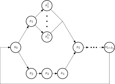
Figure 1: A discrete MDP counterexample for optimal policy under maximum entropy.

We now outline key drawbacks of merlin. It is well-understood that optimal policies under regularised Bellman operators are more stochastic than under their equivalent unregularised operators [geist19a]. While this can lead to improved exploration, the optimal policy under these operators will still be stochastic, meaning optimal deterministic policies are not learnt naturally. This leads to two difficulties: 1) a deterministic policy can be constructed by taking the action a=argmaxaπmerl(a|s)superscript𝑎subscriptargmax𝑎subscriptsuperscript𝜋merlconditional𝑎𝑠a^{*}=\operatorname*{arg\,max}_{a}\pi^{*}_{\textrm{merl}}(a|s), corresponding to the maximum a posteriori (MAP) policy, however, in continuous domains, finding the MAP policy requires optimising the Q𝑄Q-function approximator for actions, which is often a deep neural network. A common approximation is to use the mean of a variational policy instead; 2) even if we obtain a good approximation, as we show below by way of counterexample, the deterministic MAP policy is not guaranteed to be the optimal policy under Jπsuperscript𝐽𝜋J^{\pi}. Constraining the variational policies to the set of Dirac-delta distributions does not solve this problem either, since it renders the inference procedure intractable [46, 47].

Next, we demonstrate that the optimal policy under Jπsuperscript𝐽𝜋J^{\pi} cannot always be recovered from the MAP policy under Jmerlπsubscriptsuperscript𝐽𝜋merlJ^{\pi}_{\textrm{merl}}. Consider the discrete state MDP as shown in Fig. 1, with action set 𝒜={a1,a2,a11,a1k1}𝒜subscript𝑎1subscript𝑎2superscriptsubscript𝑎11superscriptsubscript𝑎1subscript𝑘1\mathcal{A}=\{a_{1},a_{2},a_{1}^{1},\cdots a_{1}^{k_{1}}\} and state set 𝒮={s0,s1,s2,s3,s4,s11s1k1,s5,s5+k2}𝒮subscript𝑠0subscript𝑠1subscript𝑠2subscript𝑠3subscript𝑠4superscriptsubscript𝑠11superscriptsubscript𝑠1subscript𝑘1subscript𝑠5subscript𝑠5subscript𝑘2\mathcal{S}=\{s_{0},s_{1},s_{2},s_{3},s_{4},s_{1}^{1}\cdots s_{1}^{k_{1}},s_{5},\cdots s_{5+{k_{2}}}\}. All state transitions are deterministic, with p(s1|s0,a1)=p(s1|s0,a2)=p(s1i|s1,a1i)=1𝑝conditionalsubscript𝑠1subscript𝑠0subscript𝑎1𝑝conditionalsubscript𝑠1subscript𝑠0subscript𝑎2𝑝conditionalsuperscriptsubscript𝑠1𝑖subscript𝑠1superscriptsubscript𝑎1𝑖1p(s_{1}|s_{0},a_{1})=p(s_{1}|s_{0},a_{2})=p(s_{1}^{i}|s_{1},a_{1}^{i})=1. All other state transitions are deterministic and independent of action taken, that is, p(sj|,sj1)=1j>2𝑝conditionalsubscript𝑠𝑗subscript𝑠𝑗11for-all𝑗2p(s_{j}|\cdot,s_{j-1})=1\ \forall\ {j>2} and p(s5|,s1i)=1𝑝conditionalsubscript𝑠5superscriptsubscript𝑠1𝑖1p(s_{5}|\cdot,s_{1}^{i})=1. The reward function is r(s0,a2)=1𝑟subscript𝑠0subscript𝑎21r(s_{0},a_{2})=1 and zero otherwise. Clearly the optimal policy under Jπsuperscript𝐽𝜋J^{\pi} has π(a2|s0)=1superscript𝜋conditionalsubscript𝑎2subscript𝑠01\pi^{*}(a_{2}|s_{0})=1. Define a maximum entropy reinforcement learning policy as πmerlsubscript𝜋merl\pi_{\textrm{merl}} with πmerl(a1|s0)=p1subscript𝜋merlconditionalsubscript𝑎1subscript𝑠0subscript𝑝1\pi_{\textrm{merl}}(a_{1}|s_{0})=p_{1}, πmerl(a2|s0)=(1p1)subscript𝜋merlconditionalsubscript𝑎2subscript𝑠01subscript𝑝1\pi_{\textrm{merl}}(a_{2}|s_{0})=(1-p_{1}) and πmerl(a1i|s1)=p1isubscript𝜋merlconditionalsuperscriptsubscript𝑎1𝑖subscript𝑠1superscriptsubscript𝑝1𝑖\pi_{\textrm{merl}}(a_{1}^{i}|s_{1})=p_{1}^{i}. For πmerlsubscript𝜋merl\pi_{\textrm{merl}} and k2>>5much-greater-thansubscript𝑘25k_{2}>>5, we can evaluate Jmerlπsubscriptsuperscript𝐽𝜋merlJ^{\pi}_{\textrm{merl}} for any scaling constant c𝑐c and discount factor γ𝛾\gamma as:

Jmerlπ=(1p1)(1clog(1p1))p1(clogp1+γci=1kp1ilogp1i).subscriptsuperscript𝐽𝜋merl1subscript𝑝11𝑐1subscript𝑝1subscript𝑝1𝑐subscript𝑝1𝛾𝑐superscriptsubscript𝑖1𝑘superscriptsubscript𝑝1𝑖superscriptsubscript𝑝1𝑖\displaystyle J^{\pi}_{\textrm{merl}}=(1-p_{1})(1-c\log(1-p_{1}))-p_{1}\left(c\log p_{1}+\gamma c\sum_{i=1}^{k}p_{1}^{i}\log p_{1}^{i}\right). (2)

We now find the optimal MERL policy. Note that p1i=1ksuperscriptsubscript𝑝1𝑖1𝑘p_{1}^{i}=\frac{1}{k} maximises the final term in Eq. 2. Substituting for p1i=1k1superscriptsubscript𝑝1𝑖1subscript𝑘1p_{1}^{i}=\frac{1}{k_{1}}, then taking derivatives of Eq. 2 with respect to p1subscript𝑝1p_{1}, and setting to zero, we find p1=πmerl(a1|s0)superscriptsubscript𝑝1superscriptsubscript𝜋merlconditionalsubscript𝑎1subscript𝑠0p_{1}^{*}=\pi_{\textrm{merl}}^{*}(a_{1}|s_{0}) as:

1clog(1p1)1𝑐1superscriptsubscript𝑝1\displaystyle 1-c\log(1-p_{1}^{*}) =γclog(k1)clogp1,absent𝛾𝑐subscript𝑘1𝑐superscriptsubscript𝑝1\displaystyle=\gamma c\log(k_{1})-c\log p_{1}^{*}, (3)
p1absentsuperscriptsubscript𝑝1\displaystyle\implies p_{1}^{*} =1k1γexp(1c)+1,absent1superscriptsubscript𝑘1𝛾1𝑐1\displaystyle=\frac{1}{{k_{1}}^{-\gamma}\exp\left(\frac{1}{c}\right)+1}, (4)

hence, for any k1γexp(1c)<1superscriptsubscript𝑘1𝛾1𝑐1{k_{1}}^{-\gamma}\exp\left(\frac{1}{c}\right)<1, we have p1>12superscriptsubscript𝑝112p_{1}^{*}>\frac{1}{2} and so πsuperscript𝜋\pi^{*} cannot be recovered from πmerlsuperscriptsubscript𝜋merl\pi_{\textrm{merl}}^{*}, even using the mode action a1=argmaxaπmerl(a|s0)subscript𝑎1subscriptargmax𝑎superscriptsubscript𝜋merlconditional𝑎subscript𝑠0a_{1}=\operatorname*{arg\,max}_{a}\pi_{\textrm{merl}}^{*}(a|s_{0}). The degree to which the MAP policy varies from the optimal unregularised policy depends on both the value of c𝑐c and k1subscript𝑘1k_{1}, the later controlling the number of states with sub-optimal reward. Our counterexample illustrates that when there are large regions of the state-space with sub-optimal reward, the temperature must be comparatively small to compensate, hence algorithms derived from merlin become very sensitive to temperature. As we discuss in Section 3.3, this problem stems from the fact that merl policies optimise for expected reward and long-term expected entropy. While initially beneficial for exploration, this can lead to sub-optimal polices being learnt in complex domains as there is often too little a priori knowledge about the MDP to make it possible to choose an appropriate value or schedule for c𝑐c.

Finally, a minor issue with merlin is that many existing models are defined for finite-horizon problems [34, 47]. While it is possible to discount and extend merlin to infinite-horizon problems, doing so is often nontrivial and can alter the objective [59, 24].

2.3 Pseudo-Likelihood Methods

A related but distinct approach is to apply Jensen’s inequality directly to the RL objective Jπsuperscript𝐽𝜋J^{\pi}. Firstly, we rewrite Eq. 1 as an expectation over τ𝜏\tau to obtain J=𝔼hp0(s)π(a|s)[Qπ(h)]=𝔼τp(τ)[R(τ)]𝐽subscript𝔼similar-tosubscript𝑝0𝑠𝜋conditional𝑎𝑠delimited-[]superscript𝑄𝜋subscript𝔼similar-to𝜏𝑝𝜏delimited-[]𝑅𝜏J=\mathbb{E}_{h\sim p_{0}(s)\pi(a|s)}\left[Q^{\pi}(h)\right]=\mathbb{E}_{\tau\sim p(\tau)}\left[R(\tau)\right], where R(τ)=t=0T1γtrt𝑅𝜏superscriptsubscript𝑡0𝑇1superscript𝛾𝑡subscript𝑟𝑡R(\tau)=\sum_{t=0}^{T-1}\gamma^{t}r_{t} and p(τ)=p0(s0)π(a0|so)t=0T1p(ht+1|ht)𝑝𝜏subscript𝑝0subscript𝑠0𝜋conditionalsubscript𝑎0subscript𝑠𝑜subscriptsuperscriptproduct𝑇1𝑡0𝑝conditionalsubscript𝑡1subscript𝑡p(\tau)=p_{0}(s_{0})\pi(a_{0}|s_{o})\prod^{T-1}_{t=0}p(h_{t+1}|h_{t}). We then treat p(R,τ)=R(τ)p(τ)𝑝𝑅𝜏𝑅𝜏𝑝𝜏p(R,\tau)=R(\tau)p(\tau) as a joint distribution, and if rewards are positive and bounded, Jensen’s inequality can be applied, enabling the derivation of an evidence lower bound (ELBO). Inference algorithms such as EM can then be employed to find a policy that optimises the pseudo-likelihood objective [12, 63, 45, 25, 43, 1]. Pseudo-likelihood methods can also be extended to a model-based setting by defining a prior over the environment’s transition dynamics. Furmston & Barber [19] demonstrate that the posterior over all possible environment models can be integrated over to obtain an optimal policy in a Bayesian setting.

Many pseudo-likelihood methods minimise KL(p𝒪pπ)KLconditionalsubscript𝑝𝒪subscript𝑝𝜋\textsc{KL}(p_{\mathcal{O}}\;\|\;p_{\pi}), where pπsubscript𝑝𝜋p_{\pi} is the policy to be learnt and p𝒪subscript𝑝𝒪p_{\mathcal{O}} is a target distribution monotonically related to reward [34]. Classical RL methods minimise KL(pπp𝒪)KLconditionalsubscript𝑝𝜋subscript𝑝𝒪\textsc{KL}(p_{\pi}\;\|\;p_{\mathcal{O}}). The latter encourages learning a mode of the target distribution, while the former encourages matching the moments of the target distribution. If the optimal policy can be represented accurately in the class of policy distributions, optimisation converges to a global optimum and the problem is fully observable, the optimal policy is the same in both cases. Otherwise, the pseudo-likelihood objective reduces the influence of large negative rewards, encouraging risk-seeking policies.

3 virel

Before describing our framework, we state some relevant assumptions.

Assumption 1 (Strictly Positive Optimal Q𝑄Q-function).

The optimal action-value function has a compact domain \mathcal{H} and is finite and strictly positive, i.e., 0<Q(h)<h0superscript𝑄for-all0<Q^{*}(h)<\infty\ \forall\ h\in\mathcal{H}.

MDPs for which rewards are lower bounded and finite, that is, R[rmin,)𝑅subscript𝑟minR\subset[r_{\mathrm{min}},\infty), satisfy the second condition of 1; we can construct a new MDP by adding rminsubscript𝑟minr_{\mathrm{min}} to the reward function, ensuring that all rewards are positive and hence the optimal Q𝑄Q-function for the reinforcement learning problem is finite and strictly positive. This does not affect the optimal solution. Now we introduce a function approximator Q^ω(h)Qπ(h)subscript^𝑄𝜔superscript𝑄𝜋\hat{Q}_{\omega}(h)\approx Q^{\pi}(h) in the bounded function space Q^ω(h)𝒬Ωsubscript^𝑄𝜔subscript𝒬Ω\hat{Q}_{\omega}(h)\in\mathcal{Q}_{\Omega}:

Definition 1 (Bounded Function Space).

Let 𝒬Ω{f:Ω×||f|<ωΩ,h}subscript𝒬Ωconditional-set𝑓formulae-sequenceΩconditional𝑓for-all𝜔Ω\mathcal{Q}_{\Omega}\coloneqq\left\{f:\Omega\times\mathcal{H}\rightarrow\mathbb{R}\ \Big{|}\ \lvert f\rvert<\infty\ \forall\ \omega\in\Omega,h\in\mathcal{H}\right\} be the space of bounded, Lipschitz continuous functions parametrised by ωΩ𝜔Ω\omega\in\Omega.

Assumption 2 (Representabilty Under Optimisation).

Our function approximator can represent the optimal Q𝑄Q-function, i.e., ωΩs.t.Q()=Q^ω()formulae-sequencesuperscript𝜔Ω𝑠𝑡superscript𝑄subscript^𝑄superscript𝜔\exists\ \omega^{*}\in\Omega\ s.t.\ Q^{*}(\cdot)=\hat{Q}_{\omega^{*}}(\cdot).

In Section F.1, we extend the work of Bhatnagar et al. [6] to continuous domains, demonstrating that 2 can be neglected if projected Bellman operators are used.

Assumption 3 (Local Smoothness of Q𝑄Q-functions ).

For ωsuperscript𝜔\omega^{*} parametrising Q()superscript𝑄Q^{*}(\cdot) in 2, Q^ω()subscript^𝑄superscript𝜔\hat{Q}_{\omega^{*}}(\cdot) has a unique maximum Q^ω(h)=suphQ^ω(h)subscript^𝑄superscript𝜔superscriptsubscriptsupremumsubscript^𝑄superscript𝜔\hat{Q}_{\omega^{*}}(h^{*})=\sup_{h}\hat{Q}_{\omega^{*}}(h). Q^ω()subscript^𝑄superscript𝜔\hat{Q}_{\omega^{*}}(\cdot) is locally 2superscript2\mathbb{C}^{2}-smooth about hsuperscripth^{*}, i.e. Δ>0s.t.Q^ω(h)2h{h|hh<Δ\exists\ \Delta>0\ s.t.\ \hat{Q}_{\omega^{*}}(h)\in\mathbb{C}^{2}\ \forall\ h\in\{h|\lVert h-h^{*}\rVert<\Delta }.

This assumption is formally required for the strict convergence of a Boltzmann to a Dirac-delta distribution and, as we discuss in Section F.4, is of more mathematical than practical concern.

3.1 Objective Specification

We now define an objective that we motivate by satisfying three desiderata: 1 In the limit of maximising our objective, a deterministic optimal policy can be recovered and the optimal Bellman equation is satisfied by our function approximator; 2 when our objective is not maximised, stochastic policies can be recovered that encourage effective exploration of the state-action space; and 3 our objective permits the application of powerful and tractable optimisation algorithms from variational inference that optimise the risk-neutral form of KL divergence, KL(pπp𝒪)KLconditionalsubscript𝑝𝜋subscript𝑝𝒪\textsc{KL}(p_{\pi}\;\|\;p_{\mathcal{O}}), introduced in Section 2.3.

Firstly, we define the residual error εωcp𝒯ωQ^ω(h)Q^ω(h)ppsubscript𝜀𝜔𝑐𝑝superscriptsubscriptdelimited-∥∥subscript𝒯𝜔subscript^𝑄𝜔subscript^𝑄𝜔𝑝𝑝\varepsilon_{\omega}\coloneqq\frac{c}{p}\lVert\mathcal{T}_{\omega}\hat{Q}_{\omega}(h)-\hat{Q}_{\omega}(h)\rVert_{p}^{p} where 𝒯ω=𝒯πωr(h)+γ𝔼hp(s|h)πω(a|s)[]\mathcal{T}_{\omega}=\mathcal{T}^{\pi_{\omega}}\bm{\cdot}\coloneqq r(h)+\gamma\mathbb{E}_{h^{\prime}\sim p(s^{\prime}|h)\pi_{\omega}(a^{\prime}|s^{\prime})}\left[\bm{\cdot}\right] is the Bellman operator for the Boltzmann policy with temperature εωsubscript𝜀𝜔\varepsilon_{\omega}:

πω(a|s)exp(Q^ω(h)εω)𝒜exp(Q^ω(h)εω)𝑑a,subscript𝜋𝜔conditional𝑎𝑠subscript^𝑄𝜔subscript𝜀𝜔subscript𝒜subscript^𝑄𝜔subscript𝜀𝜔differential-d𝑎\displaystyle\pi_{\omega}(a|s)\coloneqq\frac{\exp\left(\frac{\hat{Q}_{\omega}(h)}{\varepsilon_{\omega}}\right)}{\int_{\mathcal{A}}\exp\left(\frac{\hat{Q}_{\omega}(h)}{\varepsilon_{\omega}}\right)da}, (5)

where c>0𝑐0c>0 is an arbitrary finite constant and we assume p=2𝑝2p=2 and without loss of generality. Our main result in Theorem 2 proves that finding a ωsuperscript𝜔\omega^{*} that reduces the residual error to zero, i.e., εω=0subscript𝜀superscript𝜔0\varepsilon_{\omega^{*}}=0, is a sufficient condition for learning an optimal Q𝑄Q-function Q^ω(h)=Q(h)subscript^𝑄superscript𝜔superscript𝑄\hat{Q}_{\omega^{*}}(h)=Q^{*}(h). Additionally, the Boltzmann distribution πω(a|s)subscript𝜋𝜔conditional𝑎𝑠\pi_{\omega}(a|s) tends towards a Dirac-delta distribution πω(a|s)=δ(a=argmaxaQ^ω(a,s))subscript𝜋𝜔conditional𝑎𝑠𝛿𝑎superscriptsubscriptargmax𝑎subscript^𝑄superscript𝜔superscript𝑎𝑠\pi_{\omega}(a|s)=\delta(a=\operatorname*{arg\,max}_{a}^{\prime}\hat{Q}_{\omega^{*}}(a^{\prime},s)) whenever εω0subscript𝜀𝜔0\varepsilon_{\omega}\rightarrow 0 (see Theorem 1), which is an optimal policy. The simple objective argmin((ω))argmin(εω)argmin𝜔argminsubscript𝜀𝜔\operatorname*{arg\,min}(\mathcal{L}(\omega))\coloneqq\operatorname*{arg\,min}(\varepsilon_{\omega}) therefore satisfies 1. Moreover, when our objective is not minimised, we have εω>0subscript𝜀𝜔0\varepsilon_{\omega}>0 and from Eq. 5 we see that πω(a|s)subscript𝜋𝜔conditional𝑎𝑠\pi_{\omega}(a|s) is non-deterministic for all non-optimal ω𝜔\omega. (ω)𝜔\mathcal{L}(\omega) therefore satisfies 2 as any agent following πω(a|s)subscript𝜋𝜔conditional𝑎𝑠\pi_{\omega}(a|s) will continue exploring until the RL problem is solved. To generalise our framework, we extend 𝒯ω\mathcal{T}_{\omega}\bm{\cdot} to any operator from the set of target operators 𝒯ω𝕋\mathcal{T}_{\omega}\bm{\cdot}\in\mathbb{T}:

Definition 2 (Target Operator Set).

Define 𝕋𝕋\mathbb{T} to be the set of target operators such that an optimal Bellman operator for Q^ω(h)subscript^𝑄𝜔\hat{Q}_{\omega}(h) is recovered when the Boltzmann policy in Eq. 5 is greedy with respect to Q^ω(h)subscript^𝑄𝜔\hat{Q}_{\omega}(h), i.e., 𝕋{𝒯ω|limεω0πω(a|s)𝒯ωQ^ω(h)=𝒯Q^ω(h)}\mathbb{T}\coloneqq\{\mathcal{T}_{\omega}\bm{\cdot}|\lim_{\varepsilon_{\omega}\rightarrow 0}\pi_{\omega}(a|s)\implies\mathcal{T}_{\omega}\hat{Q}_{\omega}(h)=\mathcal{T}^{*}\hat{Q}_{\omega}(h)\}.

As an illustration, we prove in Appendix C that the Bellman operator 𝒯πω\mathcal{T}^{\pi_{\omega}}\bm{\cdot} introduced above is a member of 𝕋𝕋\mathbb{T} and can be approximated by several well-known RL targets. We also discuss how 𝒯πω\mathcal{T}^{\pi_{\omega}}\bm{\cdot} induces a constraint on ΩΩ\Omega due to its recursive definition. As we show in Section 3.2, there exists an ω𝜔\omega in the constrained domain that maximises the RL objective under these conditions, so an optimal solution is always feasible. Moreover, we provide an analysis in Section F.5 to establish that such a policy is an attractive fixed point for our algorithmic updates, even when we ignore this constraint. Off-policy operators will not constrain ΩΩ\Omega: by definition, the optimal Bellman operator 𝒯\mathcal{T}^{*}\bm{\cdot} is a member of 𝕋𝕋\mathbb{T} and does not constrain ΩΩ\Omega; similarly, we derive an off-policy operator based on a Boltzmann distribution with a diminishing temperature in Section F.2 that is a member of 𝕋𝕋\mathbb{T}. Observe that soft Bellman operators are not members of 𝕋𝕋\mathbb{T} as the optimal policy under Jmerlπsuperscriptsubscript𝐽merl𝜋J_{\text{merl}}^{\pi} is not deterministic, hence algorithms such as SAC cannot be derived from the virel framework.

One problem remains: calculating the normalisation constant to sample directly from the Boltzmann distribution in Eq. 5 is intractable for many MDPs and function approximators. As such, we look to variational inference to learn an approximate variational policy πθ(a|s)πω(a|s)subscript𝜋𝜃conditional𝑎𝑠subscript𝜋𝜔conditional𝑎𝑠\pi_{\theta}(a|s)\approx\pi_{\omega}(a|s), parametrised by θΘ𝜃Θ\theta\in\Theta with finite variance and the same support as πω(a|s)subscript𝜋𝜔conditional𝑎𝑠\pi_{\omega}(a|s). This suggests optimising a new objective that penalises πθ(a|s)subscript𝜋𝜃conditional𝑎𝑠\pi_{\theta}(a|s) when πθ(a|s)πω(a|s)subscript𝜋𝜃conditional𝑎𝑠subscript𝜋𝜔conditional𝑎𝑠\pi_{\theta}(a|s)\neq\pi_{\omega}(a|s) but still has a global maximum at εω=0subscript𝜀𝜔0\varepsilon_{\omega}=0. A tractable objective that meets these requirements is the evidence lower bound (ELBO) on the unnormalised potential of the Boltzmann distribution, defined as {ω,θ}argmaxω,θ(ω,θ)superscript𝜔superscript𝜃subscriptargmax𝜔𝜃𝜔𝜃\{\omega^{*},\theta^{*}\}\in\operatorname*{arg\,max}_{\omega,\theta}\mathcal{L}(\omega,\theta),

(ω,θ)𝜔𝜃\displaystyle\mathcal{L}(\omega,\theta) 𝔼sd(s)[𝔼aπθ(a|s)[Q^ω(h)εω]+(πθ(a|s))],absentsubscript𝔼similar-to𝑠𝑑𝑠delimited-[]subscript𝔼similar-to𝑎subscript𝜋𝜃conditional𝑎𝑠delimited-[]subscript^𝑄𝜔subscript𝜀𝜔subscript𝜋𝜃conditional𝑎𝑠\displaystyle\coloneqq\mathbb{E}_{s\sim d(s)}\left[\mathbb{E}_{a\sim\pi_{\theta}(a|s)}\left[\frac{\hat{Q}_{\omega}(h)}{\varepsilon_{\omega}}\right]+\mathscr{H}(\pi_{\theta}(a|s))\right], (6)

where qθ(h)d(s)πθ(a|s)subscript𝑞𝜃𝑑𝑠subscript𝜋𝜃conditional𝑎𝑠q_{\theta}(h)\coloneqq d(s)\pi_{\theta}(a|s) is a variational distribution, ()bold-⋅\mathscr{H}(\bm{\cdot}) denotes the differential entropy of a distribution, and d(s)𝑑𝑠d(s) is any arbitrary sampling distribution with support over 𝒮𝒮\mathcal{S}. From Eq. 6, maximising our objective with respect to ω𝜔\omega is achieved when εω0subscript𝜀𝜔0\varepsilon_{\omega}\rightarrow 0 and hence (ω,θ)𝜔𝜃\mathcal{L}(\omega,\theta) satisfies 1 and 2. As we show in Lemma 1, ()\mathscr{H}(\cdot) in Eq. 6 causes (ω,θ)𝜔𝜃\mathcal{L}(\omega,\theta)\rightarrow-\infty whenever πθ(a|s)subscript𝜋𝜃conditional𝑎𝑠\pi_{\theta}(a|s) is a Dirac-delta distribution for all εω>0subscript𝜀𝜔0\varepsilon_{\omega}>0. This means our objective heavily penalises premature convergence of our variational policy to greedy Dirac-delta policies except under optimality. We discuss a probabilistic interpretation of our framework in Appendix B, where it can be shown that πω(a|s)subscript𝜋𝜔conditional𝑎𝑠\pi_{\omega}(a|s) characterises our model’s uncertainty in the optimality of Q^ω(h)subscript^𝑄𝜔\hat{Q}_{\omega}(h).

We now motivate (ω,θ)𝜔𝜃\mathcal{L}(\omega,\theta) from an inference perspective: In Section D.1, we write (ω,θ)𝜔𝜃\mathcal{L}(\omega,\theta) in terms of the log-normalisation constant of the Boltzmann distribution and the KL divergence between the action-state normalised Boltzmann distribution, pω(h)subscript𝑝𝜔p_{\omega}(h), and the variational distribution, qθ(h)subscript𝑞𝜃q_{\theta}(h):

(ω,θ)=(ω)KL(qθ(h)pω(h))(d(s)),𝜔𝜃𝜔KLconditionalsubscript𝑞𝜃subscript𝑝𝜔𝑑𝑠\displaystyle\mathcal{L}(\omega,\theta)=\ell(\omega)-\textsc{KL}(q_{\theta}(h)\;\|\;p_{\omega}(h))-\mathscr{H}(d(s)), (7)
where(ω)logexp(Q^ω(h)εω)𝑑h,pω(h)exp(Q^ω(h)εω)exp(Q^ω(h)εω)𝑑h.formulae-sequencewhere𝜔subscriptsubscript^𝑄𝜔subscript𝜀𝜔differential-dsubscript𝑝𝜔subscript^𝑄𝜔subscript𝜀𝜔subscriptsubscript^𝑄𝜔subscript𝜀𝜔differential-d\displaystyle\mathrm{where}\quad\mathcal{\ell}(\omega)\coloneqq\log\int_{\mathcal{H}}\exp\left(\frac{\hat{Q}_{\omega}(h)}{\varepsilon_{\omega}}\right)dh,\quad p_{\omega}(h)\coloneqq\frac{\exp\left(\frac{\hat{Q}_{\omega}(h)}{\varepsilon_{\omega}}\right)}{\int_{\mathcal{H}}\exp\left(\frac{\hat{Q}_{\omega}(h)}{\varepsilon_{\omega}}\right)dh}. (8)

As the KL divergence in Eq. 7 is always positive and the final entropy term has no dependence on ω𝜔\omega or θ𝜃\theta, maximising our objective for θ𝜃\theta always reduces the KL divergence between πω(a|s)subscript𝜋𝜔conditional𝑎𝑠\pi_{\omega}(a|s) and πθ(a|s)subscript𝜋𝜃conditional𝑎𝑠\pi_{\theta}(a|s) for any εω>0subscript𝜀𝜔0\varepsilon_{\omega}>0, with πθ(a|s)=πω(a|s)subscript𝜋𝜃conditional𝑎𝑠subscript𝜋𝜔conditional𝑎𝑠\pi_{\theta}(a|s)=\pi_{\omega}(a|s) achieved under exact representability (see Theorem 3). This yields a tractable way to estimate πω(a|s)subscript𝜋𝜔conditional𝑎𝑠\pi_{\omega}(a|s) at any point during our optimisation procedure by maximising (ω,θ)𝜔𝜃\mathcal{L}(\omega,\theta) for θ𝜃\theta. From Eq. 7, we see that our objective satisfies 3, as we minimise the mode-seeking direction of KL divergence, KL(qθ(h)pω(h))KLconditionalsubscript𝑞𝜃subscript𝑝𝜔\textsc{KL}(q_{\theta}(h)\;\|\;p_{\omega}(h)), and our objective is an ELBO, which is the starting point for inference algorithms [29, 4, 17]. When the RL problem is solved and εω=0subscript𝜀𝜔0\varepsilon_{\omega}=0, our objective tends towards infinity for any variational distribution that is non-deterministic (see Lemma 1). This is of little consequence, however, as whenever εω=0subscript𝜀𝜔0\varepsilon_{\omega}=0, our approximator is the optimal value function, Q^ω(h)=Q(h)subscript^𝑄superscript𝜔superscript𝑄\hat{Q}_{\omega^{*}}(h)=Q^{*}(h) (Theorem 2), and hence, π(a|s)superscript𝜋conditional𝑎𝑠\pi^{*}(a|s) can be inferred exactly by finding maxaQ^ω(a,s)subscriptsuperscript𝑎subscript^𝑄superscript𝜔superscript𝑎𝑠\max_{a^{\prime}}\hat{Q}_{\omega^{*}}(a^{\prime},s) or by using the policy gradient θ𝔼d(s)πθ(a|s)[Q^ω(h)]subscript𝜃subscript𝔼𝑑𝑠subscript𝜋𝜃conditional𝑎𝑠delimited-[]subscript^𝑄superscript𝜔\nabla_{\theta}\mathbb{E}_{d(s)\pi_{\theta}(a|s)}\left[\hat{Q}_{\omega^{*}}(h)\right] (see Section 4.2).

3.2 Theoretical Results

We now formalise the intuition behind 1- 3. Theorem 1 establishes the emergence of a Dirac-delta distribution in the limit of εω0subscript𝜀𝜔0\varepsilon_{\omega}\rightarrow 0. To the authors’ knowledge, this is the first rigorous proof of this result. Theorem 2 shows that finding an optimal policy that maximises the RL objective in Eq. 1 reduces to finding the Boltzmann distribution associated with the parameters ωargmaxω(ω,θ)superscript𝜔subscriptargmax𝜔𝜔𝜃\omega^{*}\in\operatorname*{arg\,max}_{\omega}\mathcal{L}(\omega,\theta). The existence of such a distribution is a sufficient condition for the policy to be optimal. Theorem 3 shows that whenever εω>0subscript𝜀𝜔0\varepsilon_{\omega}>0, maximising our objective for θ𝜃\theta always reduces the KL divergence between πω(a|s)subscript𝜋𝜔conditional𝑎𝑠\pi_{\omega}(a|s) and πθ(a|s)subscript𝜋𝜃conditional𝑎𝑠\pi_{\theta}(a|s), providing a tractable method to infer the current Boltzmann policy.

Theorem 1 (Convergence of Boltzmann Distribution to Dirac Delta).

Let pε:𝒳[0,1]:subscript𝑝𝜀𝒳01p_{\varepsilon}:\mathcal{X}\rightarrow[0,1] be a Boltzmann distribution with temperature ε0𝜀subscriptabsent0\varepsilon\in\mathbb{R}_{\geq 0}, pε(x)=exp(f(x)ε)𝒳exp(f(x)ε)𝑑x,subscript𝑝𝜀𝑥𝑓𝑥𝜀subscript𝒳𝑓𝑥𝜀differential-d𝑥p_{\varepsilon}(x)=\frac{\exp\left(\frac{f(x)}{\varepsilon}\right)}{\int_{\mathcal{X}}\exp\left(\frac{f(x)}{\varepsilon}\right)dx}, where f:𝒳𝒴:𝑓𝒳𝒴f:\mathcal{X}\rightarrow\mathcal{Y} is a function that satisfies LABEL:def:locally_smooth. In the limit ε0𝜀0\varepsilon\rightarrow 0, pε(x)δ(x=supxf(x))subscript𝑝𝜀𝑥𝛿𝑥subscriptsupremumsuperscript𝑥𝑓superscript𝑥p_{\varepsilon}(x)\rightarrow\delta(x=\sup_{x^{\prime}}f(x^{\prime})).

Proof.

See Section D.2

Lemma 1 (Lower and Upper limits of (ω,θ)𝜔𝜃\mathcal{L}(\omega,\theta)).

i) For any εω>0subscript𝜀𝜔0\varepsilon_{\omega}>0 and πθ(a|s)=δ(a)subscript𝜋𝜃conditional𝑎𝑠𝛿superscript𝑎\pi_{\theta}(a|s)=\delta(a^{*}), we have (ω,θ)=𝜔𝜃\mathcal{L}(\omega,\theta)=-\infty. ii) For Q^ω(h)>0subscript^𝑄𝜔0\hat{Q}_{\omega}(h)>0 and any non-deterministic πθ(a|s)subscript𝜋𝜃conditional𝑎𝑠\pi_{\theta}(a|s), limεω0(ω,θ)=subscriptsubscript𝜀𝜔0𝜔𝜃\lim_{\varepsilon_{\omega}\rightarrow 0}\mathcal{L}(\omega,\theta)=\infty.

Proof.

See Section D.3. ∎

Theorem 2 (Optimal Boltzmann Distributions as Optimal Policies).

For ωsuperscript𝜔\omega^{*} that maximises (ω,θ)𝜔𝜃\mathcal{L}(\omega,\theta) defined in Eq. 6, the corresponding Boltzmann policy induced must be optimal, i.e., {ω,θ}argmaxω,θ(ω,θ)πω(a|s)Πsuperscript𝜔superscript𝜃subscriptargmax𝜔𝜃𝜔𝜃subscript𝜋superscript𝜔conditional𝑎𝑠superscriptΠ\{\omega^{*},\theta^{*}\}\in\operatorname*{arg\,max}_{\omega,\theta}\mathcal{L}(\omega,\theta)\implies\pi_{\omega^{*}}(a|s)\in\Pi^{*}.

Proof.

See Section D.3. ∎

Theorem 3 (Maximising the ELBO for θ𝜃\theta).

For any εω>0subscript𝜀𝜔0\varepsilon_{\omega}>0, maxθ(ω,θ)=𝔼d(s)[minθKL(πθ(a|s)πω(a|s))]\max_{\theta}\mathcal{L}(\omega,\theta)=\mathbb{E}_{d(s)}\left[\min_{\theta}\textsc{KL}(\pi_{\theta}(a|s)\;\|\;\pi_{\omega}(a|s))\right] with πω(a|s)=πθ(a|s)subscript𝜋𝜔conditional𝑎𝑠subscript𝜋𝜃conditional𝑎𝑠\pi_{\omega}(a|s)=\pi_{\theta}(a|s) under exact representability.

Proof.

See Section D.4. ∎

3.3 Comparing virel and merlin Frameworks
Refer to caption
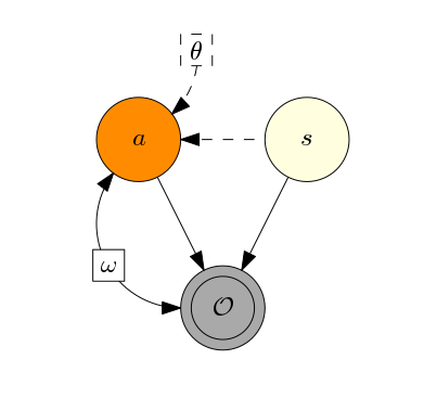
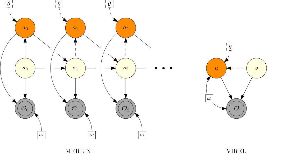
Figure 2: Graphical models for merlin and virel (variational approximations are dashed).

To compare merlin and virel, we consider the probabilistic interpretation of the two models discussed in Appendix B; introducing a binary variable 𝒪{0,1}𝒪01\mathcal{O}\in\{0,1\} defines a graphical model for our inference problem whenever εω>0subscript𝜀𝜔0\varepsilon_{\omega}>0. Comparing the graphs in Fig. 2, observe that merlin models exponential cumulative rewards over entire trajectories. By contrast, virel’s variational policy models a single step and a function approximator is used to model future expected rewards. The resulting KL divergence minimisation for merlin is therefore much more sensitive to the value of temperature, as this affects how much future entropy influences the variational policy. For virel, temperature is defined by the model, and updates to the variational policy will not be as sensitive to errors in its value or linear scaling as its influence only extends to a single interaction. We hypothesise that virel may afford advantages in higher dimensional domains where there is greater chance of encountering large regions of state-action space with sub-optimal reward; like our counterexample from Section 2, c𝑐c must be comparatively small to balance the influence of entropy in these regions to prevent merlin algorithms from learning sub-optimal policies.

Theorem 1 demonstrates that, unlike in merlin, virel naturally learns optimal deterministic policies directly from the optimisation procedure while still maintaining the benefits of stochastic policies in training. While Boltzmann policies with fixed temperatures have been proposed before [48], the adaptive temperature εωsubscript𝜀𝜔\varepsilon_{\omega} in virel’s Boltzmann policy is unique in that it ensures adaptive exploration that becomes less stochastic as Q^ω(h)Q(h)subscript^𝑄𝜔superscript𝑄\hat{Q}_{\omega}(h)\rightarrow Q^{*}(h). Like in merlin, we discuss a probabilistic interpretation of this policy as a posterior over actions conditioned on 𝒪=1𝒪1\mathcal{O}=1 in Appendix B.

4 Actor-Critic and EM

We now apply the expectation-maximisation (EM) algorithm [13, 22] to optimise our objective (ω,θ)𝜔𝜃\mathcal{L}(\omega,\theta). (See Appendix A for an exposition of this algorithm.) In keeping with RL nomenclature, we refer to Q^ω(h)subscript^𝑄𝜔\hat{Q}_{\omega}(h) as the critic and πθ(a|s)subscript𝜋𝜃conditional𝑎𝑠\pi_{\theta}(a|s) as the actor. We establish that the expectation (E-) step is equivalent to carrying out policy improvement and the maximisation (M-)step to policy evaluation. This formulation reverses the situation in most pseudo-likelihood methods, where the E-step is related to policy evaluation and the M-step is related to policy improvement, and is a direct result of optimising the forward KL divergence, KL(qθ(h)pω(h|𝒪))\textsc{KL}(q_{\theta}(h)\;\|\;p_{\omega}(h|\mathcal{O})), as opposed to the reverse KL divergence used in pseudo-likelihood methods. As discussed in Section 2.3, this mode-seeking objective prevents the algorithm from learning risk-seeking policies. We now introduce an extension to 2 that is sufficient to guarantee convergence.

Assumption 4 (Universal Variational Representability).

Every Boltzmann policy can be represented as πθ(a|s)subscript𝜋𝜃conditional𝑎𝑠\pi_{\theta}(a|s), i.e., ωΩθΘs.t.πθ(a|s)=πω(a|s)formulae-sequencefor-all𝜔Ω𝜃Θ𝑠𝑡subscript𝜋𝜃conditional𝑎𝑠subscript𝜋𝜔conditional𝑎𝑠\forall\ \omega\in\Omega\ \exists\ \theta\in\Theta\ s.t.\ \pi_{\theta}(a|s)=\pi_{\omega}(a|s).

4 is strong but, like in variational inference, our variational policy πθ(a|s)subscript𝜋𝜃conditional𝑎𝑠\pi_{\theta}(a|s) provides a useful approximation when 4 does not hold. As we discuss in Section F.1, using projected Bellman errors also ensures that our M-step always converges no matter what our current policy is.

4.1 Variational Actor-Critic

In the E-step, we keep the parameters of our critic ωksubscript𝜔𝑘\omega_{k} constant while updating the actor’s parameters by maximising the ELBO with respect to θ𝜃\theta: θk+1argmaxθ(ωk,θ)subscript𝜃𝑘1subscriptargmax𝜃subscript𝜔𝑘𝜃\theta_{k+1}\leftarrow\operatorname*{arg\,max}_{\theta}\mathcal{L}(\omega_{k},\theta). Using gradient ascent with step size αactorsubscript𝛼actor\alpha_{\textrm{actor}}, we optimise εωk(ωk,θ)subscript𝜀subscript𝜔𝑘subscript𝜔𝑘𝜃\varepsilon_{\omega_{k}}\mathcal{L}(\omega_{k},\theta) instead, which prevents ill-conditioning and does not alter the optimal solution, yielding the update (see Section E.1 for full derivation):

E-Step (Actor):

θi+1θi+αactor(εωkθ(ωk,θ))|θ=θi\theta_{i+1}\leftarrow\theta_{i}+\alpha_{\textrm{actor}}\left(\varepsilon_{\omega_{k}}\nabla_{\theta}\mathcal{L}(\omega_{k},\theta)\right)\rvert_{\theta=\theta_{i}},

εωkθ(ωk,θ)=𝔼sd(s)[𝔼aπθ(a|s)[Q^ωk(h)θlogπθ(a|s)]+εωkθ(πθ(a|s))].subscript𝜀subscript𝜔𝑘subscript𝜃subscript𝜔𝑘𝜃subscript𝔼similar-to𝑠𝑑𝑠delimited-[]subscript𝔼similar-to𝑎subscript𝜋𝜃conditional𝑎𝑠delimited-[]subscript^𝑄subscript𝜔𝑘subscript𝜃subscript𝜋𝜃conditional𝑎𝑠subscript𝜀subscript𝜔𝑘subscript𝜃subscript𝜋𝜃conditional𝑎𝑠\displaystyle\varepsilon_{\omega_{k}}\nabla_{\theta}\mathcal{L}(\omega_{k},\theta)=\mathbb{E}_{s\sim d(s)}\left[\mathbb{E}_{a\sim\pi_{\theta}(a|s)}\left[\hat{Q}_{\omega_{k}}(h)\nabla_{\theta}\log\pi_{\theta}(a|s)\right]+\varepsilon_{\omega_{k}}\nabla_{\theta}\mathscr{H}(\pi_{\theta}(a|s))\right]. (9)

In the M-step, we maximise the ELBO with respect to ω𝜔\omega while holding the parameters θk+1subscript𝜃𝑘1\theta_{k+1} constant. Hence expectations are taken with respect to the variational policy found in the E-step: ωk+1argmaxω(ω,θk+1)subscript𝜔𝑘1subscriptargmax𝜔𝜔subscript𝜃𝑘1\omega_{k+1}\leftarrow\operatorname*{arg\,max}_{\omega}\mathcal{L}(\omega,\theta_{k+1}). We use gradient ascent with step size αcritic(εωi)2subscript𝛼criticsuperscriptsubscript𝜀subscript𝜔𝑖2\alpha_{\textrm{critic}}(\varepsilon_{\omega_{i}})^{2} to optimise (ω,θk+1)𝜔subscript𝜃𝑘1\mathcal{L}(\omega,\theta_{k+1}) to prevent ill-conditioning, yielding (see Section E.2 for full derivation):

M-Step (Critic):

ωi+1ωi+αcritic(εωi)2ω(ω,θk+1)|ω=ωi,\omega_{i+1}\leftarrow\omega_{i}+\alpha_{\textrm{critic}}(\varepsilon_{\omega_{i}})^{2}\nabla_{\omega}\mathcal{L}(\omega,\theta_{k+1})\rvert_{\omega=\omega_{i}},

(εωi)2ω(ω,θk+1)=εωi𝔼d(s)πθk+1(a|s)[ωQ^ω(h)]𝔼d(s)πθk+1(a|s)[Q^ωi(h)]ωεω.superscriptsubscript𝜀subscript𝜔𝑖2subscript𝜔𝜔subscript𝜃𝑘1subscript𝜀subscript𝜔𝑖subscript𝔼𝑑𝑠subscript𝜋subscript𝜃𝑘1conditional𝑎𝑠delimited-[]subscript𝜔subscript^𝑄𝜔subscript𝔼𝑑𝑠subscript𝜋subscript𝜃𝑘1conditional𝑎𝑠delimited-[]subscript^𝑄subscript𝜔𝑖subscript𝜔subscript𝜀𝜔\displaystyle(\varepsilon_{\omega_{i}})^{2}\nabla_{\omega}\mathcal{L}(\omega,\theta_{k+1})=\varepsilon_{\omega_{i}}\mathbb{E}_{d(s)\pi_{\theta_{k+1}}(a|s)}\left[\nabla_{\omega}\hat{Q}_{\omega}(h)\right]-\mathbb{E}_{d(s)\pi_{\theta_{k+1}}(a|s)}\left[\hat{Q}_{\omega_{i}}(h)\right]\nabla_{\omega}\varepsilon_{\omega}. (10)

4.2 Discussion

From an RL perspective, the E-step corresponds to training an actor using a policy gradient method [55] with an adaptive entropy regularisation term [68, 42]. The M-step update corresponds to a policy evaluation step, as we seek to reduce the MSBE in the second term of Eq. 10. We derive ωεωsubscript𝜔subscript𝜀𝜔\nabla_{\omega}\varepsilon_{\omega} exactly in Section E.3. Note that this term depends on (𝒯ωQ^ω(h)Q^ω(h))ω𝒯ωQ^ω(h)subscript𝒯𝜔subscript^𝑄𝜔subscript^𝑄𝜔subscript𝜔subscript𝒯𝜔subscript^𝑄𝜔(\mathcal{T}_{\omega}\hat{Q}_{\omega}(h)-\hat{Q}_{\omega}(h))\nabla_{\omega}\mathcal{T}_{\omega}\hat{Q}_{\omega}(h), which typically requires evaluating two independent expectations. For convergence guarantees, techniques such as residual gradients [2] or GTD2/TDC [6] need to be employed to obtain an unbiased estimate of this term. If guaranteed convergence is not a priority, dropping gradient terms allows us to use direct methods [54], which are often simpler to implement. We discuss these methods further in Section F.3 and provide an analysis in Section F.5 demonstrating that the corresponding updates act as a variational approximation to Q𝑄Q-learning [67, 41]. A key component of our algorithm is the behaviour when εω=0subscript𝜀superscript𝜔0\varepsilon_{\omega^{*}}=0; under this condition, there is no M-step update (both εωk=0subscript𝜀subscript𝜔𝑘0\varepsilon_{\omega_{k}}=0 and ωεω=0subscript𝜔subscript𝜀𝜔0\nabla_{\omega}\varepsilon_{\omega}=0) and Qω(h)=Q(h)subscript𝑄superscript𝜔superscript𝑄Q_{\omega^{*}}(h)=Q^{*}(h) (see Theorem 2), so our E-step reduces exactly to a policy gradient step, θk+1θk+αactor𝔼hd(s)πθ(a|s)[Q(h)θlogπθ(a|s)]subscript𝜃𝑘1subscript𝜃𝑘subscript𝛼actorsubscript𝔼similar-to𝑑𝑠subscript𝜋𝜃conditional𝑎𝑠delimited-[]superscript𝑄subscript𝜃subscript𝜋𝜃conditional𝑎𝑠\theta_{k+1}\leftarrow\theta_{k}+\alpha_{\textrm{actor}}\mathbb{E}_{h\sim d(s)\pi_{\theta}(a|s)}\left[Q^{*}(h)\nabla_{\theta}\log\pi_{\theta}(a|s)\right], recovering the optimal policy in the limit of convergence, that is, πθ(a|s)π(a|s)subscript𝜋𝜃conditional𝑎𝑠superscript𝜋conditional𝑎𝑠\pi_{\theta}(a|s)\rightarrow\pi^{*}(a|s).

From an inference perspective, the E-step improves the parameters of our variational distribution to reduce the gap between the current Boltzmann posterior and the variational policy, KL(πθ(a|s))πωk(a|s))\textsc{KL}(\pi_{\theta}(a|s))\;\|\;\pi_{\omega_{k}}(a|s)) (see Theorem 3). This interpretation makes precise the intuition that how much we can improve our policy is determined by how similar Q^ωk(h)subscript^𝑄subscript𝜔𝑘\hat{Q}_{\omega_{k}}(h) is to Q(h)superscript𝑄Q^{*}(h), limiting policy improvement to the complete E-step: πθk+1(a|s)=πωk(a|s)subscript𝜋subscript𝜃𝑘1conditional𝑎𝑠subscript𝜋subscript𝜔𝑘conditional𝑎𝑠\pi_{\theta_{k+1}}(a|s)=\pi_{\omega_{k}}(a|s). We see that the common greedy policy improvement step, πθk+1(a|s)=δ(aargmaxa(Q^ωk(a,s)))subscript𝜋subscript𝜃𝑘1conditional𝑎𝑠𝛿𝑎subscriptargmaxsuperscript𝑎subscript^𝑄subscript𝜔𝑘superscript𝑎𝑠\pi_{\theta_{k+1}}(a|s)=\delta(a\in\operatorname*{arg\,max}_{a^{\prime}}(\hat{Q}_{\omega_{k}}(a^{\prime},s))) acts as an approximation to the Boltzmann form in Eq. 5, replacing the softmax with a hard maximum.

If 4 holds and any constraint induced by 𝒯ω\mathcal{T}_{\omega}\bm{\cdot} does not prevent convergence to a complete E-step, the EM algorithm alternates between two convex optimisation schemes, and is guaranteed to converge to at least a local optimum of (ω,θ)𝜔𝜃\mathcal{L}(\omega,\theta) [70]. In reality, we cannot carry out complete E- and M-steps for complex domains, and our variational distributions are unlikely to satisfy 4. Under these conditions, we can resort to the empirically successful variational EM algorithm [29], carrying out partial E- and M-steps instead, which we discuss further in Section F.3.

4.3 Advanced Actor-Critic Methods

A family of actor-critic algorithms follows naturally from our framework: 1) we can use powerful inference techniques such as control variates [21] or variance-reducing baselines by subtracting any function that does not depend on the action [49], e.g., V(s)𝑉𝑠V(s), from the action-value function, as this does not change our objective, 2) we can manipulate Eq. 9 to obtain variance-reducing gradient estimators such as EPG [11], FPG [15], and SVG0 [27], and 3) we can take advantage of d(s)𝑑𝑠d(s) being any general decorrelated distribution by using replay buffers [41] or empirically successful asynchronous methods that combine several agents’ individual gradient updates at once [42]. As we discuss in Section E.4, the manipulation required to derive the estimators in 2) is not strictly justified in the classic policy gradient theorem [55] and MERL formulation [24].

MPO is a state-of-the-art EM algorithm derived from the pseudo-likelihood objective [1]. In its derivation, policy evaluation does not naturally arise from either of its EM steps and must be carried out separately. In addition, its E step is approximated, giving rise to the one step KL regularised update. As we demonstrate in Appendix G, under the probabilistic interpretation of our model, including a prior of the form pϕ(h)=𝒰(s)πϕ(a|s)subscript𝑝italic-ϕ𝒰𝑠subscript𝜋italic-ϕconditional𝑎𝑠p_{\phi}(h)=\mathcal{U}(s)\pi_{\phi}(a|s) in our ELBO and specifying a hyper-prior p(ω)𝑝𝜔p(\omega), the MPO objective with an adaptive regularisation constant can be recovered from virel:

mpo(ω,θ,ϕ)=𝔼sd(s)[𝔼aπθ(a|s)[Q^ω(h)εω]KL(πθ(a|s)πϕ(a|s))]+logp(ω).\displaystyle\mathcal{L}^{\textsc{mpo}}(\omega,\theta,\phi)=\mathbb{E}_{s\sim d(s)}\left[\mathbb{E}_{a\sim\pi_{\theta}(a|s)}\left[\frac{\hat{Q}_{\omega}(h)}{\varepsilon_{\omega}}\right]-\textsc{KL}(\pi_{\theta}(a|s)\;\|\;\pi_{\phi}(a|s))\right]+\log p(\omega). (11)

We also show in Appendix G that applying the (variational) EM algorithm from Section 4 yields the MPO updates with the missing policy evaluation step and without approximation in the E-step.

5 Experiments

We evaluate our EM algorithm using the direct method approximation outlined in Section F.3 with 𝒯ωsubscript𝒯𝜔\mathcal{T}_{\omega}, ignoring constraints on ΩΩ\Omega. The aim of our evaluation is threefold: Firstly, as explained in Section 3.1, algorithms using soft value functions cannot be recovered from virel. We therefore demonstrate that using hard value functions does not affect performance. Secondly, we provide evidence for our hypothesis stated in Section 3.3 that using soft value functions may harm performance in higher dimensional tasks. Thirdly, we show that even under all practical approximations discussed, the algorithm derived in Section 4 still outperforms advanced actor-critic methods.

We compare our methods to the state-of-the-art SAC111We use implementations provided by the authors https://github.com/haarnoja/sac for v1 and https://github.com/vitchyr/rlkit for v2. and DDPG [37] algorithms on MuJoCo tasks in OpenAI gym [9] and in rllab [14]. We use SAC as a baseline because Haarnoja et al. [24] show that it outperforms PPO [51], Soft Q𝑄Q-Learning [23], and TD3 [18]. We compare to DDPG [37] because, like our methods, it can learn deterministic optimal policies. We consider two variants: In the first one, called virel, we keep the scale of the entropy term in the gradient update for the variational policy constant α𝛼\alpha; in the second, called beta, we use an estimate ε^ωsubscript^𝜀𝜔\hat{\varepsilon}_{\omega} of εωsubscript𝜀𝜔\varepsilon_{\omega} to scale the corresponding term in Eq. 132. We compute ε^ωsubscript^𝜀𝜔\hat{\varepsilon}_{\omega} using a buffer to draw a fixed number of samples Nεsubscript𝑁𝜀N_{\varepsilon} for the estimate.

Refer to caption
Refer to caption
Refer to caption
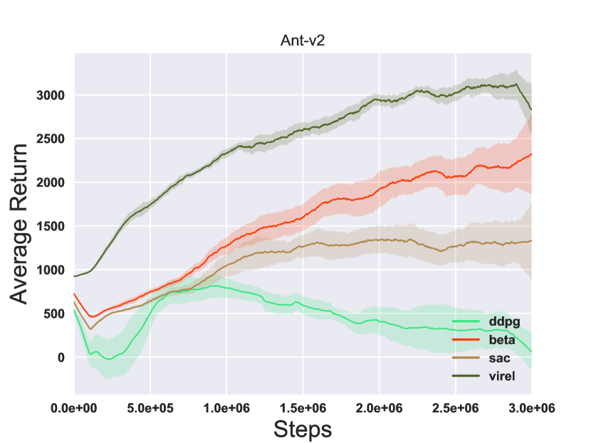
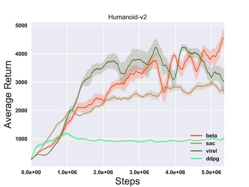
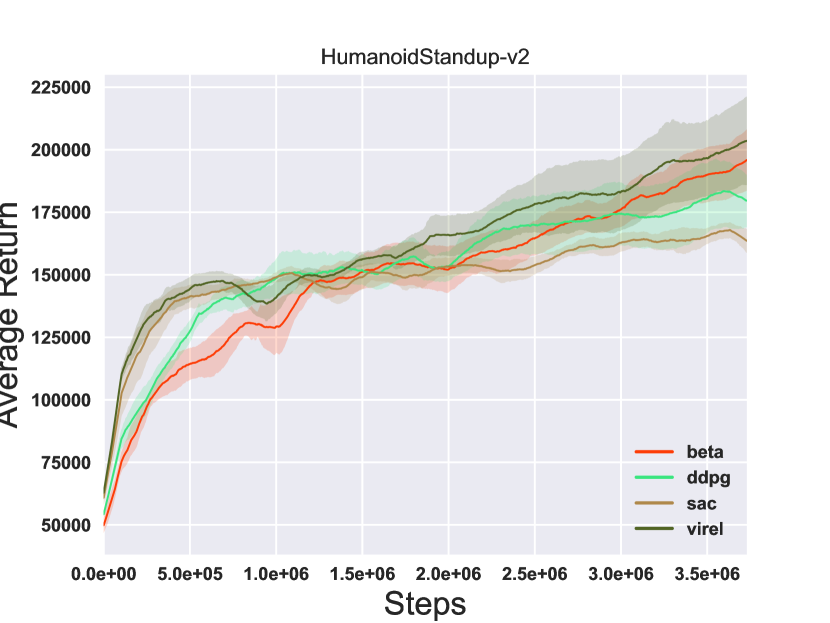
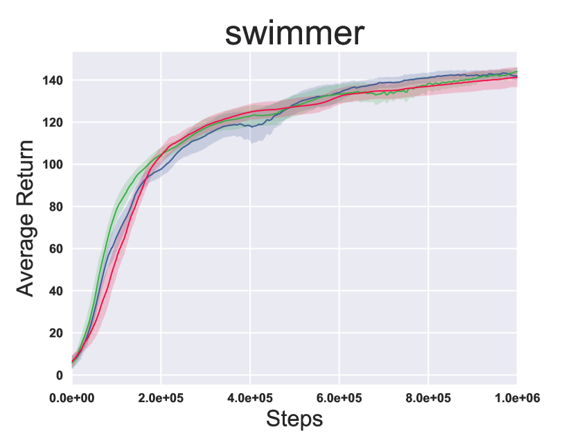
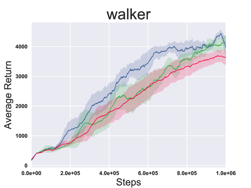
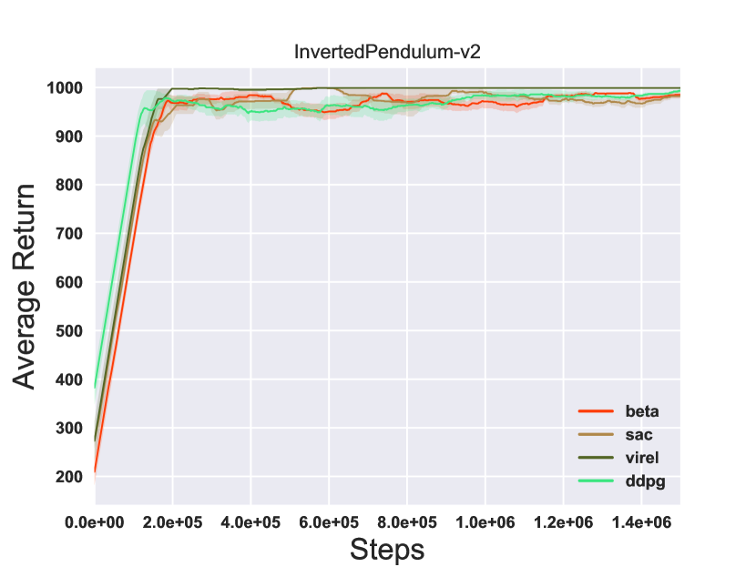
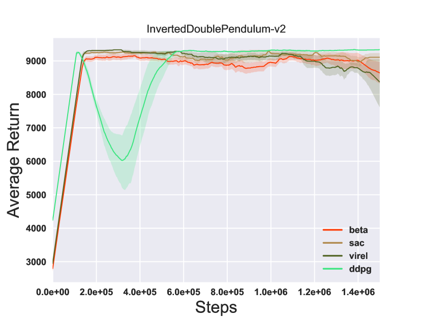
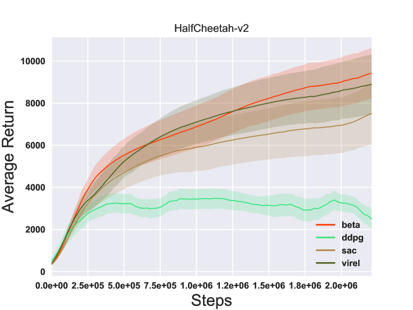
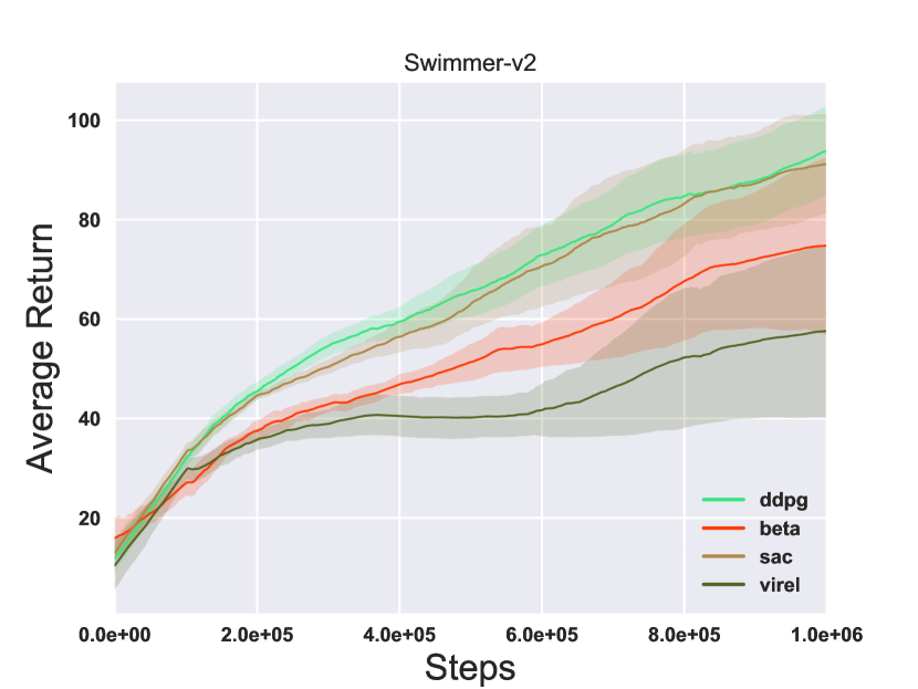
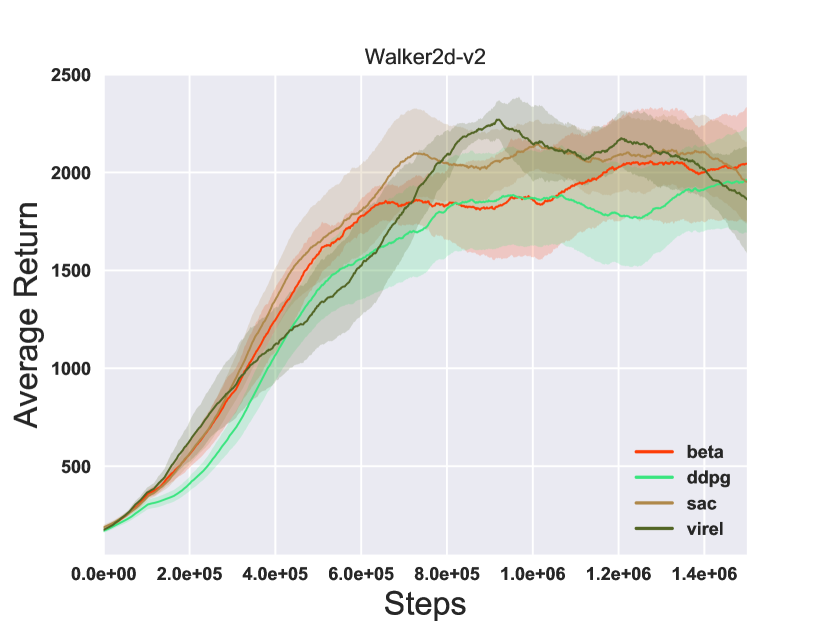
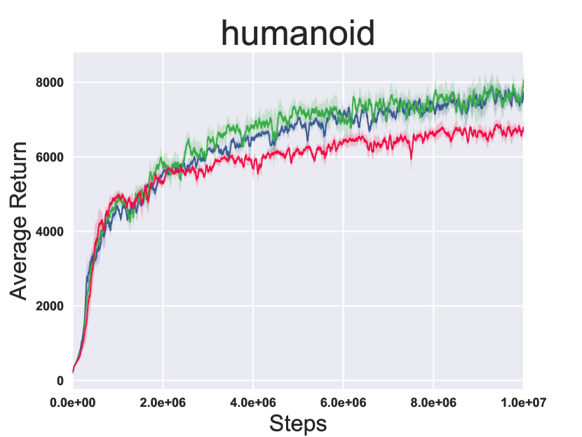
Figure 3: Training curves on continuous control benchmarks gym-Mujoco-v2 : High-dimensional domains.

To adjust for the relative magnitude of the first term in Eq. 132 with that of εωsubscript𝜀𝜔\varepsilon_{\omega} scaling the second term, we also multiply the estimate ε^ωsubscript^𝜀𝜔\hat{\varepsilon}_{\omega} by a scalar λ1γravg𝜆1𝛾subscript𝑟𝑎𝑣𝑔\lambda\approx\frac{1-\gamma}{r_{avg}}, where ravgsubscript𝑟𝑎𝑣𝑔r_{avg} is the average reward observed; λ1superscript𝜆1\lambda^{-1} roughly captures the order of magnitude of the first term and allows ε^ωsubscript^𝜀𝜔\hat{\varepsilon}_{\omega} to balance policy changes between exploration and exploitation. We found performance is poor and unstable without λ𝜆\lambda. To reduce variance, all algorithms use a value function network V(ϕ)𝑉italic-ϕV(\phi) as a baseline and a Gaussian policy, which enables the use of the reparametrisation trick. Pseudocode can be found in Appendix H. All experiments use 5 random initialisations and parameter values are given in Section I.1.

Fig. 3 gives the training curves for the various algorithms on high-dimensional tasks for on gym-mujoco-v2. In particular, in Humanoid-v2 (action space dimensionality: 17, state space dimensionality: 376) and Ant-v2 (action space dimensionality: 8, state space dimensionality: 111), DDPG fails to learn any reasonable policy. We believe that this is because the Ornstein-Uhlenbeck noise that DDPG uses for exploration is insufficiently adaptive in high dimensions. While SAC performs better, virel and beta still significantly outperform it. As hypothesised in Section 3.3, we believe that this performance advantage arises because the gap between optimal unregularised policies and optimal variational policies learnt under merlin is sensitive to temperature c𝑐c. This effect is exacerbated in high dimensions where there may be large regions of the state-action space with sub-optimal reward. All algorithms learn optimal policies in simple domains, the training curves for which can be found in Fig. 8 in Section I.3. Thus, as the state-action dimensionality increases, algorithms derived from virel outperform SAC and DDPG.

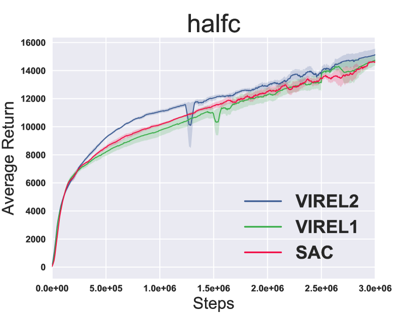
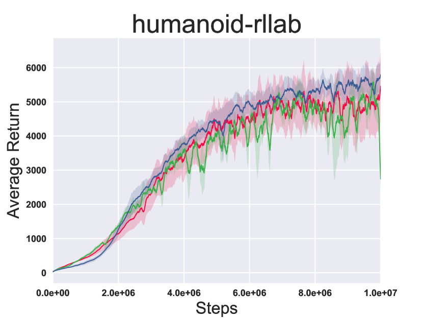
Fujimoto et al. [18] and van Hasselt et al. [66] note that using the minimum of two randomly initialised action-value functions helps mitigate the positive bias introduced by function approximation in policy gradient methods. Therefore, a variant of SAC uses two soft critics. We compare this variant of SAC to two variants of virel: virel1, which uses two hard Q𝑄Q-functions and virel2, which uses one hard and one soft Q𝑄Q-function. We scale the rewards so that the means of the Q𝑄Q-function estimates in virel2 are approximately aligned. Fig. 4 shows the training curves on three gym-Mujoco-v1 domains, with additional plots shown in Fig. 7 in Section I.2. Again, the results demonstrate that virel1 and virel2 perform on par with SAC in simple domains like Half-Cheetah and outperform it in challenging high-dimensional domains like humanoid-gym and -rllab (17 and 21 dimensional action spaces, 376 dimensional state space).
Refer to caption
Refer to caption
Refer to caption
Figure 4: Training curves on continuous control benchmarks gym-Mujoco-v1.

6 Conclusion and Future Work

This paper presented virel, a novel framework that recasts the reinforcement learning problem as an inference problem using function approximators. We provided strong theoretical justifications for this framework and compared two simple actor-critic algorithms that arise naturally from applying variational EM on the objective. Extensive empirical evaluation shows that our algorithms perform on par with current state-of-the-art methods on simple domains and substantially outperform them on challenging high dimensional domains. As immediate future work, our focus is to find better estimates of εωsubscript𝜀𝜔\varepsilon_{\omega} to provide a principled method for uncertainty based exploration; we expect it to help attain sample efficiency in conjunction with various methods like [38, 39]. Another avenue of research would extend our framework to multi-agent settings, in which it can be used to tackle the sub-optimality induced by representational constraints used in MARL algorithms [40].

7 Acknowledgements

This project has received funding from the European Research Council (ERC) under the European Unions Horizon 2020 research and innovation programme (grant agreement number 637713). The experiments were made possible by a generous equipment grant from NVIDIA. Matthew Fellows is funded by the EPSRC. Anuj Mahajan is funded by Google DeepMind and the Drapers Scholarship. Tim G. J. Rudner is funded by the Rhodes Trust and the EPSRC. We would like to thank Yarin Gal and Piotr Miloś for helpful comments.

References

  • Abdolmaleki et al. [2018] Abdolmaleki, A., Springenberg, J. T., Tassa, Y., Munos, R., Heess, N., and Riedmiller, M. Maximum a posteriori policy optimisation. In International Conference on Learning Representations, 2018. URL https://openreview.net/forum?id=S1ANxQW0b.
  • Baird [1995] Baird, L. Residual algorithms: Reinforcement learning with function approximation. Machine Learning-International Workshop Then Conference-, (July):30–37, 1995. ISSN 00043702. doi: 10.1.1.48.3256.
  • Bass [2013] Bass, R. Real Analysis for Graduate Students. Createspace Ind Pub, 2013. ISBN 9781481869140. URL https://books.google.co.uk/books?id=s6mVlgEACAAJ.
  • Beal [2003] Beal, M. J. Variational algorithms for approximate Bayesian inference. PhD thesis, 2003.
  • Bertsekas [1996] Bertsekas, D. Constrained Optimization and Lagrange Multiplier Methods. Athena scientific series in optimization and neural computation. Athena Scientific, 1996. ISBN 9781886529045. URL http://web.mit.edu/dimitrib/www/Constrained-Opt.pdf.
  • Bhatnagar et al. [2009] Bhatnagar, S., Precup, D., Silver, D., Sutton, R. S., Maei, H. R., and Szepesvári, C. Convergent temporal-difference learning with arbitrary smooth function approximation. In Bengio, Y., Schuurmans, D., Lafferty, J. D., Williams, C. K. I., and Culotta, A. (eds.), Advances in Neural Information Processing Systems 22, pp.  1204–1212. Curran Associates, Inc., 2009.
  • Bishop [2006] Bishop, C. M. Pattern Recognition and Machine Learning (Information Science and Statistics). Springer-Verlag New York, Inc., Secaucus, NJ, USA, 2006. ISBN 0387310738.
  • Blei et al. [2017] Blei, D. M., Kucukelbir, A., and McAuliffe, J. D. Variational Inference: A Review for Statisticians, 2017. ISSN 1537274X.
  • Brockman et al. [2016] Brockman, G., Cheung, V., Pettersson, L., Schneider, J., Schulman, J., Tang, J., and Zaremba, W. Openai gym. CoRR, abs/1606.01540, 2016. URL http://arxiv.org/abs/1606.01540.
  • Ciosek & Whiteson [2018a] Ciosek, K. and Whiteson, S. Expected Policy Gradients. The Thirty-Second AAAI Conference on Artificial Intelligence (AAAI-18), 2018a.
  • Ciosek & Whiteson [2018b] Ciosek, K. and Whiteson, S. Expected policy gradients for reinforcement learning. journal submission, arXiv preprint arXiv:1801.03326, 2018b.
  • Dayan & Hinton [1997] Dayan, P. and Hinton, G. E. Using expectation-maximization for reinforcement learning. Neural Computation, 9(2):271–278, 1997. doi: 10.1162/neco.1997.9.2.271. URL https://doi.org/10.1162/neco.1997.9.2.271.
  • Dempster et al. [1977] Dempster, A. P., Laird, N. M., and Rubin, D. B. Maximum likelihood from incomplete data via the em algorithm. Journal of the Royal Statistical Society, Series B, 39(1):1–38, 1977.
  • Duan et al. [2016] Duan, Y., Chen, X., Houthooft, R., Schulman, J., and Abbeel, P. Benchmarking deep reinforcement learning for continuous control. In International Conference on Machine Learning, pp. 1329–1338, 2016.
  • Fellows et al. [2018] Fellows, M., Ciosek, K., and Whiteson, S. Fourier policy gradients. In Dy, J. and Krause, A. (eds.), Proceedings of the 35th International Conference on Machine Learning, volume 80 of Proceedings of Machine Learning Research, pp.  1486–1495, Stockholmsmässan, Stockholm Sweden, 10–15 Jul 2018. PMLR. URL http://proceedings.mlr.press/v80/fellows18a.html.
  • Foerster et al. [2018] Foerster, J., Farquhar, G., Al-Shedivat, M., Rocktäschel, T., Xing, E., and Whiteson, S. DiCE: The infinitely differentiable Monte Carlo estimator. In Dy, J. and Krause, A. (eds.), Proceedings of the 35th International Conference on Machine Learning, volume 80 of Proceedings of Machine Learning Research, pp.  1529–1538, Stockholmsmässan, Stockholm Sweden, 10–15 Jul 2018. PMLR. URL http://proceedings.mlr.press/v80/foerster18a.html.
  • Fox & Roberts [2010] Fox, C. W. and Roberts, S. J. A tutorial on variational Bayesian inference. Artificial Intelligence Review, pp.  1–11, 2010. ISSN 0269-2821. doi: 10.1007/s10462-011-9236-8. URL papers2://publication/uuid/1B6D2DDA-67F6-4EEE-9720-2907FFB14789.
  • Fujimoto et al. [2018] Fujimoto, S., van Hoof, H., and Meger, D. Addressing function approximation error in actor-critic methods. In Dy, J. and Krause, A. (eds.), Proceedings of the 35th International Conference on Machine Learning, volume 80 of Proceedings of Machine Learning Research, pp.  1587–1596, Stockholmsmässan, Stockholm Sweden, 10–15 Jul 2018. PMLR. URL http://proceedings.mlr.press/v80/fujimoto18a.html.
  • Furmston & Barber [2010] Furmston, T. and Barber, D. Variational Methods For Reinforcement Learning. In AISTATS, pp.  241–248, 2010. ISSN 15324435.
  • Goyal et al. [2018] Goyal, A., Brakel, P., Fedus, W., Lillicrap, T. P., Levine, S., Larochelle, H., and Bengio, Y. Recall traces: Backtracking models for efficient reinforcement learning. CoRR, abs/1804.00379, 2018. URL http://arxiv.org/abs/1804.00379.
  • Gu et al. [2016] Gu, S., Lillicrap, T., Ghahramani, Z., Turner, R. E., and Levine, S. Q-Prop: Sample-Efficient Policy Gradient with An Off-Policy Critic. pp.  1–13, 2016. URL http://arxiv.org/abs/1611.02247.
  • Gunawardana & Byrne [2005] Gunawardana, A. and Byrne, W. Convergence theorems for generalized alternating minimization procedures. J. Mach. Learn. Res., 6:2049–2073, December 2005. ISSN 1532-4435. URL http://dl.acm.org/citation.cfm?id=1046920.1194913.
  • Haarnoja et al. [2017] Haarnoja, T., Tang, H., Abbeel, P., and Levine, S. Reinforcement learning with deep energy-based policies. In Precup, D. and Teh, Y. W. (eds.), Proceedings of the 34th International Conference on Machine Learning, volume 70 of Proceedings of Machine Learning Research, pp.  1352–1361, International Convention Centre, Sydney, Australia, 06–11 Aug 2017. PMLR. URL http://proceedings.mlr.press/v70/haarnoja17a.html.
  • Haarnoja et al. [2018] Haarnoja, T., Zhou, A., Abbeel, P., and Levine, S. Soft actor-critic: Off-policy maximum entropy deep reinforcement learning with a stochastic actor. In Dy, J. and Krause, A. (eds.), Proceedings of the 35th International Conference on Machine Learning, volume 80 of Proceedings of Machine Learning Research, pp.  1861–1870, Stockholmsmässan, Stockholm Sweden, 10–15 Jul 2018. PMLR. URL http://proceedings.mlr.press/v80/haarnoja18b.html.
  • Hachiya et al. [2009] Hachiya, H., Peters, J., and Sugiyama, M. Efficient sample reuse in em-based policy search. In Buntine, W., Grobelnik, M., Mladenić, D., and Shawe-Taylor, J. (eds.), Machine Learning and Knowledge Discovery in Databases, pp. 469–484, Berlin, Heidelberg, 2009. Springer Berlin Heidelberg. ISBN 978-3-642-04180-8.
  • Heess et al. [2013] Heess, N., Silver, D., and Teh, Y. W. Actor-critic reinforcement learning with energy-based policies. In Deisenroth, M. P., Szepesvári, C., and Peters, J. (eds.), Proceedings of the Tenth European Workshop on Reinforcement Learning, volume 24 of Proceedings of Machine Learning Research, pp.  45–58, Edinburgh, Scotland, 30 Jun–01 Jul 2013. PMLR. URL http://proceedings.mlr.press/v24/heess12a.html.
  • Heess et al. [2015a] Heess, N., Wayne, G., Silver, D., Lillicrap, T., Erez, T., and Tassa, Y. Learning continuous control policies by stochastic value gradients. In Cortes, C., Lawrence, N. D., Lee, D. D., Sugiyama, M., and Garnett, R. (eds.), Advances in Neural Information Processing Systems 28, pp.  2944–2952. Curran Associates, Inc., 2015a.
  • Heess et al. [2015b] Heess, N., Wayne, G., Silver, D., Lillicrap, T., Tassa, Y., and Erez, T. Learning Continuous Control Policies by Stochastic Value Gradients. pp.  1–13, 2015b. ISSN 10495258. URL http://arxiv.org/abs/1510.09142.
  • Jordan [1999] Jordan, M. I. (ed.). Learning in Graphical Models. MIT Press, Cambridge, MA, USA, 1999. ISBN 0-262-60032-3.
  • Kelly [2008] Kelly, J. Generalized Functions, chapter 4, pp.  111–124. John Wiley & Sons, Ltd, 2008. ISBN 9783527618897. doi: 10.1002/9783527618897.ch4. URL https://onlinelibrary.wiley.com/doi/abs/10.1002/9783527618897.ch4.
  • Kingma & Welling [2014] Kingma, D. P. and Welling, M. Auto-Encoding Variational Bayes PPT. Proceedings of the 2nd International Conference on Learning Representations (ICLR), 2014. ISSN 1312.6114v10. URL http://arxiv.org/abs/1312.6114.
  • Koller & Parr [2000] Koller, D. and Parr, R. Policy iteration for factored mdps. In Proceedings of the Sixteenth Conference on Uncertainty in Artificial Intelligence, UAI’00, pp.  326–334, San Francisco, CA, USA, 2000. Morgan Kaufmann Publishers Inc. ISBN 1-55860-709-9. URL http://dl.acm.org/citation.cfm?id=2073946.2073985.
  • Levine [2014] Levine, S. Motor Skill Learning with Trajectory Methods. PhD thesis, 2014. URL https://people.eecs.berkeley.edu/{~}svlevine/papers/thesis.pdf.
  • Levine [2018] Levine, S. Reinforcement Learning and Control as Probabilistic Inference: Tutorial and Review. 2018. URL https://arxiv.org/pdf/1805.00909.pdf.
  • Levine & Koltun [2013] Levine, S. and Koltun, V. Variational policy search via trajectory optimization. In Burges, C. J. C., Bottou, L., Welling, M., Ghahramani, Z., and Weinberger, K. Q. (eds.), Advances in Neural Information Processing Systems 26, pp.  207–215. Curran Associates, Inc., 2013.
  • Liberzon [2011] Liberzon, D. Calculus of Variations and Optimal Control Theory: A Concise Introduction. Princeton University Press, Princeton, NJ, USA, 2011. ISBN 0691151873, 9780691151878.
  • Lillicrap et al. [2015] Lillicrap, T. P., Hunt, J. J., Pritzel, A., Heess, N., Erez, T., Tassa, Y., Silver, D., and Wierstra, D. Continuous control with deep reinforcement learning. arXiv preprint arXiv:1509.02971, 2015.
  • Mahajan & Tulabandhula [2017a] Mahajan, A. and Tulabandhula, T. Symmetry learning for function approximation in reinforcement learning. arXiv preprint arXiv:1706.02999, 2017a.
  • Mahajan & Tulabandhula [2017b] Mahajan, A. and Tulabandhula, T. Symmetry detection and exploitation for function approximation in deep rl. In Proceedings of the 16th Conference on Autonomous Agents and MultiAgent Systems, pp.  1619–1621. International Foundation for Autonomous Agents and Multiagent Systems, 2017b.
  • Mahajan et al. [2019] Mahajan, A., Rashid, T., Samvelyan, M., and Whiteson, S. Maven: Multi-agent variational exploration, 2019. URL https://arxiv.org/abs/1910.07483.
  • Mnih et al. [2015] Mnih, V., Kavukcuoglu, K., Silver, D., Rusu, A. A., Veness, J., Bellemare, M. G., Graves, A., Riedmiller, M., Fidjeland, A. K., Ostrovski, G., Petersen, S., Beattie, C., Sadik, A., Antonoglou, I., King, H., Kumaran, D., Wierstra, D., Legg, S., and Hassabis, D. Human-level control through deep reinforcement learning. Nature, 518(7540):529–533, 2015. ISSN 14764687. doi: 10.1038/nature14236.
  • Mnih et al. [2016] Mnih, V., Badia, A. P., Mirza, M., Graves, A., Lillicrap, T., Harley, T., Silver, D., and Kavukcuoglu, K. Asynchronous methods for deep reinforcement learning. In Balcan, M. F. and Weinberger, K. Q. (eds.), Proceedings of The 33rd International Conference on Machine Learning, volume 48 of Proceedings of Machine Learning Research, pp.  1928–1937, New York, New York, USA, 20–22 Jun 2016. PMLR. URL http://proceedings.mlr.press/v48/mniha16.html.
  • Neumann [2011] Neumann, G. Variational inference for policy search in changing situations. In Proceedings of the 28th International Conference on International Conference on Machine Learning, ICML’11, pp.  817–824, USA, 2011. Omnipress. ISBN 978-1-4503-0619-5. URL http://dl.acm.org/citation.cfm?id=3104482.3104585.
  • Pearlmutter [1994] Pearlmutter, B. A. Fast exact multiplication by the hessian. Neural Computation, 6:147–160, 1994.
  • Peters & Schaal [2007] Peters, J. and Schaal, S. Reinforcement learning by reward-weighted regression for operational space control. In Proceedings of the 24th International Conference on Machine Learning, ICML ’07, pp.  745–750, New York, NY, USA, 2007. ACM. ISBN 978-1-59593-793-3. doi: 10.1145/1273496.1273590. URL http://doi.acm.org/10.1145/1273496.1273590.
  • Rawlik et al. [2010] Rawlik, K., Toussaint, M., and Vijayakumar, S. Approximate inference and stochastic optimal control. CoRR, abs/1009.3958, 2010. URL http://arxiv.org/abs/1009.3958.
  • Rawlik et al. [2012] Rawlik, K., Toussaint, M., and Vijayakumar, S. On stochastic optimal control and reinforcement learning by approximate inference. In Robotics: Science and Systems, 2012.
  • Sallans & Hinton [2004] Sallans, B. and Hinton, G. E. Reinforcement learning with factored states and actions. J. Mach. Learn. Res., 5:1063–1088, dec 2004. ISSN 1532-4435. URL http://dl.acm.org/citation.cfm?id=1005332.1016794.
  • Schulman et al. [2015a] Schulman, J., Heess, N., Weber, T., and Abbeel, P. Gradient estimation using stochastic computation graphs. In Cortes, C., Lawrence, N. D., Lee, D. D., Sugiyama, M., and Garnett, R. (eds.), Advances in Neural Information Processing Systems 28, pp.  3528–3536. Curran Associates, Inc., 2015a.
  • Schulman et al. [2015b] Schulman, J., Levine, S., Abbeel, P., Jordan, M., and Moritz, P. Trust region policy optimization. 37:1889–1897, 07–09 Jul 2015b. URL http://proceedings.mlr.press/v37/schulman15.html.
  • Schulman et al. [2017] Schulman, J., Wolski, F., Dhariwal, P., Radford, A., and Klimov, O. Proximal policy optimization algorithms. CoRR, abs/1707.06347, 2017.
  • Silver et al. [2014] Silver, D., Lever, G., Heess, N., Degris, T., Wierstra, D., and Riedmiller, M. Deterministic Policy Gradient Algorithms. Proceedings of the 31st International Conference on Machine Learning (ICML-14), pp.  387–395, 2014. ISSN 1938-7228.
  • Sutton & Barto [1998] Sutton, R. S. and Barto, A. G. Sutton & Barto Book: Reinforcement Learning: An Introduction. MIT Press, Cambridge, MA, A Bradford Book, 1998. ISSN 10459227. doi: 10.1109/TNN.1998.712192.
  • Sutton & Barto [2017] Sutton, R. S. and Barto, A. G. Introduction to Reinforcement Learning. MIT Press, Cambridge, MA, USA, 2nd edition, 2017. ISBN 0262193981.
  • Sutton et al. [1999] Sutton, R. S., Mcallester, D., Singh, S., and Mansour, Y. Policy Gradient Methods for Reinforcement Learning with Function Approximation. Advances in Neural Information Processing Systems 12, pp. 1057–1063, 1999. ISSN 0047-2875. doi: 10.1.1.37.9714.
  • Sutton et al. [2009a] Sutton, R. S., Maei, H. R., Precup, D., Bhatnagar, S., Silver, D., Szepesvári, C., and Wiewiora, E. Fast gradient-descent methods for temporal-difference learning with linear function approximation. In Proceedings of the 26th Annual International Conference on Machine Learning, ICML ’09, pp.  993–1000, New York, NY, USA, 2009a. ACM. ISBN 978-1-60558-516-1. doi: 10.1145/1553374.1553501. URL http://doi.acm.org/10.1145/1553374.1553501.
  • Sutton et al. [2009b] Sutton, R. S., Maei, H. R., and Szepesvári, C. A convergent o(n) temporal-difference algorithm for off-policy learning with linear function approximation. In Koller, D., Schuurmans, D., Bengio, Y., and Bottou, L. (eds.), Advances in Neural Information Processing Systems 21, pp. 1609–1616. Curran Associates, Inc., 2009b.
  • Szepesvári [2010] Szepesvári, C. Algorithms for Reinforcement Learning. Synthesis Lectures on Artificial Intelligence and Machine Learning, 4(1):1–103, 2010. ISSN 1939-4608. doi: 10.2200/S00268ED1V01Y201005AIM009. URL http://www.morganclaypool.com/doi/abs/10.2200/S00268ED1V01Y201005AIM009.
  • Thomas [2014] Thomas, P. Bias in natural actor-critic algorithms. In Xing, E. P. and Jebara, T. (eds.), Proceedings of the 31st International Conference on Machine Learning, volume 32 of Proceedings of Machine Learning Research, pp.  441–448, Bejing, China, 22–24 Jun 2014. PMLR. URL http://proceedings.mlr.press/v32/thomas14.html.
  • Todorov [2007] Todorov, E. Linearly-solvable markov decision problems. In Schölkopf, B., Platt, J. C., and Hoffman, T. (eds.), Advances in Neural Information Processing Systems 19, pp. 1369–1376. MIT Press, 2007.
  • Toussaint [2009a] Toussaint, M. Robot trajectory optimization using approximate inference. In Proceedings of the 26th Annual International Conference on Machine Learning - ICML ’09, pp.  1–8, 2009a. ISBN 9781605585161. doi: 10.1145/1553374.1553508. URL https://homes.cs.washington.edu/{~}todorov/courses/amath579/reading/Toussaint.pdfhttp://portal.acm.org/citation.cfm?doid=1553374.1553508.
  • Toussaint [2009b] Toussaint, M. Probabilistic inference as a model of planned behavior. Kunstliche Intelligenz, 3, 01 2009b.
  • Toussaint & Storkey [2006] Toussaint, M. and Storkey, A. Probabilistic inference for solving discrete and continuous state Markov Decision Processes. Proceedings of the 23rd international conference on Machine learning - ICML ’06, pp.  945–952, 2006. doi: 10.1145/1143844.1143963. URL http://portal.acm.org/citation.cfm?doid=1143844.1143963.
  • Tsitsiklis & Van Roy [1997] Tsitsiklis, J. N. and Van Roy, B. An analysis of temporal-difference learning with function approximation. IEEE Transactions on Automatic Control, 42(5):674–690, 1997. ISSN 00189286. doi: 10.1109/9.580874.
  • Turner & Sahani [2011] Turner, R. E. and Sahani, M. Two problems with variational expectation maximisation for time series models, pp.  104–124. Cambridge University Press, 2011. doi: 10.1017/CBO9780511984679.006.
  • van Hasselt et al. [2015] van Hasselt, H., Guez, A., and Silver, D. Deep Reinforcement Learning with Double Q-learning. 2015. ISSN 00043702. doi: 10.1016/j.artint.2015.09.002. URL http://arxiv.org/abs/1509.06461.
  • Watkins & Dayan [1992] Watkins, C. J. C. H. and Dayan, P. Q-learning. Machine Learning, 8(3-4):279–292, 1992. ISSN 0885-6125. doi: 10.1007/BF00992698. URL http://link.springer.com/10.1007/BF00992698.
  • Williams & Peng [1991] Williams, R. J. and Peng, J. Function optimization using connectionist reinforcement learning algorithms. Connection Science, 3(3):241–268, 1991. doi: 10.1080/09540099108946587. URL https://doi.org/10.1080/09540099108946587.
  • Williams et al. [1993] Williams, R. J., Baird, L. C., and III. Analysis of some incremental variants of policy iteration: First steps toward understanding actor-critic learning systems, 1993.
  • Wu [1983] Wu, C. F. J. On the Convergence Properties of the EM Algorithm’. Source: The Annals of Statistics The Annals of Statistics, 11(1):95–103, 1983.
  • Ziebart [2010] Ziebart, B. D. Modeling Purposeful Adaptive Behavior with the Principle of Maximum Causal Entropy. PhD thesis, 2010. URL http://www.cs.cmu.edu/{~}bziebart/publications/thesis-bziebart.pdf.
  • Ziebart et al. [2008] Ziebart, B. D., Maas, A., Bagnell, J. A., and Dey, A. K. Maximum entropy inverse reinforcement learning. In Proceedings of the 23rd National Conference on Artificial Intelligence - Volume 3, AAAI’08, pp.  1433–1438. AAAI Press, 2008. ISBN 978-1-57735-368-3. URL http://dl.acm.org/citation.cfm?id=1620270.1620297.
  • Ziebart et al. [2010] Ziebart, B. D., Bagnell, J. A., and Dey, A. K. Modeling interaction via the principle of maximum causal entropy. In Proceedings of the 27th International Conference on International Conference on Machine Learning, ICML’10, pp.  1255–1262, USA, 2010. Omnipress. ISBN 978-1-60558-907-7. URL http://dl.acm.org/citation.cfm?id=3104322.3104481.

Appendix A A Brief Review of EM and Variational Inference

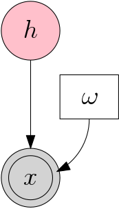
Fig. 5 shows the representation of a generative graphical model that produces observations x𝑥x from a distribution xpω(x|h)similar-to𝑥subscript𝑝𝜔conditional𝑥x\sim p_{\omega}(x|h), has hidden variables hh, and is parameterised by a set of parameters, ω𝜔\omega. In learning a model, we often seek the parameters that maximises the log-marginal-likelihood (LML), which can be found by marginalising the joint distribution pω(x,h)subscript𝑝𝜔𝑥p_{\omega}(x,h) over hidden variables:

Refer to caption
Figure 5: Graphical model of inference problem.
ω(x)logpω(x)=log(pω(x,h)𝑑h).subscript𝜔𝑥subscript𝑝𝜔𝑥subscriptsubscript𝑝𝜔𝑥differential-d\displaystyle\ell_{\omega}(x)\coloneqq\log p_{\omega}(x)=\log\left(\int_{\mathcal{H}}p_{\omega}(x,h)dh\right). (12)

In many cases, we also need to infer the corresponding posterior,

pω(h|x)=pω(x,h)pω(x,h)𝑑h.subscript𝑝𝜔conditional𝑥subscript𝑝𝜔𝑥subscriptsubscript𝑝𝜔𝑥differential-d\displaystyle p_{\omega}(h|x)=\frac{p_{\omega}(x,h)}{\int_{\mathcal{H}}p_{\omega}(x,h)dh}. (13)

Evaluating the marginal likelihood in Eq. 12 and obtain the corresponding posterior, however, is intractable for most distributions. To compute the marginal likelihood and ωsuperscript𝜔\omega^{*}, we can use the EM algorithm [13] and variational inference (VI). We review these two methods now.

For any valid probability distribution q(h)𝑞q(h) with support over hh we can rewrite the LML as a difference of two divergences [29],

ω(x)=subscript𝜔𝑥absent\displaystyle\ell_{\omega}(x)= q(h)log(pω(x,h)q(h))𝑑hq(h)log(pω(h|x)q(h))𝑑h,subscript𝑞subscript𝑝𝜔𝑥𝑞differential-dsubscript𝑞subscript𝑝𝜔conditional𝑥𝑞differential-d\displaystyle\int_{\mathcal{H}}q(h)\log\left(\frac{p_{\omega}(x,h)}{q(h)}\right)dh-\int_{\mathcal{H}}q(h)\log\left(\frac{p_{\omega}(h|x)}{q(h)}\right)dh, (14)
=\displaystyle= (ω,q(h))+KL(q(h)pω(h|x)),\displaystyle\mathcal{L}(\omega,q(h))+\textsc{KL}(q(h)\;\|\;p_{\omega}(h|x)), (15)

where (ω,q(h))q(h)log(pω(x,h)q(h))𝑑h𝜔𝑞subscript𝑞subscript𝑝𝜔𝑥𝑞differential-d\mathcal{L}(\omega,q(h))\coloneqq\int_{\mathcal{H}}q(h)\log\left(\frac{p_{\omega}(x,h)}{q(h)}\right)dh is known as the evidence lower bound (ELBO). Intuitively, as KL(q(h)pω(h|x))0\textsc{KL}(q(h)\;\|\;p_{\omega}(h|x))\geq 0, it follows that ω(x)ELBO(q(h);ω)subscript𝜔𝑥ELBO𝑞𝜔\ell_{\omega}(x)\geq\textsc{ELBO}\left(q(h);\omega\right), hence ω(x)ELBO(q(h);ω)subscript𝜔𝑥ELBO𝑞𝜔\ell_{\omega}(x)\geq\textsc{ELBO}\left(q(h);\omega\right) is a lower bound for the LML. The derivation of this bound can also be viewed as applying Jensen’s inequality directly to Eq. 12 [8]. Note that when the ELBO and marginal likelihood are identical, the resulting KL divergence between the function q(h)𝑞q(h) and the posterior p(h|x)𝑝conditional𝑥p(h|x) is zero, implying that q(h)=pω(h|x)𝑞subscript𝑝𝜔conditional𝑥q(h)=p_{\omega}(h|x).

Maximising the LML now reduces to maximising the ELBO, which can be achieved iteratively using EM [13, 70]; an expectation step (E-step) finds the posterior for the current set of model parameters and then a maximisation step (M-step) maximises the ELBO with respect to ω𝜔\omega while keeping q(h)𝑞q(h) fixed as the posterior from the E-step.

As finding the exact posterior in the E-step is still typically intractable, we resort to variational inference (VI), a powerful tool for approximating the posterior using a parametrised variational distribution qθ(h)subscript𝑞𝜃q_{\theta}(h) [29, 4]. VI aims to reduce the KL divergence between the true posterior and the variational distribution, KL(qθ(h)pω(h|x))\textsc{KL}(q_{\theta}(h)\;\|\;p_{\omega}(h|x)). Typically VI never brings this divergence to zero but nonetheless yields useful posterior approximations. As minimising KL(qθ(h)pω(h|x))\textsc{KL}(q_{\theta}(h)\;\|\;p_{\omega}(h|x)) is equivalent to maximising the ELBO for the variational distribution (see Eq. 116 from Theorem 3), the variational E-step amounts to maximising the ELBO with respect to θ𝜃\theta while keeping ω𝜔\omega constant. The variational EM algorithm can be summarised as:

Variational E-Step: θk+1argmaxθ(ωk,θ),subscript𝜃𝑘1subscriptargmax𝜃subscript𝜔𝑘𝜃\displaystyle\theta_{k+1}\leftarrow\operatorname*{arg\,max}_{\theta}\mathcal{L}(\omega_{k},\theta), (16)
Variational M-Step: ωk+1argmaxω(ω,θk+1).subscript𝜔𝑘1subscriptargmax𝜔𝜔subscript𝜃𝑘1\displaystyle\omega_{k+1}\leftarrow\operatorname*{arg\,max}_{\omega}\mathcal{L}(\omega,\theta_{k+1}). (17)

Appendix B A Probabilistic Interpretation of virel

We now motivate our inference procedure and Boltzmann distribution πω(a|s)subscript𝜋𝜔conditional𝑎𝑠\pi_{\omega}(a|s) from a probabilistic perspective, demonstrating that πω(a|s)subscript𝜋𝜔conditional𝑎𝑠\pi_{\omega}(a|s) can be interpreted as an action-posterior that characterises the uncertainty our model has in the optimality of Q^ω(h)subscript^𝑄𝜔\hat{Q}_{\omega}(h). Moreover, maximising (ω,θ)𝜔𝜃\mathcal{L}(\omega,\theta) for θ𝜃\theta is equivalent to carrying our variational inference on the graphical model in Fig. 6 for any εω>0subscript𝜀𝜔0\varepsilon_{\omega}>0.

B.1 Model Specification

Like previous work, we introduce a binary variable 𝒪{0,1}𝒪01\mathcal{O}\in\{0,1\} in order to define a formal graphical model for our inference problem when εω>0subscript𝜀𝜔0\varepsilon_{\omega}>0. The likelihood of 𝒪𝒪\mathcal{O} therefore takes the form of a Bernoulli distribution:

pω(𝒪|h)=yω(h)𝒪(1yω(h))(1𝒪),subscript𝑝𝜔conditional𝒪subscript𝑦𝜔superscript𝒪superscript1subscript𝑦𝜔1𝒪\displaystyle p_{\omega}(\mathcal{O}|h)=y_{\omega}(h)^{\mathcal{O}}(1-y_{\omega}(h))^{(1-\mathcal{O})}, (18)

where

yω(h)exp(Q^ω(h)maxaQ^ω(a,s)εω).subscript𝑦𝜔subscript^𝑄𝜔subscriptsuperscript𝑎subscript^𝑄𝜔superscript𝑎𝑠subscript𝜀𝜔\displaystyle y_{\omega}(h)\coloneqq\exp\left(\frac{\hat{Q}_{\omega}(h)-\max_{a^{\prime}}\hat{Q}_{\omega}(a^{\prime},s)}{\varepsilon_{\omega}}\right). (19)

In most existing frameworks, 𝒪=1𝒪1\mathcal{O}=1 is understood to be the event that the agent is acting optimally [34, 62]. As we are using function approximators in virel, 𝒪=1𝒪1\mathcal{O}=1 can be interpreted as the event that the agent is behaving optimally under Q^ω(h)subscript^𝑄𝜔\hat{Q}_{\omega}(h). Exploring the semantics of 𝒪𝒪\mathcal{O} further, consider the likelihood when 𝒪=1𝒪1\mathcal{O}=1:

pω(𝒪=1|h)=exp(Q^ω(h)maxaQ^ω(a,s)εω),subscript𝑝𝜔𝒪conditional1subscript^𝑄𝜔subscriptsuperscript𝑎subscript^𝑄𝜔superscript𝑎𝑠subscript𝜀𝜔\displaystyle p_{\omega}(\mathcal{O}=1|h)=\exp\left(\frac{\hat{Q}_{\omega}(h)-\max_{a^{\prime}}\hat{Q}_{\omega}(a^{\prime},s)}{\varepsilon_{\omega}}\right), (20)
Refer to caption
Figure 6: Graphical model for virel (variational approximation dashed)

Observe that 0pω(𝒪=1|)10subscript𝑝𝜔𝒪conditional110\leq p_{\omega}(\mathcal{O}=1|\cdot)\leq 1 ωΩs.t.εω>0formulae-sequencefor-all𝜔Ω𝑠𝑡subscript𝜀𝜔0\forall\ \omega\in\Omega\ s.t.\ \varepsilon_{\omega}>0. For any state s𝑠s and any action asuperscript𝑎a^{*} such that pω(𝒪=1|s,a)=1subscript𝑝𝜔𝒪conditional1𝑠superscript𝑎1p_{\omega}(\mathcal{O}=1|s,a^{*})=1, such an action must be optimal under Q^ω(h)subscript^𝑄𝜔\hat{Q}_{\omega}(h) in the sense that it is the greedy action aargmaxaQ^ω(h)superscript𝑎subscriptargmax𝑎subscript^𝑄𝜔a^{*}\in\operatorname*{arg\,max}_{a}\hat{Q}_{\omega}(h). If we find pω(𝒪=1|h)=1hsubscript𝑝𝜔𝒪conditional11for-allp_{\omega}(\mathcal{O}=1|h)=1\ \forall\ h\in\mathcal{H}, then all observed state-action pairs have been generated from a greedy policy π(a|s)=δ(aargmaxaQ^ω(a|s))𝜋conditional𝑎𝑠𝛿𝑎subscriptargmaxsuperscript𝑎subscript^𝑄𝜔conditionalsuperscript𝑎𝑠\pi(a|s)=\delta(a\in\operatorname*{arg\,max}_{a^{\prime}}\hat{Q}_{\omega}(a^{\prime}|s)). From Theorem 2, the closer the residual error εωsubscript𝜀𝜔\varepsilon_{\omega} is to zero, the closer Q^ω(h)subscript^𝑄𝜔\hat{Q}_{\omega}(h) becomes to representing an optimal action-value function. When εω0subscript𝜀𝜔0\varepsilon_{\omega}\approx 0, any a𝑎a observed such that pω(𝒪=1|a,)=1subscript𝑝𝜔𝒪conditional1𝑎1p_{\omega}(\mathcal{O}=1|a,\cdot)=1 will be very nearly an action sampled from an optimal policy, that is aπ(a|)δ(aargmaxaQ(a|))similar-to𝑎𝜋conditional𝑎𝛿𝑎subscriptargmaxsuperscript𝑎superscript𝑄conditionalsuperscript𝑎a\sim\pi(a|\cdot)\approx\delta(a\in\operatorname*{arg\,max}_{a^{\prime}}Q^{*}(a^{\prime}|\cdot)). We caution readers that in the limit εω0subscript𝜀𝜔0\varepsilon_{\omega}\rightarrow 0, our likelihood is not well-defined for any aargmaxaQ^ω(a,s)𝑎subscriptargmaxsuperscript𝑎subscript^𝑄𝜔superscript𝑎𝑠a\in\operatorname*{arg\,max}_{a^{\prime}}\hat{Q}_{\omega}(a^{\prime},s). Without loss of generality, we condition on optimality for the rest of this section, writing 𝒪𝒪\mathcal{O} in place of 𝒪=1𝒪1\mathcal{O}=1. Defining the function yω(s)exp(maxaQ^ω(a,s)εω)subscript𝑦𝜔𝑠subscriptsuperscript𝑎subscript^𝑄𝜔superscript𝑎𝑠subscript𝜀𝜔y_{\omega}(s)\coloneqq\exp\left(-\frac{\max_{a^{\prime}}\hat{Q}_{\omega}(a^{\prime},s)}{\varepsilon_{\omega}}\right), our likelihood takes the convenient form:

pω(𝒪|h)=exp(Q^ω(h)εω)yω(s),subscript𝑝𝜔conditional𝒪subscript^𝑄𝜔subscript𝜀𝜔subscript𝑦𝜔𝑠\displaystyle p_{\omega}(\mathcal{O}|h)=\exp\left(\frac{\hat{Q}_{\omega}(h)}{\varepsilon_{\omega}}\right)y_{\omega}(s), (21)

Defining the prior distribution as the uniform distribution p(h)=𝒰(h)𝑝𝒰p(h)=\mathcal{U}(h) completes our model, the graph for which is shown in Fig. 6. Using Bayes’ rule, we find our posterior distribution is:

pω(h|𝒪)subscript𝑝𝜔conditional𝒪\displaystyle p_{\omega}(h|\mathcal{O}) =pω(𝒪|h)p(h)pω(𝒪),absentsubscript𝑝𝜔conditional𝒪𝑝subscript𝑝𝜔𝒪\displaystyle=\frac{p_{\omega}(\mathcal{O}|h)p(h)}{p_{\omega}(\mathcal{O})}, (22)
=pω(𝒪|h)p(h)pω(𝒪|h)p(h)𝑑h,absentsubscript𝑝𝜔conditional𝒪𝑝subscriptsubscript𝑝𝜔conditional𝒪𝑝differential-d\displaystyle=\frac{p_{\omega}(\mathcal{O}|h)p(h)}{\int_{\mathcal{H}}p_{\omega}(\mathcal{O}|h)p(h)dh}, (23)
=exp(Q^ω(h)εω)yω(s)exp(Q^ω(h)εω)yω(s)𝑑h.absentsubscript^𝑄𝜔subscript𝜀𝜔subscript𝑦𝜔𝑠subscriptsubscript^𝑄𝜔subscript𝜀𝜔subscript𝑦𝜔𝑠differential-d\displaystyle=\frac{\exp\left(\frac{\hat{Q}_{\omega}(h)}{\varepsilon_{\omega}}\right)y_{\omega}(s)}{\int_{\mathcal{H}}\exp\left(\frac{\hat{Q}_{\omega}(h)}{\varepsilon_{\omega}}\right)y_{\omega}(s)dh}. (24)

We can also derive our action-posterior, pω(a|s,𝒪)subscript𝑝𝜔conditional𝑎𝑠𝒪p_{\omega}(a|s,\mathcal{O}), which we will find to be equivalent to the Boltzmann policy from Eq. 5. Using Bayes’ rule, it follows:

pω(a|s,𝒪)subscript𝑝𝜔conditional𝑎𝑠𝒪\displaystyle p_{\omega}(a|s,\mathcal{O}) =pω(h|𝒪)pω(s|𝒪).absentsubscript𝑝𝜔conditional𝒪subscript𝑝𝜔conditional𝑠𝒪\displaystyle=\frac{p_{\omega}(h|\mathcal{O})}{p_{\omega}(s|\mathcal{O})}. (25)

Now, we find pω(s|𝒪)subscript𝑝𝜔conditional𝑠𝒪p_{\omega}(s|\mathcal{O}) by marginalising our posterior over actions. Substituting pω(s|𝒪)=pω(h|𝒪)𝑑asubscript𝑝𝜔conditional𝑠𝒪subscript𝑝𝜔conditional𝒪differential-d𝑎p_{\omega}(s|\mathcal{O})=\int p_{\omega}(h|\mathcal{O})da yields :

pω(a|s,𝒪)subscript𝑝𝜔conditional𝑎𝑠𝒪\displaystyle p_{\omega}(a|s,\mathcal{O}) =pω(h|𝒪)𝒜pω(h|𝒪)𝑑a.absentsubscript𝑝𝜔conditional𝒪subscript𝒜subscript𝑝𝜔conditional𝒪differential-d𝑎\displaystyle=\frac{p_{\omega}(h|\mathcal{O})}{\int_{\mathcal{A}}p_{\omega}(h|\mathcal{O})da}. (26)

Substituting for our posterior from Eq. 24, we obtain:

pω(a|s,𝒪)subscript𝑝𝜔conditional𝑎𝑠𝒪\displaystyle p_{\omega}(a|s,\mathcal{O}) =exp(Q^ω(h)εω)yω(s)𝒜exp(Q^ω(h)εω)yω(s)𝑑aexp(Q^ω(h)εω)yω(s)𝑑hexp(Q^ω(h)εω)yω(s)𝑑h,absentsubscript^𝑄𝜔subscript𝜀𝜔subscript𝑦𝜔𝑠subscript𝒜subscript^𝑄𝜔subscript𝜀𝜔subscript𝑦𝜔𝑠differential-d𝑎subscriptsubscript^𝑄𝜔subscript𝜀𝜔subscript𝑦𝜔𝑠differential-dsubscriptsubscript^𝑄𝜔subscript𝜀𝜔subscript𝑦𝜔𝑠differential-d\displaystyle=\frac{\exp\left(\frac{\hat{Q}_{\omega}(h)}{\varepsilon_{\omega}}\right)y_{\omega}(s)}{\int_{\mathcal{A}}\exp\left(\frac{\hat{Q}_{\omega}(h)}{\varepsilon_{\omega}}\right)y_{\omega}(s)da}\cdot\frac{\int_{\mathcal{H}}\exp\left(\frac{\hat{Q}_{\omega}(h)}{\varepsilon_{\omega}}\right)y_{\omega}(s)dh}{\int_{\mathcal{H}}\exp\left(\frac{\hat{Q}_{\omega}(h)}{\varepsilon_{\omega}}\right)y_{\omega}(s)dh}, (27)
=exp(Q^ω(h)εω)yω(s)(𝒜exp(Q^ω(h)εω)𝑑a)yω(s),absentsubscript^𝑄𝜔subscript𝜀𝜔subscript𝑦𝜔𝑠subscript𝒜subscript^𝑄𝜔subscript𝜀𝜔differential-d𝑎subscript𝑦𝜔𝑠\displaystyle=\frac{\exp\left(\frac{\hat{Q}_{\omega}(h)}{\varepsilon_{\omega}}\right)y_{\omega}(s)}{\left(\int_{\mathcal{A}}\exp\left(\frac{\hat{Q}_{\omega}(h)}{\varepsilon_{\omega}}\right)da\right)y_{\omega}(s)}, (28)
=exp(Q^ω(h)εω)𝒜exp(Q^ω(h)εω)𝑑a,absentsubscript^𝑄𝜔subscript𝜀𝜔subscript𝒜subscript^𝑄𝜔subscript𝜀𝜔differential-d𝑎\displaystyle=\frac{\exp\left(\frac{\hat{Q}_{\omega}(h)}{\varepsilon_{\omega}}\right)}{\int_{\mathcal{A}}\exp\left(\frac{\hat{Q}_{\omega}(h)}{\varepsilon_{\omega}}\right)da}, (29)
=πω(a|s),absentsubscript𝜋𝜔conditional𝑎𝑠\displaystyle=\pi_{\omega}(a|s), (30)

proving that our action-posterior is exactly the Boltzmann policy introduced in Section 3.1. From a Bayesian perspective, the action-posterior pω(a|s,𝒪)subscript𝑝𝜔conditional𝑎𝑠𝒪p_{\omega}(a|s,\mathcal{O}) characterises the uncertainty we have in deducing the optimal action for a given state s𝑠s under Q^ω(h)subscript^𝑄𝜔\hat{Q}_{\omega}(h); whenever εω0subscript𝜀𝜔0\varepsilon_{\omega}\approx 0 and hence Q^ω(h)Q(h)subscript^𝑄𝜔superscript𝑄\hat{Q}_{\omega}(h)\approx Q^{*}(h), the uncertainty will be very small as pω(a|s,𝒪)subscript𝑝𝜔conditional𝑎𝑠𝒪p_{\omega}(a|s,\mathcal{O}) will have near-zero variance, approximating a Dirac-delta distribution. Our model is therefore highly confident that the maximum-a-posteriori (MAP) action aargmaxaQ^ω(a,s)𝑎subscriptargmaxsuperscript𝑎subscript^𝑄𝜔superscript𝑎𝑠a\in\operatorname*{arg\,max}_{a^{\prime}}\hat{Q}_{\omega}(a^{\prime},s) is an optimal action, with all of the probability mass being close to this point. In light of this, we can interpret the greedy policy πω(a|s)=δ(aargmaxaQ^ω(a,s))subscript𝜋𝜔conditional𝑎𝑠𝛿𝑎subscriptargmaxsuperscript𝑎subscript^𝑄𝜔superscript𝑎𝑠\pi_{\omega}(a|s)=\delta(a\in\operatorname*{arg\,max}_{a^{\prime}}\hat{Q}_{\omega}(a^{\prime},s)) as one that always selecting the MAP action across all states.

As our model incorporates the uncertainty in the optimality of Q^ω(h)subscript^𝑄𝜔\hat{Q}_{\omega}(h) into the variance of πω(a|s)subscript𝜋𝜔conditional𝑎𝑠\pi_{\omega}(a|s), we can benefit directly by sampling trajectories from πω(a|s)subscript𝜋𝜔conditional𝑎𝑠\pi_{\omega}(a|s) which drives exploration to gather data that is beneficial to reducing the residual error εωsubscript𝜀𝜔\varepsilon_{\omega}. Unfortunately, calculating the normalisation constant 𝒜exp(Q^ω(h)εω)𝑑asubscript𝒜subscript^𝑄𝜔subscript𝜀𝜔differential-d𝑎\int_{\mathcal{A}}\exp\left(\frac{\hat{Q}_{\omega}(h)}{\varepsilon_{\omega}}\right)da is intractable for most function approximators and MDPs of interest. As such, we resort to variational inference, a powerful technique to infer an approximation to a posterior distribution from a tractable family of variational distributions [29, 4, 8]. As before πθ(a|s)subscript𝜋𝜃conditional𝑎𝑠\pi_{\theta}(a|s) is known as the variational policy, is parametrised by θΘ𝜃Θ\theta\in\Theta and with the same support as πω(a|s)subscript𝜋𝜔conditional𝑎𝑠\pi_{\omega}(a|s). Like in Section 3.1, we define a variational distribution as qθ(h)d(s)πθ(a|s)subscript𝑞𝜃𝑑𝑠subscript𝜋𝜃conditional𝑎𝑠q_{\theta}(h)\coloneqq d(s)\pi_{\theta}(a|s), where d(s)𝑑𝑠d(s) is an arbitrary sampling distribution with support over 𝒮𝒮\mathcal{S}. We fix d(s)𝑑𝑠d(s), as in our model-free paradigm we do not learn the state transition dynamics and only seek to infer the action-posterior.

The goal of variational inference is to find qθ(h)subscript𝑞𝜃q_{\theta}(h) closest in KL-divergence to pω(h|𝒪)subscript𝑝𝜔conditional𝒪p_{\omega}(h|\mathcal{O}), giving an objective:

θargminθKL(qθ(h)pω(h|𝒪)).\displaystyle\theta^{*}\in\operatorname*{arg\,min}_{\theta}\textsc{KL}(q_{\theta}(h)\;\|\;p_{\omega}(h|\mathcal{O})). (31)

This objective still requires the intractable computation of exp(Q^ω(h)εω)yω(s)𝑑hsubscript^𝑄𝜔subscript𝜀𝜔subscript𝑦𝜔𝑠differential-d\int\exp\left(\frac{\hat{Q}_{\omega}(h)}{\varepsilon_{\omega}}\right)y_{\omega}(s)dh. Using Eq. 15, we can overcome this by writing the KL divergence in terms of the ELBO:

KL(qθ(h)pω(h|𝒪))=ωω(θ),\displaystyle\textsc{KL}(q_{\theta}(h)\;\|\;p_{\omega}(h|\mathcal{O}))=\ell_{\omega}-\mathcal{L}_{\omega}(\theta), (32)
whereωlogexp(Q^ω(h)εω)yω(s)𝑑h,ω(θ)𝔼hqθ(h)[log(exp(Q^ω(h)εω)yω(s)qθ(h))].formulae-sequencewheresubscript𝜔subscriptsubscript^𝑄𝜔subscript𝜀𝜔subscript𝑦𝜔𝑠differential-dsubscript𝜔𝜃subscript𝔼similar-tosubscript𝑞𝜃delimited-[]subscript^𝑄𝜔subscript𝜀𝜔subscript𝑦𝜔𝑠subscript𝑞𝜃\displaystyle\mathrm{where}\quad\ell_{\omega}\coloneqq\log\int_{\mathcal{H}}\exp\left(\frac{\hat{Q}_{\omega}(h)}{\varepsilon_{\omega}}\right)y_{\omega}(s)dh,\quad\mathcal{L}_{\omega}(\theta)\coloneqq\mathbb{E}_{h\sim q_{\theta}(h)}\left[\log\left(\frac{\exp\left(\frac{\hat{Q}_{\omega}(h)}{\varepsilon_{\omega}}\right)y_{\omega}(s)}{q_{\theta}(h)}\right)\right]. (33)

We see that minimising the KL-divergence for θ𝜃\theta is equivalent to maximising the ELBO for θ𝜃\theta, which is tractable. This affords a new objective:

θargmaxθω(θ).superscript𝜃subscriptargmax𝜃subscript𝜔𝜃\displaystyle\theta^{*}\in\operatorname*{arg\,max}_{\theta}\mathcal{L}_{\omega}(\theta). (34)

Expanding the ELBO yields:

ω(θ)subscript𝜔𝜃\displaystyle\mathcal{L}_{\omega}(\theta) =𝔼hqθ(h)[log(exp(Q^ω(h)εω)yω(s)qθ(h))],absentsubscript𝔼similar-tosubscript𝑞𝜃delimited-[]subscript^𝑄𝜔subscript𝜀𝜔subscript𝑦𝜔𝑠subscript𝑞𝜃\displaystyle=\mathbb{E}_{h\sim q_{\theta}(h)}\left[\log\left(\frac{\exp\left(\frac{\hat{Q}_{\omega}(h)}{\varepsilon_{\omega}}\right)y_{\omega}(s)}{q_{\theta}(h)}\right)\right], (35)
=𝔼sd(s)[𝔼aπθ(a|s)[log(exp(Q^ω(h)εω)yω(s)qθ(h))]],absentsubscript𝔼similar-to𝑠𝑑𝑠delimited-[]subscript𝔼similar-to𝑎subscript𝜋𝜃conditional𝑎𝑠delimited-[]subscript^𝑄𝜔subscript𝜀𝜔subscript𝑦𝜔𝑠subscript𝑞𝜃\displaystyle=\mathbb{E}_{s\sim d(s)}\left[\mathbb{E}_{a\sim\pi_{\theta}(a|s)}\left[\log\left(\frac{\exp\left(\frac{\hat{Q}_{\omega}(h)}{\varepsilon_{\omega}}\right)y_{\omega}(s)}{q_{\theta}(h)}\right)\right]\right], (36)
=𝔼sd(s)[𝔼aπθ(a|s)[Q^ω(h)εω]+𝔼aπθ(a|s)[logyω(s)]𝔼aπθ(a|s)[log(πθ(a|s)d(s))]],absentsubscript𝔼similar-to𝑠𝑑𝑠delimited-[]subscript𝔼similar-to𝑎subscript𝜋𝜃conditional𝑎𝑠delimited-[]subscript^𝑄𝜔subscript𝜀𝜔subscript𝔼similar-to𝑎subscript𝜋𝜃conditional𝑎𝑠delimited-[]subscript𝑦𝜔𝑠subscript𝔼similar-to𝑎subscript𝜋𝜃conditional𝑎𝑠delimited-[]subscript𝜋𝜃conditional𝑎𝑠𝑑𝑠\displaystyle=\mathbb{E}_{s\sim d(s)}\left[\mathbb{E}_{a\sim\pi_{\theta}(a|s)}\left[\frac{\hat{Q}_{\omega}(h)}{\varepsilon_{\omega}}\right]+\mathbb{E}_{a\sim\pi_{\theta}(a|s)}\left[\log y_{\omega}(s)\right]-\mathbb{E}_{a\sim\pi_{\theta}(a|s)}\left[\log(\pi_{\theta}(a|s)d(s))\right]\right], (37)
=𝔼sd(s)[𝔼aπθ(a|s)[Q^ω(h)εω]+logyω(s)logd(s)𝔼aπθ(a|s)[logπθ(a|s)]],absentsubscript𝔼similar-to𝑠𝑑𝑠delimited-[]subscript𝔼similar-to𝑎subscript𝜋𝜃conditional𝑎𝑠delimited-[]subscript^𝑄𝜔subscript𝜀𝜔subscript𝑦𝜔𝑠𝑑𝑠subscript𝔼similar-to𝑎subscript𝜋𝜃conditional𝑎𝑠delimited-[]subscript𝜋𝜃conditional𝑎𝑠\displaystyle=\mathbb{E}_{s\sim d(s)}\left[\mathbb{E}_{a\sim\pi_{\theta}(a|s)}\left[\frac{\hat{Q}_{\omega}(h)}{\varepsilon_{\omega}}\right]+\log y_{\omega}(s)-\log d(s)-\mathbb{E}_{a\sim\pi_{\theta}(a|s)}\left[\log\pi_{\theta}(a|s)\right]\right], (38)
=𝔼sd(s)[𝔼aπθ(a|s)[Q^ω(h)εω]𝔼aπθ(a|s)[logπθ(a|s)]]+𝔼sd(s)[log(yω(s)d(s))],absentsubscript𝔼similar-to𝑠𝑑𝑠delimited-[]subscript𝔼similar-to𝑎subscript𝜋𝜃conditional𝑎𝑠delimited-[]subscript^𝑄𝜔subscript𝜀𝜔subscript𝔼similar-to𝑎subscript𝜋𝜃conditional𝑎𝑠delimited-[]subscript𝜋𝜃conditional𝑎𝑠subscript𝔼similar-to𝑠𝑑𝑠delimited-[]subscript𝑦𝜔𝑠𝑑𝑠\displaystyle=\mathbb{E}_{s\sim d(s)}\left[\mathbb{E}_{a\sim\pi_{\theta}(a|s)}\left[\frac{\hat{Q}_{\omega}(h)}{\varepsilon_{\omega}}\right]-\mathbb{E}_{a\sim\pi_{\theta}(a|s)}\left[\log\pi_{\theta}(a|s)\right]\right]+\mathbb{E}_{s\sim d(s)}\left[\log\left(\frac{y_{\omega}(s)}{d(s)}\right)\right], (39)
=𝔼sd(s)[𝔼aπθ(a|s)[Q^ω(h)εω]+(πθ(a|s))]+𝔼sd(s)[log(yω(s)d(s))].absentsubscript𝔼similar-to𝑠𝑑𝑠delimited-[]subscript𝔼similar-to𝑎subscript𝜋𝜃conditional𝑎𝑠delimited-[]subscript^𝑄𝜔subscript𝜀𝜔subscript𝜋𝜃conditional𝑎𝑠subscript𝔼similar-to𝑠𝑑𝑠delimited-[]subscript𝑦𝜔𝑠𝑑𝑠\displaystyle=\mathbb{E}_{s\sim d(s)}\left[\mathbb{E}_{a\sim\pi_{\theta}(a|s)}\left[\frac{\hat{Q}_{\omega}(h)}{\varepsilon_{\omega}}\right]+\mathscr{H}(\pi_{\theta}(a|s))\right]+\mathbb{E}_{s\sim d(s)}\left[\log\left(\frac{y_{\omega}(s)}{d(s)}\right)\right]. (40)

As the final term 𝔼sd(s)[log(yω(s)d(s))]subscript𝔼similar-to𝑠𝑑𝑠delimited-[]subscript𝑦𝜔𝑠𝑑𝑠\mathbb{E}_{s\sim d(s)}\left[\log\left(\frac{y_{\omega}(s)}{d(s)}\right)\right] has no dependency on θ𝜃\theta, we can neglect it from our objective, recovering the virel objective from Eq. 6:

ω(θ)subscript𝜔𝜃\displaystyle\mathcal{L}_{\omega}(\theta) =𝔼sd(s)[𝔼aπθ(a|s)[Q^ω(h)εω]+(πθ(a|s))].absentsubscript𝔼similar-to𝑠𝑑𝑠delimited-[]subscript𝔼similar-to𝑎subscript𝜋𝜃conditional𝑎𝑠delimited-[]subscript^𝑄𝜔subscript𝜀𝜔subscript𝜋𝜃conditional𝑎𝑠\displaystyle=\mathbb{E}_{s\sim d(s)}\left[\mathbb{E}_{a\sim\pi_{\theta}(a|s)}\left[\frac{\hat{Q}_{\omega}(h)}{\varepsilon_{\omega}}\right]+\mathscr{H}(\pi_{\theta}(a|s))\right]. (41)

Finally, Theorem 3 guarantees that minimising ω(θ)subscript𝜔𝜃\mathcal{L}_{\omega}(\theta) always minimises the expected KL divergence between πω(a|s)subscript𝜋𝜔conditional𝑎𝑠\pi_{\omega}(a|s) and πθ(a|s)subscript𝜋𝜃conditional𝑎𝑠\pi_{\theta}(a|s), allowing us to learn a variational approximation for the action-posterior.

Appendix C A Discussion of the Target Set 𝕋𝕋\mathbb{T}

We now prove that the Bellman operator for the Boltzmann policy, 𝒯πωr(h)+γ𝔼hp(s|h)πω(a|s)[]\mathcal{T}^{\pi_{\omega}}\bm{\cdot}\coloneqq r(h)+\gamma\mathbb{E}_{h^{\prime}\sim p(s^{\prime}|h)\pi_{\omega}(a^{\prime}|s^{\prime})}\left[\bm{\cdot}\right], is a member of 𝕋𝕋\mathbb{T}. Taking the limit εω0subscript𝜀𝜔0\varepsilon_{\omega}\rightarrow 0 of 𝒯πωQ^ω(h)superscript𝒯subscript𝜋𝜔subscript^𝑄𝜔\mathcal{T}^{\pi_{\omega}}\hat{Q}_{\omega}(h), we find:

limεω0𝒯πωQ^ω(h)subscriptsubscript𝜀𝜔0superscript𝒯subscript𝜋𝜔subscript^𝑄𝜔\displaystyle\lim_{\varepsilon_{\omega}\rightarrow 0}\mathcal{T}^{\pi_{\omega}}\hat{Q}_{\omega}(h) =r(h)+limεω0γ𝔼hp(s|h)πω(a|s)[Q^ω(h)].absent𝑟subscriptsubscript𝜀𝜔0𝛾subscript𝔼similar-tosuperscript𝑝conditionalsuperscript𝑠subscript𝜋𝜔conditionalsuperscript𝑎superscript𝑠delimited-[]subscript^𝑄𝜔superscript\displaystyle=r(h)+\lim_{\varepsilon_{\omega}\rightarrow 0}\gamma\mathbb{E}_{h^{\prime}\sim p(s^{\prime}|h)\pi_{\omega}(a^{\prime}|s^{\prime})}\left[\hat{Q}_{\omega}(h^{\prime})\right]. (42)

From Theorem 2, evalutating limεω0γ𝔼hp(s|h)πω(a|s)[]subscriptsubscript𝜀𝜔0𝛾subscript𝔼similar-tosuperscript𝑝conditionalsuperscript𝑠subscript𝜋𝜔conditionalsuperscript𝑎superscript𝑠delimited-[]bold-⋅\lim_{\varepsilon_{\omega}\rightarrow 0}\gamma\mathbb{E}_{h^{\prime}\sim p(s^{\prime}|h)\pi_{\omega}(a^{\prime}|s^{\prime})}\left[\bm{\cdot}\right] recovers a Dirac-delta distribution:

limεω0𝒯πωQ^ω(h)subscriptsubscript𝜀𝜔0superscript𝒯subscript𝜋𝜔subscript^𝑄𝜔\displaystyle\lim_{\varepsilon_{\omega}\rightarrow 0}\mathcal{T}^{\pi_{\omega}}\hat{Q}_{\omega}(h) =r(h)+γ𝔼hp(s|h)δ(a=argmaxaQ^ω(a,s))[Q^ω(h)],absent𝑟𝛾subscript𝔼similar-tosuperscript𝑝conditionalsuperscript𝑠𝛿superscript𝑎subscriptargmax𝑎subscript^𝑄𝜔𝑎𝑠delimited-[]subscript^𝑄𝜔superscript\displaystyle=r(h)+\gamma\mathbb{E}_{h^{\prime}\sim p(s^{\prime}|h)\delta(a^{\prime}=\operatorname*{arg\,max}_{a}\hat{Q}_{\omega}(a,s))}\left[\hat{Q}_{\omega}(h^{\prime})\right], (43)
=r(h)+γ𝔼hp(s|h)[maxa(Q^ω(h))],absent𝑟𝛾subscript𝔼similar-tosuperscript𝑝conditionalsuperscript𝑠delimited-[]subscriptsuperscript𝑎subscript^𝑄𝜔superscript\displaystyle=r(h)+\gamma\mathbb{E}_{h^{\prime}\sim p(s^{\prime}|h)}\left[\max_{a^{\prime}}(\hat{Q}_{\omega}(h^{\prime}))\right], (44)
=𝒯Q^ω(h).absentsuperscript𝒯subscript^𝑄𝜔\displaystyle=\mathcal{T}^{*}\hat{Q}_{\omega}(h). (45)

which is sufficient to demonstrate membership of 𝕋𝕋\mathbb{T}.

Observe that using 𝒯πω\mathcal{T}^{\pi_{\omega}}\bm{\cdot} implies Q^ω(h)subscript^𝑄𝜔\hat{Q}_{\omega}(h) cannot represent the true Q𝑄Q-function of any πω(a|s)subscript𝜋𝜔conditional𝑎𝑠\pi_{\omega}(a|s) except for the optimal Q-function. To see this, imagine there exists some εω>0subscript𝜀𝜔0\varepsilon_{\omega}>0 such that Qπω()=Q^()superscript𝑄subscript𝜋𝜔^𝑄Q^{\pi_{\omega}}(\cdot)=\hat{Q}(\cdot). Under these conditions, it holds that 𝒯πωQ^()=Q^()εω=0superscript𝒯subscript𝜋𝜔^𝑄^𝑄subscript𝜀𝜔0\mathcal{T}^{\pi_{\omega}}\hat{Q}(\cdot)=\hat{Q}(\cdot)\implies\varepsilon_{\omega}=0, which is a contradiction. More generally, as πω(a|s)subscript𝜋𝜔conditional𝑎𝑠\pi_{\omega}(a|s) is defined in terms of εωsubscript𝜀𝜔\varepsilon_{\omega}, which itself depends on πω(a|s)subscript𝜋𝜔conditional𝑎𝑠\pi_{\omega}(a|s) from the definition of 𝒯πω\mathcal{T}^{\pi_{\omega}}\bm{\cdot}, any ω𝜔\omega satisfying this recursive definition forms a constrained set ΩcΩsuperscriptΩ𝑐Ω\Omega^{c}\subseteq\Omega. Crucially, we show in Theorem 2 that there always exists some ωΩcsuperscript𝜔superscriptΩ𝑐\omega^{*}\in\Omega^{c} such that Q^ωsubscript^𝑄superscript𝜔\hat{Q}_{\omega^{*}} can represent the action-value function for an optimal policy. Note that there may exist other policies that are not Boltzmann distributions such that Q^ω(h)=Qπ(h)subscript^𝑄𝜔superscript𝑄𝜋\hat{Q}_{\omega}(h)=Q^{\pi}(h) for some ωΩc𝜔superscriptΩ𝑐\omega\in\Omega^{c}. We discuss operators that don’t constrain ΩΩ\Omega in Section F.2.

Finally, we can approximate 𝒯πωsuperscript𝒯subscript𝜋𝜔\mathcal{T}^{\pi_{\omega}} using any TD target sampled from πω(a|s)subscript𝜋𝜔conditional𝑎𝑠\pi_{\omega}(a|s) (see Sutton & Barto [54] for an overview of TD methods). Likewise, the optimum Bellman operator 𝒯=r(h)+γ𝔼hp(s|h)[maxa()]\mathcal{T}^{*}\bm{\cdot}=r(h)+\gamma\mathbb{E}_{h^{\prime}\sim p(s^{\prime}|h)}\left[\max_{a^{\prime}}(\bm{\cdot})\right] is by definition a member of 𝕋𝕋\mathbb{T} and can be approximated using the Q-learning target [67].

Appendix D Proofs for Section 3

D.1 Derivation of Lower Bound in terms of KL Divergence

We need to show that

(ω,θ)=(ω)KL(qθ(h)pω(h))(d(s)),𝜔𝜃𝜔KLconditionalsubscript𝑞𝜃subscript𝑝𝜔𝑑𝑠\displaystyle\mathcal{L}(\omega,\theta)=\ell(\omega)-\textsc{KL}(q_{\theta}(h)\;\|\;p_{\omega}(h))-\mathscr{H}(d(s)), (46)
where(ω)logexp(Q^ω(h)εω)𝑑h,pω(h)exp(Q^ω(h)εω)exp(Q^ω(h)εω)𝑑h.formulae-sequencewhere𝜔subscriptsubscript^𝑄𝜔subscript𝜀𝜔differential-dsubscript𝑝𝜔subscript^𝑄𝜔subscript𝜀𝜔subscriptsubscript^𝑄𝜔subscript𝜀𝜔differential-d\displaystyle\mathrm{where}\quad\mathcal{\ell}(\omega)\coloneqq\log\int_{\mathcal{H}}\exp\left(\frac{\hat{Q}_{\omega}(h)}{\varepsilon_{\omega}}\right)dh,\quad p_{\omega}(h)\coloneqq\frac{\exp\left(\frac{\hat{Q}_{\omega}(h)}{\varepsilon_{\omega}}\right)}{\int_{\mathcal{H}}\exp\left(\frac{\hat{Q}_{\omega}(h)}{\varepsilon_{\omega}}\right)dh}. (47)

Starting with the LHS of Eq. 46, and recalling the definition of (ω,θ)𝜔𝜃\mathcal{L}(\omega,\theta) from Eq. 6, we have:

(ω,θ)=𝔼sd(s)[𝔼aπθ(a|s)[Q^ω(h)εω]+(πθ(a|s))].𝜔𝜃subscript𝔼similar-to𝑠𝑑𝑠delimited-[]subscript𝔼similar-to𝑎subscript𝜋𝜃conditional𝑎𝑠delimited-[]subscript^𝑄𝜔subscript𝜀𝜔subscript𝜋𝜃conditional𝑎𝑠\displaystyle\mathcal{L}(\omega,\theta)=\mathbb{E}_{s\sim d(s)}\left[\mathbb{E}_{a\sim\pi_{\theta}(a|s)}\left[\frac{\hat{Q}_{\omega}(h)}{\varepsilon_{\omega}}\right]+\mathscr{H}(\pi_{\theta}(a|s))\right]. (48)

Expanding the definition of differential entropy, (πθ(a|s))subscript𝜋𝜃conditional𝑎𝑠\mathscr{H}(\pi_{\theta}(a|s)):

(ω,θ)𝜔𝜃\displaystyle\mathcal{L}(\omega,\theta) =𝔼sd(s)[𝔼aπθ(a|s)[Q^ω(h)εω]𝔼aπθ(a|s)[logπθ(a|s)]],absentsubscript𝔼similar-to𝑠𝑑𝑠delimited-[]subscript𝔼similar-to𝑎subscript𝜋𝜃conditional𝑎𝑠delimited-[]subscript^𝑄𝜔subscript𝜀𝜔subscript𝔼similar-to𝑎subscript𝜋𝜃conditional𝑎𝑠delimited-[]subscript𝜋𝜃conditional𝑎𝑠\displaystyle=\mathbb{E}_{s\sim d(s)}\left[\mathbb{E}_{a\sim\pi_{\theta}(a|s)}\left[\frac{\hat{Q}_{\omega}(h)}{\varepsilon_{\omega}}\right]-\mathbb{E}_{a\sim\pi_{\theta}(a|s)}\left[\log\pi_{\theta}(a|s)\right]\right], (49)
=𝔼sd(s)[𝔼aπθ(a|s)[Q^ω(h)εω]𝔼aπθ(a|s)[log(πθ(a|s)d(s)pω(h)pω(h)d(s))]],absentsubscript𝔼similar-to𝑠𝑑𝑠delimited-[]subscript𝔼similar-to𝑎subscript𝜋𝜃conditional𝑎𝑠delimited-[]subscript^𝑄𝜔subscript𝜀𝜔subscript𝔼similar-to𝑎subscript𝜋𝜃conditional𝑎𝑠delimited-[]subscript𝜋𝜃conditional𝑎𝑠𝑑𝑠subscript𝑝𝜔subscript𝑝𝜔𝑑𝑠\displaystyle=\mathbb{E}_{s\sim d(s)}\left[\mathbb{E}_{a\sim\pi_{\theta}(a|s)}\left[\frac{\hat{Q}_{\omega}(h)}{\varepsilon_{\omega}}\right]-\mathbb{E}_{a\sim\pi_{\theta}(a|s)}\left[\log\left(\frac{\pi_{\theta}(a|s)d(s)}{p_{\omega}(h)}\cdot\frac{p_{\omega}(h)}{d(s)}\right)\right]\right], (50)
=𝔼sd(s)[𝔼aπθ(a|s)[Q^ω(h)εω]𝔼aπθ(a|s)[log(qθ(h)pω(h))]\displaystyle=\mathbb{E}_{s\sim d(s)}\Bigg{[}\mathbb{E}_{a\sim\pi_{\theta}(a|s)}\left[\frac{\hat{Q}_{\omega}(h)}{\varepsilon_{\omega}}\right]-\mathbb{E}_{a\sim\pi_{\theta}(a|s)}\left[\log\left(\frac{q_{\theta}(h)}{p_{\omega}(h)}\right)\right] (51)
𝔼aπθ(a|s)[logpω(h)]+log(d(s))],\displaystyle\quad-\mathbb{E}_{a\sim\pi_{\theta}(a|s)}\left[\log p_{\omega}(h)\right]+\log(d(s))\Bigg{]}, (52)
=𝔼hqθ(h)[Q^ω(h)εω]KL(qθ(h)pω(h))(d(s))𝔼hqθ(h)[logpω(h)].absentsubscript𝔼similar-tosubscript𝑞𝜃delimited-[]subscript^𝑄𝜔subscript𝜀𝜔KLconditionalsubscript𝑞𝜃subscript𝑝𝜔𝑑𝑠subscript𝔼similar-tosubscript𝑞𝜃delimited-[]subscript𝑝𝜔\displaystyle=\mathbb{E}_{h\sim q_{\theta}(h)}\left[\frac{\hat{Q}_{\omega}(h)}{\varepsilon_{\omega}}\right]-\textsc{KL}(q_{\theta}(h)\;\|\;p_{\omega}(h))-\mathscr{H}(d(s))-\mathbb{E}_{h\sim q_{\theta}(h)}\left[\log p_{\omega}(h)\right]. (53)

Substituting for the definition of pω(h)subscript𝑝𝜔p_{\omega}(h) in the final term yields our desired result:

(ω,θ)𝜔𝜃\displaystyle\mathcal{L}(\omega,\theta) =𝔼hqθ(h)[Q^ω(h)εω]KL(πθ(a|s)πω(a|s))(d(s))\displaystyle=\mathbb{E}_{h\sim q_{\theta}(h)}\left[\frac{\hat{Q}_{\omega}(h)}{\varepsilon_{\omega}}\right]-\textsc{KL}(\pi_{\theta}(a|s)\;\|\;\pi_{\omega}(a|s))-\mathscr{H}(d(s)) (54)
𝔼aπθ(a|s)[log(exp(Q^ω(h)εω)exp(Q^ω(h)εω)𝑑h)]],\displaystyle\quad-\mathbb{E}_{a\sim\pi_{\theta}(a|s)}\left[\log\left(\frac{\exp\left(\frac{\hat{Q}_{\omega}(h)}{\varepsilon_{\omega}}\right)}{\int_{\mathcal{H}}\exp\left(\frac{\hat{Q}_{\omega}(h)}{\varepsilon_{\omega}}\right)dh}\right)\right]\Bigg{]}, (55)
=𝔼hqθ(h)[Q^ω(h)εω]KL(πθ(a|s)πω(a|s))(d(s))\displaystyle=\mathbb{E}_{h\sim q_{\theta}(h)}\left[\frac{\hat{Q}_{\omega}(h)}{\varepsilon_{\omega}}\right]-\textsc{KL}(\pi_{\theta}(a|s)\;\|\;\pi_{\omega}(a|s))-\mathscr{H}(d(s)) (56)
𝔼hqθ(h)[Q^ω(h)εω]+logexp(Q^ω(h)εω)dh],\displaystyle\quad-\mathbb{E}_{h\sim q_{\theta}(h)}\left[\frac{\hat{Q}_{\omega}(h)}{\varepsilon_{\omega}}\right]+\log\int_{\mathcal{H}}\exp\left(\frac{\hat{Q}_{\omega}(h)}{\varepsilon_{\omega}}\right)dh\Bigg{]}, (57)
=(ω)KL(qθ(h)pω(h))(d(s)).absent𝜔KLconditionalsubscript𝑞𝜃subscript𝑝𝜔𝑑𝑠\displaystyle=\ell(\omega)-\textsc{KL}(q_{\theta}(h)\;\|\;p_{\omega}(h))-\mathscr{H}(d(s)). (58)

D.2 Convergence of Boltzmann Distribution to Dirac-Delta

Theorem 1 (Convergence of Boltzmann Distribution to Dirac Delta).

Let pε:𝒳[0,1]:subscript𝑝𝜀𝒳01p_{\varepsilon}:\mathcal{X}\rightarrow[0,1] be a Boltzmann distribution with temperature ε0𝜀subscriptabsent0\varepsilon\in\mathbb{R}_{\geq 0}

pε(x)=exp(f(x)ε)𝒳exp(f(x)ε)𝑑x,subscript𝑝𝜀𝑥𝑓𝑥𝜀subscript𝒳𝑓𝑥𝜀differential-d𝑥\displaystyle p_{\varepsilon}(x)=\frac{\exp\left(\frac{f(x)}{\varepsilon}\right)}{\int_{\mathcal{X}}\exp\left(\frac{f(x)}{\varepsilon}\right)dx}, (59)

where f:𝒳𝒴:𝑓𝒳𝒴f:\mathcal{X}\rightarrow\mathcal{Y} is a function with a unique maximum f(x)=supxf𝑓superscript𝑥subscriptsupremum𝑥𝑓f(x^{*})=\sup_{x}f, a compact domain 𝒳𝒳\mathcal{X} and bounded range 𝒴𝒴\mathcal{Y}. Let f𝑓f be locally 2superscript2\mathbb{C}^{2} smooth about xsuperscript𝑥x^{*}, that is Δ>0s.t.f(x)2x{x|xx<Δ\exists\ \Delta>0\ s.t.f(x)\in\mathbb{C}^{2}\ \forall\ x\in\{x|\lVert x-x^{*}\rVert<\Delta }. In the limit ε0𝜀0\varepsilon\rightarrow 0, pε(x)δ(x)subscript𝑝𝜀𝑥𝛿superscript𝑥p_{\varepsilon}(x)\rightarrow\delta(x^{*}), that is:

limε0𝒳φ(x)pε(x)𝑑x=φ(x),subscript𝜀0subscript𝒳𝜑𝑥subscript𝑝𝜀𝑥differential-d𝑥𝜑superscript𝑥\displaystyle\lim_{\varepsilon\rightarrow 0}\int_{\mathcal{X}}\varphi(x)p_{\varepsilon}(x)dx=\varphi(x^{*}), (60)

for any smooth test function φ0(𝒳)𝜑superscriptsubscript0𝒳\varphi\in\mathbb{C}_{0}^{\infty}(\mathcal{X}).

Proof.

Firstly, we define the auxiliary function to be

g(x)f(x)f(x).𝑔𝑥𝑓𝑥𝑓superscript𝑥\displaystyle g(x)\coloneqq f(x)-f(x^{*}). (61)

Note, g(x)0𝑔𝑥0g(x)\leq 0 with equality at g(x)=0𝑔superscript𝑥0g(x^{*})=0. Substituting f(x)=g(x)+f(x)𝑓𝑥𝑔𝑥𝑓superscript𝑥f(x)=g(x)+f(x^{*}) into pε(x)subscript𝑝𝜀𝑥p_{\varepsilon}(x):

pε(x)=subscript𝑝𝜀𝑥absent\displaystyle p_{\varepsilon}(x)= exp(g(x)+f(x)ε)𝒳exp(g(x)+f(x)ε)𝑑x,𝑔𝑥𝑓superscript𝑥𝜀subscript𝒳𝑔𝑥𝑓superscript𝑥𝜀differential-d𝑥\displaystyle\frac{\exp\left(\frac{g(x)+f(x^{*})}{\varepsilon}\right)}{\int_{\mathcal{X}}\exp\left(\frac{g(x)+f(x^{*})}{\varepsilon}\right)dx}, (62)
=\displaystyle= exp(g(x)ε)exp(f(x)ε)𝒳exp(g(x)ε)exp(f(x)ε)𝑑x,𝑔𝑥𝜀𝑓superscript𝑥𝜀subscript𝒳𝑔𝑥𝜀𝑓superscript𝑥𝜀differential-d𝑥\displaystyle\frac{\exp\left(\frac{g(x)}{\varepsilon}\right)\exp\left(\frac{f(x^{*})}{\varepsilon}\right)}{\int_{\mathcal{X}}\exp\left(\frac{g(x)}{\varepsilon}\right)\exp\left(\frac{f(x^{*})}{\varepsilon}\right)dx}, (63)
=\displaystyle= exp(g(x)ε)𝒳exp(g(x)ε)𝑑x.𝑔𝑥𝜀subscript𝒳𝑔𝑥𝜀differential-d𝑥\displaystyle\frac{\exp\left(\frac{g(x)}{\varepsilon}\right)}{\int_{\mathcal{X}}\exp\left(\frac{g(x)}{\varepsilon}\right)dx}. (64)

Now, substituting Eq. 64 into the limit in Eq. 60 yields:

limε0𝒳φ(x)pε(x)𝑑x=limε0(𝒳φ(x)exp(g(x)ε)𝒳exp(g(x)ε)𝑑x𝑑x).subscript𝜀0subscript𝒳𝜑𝑥subscript𝑝𝜀𝑥differential-d𝑥subscript𝜀0subscript𝒳𝜑𝑥𝑔𝑥𝜀subscript𝒳𝑔𝑥𝜀differential-d𝑥differential-d𝑥\displaystyle\lim_{\varepsilon\rightarrow 0}\int_{\mathcal{X}}\varphi(x)p_{\varepsilon}(x)dx=\lim_{\varepsilon\rightarrow 0}\left(\int_{\mathcal{X}}\varphi(x)\frac{\exp\left(\frac{g(x)}{\varepsilon}\right)}{\int_{\mathcal{X}}\exp\left(\frac{g(x)}{\varepsilon}\right)dx}dx\right). (65)

Using the substitution u(xx)ε𝑢superscript𝑥𝑥𝜀u\coloneqq\frac{(x^{*}-x)}{\sqrt{\varepsilon}} to transform the integrals in Eq. 65, we obtain

limε0𝒳φ(x)pε(x)𝑑xsubscript𝜀0subscript𝒳𝜑𝑥subscript𝑝𝜀𝑥differential-d𝑥\displaystyle\lim_{\varepsilon\rightarrow 0}\int_{\mathcal{X}}\varphi(x)p_{\varepsilon}(x)dx =limε0(𝒰φ(xεu)exp(g(xεu)ε)𝒰exp(g(xεu)ε)ε𝑑uε𝑑u),absentsubscript𝜀0subscript𝒰𝜑superscript𝑥𝜀𝑢𝑔superscript𝑥𝜀𝑢𝜀subscript𝒰𝑔superscript𝑥𝜀𝑢𝜀𝜀differential-d𝑢𝜀differential-d𝑢\displaystyle=\lim_{\varepsilon\rightarrow 0}\left(\int_{\mathcal{U}}\varphi(x^{*}-\sqrt{\varepsilon}u)\frac{\exp\left(\frac{g(x^{*}-\sqrt{\varepsilon}u)}{\varepsilon}\right)}{\int_{\mathcal{U}}\exp\left(\frac{g(x^{*}-\sqrt{\varepsilon}u)}{\varepsilon}\right)\sqrt{\varepsilon}du}\sqrt{\varepsilon}du\right), (66)
=limε0(𝒰φ(xεu)exp(g(xεu)ε)𝑑u𝒰exp(g(xεu)ε)𝑑u).absentsubscript𝜀0subscript𝒰𝜑superscript𝑥𝜀𝑢𝑔superscript𝑥𝜀𝑢𝜀differential-d𝑢subscript𝒰𝑔superscript𝑥𝜀𝑢𝜀differential-d𝑢\displaystyle=\lim_{\varepsilon\rightarrow 0}\left(\frac{\int_{\mathcal{U}}\varphi(x^{*}-\sqrt{\varepsilon}u)\exp\left(\frac{g(x^{*}-\sqrt{\varepsilon}u)}{\varepsilon}\right)du}{\int_{\mathcal{U}}\exp\left(\frac{g(x^{*}-\sqrt{\varepsilon}u)}{\varepsilon}\right)du}\right). (67)

We now find limε0(g(xεu)ε)subscript𝜀0𝑔superscript𝑥𝜀𝑢𝜀\lim_{\varepsilon\rightarrow 0}\left(\frac{g(x^{*}-\sqrt{\varepsilon}u)}{\varepsilon}\right). Denoting the partial derivative εεsubscript𝜀𝜀\partial_{\sqrt{\varepsilon}}\coloneqq\frac{\partial}{\partial\sqrt{\varepsilon}} and using L’Hôpital’s rule to the second derivative with respect to ϵitalic-ϵ\sqrt{\epsilon}, we find the limit as:

limε0(g(xεu)ε)subscript𝜀0𝑔superscript𝑥𝜀𝑢𝜀\displaystyle\lim_{\varepsilon\rightarrow 0}\left(\frac{g(x^{*}-\sqrt{\varepsilon}u)}{\varepsilon}\right) =limε0(εg(xεu)εε),absentsubscript𝜀0subscript𝜀𝑔superscript𝑥𝜀𝑢subscript𝜀𝜀\displaystyle=\lim_{\varepsilon\rightarrow 0}\left(\frac{\partial_{\sqrt{\varepsilon}}g(x^{*}-\sqrt{\varepsilon}u)}{\partial_{\sqrt{\varepsilon}}\varepsilon}\right), (68)
=limε0(εf(xεu)εε),absentsubscript𝜀0subscript𝜀𝑓superscript𝑥𝜀𝑢subscript𝜀𝜀\displaystyle=\lim_{\varepsilon\rightarrow 0}\left(\frac{\partial_{\sqrt{\varepsilon}}f(x^{*}-\sqrt{\varepsilon}u)}{\partial_{\sqrt{\varepsilon}}\varepsilon}\right), (69)
=limε0(uf(xεu)2ε),absentsubscript𝜀0superscript𝑢top𝑓superscript𝑥𝜀𝑢2𝜀\displaystyle=\lim_{\varepsilon\rightarrow 0}\left(\frac{-u^{\top}\nabla f(x^{*}-\sqrt{\varepsilon}u)}{2\sqrt{\varepsilon}}\right), (70)
=limε0(ε(uf(xεu))ε(2ε)),absentsubscript𝜀0subscript𝜀superscript𝑢top𝑓superscript𝑥𝜀𝑢subscript𝜀2𝜀\displaystyle=\lim_{\varepsilon\rightarrow 0}\left(\frac{-\partial_{\sqrt{\varepsilon}}\left(u^{\top}\nabla f(x^{*}-\sqrt{\varepsilon}u)\right)}{\partial_{\sqrt{\varepsilon}}(2\sqrt{\varepsilon})}\right), (71)
=limε0(u2f(xεu)u2),absentsubscript𝜀0superscript𝑢topsuperscript2𝑓superscript𝑥𝜀𝑢𝑢2\displaystyle=\lim_{\varepsilon\rightarrow 0}\left(\frac{u^{\top}\nabla^{2}f(x^{*}-\sqrt{\varepsilon}u)u}{2}\right), (72)
=u2f(x)u2.absentsuperscript𝑢topsuperscript2𝑓superscript𝑥𝑢2\displaystyle=\frac{u^{\top}\nabla^{2}f(x^{*})u}{2}. (73)

The integrand in the numerator in Eq. 67 therefore converges pointwise to φ(x)exp(u2f(x)u2)𝜑superscript𝑥superscript𝑢topsuperscript2𝑓superscript𝑥𝑢2\varphi(x^{*})\exp\left(\frac{u^{\top}\nabla^{2}f(x^{*})u}{2}\right), that is

limε0(φ(xεu)exp(g(xεu)ε))=φ(x)exp(u2f(x)u2),subscript𝜀0𝜑superscript𝑥𝜀𝑢𝑔superscript𝑥𝜀𝑢𝜀𝜑superscript𝑥superscript𝑢topsuperscript2𝑓superscript𝑥𝑢2\displaystyle\lim_{\varepsilon\rightarrow 0}\left(\varphi(x^{*}-\sqrt{\varepsilon}u)\exp\left(\frac{g(x^{*}-\sqrt{\varepsilon}u)}{\varepsilon}\right)\right)=\varphi(x^{*})\exp\left(\frac{u^{\top}\nabla^{2}f(x^{*})u}{2}\right), (74)

and the integrand in the denominator converges pointwise to exp(u2f(x)u2)superscript𝑢topsuperscript2𝑓superscript𝑥𝑢2\exp\left(\frac{u^{\top}\nabla^{2}f(x^{*})u}{2}\right), that is

limε0(exp(g(xεu)ε))=exp(u2f(x)u2).subscript𝜀0𝑔superscript𝑥𝜀𝑢𝜀superscript𝑢topsuperscript2𝑓superscript𝑥𝑢2\displaystyle\lim_{\varepsilon\rightarrow 0}\left(\exp\left(\frac{g(x^{*}-\sqrt{\varepsilon}u)}{\varepsilon}\right)\right)=\exp\left(\frac{u^{\top}\nabla^{2}f(x^{*})u}{2}\right). (75)

From the second order sufficient conditions for f(x)𝑓superscript𝑥f(x^{*}) to be a maximum, we have u2f(x)u0superscript𝑢topsuperscript2𝑓superscript𝑥𝑢0u^{\top}\nabla^{2}f(x^{*})u\leq 0 u𝒰for-all𝑢𝒰\forall\ u\in\mathcal{U} with equality only when u=0𝑢0u=0 [36]. This implies that Eq. 74 and Eq. 75 are both bounded functions.

By definition, we have g(xϵu)0u𝒰𝑔superscript𝑥italic-ϵ𝑢0for-all𝑢𝒰g(x^{*}-\sqrt{\epsilon}u)\leq 0\ \forall\ u\in\mathcal{U}, which implies that |exp(g(xεu)ε)|1𝑔superscript𝑥𝜀𝑢𝜀1|\exp\left(\frac{g(x^{*}-\sqrt{\varepsilon}u)}{\varepsilon}\right)|\leq 1. Consequently, the integrand in the numerator of Eq. 67 is dominated by φ()subscriptdelimited-∥∥𝜑\lVert\varphi(\cdot)\rVert_{\infty}, that is

|φ(xεu)exp(g(xεu)ε)|φ(),𝜑superscript𝑥𝜀𝑢𝑔superscript𝑥𝜀𝑢𝜀subscriptdelimited-∥∥𝜑\displaystyle\left\lvert\varphi(x^{*}-\sqrt{\varepsilon}u)\exp\left(\frac{g(x^{*}-\sqrt{\varepsilon}u)}{\varepsilon}\right)\right\rvert\leq\lVert\varphi(\cdot)\rVert_{\infty}, (76)

and the integrand in the denominator is dominated by 111, that is

|exp(g(xεu)ε)|1.𝑔superscript𝑥𝜀𝑢𝜀1\displaystyle\left\lvert\exp\left(\frac{g(x^{*}-\sqrt{\varepsilon}u)}{\varepsilon}\right)\right\rvert\leq 1. (77)

Together Eqs. 76, 77, 74 and 75 are the sufficient conditions for applying the dominated convergence theorem [3], allowing us to commute all limits and integrals in Eq. 67, yielding our desired result:

limε0𝒳φ(x)pε(x)𝑑xsubscript𝜀0subscript𝒳𝜑𝑥subscript𝑝𝜀𝑥differential-d𝑥\displaystyle\lim_{\varepsilon\rightarrow 0}\int_{\mathcal{X}}\varphi(x)p_{\varepsilon}(x)dx =limε0(𝒰φ(xεu)exp(g(xεu)ε)𝑑u𝒰exp(g(xεu)ε)𝑑u),absentsubscript𝜀0subscript𝒰𝜑superscript𝑥𝜀𝑢𝑔superscript𝑥𝜀𝑢𝜀differential-d𝑢subscript𝒰𝑔superscript𝑥𝜀𝑢𝜀differential-d𝑢\displaystyle=\lim_{\varepsilon\rightarrow 0}\left(\frac{\int_{\mathcal{U}}\varphi(x^{*}-\sqrt{\varepsilon}u)\exp\left(\frac{g(x^{*}-\sqrt{\varepsilon}u)}{\varepsilon}\right)du}{\int_{\mathcal{U}}\exp\left(\frac{g(x^{*}-\sqrt{\varepsilon}u)}{\varepsilon}\right)du}\right), (78)
=𝒰limε0(φ(xεu)exp(g(xεu)ε))du𝒰limε0(exp(g(xεu)ε))du,absentsubscript𝒰subscript𝜀0𝜑superscript𝑥𝜀𝑢𝑔superscript𝑥𝜀𝑢𝜀𝑑𝑢subscript𝒰subscript𝜀0𝑔superscript𝑥𝜀𝑢𝜀𝑑𝑢\displaystyle=\frac{\int_{\mathcal{U}}\lim_{\varepsilon\rightarrow 0}\left(\varphi(x^{*}-\sqrt{\varepsilon}u)\exp\left(\frac{g(x^{*}-\sqrt{\varepsilon}u)}{\varepsilon}\right)\right)du}{\int_{\mathcal{U}}\lim_{\varepsilon\rightarrow 0}\left(\exp\left(\frac{g(x^{*}-\sqrt{\varepsilon}u)}{\varepsilon}\right)\right)du}, (79)
=𝒰φ(x)exp(u2f(x)u)𝑑u𝒰exp(u2f(x)u)𝑑u,absentsubscript𝒰𝜑superscript𝑥superscript𝑢topsuperscript2𝑓superscript𝑥𝑢differential-d𝑢subscript𝒰superscript𝑢topsuperscript2𝑓superscript𝑥𝑢differential-d𝑢\displaystyle=\frac{\int_{\mathcal{U}}\varphi(x^{*})\exp\left(u^{\top}\nabla^{2}f(x^{*})u\right)du}{\int_{\mathcal{U}}\exp\left(u^{\top}\nabla^{2}f(x^{*})u\right)du}, (80)
=φ(x)𝒰exp(u2f(x)u)𝑑u𝒰exp(u2f(x)u)𝑑u,absent𝜑superscript𝑥subscript𝒰superscript𝑢topsuperscript2𝑓superscript𝑥𝑢differential-d𝑢subscript𝒰superscript𝑢topsuperscript2𝑓superscript𝑥𝑢differential-d𝑢\displaystyle=\varphi(x^{*})\frac{\int_{\mathcal{U}}\exp\left(u^{\top}\nabla^{2}f(x^{*})u\right)du}{\int_{\mathcal{U}}\exp\left(u^{\top}\nabla^{2}f(x^{*})u\right)du}, (81)
=φ(x).absent𝜑superscript𝑥\displaystyle=\varphi(x^{*}). (82)

D.3 Optimal Boltzmann Distributions as Optimal Policies

Lemma 1 (Lower and Upper limits of (ω,θ)𝜔𝜃\mathcal{L}(\omega,\theta)).

i) For any εω>0subscript𝜀𝜔0\varepsilon_{\omega}>0 and πθ(a|s)=δ(a)subscript𝜋𝜃conditional𝑎𝑠𝛿superscript𝑎\pi_{\theta}(a|s)=\delta(a^{*}), we have (ω,θ)=𝜔𝜃\mathcal{L}(\omega,\theta)=-\infty. ii) For Q^ω()>0subscript^𝑄𝜔0\hat{Q}_{\omega}(\cdot)>0 and any non-deterministic πθ(a|s)subscript𝜋𝜃conditional𝑎𝑠\pi_{\theta}(a|s), limεω0(ω,θ)=subscriptsubscript𝜀𝜔0𝜔𝜃\lim_{\varepsilon_{\omega}\rightarrow 0}\mathcal{L}(\omega,\theta)=\infty.

Proof.

To prove i), we substitute πθ(a|s)=δ(a)subscript𝜋𝜃conditional𝑎𝑠𝛿superscript𝑎\pi_{\theta}(a|s)=\delta(a^{*}) into (ω,θ)𝜔𝜃\mathcal{L}(\omega,\theta) from Eq. 6, yielding:

(ω,θ)𝜔𝜃\displaystyle\mathcal{L}(\omega,\theta) =𝔼sd(s)[𝔼aδ(a)[Q^ω(h)εω]+(δ(a))],absentsubscript𝔼similar-to𝑠𝑑𝑠delimited-[]subscript𝔼similar-to𝑎𝛿superscript𝑎delimited-[]subscript^𝑄𝜔subscript𝜀𝜔𝛿superscript𝑎\displaystyle=\mathbb{E}_{s\sim d(s)}\left[\mathbb{E}_{a\sim\delta(a^{*})}\left[\frac{\hat{Q}_{\omega}(h)}{\varepsilon_{\omega}}\right]+\mathcal{H}(\delta(a^{*}))\right], (83)
=𝔼sd(s)[Q^ω(a,s)εω+(δ(a))],absentsubscript𝔼similar-to𝑠𝑑𝑠delimited-[]subscript^𝑄𝜔superscript𝑎𝑠subscript𝜀𝜔𝛿superscript𝑎\displaystyle=\mathbb{E}_{s\sim d(s)}\left[\frac{\hat{Q}_{\omega}(a^{*},s)}{\varepsilon_{\omega}}+\mathcal{H}(\delta(a^{*}))\right], (84)

We now prove that (δ(a))=𝛿superscript𝑎\mathscr{H}(\delta(a^{*}))=-\infty for any asuperscript𝑎a^{*}. Let p:𝒳[0,1]:𝑝𝒳01p:\mathcal{X}\rightarrow[0,1] be any zero-mean, unit variance distribution. Using a transformation of variables, we have 𝒜=σ𝒳+a𝒜𝜎𝒳superscript𝑎\mathcal{A}=\sigma\mathcal{X}+a^{*} and hence p(a)=1σp(σxa)𝑝𝑎1𝜎𝑝𝜎𝑥superscript𝑎p(a)=\frac{1}{\sigma}p(\sigma x-a^{*}). We can therefore write our Dirac-delta distribution as

δ(a)=limσ0p(a)=limσ01σp(σxa).𝛿superscript𝑎subscript𝜎0𝑝𝑎subscript𝜎01𝜎𝑝𝜎𝑥superscript𝑎\displaystyle\delta(a^{*})=\lim_{\sigma\rightarrow 0}p(a)=\lim_{\sigma\rightarrow 0}\frac{1}{\sigma}p(\sigma x-a^{*}). (85)

Substituting into the definition of differential entropy, we obtain:

(δ(a))𝛿superscript𝑎\displaystyle\mathscr{H}(\delta(a^{*})) =limσ0(p(a))absentsubscript𝜎0𝑝𝑎\displaystyle=\lim_{\sigma\rightarrow 0}\mathscr{H}(p(a)) (86)
=limσ0(1σp(σxa)),absentsubscript𝜎01𝜎𝑝𝜎𝑥superscript𝑎\displaystyle=\lim_{\sigma\rightarrow 0}\mathscr{H}\left(\frac{1}{\sigma}p(\sigma x-a^{*})\right), (87)
=limσ0𝒜1σp(σxa)log(1σp(σxa))𝑑a,absentsubscript𝜎0subscript𝒜1𝜎𝑝𝜎𝑥superscript𝑎1𝜎𝑝𝜎𝑥superscript𝑎differential-d𝑎\displaystyle=-\lim_{\sigma\rightarrow 0}\int_{\mathcal{A}}\frac{1}{\sigma}p(\sigma x-a^{*})\log\left(\frac{1}{\sigma}p(\sigma x-a^{*})\right)da, (88)
=limσ0𝒜1σp(σxa)log(p(σxa))𝑑a+limσ0𝒜1σp(σxa)log(σ)𝑑a,absentsubscript𝜎0subscript𝒜1𝜎𝑝𝜎𝑥superscript𝑎𝑝𝜎𝑥superscript𝑎differential-d𝑎subscript𝜎0subscript𝒜1𝜎𝑝𝜎𝑥superscript𝑎𝜎differential-d𝑎\displaystyle=-\lim_{\sigma\rightarrow 0}\int_{\mathcal{A}}\frac{1}{\sigma}p(\sigma x-a^{*})\log\left(p(\sigma x-a^{*})\right)da+\lim_{\sigma\rightarrow 0}\int_{\mathcal{A}}\frac{1}{\sigma}p(\sigma x-a^{*})\log\left(\sigma\right)da, (89)
=𝒜δ(a)log(p(a))𝑑a+limσ0log(σ),absentsubscript𝒜𝛿superscript𝑎𝑝superscript𝑎differential-d𝑎subscript𝜎0𝜎\displaystyle=-\int_{\mathcal{A}}\delta(a^{*})\log\left(p(-a^{*})\right)da+\lim_{\sigma\rightarrow 0}\log\left(\sigma\right), (90)
=log(p(a))+limσ0log(σ),absent𝑝superscript𝑎subscript𝜎0𝜎\displaystyle=-\log(p(-a^{*}))+\lim_{\sigma\rightarrow 0}\log\left(\sigma\right), (91)
=.absent\displaystyle=-\infty. (92)

Substituting for (δ(a))𝛿superscript𝑎\mathscr{H}(\delta(a^{*})) from Eq. 91 in Eq. 84 yields our desired result:

(ω,θ)𝜔𝜃\displaystyle\mathcal{L}(\omega,\theta) =𝔼sd(s)[Q^ω(a,s)εω]+𝔼sd(s)[(δ(a))],absentsubscript𝔼similar-to𝑠𝑑𝑠delimited-[]subscript^𝑄𝜔superscript𝑎𝑠subscript𝜀𝜔subscript𝔼similar-to𝑠𝑑𝑠delimited-[]𝛿superscript𝑎\displaystyle=\mathbb{E}_{s\sim d(s)}\left[\frac{\hat{Q}_{\omega}(a^{*},s)}{\varepsilon_{\omega}}\right]+\mathbb{E}_{s\sim d(s)}\left[\mathcal{H}(\delta(a^{*}))\right], (93)
=𝔼sd(s)[Q^ω(a,s)]εω+(limσ0log(σ)log(p(a)))𝔼sd(s)[1],absentsubscript𝔼similar-to𝑠𝑑𝑠delimited-[]subscript^𝑄𝜔superscript𝑎𝑠subscript𝜀𝜔subscript𝜎0𝜎𝑝superscript𝑎subscript𝔼similar-to𝑠𝑑𝑠delimited-[]1\displaystyle=\frac{\mathbb{E}_{s\sim d(s)}\left[\hat{Q}_{\omega}(a^{*},s)\right]}{\varepsilon_{\omega}}+(\lim_{\sigma\rightarrow 0}\log\left(\sigma\right)-\log(p(-a^{*})))\mathbb{E}_{s\sim d(s)}\left[1\right], (94)
=,absent\displaystyle=-\infty, (95)

where our final line follows from the first term being finite for any εω>0subscript𝜀𝜔0\varepsilon_{\omega}>0.

To prove ii), we take the limit εω0subscript𝜀𝜔0\varepsilon_{\omega}\rightarrow 0 of (ω,θ)𝜔𝜃\mathcal{L}(\omega,\theta) in Eq. 6:

limεω0(ω,θ)subscriptsubscript𝜀𝜔0𝜔𝜃\displaystyle\lim_{\varepsilon_{\omega}\rightarrow 0}\mathcal{L}(\omega,\theta) =limεω0(𝔼d(s)πθ(a|s)[Q^ω(h)]εω+𝔼d(s)[(πθ(a|s))]),absentsubscriptsubscript𝜀𝜔0subscript𝔼𝑑𝑠subscript𝜋𝜃conditional𝑎𝑠delimited-[]subscript^𝑄𝜔subscript𝜀𝜔subscript𝔼𝑑𝑠delimited-[]subscript𝜋𝜃conditional𝑎𝑠\displaystyle=\lim_{\varepsilon_{\omega}\rightarrow 0}\left(\frac{\mathbb{E}_{d(s)\pi_{\theta}(a|s)}\left[\hat{Q}_{\omega}(h)\right]}{\varepsilon_{\omega}}+\mathbb{E}_{d(s)}\left[\mathscr{H}(\pi_{\theta}(a|s))\right]\right), (96)
=limεω0(𝔼d(s)πθ(a|s)[Q^ω(h)]εω)+𝔼d(s)[(πθ(a|s))],absentsubscriptsubscript𝜀𝜔0subscript𝔼𝑑𝑠subscript𝜋𝜃conditional𝑎𝑠delimited-[]subscript^𝑄𝜔subscript𝜀𝜔subscript𝔼𝑑𝑠delimited-[]subscript𝜋𝜃conditional𝑎𝑠\displaystyle=\lim_{\varepsilon_{\omega}\rightarrow 0}\left(\frac{\mathbb{E}_{d(s)\pi_{\theta}(a|s)}\left[\hat{Q}_{\omega}(h)\right]}{\varepsilon_{\omega}}\right)+\mathbb{E}_{d(s)}\left[\mathscr{H}(\pi_{\theta}(a|s))\right], (97)
=.absent\displaystyle=\infty. (98)

where our last line follows from (πθ(a|s))subscript𝜋𝜃conditional𝑎𝑠\mathscr{H}(\pi_{\theta}(a|s)) being finite for any non-deterministic πθ(a|s)subscript𝜋𝜃conditional𝑎𝑠\pi_{\theta}(a|s) and Q^ω()>0𝔼d(s)πθ(a|s)[Q^ω(h)]>0subscript^𝑄𝜔0subscript𝔼𝑑𝑠subscript𝜋𝜃conditional𝑎𝑠delimited-[]subscript^𝑄𝜔0\hat{Q}_{\omega}(\cdot)>0\implies\mathbb{E}_{d(s)\pi_{\theta}(a|s)}\left[\hat{Q}_{\omega}(h)\right]>0.

Theorem 2 (Optimal Boltzmann Distributions as Optimal Policies).

For any pair {ω,θ}superscript𝜔superscript𝜃\{\omega^{*},\theta^{*}\} that maximises (ω,θ)𝜔𝜃\mathcal{L}(\omega,\theta) defined in Eq. 6, the corresponding variational policy induced must be optimal, i.e. {ω,θ}argmaxω,θ(ω,θ)πω(a|s)Πsuperscript𝜔superscript𝜃subscriptargmax𝜔𝜃𝜔𝜃subscript𝜋superscript𝜔conditional𝑎𝑠superscriptΠ\{\omega^{*},\theta^{*}\}\in\operatorname*{arg\,max}_{\omega,\theta}\mathcal{L}(\omega,\theta)\implies\pi_{\omega^{*}}(a|s)\in\Pi^{*}. Moreover, any θs.t.πθ(a|s)=πω(a|s)θargmaxω,θ(ω,θ)formulae-sequencesuperscript𝜃𝑠𝑡subscript𝜋superscript𝜃conditional𝑎𝑠subscript𝜋superscript𝜔conditional𝑎𝑠superscript𝜃subscriptargmax𝜔𝜃𝜔𝜃\theta^{*}\ s.t.\ \pi_{\theta^{*}}(a|s)=\pi_{\omega^{*}}(a|s)\implies\theta^{*}\in\operatorname*{arg\,max}_{\omega,\theta}\mathcal{L}(\omega,\theta).

Proof.

Our proof is structured as follows: Firstly, we prove that εω=0subscript𝜀superscript𝜔0\varepsilon_{\omega^{*}}=0 is both a necessary and sufficient condition for any ωargmaxω,θ(ω,θ)superscript𝜔subscriptargmax𝜔𝜃𝜔𝜃\omega^{*}\in\operatorname*{arg\,max}_{\omega,\theta}\mathcal{L}(\omega,\theta) with Q^ω()>0subscript^𝑄superscript𝜔0\hat{Q}_{\omega^{*}}(\cdot)>0. We then verify that Q^ω()>0subscript^𝑄superscript𝜔0\hat{Q}_{\omega^{*}}(\cdot)>0 is satisfied by our framework and εω=0subscript𝜀superscript𝜔0\varepsilon_{\omega^{*}}=0 is feasible. Finally, we prove that εω=0subscript𝜀superscript𝜔0\varepsilon_{\omega^{*}}=0 is sufficient for πω(a|s)Πsubscript𝜋superscript𝜔conditional𝑎𝑠superscriptΠ\pi_{\omega^{*}}(a|s)\in\Pi^{*}.

To prove necessity, assume there exists an optimal ωsuperscript𝜔\omega^{*} such that εω0subscript𝜀superscript𝜔0\varepsilon_{\omega^{*}}\neq 0. As εω0subscript𝜀𝜔0\varepsilon_{\omega}\geq 0, it must be that εω>0subscript𝜀superscript𝜔0\varepsilon_{\omega^{*}}>0. Consider (ω,θ)𝜔𝜃\mathcal{L}(\omega,\theta) as defined in Eq. 6:

(ω,θ)=𝔼d(s)πθ(a|s)[Q^ω(h)]εω+𝔼d(s)[(πθ(a|s))].𝜔𝜃subscript𝔼𝑑𝑠subscript𝜋𝜃conditional𝑎𝑠delimited-[]subscript^𝑄𝜔subscript𝜀𝜔subscript𝔼𝑑𝑠delimited-[]subscript𝜋𝜃conditional𝑎𝑠\displaystyle\mathcal{L}(\omega,\theta)=\frac{\mathbb{E}_{d(s)\pi_{\theta}(a|s)}\left[\hat{Q}_{\omega}(h)\right]}{\varepsilon_{\omega}}+\mathbb{E}_{d(s)}\left[\mathscr{H}(\pi_{\theta}(a|s))\right]. (99)

As πθ(a|s)subscript𝜋𝜃conditional𝑎𝑠\pi_{\theta}(a|s) has finite variance, (πθ(a|s))subscript𝜋𝜃conditional𝑎𝑠\mathscr{H}(\pi_{\theta}(a|s)) is upper bounded, and as Q^ω()subscript^𝑄𝜔\hat{Q}_{\omega}(\cdot) is upper bounded, 𝔼d(s)πθ(a|s)[Q^ω(h)]subscript𝔼𝑑𝑠subscript𝜋𝜃conditional𝑎𝑠delimited-[]subscript^𝑄𝜔\mathbb{E}_{d(s)\pi_{\theta}(a|s)}\left[\hat{Q}_{\omega}(h)\right] is upper bounded too. Together, this implies that 𝔼d(s)πθ(a|s)[Q^ω(h)]subscript𝔼𝑑𝑠subscript𝜋𝜃conditional𝑎𝑠delimited-[]subscript^𝑄𝜔\mathbb{E}_{d(s)\pi_{\theta}(a|s)}\left[\hat{Q}_{\omega}(h)\right] is upper bounded for εω>0subscript𝜀superscript𝜔0\varepsilon_{\omega^{*}}>0. From 2, there exists ωΩsuperscript𝜔Ω\omega^{\diamond}\in\Omega such that εω=0subscript𝜀superscript𝜔0\varepsilon_{\omega^{\diamond}}=0. From Lemma 1, there exists θsuperscript𝜃\theta^{*} such that limεω0(ω,θ)=subscriptsubscript𝜀superscript𝜔0superscript𝜔superscript𝜃\lim_{\varepsilon_{\omega^{*}}\rightarrow 0}\mathcal{L}(\omega^{\diamond},\theta^{*})=\infty, implying (ω,θ)<(ω,θ)superscript𝜔superscript𝜃superscript𝜔superscript𝜃\mathcal{L}(\omega^{*},\theta^{*})<\mathcal{L}(\omega^{\diamond},\theta^{*}) which is a contradiction.

To prove sufficiency, we take argmaxω(ω,θ)subscriptargmax𝜔𝜔𝜃\operatorname*{arg\,max}_{\omega}\mathcal{L}(\omega,\theta):

argmaxω(ω,θ)=subscriptargmax𝜔𝜔𝜃absent\displaystyle\operatorname*{arg\,max}_{\omega}\mathcal{L}(\omega,\theta)= argmaxω(𝔼d(s)πθ(a|s)[Q^ω(h)εω]+𝔼d(s)[(πθ(a|s))]),subscriptargmax𝜔subscript𝔼𝑑𝑠subscript𝜋𝜃conditional𝑎𝑠delimited-[]subscript^𝑄𝜔subscript𝜀𝜔subscript𝔼𝑑𝑠delimited-[]subscript𝜋𝜃conditional𝑎𝑠\displaystyle\operatorname*{arg\,max}_{\omega}\left(\mathbb{E}_{d(s)\pi_{\theta}(a|s)}\left[\frac{\hat{Q}_{\omega}(h)}{\varepsilon_{\omega}}\right]+\mathbb{E}_{d(s)}\left[\mathscr{H}(\pi_{\theta}(a|s))\right]\right), (100)
=\displaystyle= argmaxω(𝔼d(s)πθ(a|s)[Q^ω(h)εω]),subscriptargmax𝜔subscript𝔼𝑑𝑠subscript𝜋𝜃conditional𝑎𝑠delimited-[]subscript^𝑄𝜔subscript𝜀𝜔\displaystyle\operatorname*{arg\,max}_{\omega}\left(\mathbb{E}_{d(s)\pi_{\theta}(a|s)}\left[\frac{\hat{Q}_{\omega}(h)}{\varepsilon_{\omega}}\right]\right), (101)
=\displaystyle= argmaxω(𝔼d(s)πθ(a|s)[Q^ω(h)]εω).subscriptargmax𝜔subscript𝔼𝑑𝑠subscript𝜋𝜃conditional𝑎𝑠delimited-[]subscript^𝑄𝜔subscript𝜀𝜔\displaystyle\operatorname*{arg\,max}_{\omega}\left(\frac{\mathbb{E}_{d(s)\pi_{\theta}(a|s)}\left[\hat{Q}_{\omega}(h)\right]}{\varepsilon_{\omega}}\right). (102)

Assume that i Q^ω()>0subscript^𝑄superscript𝜔bold-⋅0\hat{Q}_{\omega^{*}}(\bm{\cdot})>0. It then follows:

argmaxω(ω,θ)=subscriptargmax𝜔𝜔𝜃absent\displaystyle\operatorname*{arg\,max}_{\omega}\mathcal{L}(\omega,\theta)= argmaxω(𝔼d(s)πθ(a|s)[Q^ω(h)]εω),subscriptargmax𝜔subscript𝔼𝑑𝑠subscript𝜋𝜃conditional𝑎𝑠delimited-[]subscript^𝑄𝜔subscript𝜀𝜔\displaystyle\operatorname*{arg\,max}_{\omega}\left(\frac{\mathbb{E}_{d(s)\pi_{\theta}(a|s)}\left[\hat{Q}_{\omega}(h)\right]}{\varepsilon_{\omega}}\right), (104)
=\displaystyle= argminω(εω𝔼d(s)πθ(a|s)[Q^ω(h)]),subscriptargmin𝜔subscript𝜀𝜔subscript𝔼𝑑𝑠subscript𝜋𝜃conditional𝑎𝑠delimited-[]subscript^𝑄𝜔\displaystyle\operatorname*{arg\,min}_{\omega}\left(\frac{\varepsilon_{\omega}}{\mathbb{E}_{d(s)\pi_{\theta}(a|s)}\left[\hat{Q}_{\omega}(h)\right]}\right), (105)
=\displaystyle= argminωεω,subscriptargmin𝜔subscript𝜀𝜔\displaystyle\operatorname*{arg\,min}_{\omega}\varepsilon_{\omega}, (106)

which, as εω0subscript𝜀𝜔0\varepsilon_{\omega}\geq 0, is satisfied for any ωΩs.t.εω=0formulae-sequencesuperscript𝜔Ω𝑠𝑡subscript𝜀superscript𝜔0\omega^{*}\in\Omega\ s.t.\ \varepsilon_{\omega^{*}}=0, proving sufficiency.

Assume now ii Q^ω()subscript^𝑄superscript𝜔bold-⋅\hat{Q}_{\omega^{*}}(\bm{\cdot}) is locally smooth with a unique maximum over actions according to LABEL:def:locally_smooth. Under this condition we can apply Theorem 1 and our Boltzmann distribution tends towards a Dirac-delta function:

πω(a|s)=limεω0(exp(Q^ω(h)εω)exp(Q^ω(h)εω)𝑑a)=δ(a=argmaxaQ^ω(s,a)),subscript𝜋superscript𝜔conditional𝑎𝑠subscriptsubscript𝜀𝜔0subscript^𝑄superscript𝜔subscript𝜀𝜔subscript^𝑄superscript𝜔subscript𝜀𝜔differential-d𝑎𝛿𝑎subscriptargmaxsuperscript𝑎subscript^𝑄superscript𝜔𝑠superscript𝑎\displaystyle\pi_{\omega^{*}}(a|s)=\lim_{\varepsilon_{\omega}\rightarrow 0}\left(\frac{\exp\left(\frac{\hat{Q}_{\omega^{*}}(h)}{\varepsilon_{\omega}}\right)}{\int\exp\left(\frac{\hat{Q}_{\omega^{*}}(h)}{\varepsilon_{\omega}}\right)da}\right)=\delta(a=\operatorname*{arg\,max}_{a^{\prime}}\hat{Q}_{\omega^{*}}(s,a^{\prime})), (108)

which is a greedy policy w.r.t. Q^ω()subscript^𝑄superscript𝜔bold-⋅\hat{Q}_{\omega^{*}}(\bm{\cdot}). From Definition 2, when limεω0πω(a|s)subscriptsubscript𝜀𝜔0subscript𝜋𝜔conditional𝑎𝑠\lim_{\varepsilon_{\omega}\rightarrow 0}\pi_{\omega}(a|s) we have 𝒯ωQ^ω(h)=𝒯Q^ω(h)subscript𝒯𝜔subscript^𝑄𝜔superscript𝒯subscript^𝑄𝜔\mathcal{T}_{\omega}\hat{Q}_{\omega}(h)=\mathcal{T}^{*}\hat{Q}_{\omega}(h). Substituting into εω=0subscript𝜀superscript𝜔0\varepsilon_{\omega^{*}}=0 shows our our function approximator must satisfy an optimal Bellman equation:

εω=cp𝒯Q^ω(h)Q^ω(h)pp=0,subscript𝜀superscript𝜔𝑐𝑝superscriptsubscriptdelimited-∥∥superscript𝒯subscript^𝑄𝜔subscript^𝑄𝜔𝑝𝑝0\displaystyle\varepsilon_{\omega^{*}}=\frac{c}{p}\lVert\mathcal{T}^{*}\hat{Q}_{\omega}(h)-\hat{Q}_{\omega}(h)\rVert_{p}^{p}=0, (109)
𝒯Q^ω()=Q^ω(),absentsuperscript𝒯subscript^𝑄superscript𝜔bold-⋅subscript^𝑄superscript𝜔bold-⋅\displaystyle\implies\mathcal{T}^{*}\hat{Q}_{\omega^{*}}(\bm{\cdot})=\hat{Q}_{\omega^{*}}(\bm{\cdot}), (110)

hence Q^ω()=Q()subscript^𝑄superscript𝜔bold-⋅superscript𝑄bold-⋅\hat{Q}_{\omega^{*}}(\bm{\cdot})=Q^{*}(\bm{\cdot}). Under 2, we see that there exists ωΩs.t.εω=0formulae-sequencesuperscript𝜔Ω𝑠𝑡subscript𝜀superscript𝜔0\omega^{*}\in\Omega\ s.t.\ \varepsilon_{\omega^{*}}=0 for Q^ω()=Q()subscript^𝑄superscript𝜔bold-⋅superscript𝑄bold-⋅\hat{Q}_{\omega^{*}}(\bm{\cdot})=Q^{*}(\bm{\cdot}), hence εω=0subscript𝜀superscript𝜔0\varepsilon_{\omega^{*}}=0 is feasible. Moreover, our assumptions i and ii are satisfied for Q^ω()=Q()subscript^𝑄superscript𝜔bold-⋅superscript𝑄bold-⋅\hat{Q}_{\omega^{*}}(\bm{\cdot})=Q^{*}(\bm{\cdot}) under Assumptions 2 and 3 respectively. Substituting for Q^ω()=Q()subscript^𝑄superscript𝜔bold-⋅superscript𝑄bold-⋅\hat{Q}_{\omega^{*}}(\bm{\cdot})=Q^{*}(\bm{\cdot}) into πω(a|s)subscript𝜋superscript𝜔conditional𝑎𝑠\pi_{\omega^{*}}(a|s) from Eq. 108 we recover our desired result:

ωargmaxω(ω,θ)superscript𝜔subscriptargmax𝜔𝜔𝜃\displaystyle\omega^{*}\in\operatorname*{arg\,max}_{\omega}\mathcal{L}(\omega,\theta) (111)
πω(a|s)=δ(a=argmaxaQ(s,a))Π.absentsubscript𝜋superscript𝜔conditional𝑎𝑠𝛿𝑎subscriptargmaxsuperscript𝑎superscript𝑄𝑠superscript𝑎superscriptΠ\displaystyle\implies\pi_{\omega^{*}}(a|s)=\delta(a=\operatorname*{arg\,max}_{a^{\prime}}Q^{*}(s,a^{\prime}))\in\Pi^{*}. (112)

From Lemma 1, we have that (ω,θ)=maxω,θ(ω,θ)𝜔𝜃subscript𝜔𝜃𝜔𝜃\mathcal{L}(\omega,\theta)\rightarrow\infty=\max_{\omega,\theta}\mathcal{L}(\omega,\theta) when εω=0subscript𝜀𝜔0\varepsilon_{\omega}=0 for any θΘsuperscript𝜃Θ\theta^{*}\in\Theta such that the variational policy is non-deterministic, hence

{ω,θ}argmaxω,θ(ω,θ)πω(a|s)Π,superscript𝜔superscript𝜃subscriptargmax𝜔𝜃𝜔𝜃subscript𝜋superscript𝜔conditional𝑎𝑠superscriptΠ\displaystyle\{\omega^{*},\theta^{*}\}\in\operatorname*{arg\,max}_{\omega,\theta}\mathcal{L}(\omega,\theta)\implies\pi_{\omega^{*}}(a|s)\in\Pi^{*}, (113)

as required. ∎

D.4 Maximising the ELBO for θ𝜃\theta

Theorem 3 (Maximising the ELBO for θ𝜃\theta).

Maximsing (ω,θ)𝜔𝜃\mathcal{L}(\omega,\theta) for θ𝜃\theta with εω>0subscript𝜀𝜔0\varepsilon_{\omega}>0 is equivalent to minimising the expected KL divergence between πω(a|s)subscript𝜋𝜔conditional𝑎𝑠\pi_{\omega}(a|s) and πθ(a|s)subscript𝜋𝜃conditional𝑎𝑠\pi_{\theta}(a|s), i.e. for any εω>0subscript𝜀𝜔0\varepsilon_{\omega}>0, maxθ(ω,θ)=minθ𝔼d(s)[KL(πθ(a|s)πω(a|s))]\max_{\theta}\mathcal{L}(\omega,\theta)=\min_{\theta}\mathbb{E}_{d(s)}\left[\textsc{KL}(\pi_{\theta}(a|s)\;\|\;\pi_{\omega}(a|s))\right] with πω(a|s)=πθ(a|s)subscript𝜋𝜔conditional𝑎𝑠subscript𝜋𝜃conditional𝑎𝑠\pi_{\omega}(a|s)=\pi_{\theta}(a|s) under exact representability.

Proof.

Firstly, we write (ω,θ)𝜔𝜃\mathcal{L}(\omega,\theta) in terms of (ω)𝜔\ell(\omega) and KL(qθ(h)pω(h))KLconditionalsubscript𝑞𝜃subscript𝑝𝜔\textsc{KL}(q_{\theta}(h)\;\|\;p_{\omega}(h)) from Eq. 7, ignoring the entropy term which has no dependency on ω𝜔\omega and θ𝜃\theta:

(ω,θ)=(ω)KL(qθ(h)pω(h)),𝜔𝜃𝜔KLconditionalsubscript𝑞𝜃subscript𝑝𝜔\displaystyle\mathcal{L}(\omega,\theta)=\ell(\omega)-\textsc{KL}(q_{\theta}(h)\;\|\;p_{\omega}(h)), (114)

which, for any εω>0subscript𝜀𝜔0\varepsilon_{\omega}>0, implies

maxθ(ω,θ)subscript𝜃𝜔𝜃\displaystyle\max_{\theta}\mathcal{L}(\omega,\theta) =maxθ((ω)KL(qθ(h)pω(h))).absentsubscript𝜃𝜔KLconditionalsubscript𝑞𝜃subscript𝑝𝜔\displaystyle=\max_{\theta}\left(\ell(\omega)-\textsc{KL}(q_{\theta}(h)\;\|\;p_{\omega}(h))\right). (115)
=minθ(KL(qθ(h)pω(h))).absentsubscript𝜃KLconditionalsubscript𝑞𝜃subscript𝑝𝜔\displaystyle=\min_{\theta}\left(\textsc{KL}(q_{\theta}(h)\;\|\;p_{\omega}(h))\right). (116)

We now introduce the definition

pω(s)𝒜exp(Q^ω(h)εω)𝑑aexp(Q^ω(h)εω)𝑑h.subscript𝑝𝜔𝑠subscript𝒜subscript^𝑄𝜔subscript𝜀𝜔differential-d𝑎subscriptsubscript^𝑄𝜔subscript𝜀𝜔differential-d\displaystyle p_{\omega}(s)\coloneqq\frac{\int_{\mathcal{A}}\exp\left(\frac{\hat{Q}_{\omega}(h)}{\varepsilon_{\omega}}\right)da}{\int_{\mathcal{H}}\exp\left(\frac{\hat{Q}_{\omega}(h)}{\varepsilon_{\omega}}\right)dh}. (117)

We now show that we can decompose pω(h)subscript𝑝𝜔p_{\omega}(h) as pω(h)=πω(a|s)pω(s)subscript𝑝𝜔subscript𝜋𝜔conditional𝑎𝑠subscript𝑝𝜔𝑠p_{\omega}(h)=\pi_{\omega}(a|s)p_{\omega}(s):

pω(h)subscript𝑝𝜔\displaystyle p_{\omega}(h) =exp(Q^ω(h)εω)exp(Q^ω(h)εω)𝑑h,absentsubscript^𝑄𝜔subscript𝜀𝜔subscriptsubscript^𝑄𝜔subscript𝜀𝜔differential-d\displaystyle=\frac{\exp\left(\frac{\hat{Q}_{\omega}(h)}{\varepsilon_{\omega}}\right)}{\int_{\mathcal{H}}\exp\left(\frac{\hat{Q}_{\omega}(h)}{\varepsilon_{\omega}}\right)dh}, (118)
=exp(Q^ω(h)εω)exp(Q^ω(h)εω)𝑑h𝒜exp(Q^ω(h)εω)𝑑a𝒜exp(Q^ω(h)εω)𝑑a,absentsubscript^𝑄𝜔subscript𝜀𝜔subscriptsubscript^𝑄𝜔subscript𝜀𝜔differential-dsubscript𝒜subscript^𝑄𝜔subscript𝜀𝜔differential-d𝑎subscript𝒜subscript^𝑄𝜔subscript𝜀𝜔differential-d𝑎\displaystyle=\frac{\exp\left(\frac{\hat{Q}_{\omega}(h)}{\varepsilon_{\omega}}\right)}{\int_{\mathcal{H}}\exp\left(\frac{\hat{Q}_{\omega}(h)}{\varepsilon_{\omega}}\right)dh}\cdot\frac{\int_{\mathcal{A}}\exp\left(\frac{\hat{Q}_{\omega}(h)}{\varepsilon_{\omega}}\right)da}{\int_{\mathcal{A}}\exp\left(\frac{\hat{Q}_{\omega}(h)}{\varepsilon_{\omega}}\right)da}, (119)
=exp(Q^ω(h)εω)𝒜exp(Q^ω(h)εω)𝑑a𝒜exp(Q^ω(h)εω)𝑑aexp(Q^ω(h)εω)𝑑h,absentsubscript^𝑄𝜔subscript𝜀𝜔subscript𝒜subscript^𝑄𝜔subscript𝜀𝜔differential-d𝑎subscript𝒜subscript^𝑄𝜔subscript𝜀𝜔differential-d𝑎subscriptsubscript^𝑄𝜔subscript𝜀𝜔differential-d\displaystyle=\frac{\exp\left(\frac{\hat{Q}_{\omega}(h)}{\varepsilon_{\omega}}\right)}{\int_{\mathcal{A}}\exp\left(\frac{\hat{Q}_{\omega}(h)}{\varepsilon_{\omega}}\right)da}\cdot\frac{\int_{\mathcal{A}}\exp\left(\frac{\hat{Q}_{\omega}(h)}{\varepsilon_{\omega}}\right)da}{\int_{\mathcal{H}}\exp\left(\frac{\hat{Q}_{\omega}(h)}{\varepsilon_{\omega}}\right)dh}, (120)
=πω(a|s)pω(s).absentsubscript𝜋𝜔conditional𝑎𝑠subscript𝑝𝜔𝑠\displaystyle=\pi_{\omega}(a|s)p_{\omega}(s). (121)

Substituting for pω(h)=πω(a|s)pω(s)subscript𝑝𝜔subscript𝜋𝜔conditional𝑎𝑠subscript𝑝𝜔𝑠p_{\omega}(h)=\pi_{\omega}(a|s)p_{\omega}(s) and qθ(h)=d(s)πθ(a|s)subscript𝑞𝜃𝑑𝑠subscript𝜋𝜃conditional𝑎𝑠q_{\theta}(h)=d(s)\pi_{\theta}(a|s) into the KL divergence from Eq. 116 yields:

KL(qθ(h)pω(h))KLconditionalsubscript𝑞𝜃subscript𝑝𝜔\displaystyle\textsc{KL}(q_{\theta}(h)\;\|\;p_{\omega}(h)) =𝔼d(s)πθ(a|s)[log(d(s)πθ(a|s)pω(s)πω(a|s))],absentsubscript𝔼𝑑𝑠subscript𝜋𝜃conditional𝑎𝑠delimited-[]𝑑𝑠subscript𝜋𝜃conditional𝑎𝑠subscript𝑝𝜔𝑠subscript𝜋𝜔conditional𝑎𝑠\displaystyle=\mathbb{E}_{d(s)\pi_{\theta}(a|s)}\left[\log\left(\frac{d(s)\pi_{\theta}(a|s)}{p_{\omega}(s)\pi_{\omega}(a|s)}\right)\right], (122)
=𝔼d(s)πθ(a|s)[log(d(s)pω(s))]+𝔼d(s)πθ(a|s)[log(πθ(a|s)πω(a|s))],absentsubscript𝔼𝑑𝑠subscript𝜋𝜃conditional𝑎𝑠delimited-[]𝑑𝑠subscript𝑝𝜔𝑠subscript𝔼𝑑𝑠subscript𝜋𝜃conditional𝑎𝑠delimited-[]subscript𝜋𝜃conditional𝑎𝑠subscript𝜋𝜔conditional𝑎𝑠\displaystyle=\mathbb{E}_{d(s)\pi_{\theta}(a|s)}\left[\log\left(\frac{d(s)}{p_{\omega}(s)}\right)\right]+\mathbb{E}_{d(s)\pi_{\theta}(a|s)}\left[\log\left(\frac{\pi_{\theta}(a|s)}{\pi_{\omega}(a|s)}\right)\right], (123)
=𝔼d(s)[log(d(s)pω(s))]𝔼πθ(a|s)[1]+𝔼d(s)πθ(a|s)[log(πθ(a|s)πω(a|s))],absentsubscript𝔼𝑑𝑠delimited-[]𝑑𝑠subscript𝑝𝜔𝑠subscript𝔼subscript𝜋𝜃conditional𝑎𝑠delimited-[]1subscript𝔼𝑑𝑠subscript𝜋𝜃conditional𝑎𝑠delimited-[]subscript𝜋𝜃conditional𝑎𝑠subscript𝜋𝜔conditional𝑎𝑠\displaystyle=\mathbb{E}_{d(s)}\left[\log\left(\frac{d(s)}{p_{\omega}(s)}\right)\right]\mathbb{E}_{\pi_{\theta}(a|s)}\left[1\right]+\mathbb{E}_{d(s)\pi_{\theta}(a|s)}\left[\log\left(\frac{\pi_{\theta}(a|s)}{\pi_{\omega}(a|s)}\right)\right], (124)
=𝔼d(s)[log(d(s)pω(s))]+𝔼d(s)[𝔼πθ(a|s)[log(πθ(a|s)πω(a|s))]],absentsubscript𝔼𝑑𝑠delimited-[]𝑑𝑠subscript𝑝𝜔𝑠subscript𝔼𝑑𝑠delimited-[]subscript𝔼subscript𝜋𝜃conditional𝑎𝑠delimited-[]subscript𝜋𝜃conditional𝑎𝑠subscript𝜋𝜔conditional𝑎𝑠\displaystyle=\mathbb{E}_{d(s)}\left[\log\left(\frac{d(s)}{p_{\omega}(s)}\right)\right]+\mathbb{E}_{d(s)}\left[\mathbb{E}_{\pi_{\theta}(a|s)}\left[\log\left(\frac{\pi_{\theta}(a|s)}{\pi_{\omega}(a|s)}\right)\right]\right], (125)
=KL(d(s)pω(s))+𝔼d(s)[KL(πθ(a|s)πω(a|s))].\displaystyle=\textsc{KL}(d(s)\;\|\;p_{\omega}(s))+\mathbb{E}_{d(s)}\left[\textsc{KL}(\pi_{\theta}(a|s)\;\|\;\pi_{\omega}(a|s))\right]. (126)

Observe that the first term in Eq. 126 does not depend on θ𝜃\theta, hence taking the minimum yields our desired result:

maxθ(ω,θ)subscript𝜃𝜔𝜃\displaystyle\max_{\theta}\mathcal{L}(\omega,\theta) =minθ(KL(d(s)pω(s))+𝔼d(s)[KL(πθ(a|s)πω(a|s))]),\displaystyle=\min_{\theta}\left(\textsc{KL}(d(s)\;\|\;p_{\omega}(s))+\mathbb{E}_{d(s)}\left[\textsc{KL}(\pi_{\theta}(a|s)\;\|\;\pi_{\omega}(a|s))\right]\right), (127)
=minθ𝔼d(s)[KL(πθ(a|s)πω(a|s))].\displaystyle=\min_{\theta}\mathbb{E}_{d(s)}\left[\textsc{KL}(\pi_{\theta}(a|s)\;\|\;\pi_{\omega}(a|s))\right]. (128)

Since KL(πθ(a|s)πω(a|s))0\textsc{KL}(\pi_{\theta}(a|s)\;\|\;\pi_{\omega}(a|s))\geq 0, it follows that under exact representability, that is there exists θΘ𝜃Θ\theta\in\Theta s.t. πθ(a|s)=πω(a|s)subscript𝜋𝜃conditional𝑎𝑠subscript𝜋𝜔conditional𝑎𝑠\pi_{\theta}(a|s)=\pi_{\omega}(a|s) and hence KL(πθ(a|s)πω(a|s))=0\textsc{KL}(\pi_{\theta}(a|s)\;\|\;\pi_{\omega}(a|s))=0, we have minθ𝔼d(s)[KL(πθ(a|s)πω(a|s))]=0\min_{\theta}\mathbb{E}_{d(s)}\left[\textsc{KL}(\pi_{\theta}(a|s)\;\|\;\pi_{\omega}(a|s))\right]=0. ∎

Appendix E Deriving the EM Algorithm

E.1 E-Step

Here we provide a full derivation of our E-step of our variational actor-critic algorithm. The ELBO for our model from Eq. 6 with ωksubscript𝜔𝑘\omega_{k} fixed is:

(ωk,θ)=subscript𝜔𝑘𝜃absent\displaystyle\mathcal{L}(\omega_{k},\theta)= 𝔼sd(s)[𝔼aπθ(a|s)[Q^ωk(h)]εωk+(πθ(a|s))].subscript𝔼similar-to𝑠𝑑𝑠delimited-[]subscript𝔼similar-to𝑎subscript𝜋𝜃conditional𝑎𝑠delimited-[]subscript^𝑄subscript𝜔𝑘subscript𝜀subscript𝜔𝑘subscript𝜋𝜃conditional𝑎𝑠\displaystyle\mathbb{E}_{s\sim d(s)}\left[\frac{\mathbb{E}_{a\sim\pi_{\theta}(a|s)}\left[\hat{Q}_{\omega_{k}}(h)\right]}{\varepsilon_{\omega_{k}}}+\mathscr{H}(\pi_{\theta}(a|s))\right]. (129)

Taking derivatives of the ω𝜔\omega-fixed ELBO with respect to θ𝜃\theta yields:

θ(ωk,θ)=subscript𝜃subscript𝜔𝑘𝜃absent\displaystyle\nabla_{\theta}\mathcal{L}(\omega_{k},\theta)= 𝔼sd(s)[θ𝔼aπθ(a|s)[Q^ωk(h)]εωk+θ(πθ(a|s))],subscript𝔼similar-to𝑠𝑑𝑠delimited-[]subscript𝜃subscript𝔼similar-to𝑎subscript𝜋𝜃conditional𝑎𝑠delimited-[]subscript^𝑄subscript𝜔𝑘subscript𝜀subscript𝜔𝑘subscript𝜃subscript𝜋𝜃conditional𝑎𝑠\displaystyle\mathbb{E}_{s\sim d(s)}\left[\frac{\nabla_{\theta}\mathbb{E}_{a\sim\pi_{\theta}(a|s)}\left[\hat{Q}_{\omega_{k}}(h)\right]}{\varepsilon_{\omega_{k}}}+\nabla_{\theta}\mathscr{H}(\pi_{\theta}(a|s))\right], (130)
=\displaystyle= 𝔼sd(s)[𝔼aπθ(a|s)[Q^ωk(h)θlogπθ(a|s)]εωk+θ(πθ(a|s))],subscript𝔼similar-to𝑠𝑑𝑠delimited-[]subscript𝔼similar-to𝑎subscript𝜋𝜃conditional𝑎𝑠delimited-[]subscript^𝑄subscript𝜔𝑘subscript𝜃subscript𝜋𝜃conditional𝑎𝑠subscript𝜀subscript𝜔𝑘subscript𝜃subscript𝜋𝜃conditional𝑎𝑠\displaystyle\mathbb{E}_{s\sim d(s)}\left[\frac{\mathbb{E}_{a\sim\pi_{\theta}(a|s)}\left[\hat{Q}_{\omega_{k}}(h)\nabla_{\theta}\log\pi_{\theta}(a|s)\right]}{\varepsilon_{\omega_{k}}}+\nabla_{\theta}\mathscr{H}(\pi_{\theta}(a|s))\right], (131)

where we have used the log-derivative trick [55] in deriving the final line. Note that in this form, when εωk0subscript𝜀subscript𝜔𝑘0\varepsilon_{\omega_{k}}\approx 0, our gradient signal becomes very large. To prevent ill-conditioning, we multiply our objective by the constant εωksubscript𝜀subscript𝜔𝑘\varepsilon_{\omega_{k}}. As εωk>0subscript𝜀subscript𝜔𝑘0\varepsilon_{\omega_{k}}>0 for all non-optimal ωksubscript𝜔𝑘\omega_{k} (see Theorem 2), this will not change the solution to the E-step optimisation. Our gradient becomes:

εωkθ(ωk,θ)=subscript𝜀subscript𝜔𝑘subscript𝜃subscript𝜔𝑘𝜃absent\displaystyle\varepsilon_{\omega_{k}}\nabla_{\theta}\mathcal{L}(\omega_{k},\theta)= 𝔼sd(s)[𝔼aπθ(a|s)[Q^ωk(h)θlogπθ(a|s)]+εωkθ(πθ(a|s))],subscript𝔼similar-to𝑠𝑑𝑠delimited-[]subscript𝔼similar-to𝑎subscript𝜋𝜃conditional𝑎𝑠delimited-[]subscript^𝑄subscript𝜔𝑘subscript𝜃subscript𝜋𝜃conditional𝑎𝑠subscript𝜀subscript𝜔𝑘subscript𝜃subscript𝜋𝜃conditional𝑎𝑠\displaystyle\mathbb{E}_{s\sim d(s)}\left[\mathbb{E}_{a\sim\pi_{\theta}(a|s)}\left[\hat{Q}_{\omega_{k}}(h)\nabla_{\theta}\log\pi_{\theta}(a|s)\right]+\varepsilon_{\omega_{k}}\nabla_{\theta}\mathscr{H}(\pi_{\theta}(a|s))\right], (132)

as required.

E.2 M-Step

Here we provide a full derivation of the M-step for our variational actor-critic algorithm. The ELBO from Eq. 6 with θk+1subscript𝜃𝑘1\theta_{k+1} fixed is:

(ω,θk+1)=𝔼d(s)[𝔼πθk+1(a|s)[Q^ω(h)]εω+(πθk+1(a|s))]𝜔subscript𝜃𝑘1subscript𝔼𝑑𝑠delimited-[]subscript𝔼subscript𝜋subscript𝜃𝑘1conditional𝑎𝑠delimited-[]subscript^𝑄𝜔subscript𝜀𝜔subscript𝜋subscript𝜃𝑘1conditional𝑎𝑠\displaystyle\mathcal{L}(\omega,\theta_{k+1})=\mathbb{E}_{d(s)}\left[\frac{\mathbb{E}_{\pi_{\theta_{k+1}}(a|s)}\left[\hat{Q}_{\omega}(h)\right]}{\varepsilon_{\omega}}+\mathscr{H}(\pi_{\theta_{k+1}}(a|s))\right] (133)

Taking derivatives of the with respect to ω𝜔\omega yields:

ω(ω,θk+1)subscript𝜔𝜔subscript𝜃𝑘1\displaystyle\nabla_{\omega}\mathcal{L}(\omega,\theta_{k+1}) =𝔼d(s)πθk+1(a|s)[ω(Q^ω(h)εω)],absentsubscript𝔼𝑑𝑠subscript𝜋subscript𝜃𝑘1conditional𝑎𝑠delimited-[]subscript𝜔subscript^𝑄𝜔subscript𝜀𝜔\displaystyle=\mathbb{E}_{d(s)\pi_{\theta_{k+1}}(a|s)}\left[\nabla_{\omega}\left(\frac{\hat{Q}_{\omega}(h)}{\varepsilon_{\omega}}\right)\right], (134)
=𝔼d(s)πθk+1(a|s)[ωQ^ω(h)εωQ^ω(h)(εω)2ωεω],absentsubscript𝔼𝑑𝑠subscript𝜋subscript𝜃𝑘1conditional𝑎𝑠delimited-[]subscript𝜔subscript^𝑄𝜔subscript𝜀𝜔subscript^𝑄𝜔superscriptsubscript𝜀𝜔2subscript𝜔subscript𝜀𝜔\displaystyle=\mathbb{E}_{d(s)\pi_{\theta_{k+1}}(a|s)}\left[\frac{\nabla_{\omega}\hat{Q}_{\omega}(h)}{\varepsilon_{\omega}}-\frac{\hat{Q}_{\omega}(h)}{(\varepsilon_{\omega})^{2}}\nabla_{\omega}\varepsilon_{\omega}\right], (135)
=1εω𝔼d(s)πθk+1(a|s)[ωQ^ω(h)]1(εω)2𝔼d(s)πθk+1(a|s)[Q^ω(h)]ωεω,absent1subscript𝜀𝜔subscript𝔼𝑑𝑠subscript𝜋subscript𝜃𝑘1conditional𝑎𝑠delimited-[]subscript𝜔subscript^𝑄𝜔1superscriptsubscript𝜀𝜔2subscript𝔼𝑑𝑠subscript𝜋subscript𝜃𝑘1conditional𝑎𝑠delimited-[]subscript^𝑄𝜔subscript𝜔subscript𝜀𝜔\displaystyle=\frac{1}{\varepsilon_{\omega}}\mathbb{E}_{d(s)\pi_{\theta_{k+1}}(a|s)}\left[\nabla_{\omega}\hat{Q}_{\omega}(h)\right]-\frac{1}{(\varepsilon_{\omega})^{2}}\mathbb{E}_{d(s)\pi_{\theta_{k+1}}(a|s)}\left[\hat{Q}_{\omega}(h)\right]\nabla_{\omega}\varepsilon_{\omega}, (136)

where we note that εωsubscript𝜀𝜔\varepsilon_{\omega} does not depend on hh, which allowed us to move it in and out of the expectation in deriving the final line. The gradient depends on terms up to 1(εω)21superscriptsubscript𝜀𝜔2\frac{1}{(\varepsilon_{\omega})^{2}}, and so we multiply our objective by (εωi)2superscriptsubscript𝜀subscript𝜔𝑖2(\varepsilon_{\omega_{i}})^{2} to prevent ill-conditioning when εω0subscript𝜀𝜔0\varepsilon_{\omega}\approx 0. As (εωi)2>0superscriptsubscript𝜀subscript𝜔𝑖20(\varepsilon_{\omega_{i}})^{2}>0 for all non-convergent ωsuperscript𝜔\omega^{*}, this does not change the solution to our M-step optimisation and can be seen as introducing an adaptive step size which supplements αcriticsubscript𝛼critic\alpha_{\textrm{critic}}. Observe that εωiεω|ω=ωi=1\frac{\varepsilon_{\omega_{i}}}{\varepsilon_{\omega}}\big{\lvert}_{\omega=\omega_{i}}=1, which, with a slight abuse of notation, yields our desired result:

(εωi)2ω(ω,θk+1)=εωi𝔼d(s)πθk+1(a|s)[ωQ^ω(h)]𝔼d(s)πθk+1(a|s)[Q^ω(h)]ωεω.superscriptsubscript𝜀subscript𝜔𝑖2subscript𝜔𝜔subscript𝜃𝑘1subscript𝜀subscript𝜔𝑖subscript𝔼𝑑𝑠subscript𝜋subscript𝜃𝑘1conditional𝑎𝑠delimited-[]subscript𝜔subscript^𝑄𝜔subscript𝔼𝑑𝑠subscript𝜋subscript𝜃𝑘1conditional𝑎𝑠delimited-[]subscript^𝑄𝜔subscript𝜔subscript𝜀𝜔\displaystyle(\varepsilon_{\omega_{i}})^{2}\nabla_{\omega}\mathcal{L}(\omega,\theta_{k+1})=\varepsilon_{\omega_{i}}\mathbb{E}_{d(s)\pi_{\theta_{k+1}}(a|s)}\left[\nabla_{\omega}\hat{Q}_{\omega}(h)\right]-\mathbb{E}_{d(s)\pi_{\theta_{k+1}}(a|s)}\left[\hat{Q}_{\omega}(h)\right]\nabla_{\omega}\varepsilon_{\omega}. (137)

In general, calculating the exact gradient of εωsubscript𝜀𝜔\varepsilon_{\omega} is non-trivial. We now derive this update for three important cases:

E.3 Gradient of the Residual Error

We define βω(h)𝒯ωQ^ω(h)Q^ω(h)subscript𝛽𝜔subscript𝒯𝜔subscript^𝑄𝜔subscript^𝑄𝜔\beta_{\omega}(h)\coloneqq\mathcal{T}_{\omega}\hat{Q}_{\omega}(h)-\hat{Q}_{\omega}(h) and use the notation 𝔼[]𝔼h𝒰(h)[]𝔼delimited-[]subscript𝔼similar-to𝒰delimited-[]\mathbb{E}[\cdot]\triangleq\mathbb{E}_{h\sim\mathcal{U}(h)}[\cdot]. Taking the derivative yields:

ωεωsubscript𝜔subscript𝜀𝜔\displaystyle\nabla_{\omega}\varepsilon_{\omega} =12||ωβω(h)222,\displaystyle=\frac{1}{2\lvert\mathcal{H}\rvert}\nabla_{\omega}\lVert\beta_{\omega}(h)^{2}\rVert_{2}^{2}, (138)
=12ω𝔼[βω(h)2],absent12subscript𝜔𝔼delimited-[]subscript𝛽𝜔superscript2\displaystyle=\frac{1}{2}\nabla_{\omega}\mathbb{E}\left[\beta_{\omega}(h)^{2}\right], (139)
=𝔼[βω(h)ωβω(h)].absent𝔼delimited-[]subscript𝛽𝜔subscript𝜔subscript𝛽𝜔\displaystyle=\mathbb{E}\left[\beta_{\omega}(h)\nabla_{\omega}\beta_{\omega}(h)\right]. (140)

For targets that do not depend on πω(a|s)subscript𝜋𝜔conditional𝑎𝑠\pi_{\omega}(a|s), the gradient of ωβω(h)subscript𝜔subscript𝛽𝜔\nabla_{\omega}\beta_{\omega}(h) can be computed directly. As an example, consider the update for the optimal Bellman operator target 𝒯r(h)+γ𝔼hp(s|h)[maxa()]\mathcal{T}^{*}\bm{\cdot}\coloneqq r(h)+\gamma\mathbb{E}_{h^{\prime}\sim p(s^{\prime}|h)}\left[\max_{a^{\prime}}(\bm{\cdot})\right]:

ωβω(h)=𝔼sp(s|h)[ωQ^ω(a,s)]ωQ^ω(h),subscript𝜔subscript𝛽𝜔subscript𝔼similar-tosuperscript𝑠𝑝conditionalsuperscript𝑠delimited-[]subscript𝜔subscript^𝑄𝜔superscript𝑎superscript𝑠subscript𝜔subscript^𝑄𝜔\displaystyle\nabla_{\omega}\beta_{\omega}(h)=\mathbb{E}_{s^{\prime}\sim p(s^{\prime}|h)}\left[\nabla_{\omega}\hat{Q}_{\omega}(a^{*},s^{\prime})\right]-\nabla_{\omega}\hat{Q}_{\omega}(h), (141)

where a=argmaxaQ^(a,s)superscript𝑎subscriptargmax𝑎^𝑄𝑎superscript𝑠a^{*}=\operatorname*{arg\,max}_{a}\hat{Q}(a,s^{\prime}).

Consider instead the Bellman operator target 𝒯πωQ^ω(h)=r(h)+γ𝔼ω[Q^ω(h)]superscript𝒯subscript𝜋𝜔subscript^𝑄𝜔𝑟𝛾subscript𝔼𝜔delimited-[]subscript^𝑄𝜔superscript\mathcal{T}^{\pi_{\omega}}\hat{Q}_{\omega}(h)=r(h)+\gamma\mathbb{E}_{\omega}\left[\hat{Q}_{\omega}(h^{\prime})\right] for the Bellman policy πω(a|s)subscript𝜋𝜔conditional𝑎𝑠\pi_{\omega}(a|s), which does have dependency on πω(a|s)subscript𝜋𝜔conditional𝑎𝑠\pi_{\omega}(a|s). For convenience, we denote the expectation 𝔼hp(s|h)πω(a|s)[]subscript𝔼similar-tosuperscript𝑝conditionalsuperscript𝑠subscript𝜋𝜔conditionalsuperscript𝑎superscript𝑠delimited-[]\mathbb{E}_{h^{\prime}\sim p(s^{\prime}|h)\pi_{\omega}(a^{\prime}|s^{\prime})}\left[\cdot\right] as 𝔼ω[]subscript𝔼𝜔delimited-[]\mathbb{E}_{\omega}\left[\cdot\right]. To obtain an analytic gradient, we must solve a recursive equation for ωπω(a|s)subscript𝜔subscript𝜋𝜔conditional𝑎𝑠\nabla_{\omega}\pi_{\omega}(a|s). Consider the gradient of βω(h)subscript𝛽𝜔\beta_{\omega}(h) with respect to ω𝜔\omega using this operator:

ωβω(h)subscript𝜔subscript𝛽𝜔\displaystyle\nabla_{\omega}\beta_{\omega}(h) =ω(r(h)+γ𝔼ω[Q^ω(h)]Q^ω(h)),absentsubscript𝜔𝑟𝛾subscript𝔼𝜔delimited-[]subscript^𝑄𝜔superscriptsubscript^𝑄𝜔\displaystyle=\nabla_{\omega}\left(r(h)+\gamma\mathbb{E}_{\omega}\left[\hat{Q}_{\omega}(h^{\prime})\right]-\hat{Q}_{\omega}(h)\right), (142)
=ωγ𝔼ω[Q^ω(h)]ωQ^ω(h),absentsubscript𝜔𝛾subscript𝔼𝜔delimited-[]subscript^𝑄𝜔superscriptsubscript𝜔subscript^𝑄𝜔\displaystyle=\nabla_{\omega}\gamma\mathbb{E}_{\omega}\left[\hat{Q}_{\omega}(h^{\prime})\right]-\nabla_{\omega}\hat{Q}_{\omega}(h), (143)
=γ𝔼ω[(ωlogπω(a|s))Q^ω(h)+ωQ^ω(h)]ωQ^ω(h),absent𝛾subscript𝔼𝜔delimited-[]subscript𝜔subscript𝜋𝜔conditionalsuperscript𝑎superscript𝑠subscript^𝑄𝜔superscriptsubscript𝜔subscript^𝑄𝜔superscriptsubscript𝜔subscript^𝑄𝜔\displaystyle=\gamma\mathbb{E}_{\omega}\left[(\nabla_{\omega}\log\pi_{\omega}(a^{\prime}|s^{\prime}))\hat{Q}_{\omega}(h^{\prime})+\nabla_{\omega}\hat{Q}_{\omega}(h^{\prime})\right]-\nabla_{\omega}\hat{Q}_{\omega}(h), (144)
=γ𝔼ω[(ωlogπω(a|s))Q^ω(h)]+γ𝔼ω[ωQ^ω(h)]ωQ^ω(h),absent𝛾subscript𝔼𝜔delimited-[]subscript𝜔subscript𝜋𝜔conditionalsuperscript𝑎superscript𝑠subscript^𝑄𝜔superscript𝛾subscript𝔼𝜔delimited-[]subscript𝜔subscript^𝑄𝜔superscriptsubscript𝜔subscript^𝑄𝜔\displaystyle=\gamma\mathbb{E}_{\omega}\left[(\nabla_{\omega}\log\pi_{\omega}(a^{\prime}|s^{\prime}))\hat{Q}_{\omega}(h^{\prime})\right]+\gamma\mathbb{E}_{\omega}\left[\nabla_{\omega}\hat{Q}_{\omega}(h^{\prime})\right]-\nabla_{\omega}\hat{Q}_{\omega}(h), (145)
=γ𝔼ω[(ωlogπω(a|s))Q^ω(h)]+Γω(h),absent𝛾subscript𝔼𝜔delimited-[]subscript𝜔subscript𝜋𝜔conditionalsuperscript𝑎superscript𝑠subscript^𝑄𝜔superscriptsubscriptΓ𝜔\displaystyle=\gamma\mathbb{E}_{\omega}\left[(\nabla_{\omega}\log\pi_{\omega}(a^{\prime}|s^{\prime}))\hat{Q}_{\omega}(h^{\prime})\right]+\Gamma_{\omega}(h), (146)

where Γω(h)γ𝔼ω[ωQ^ω(h)]ωQ^ω(h)subscriptΓ𝜔𝛾subscript𝔼𝜔delimited-[]subscript𝜔subscript^𝑄𝜔superscriptsubscript𝜔subscript^𝑄𝜔\Gamma_{\omega}(h)\coloneqq\gamma\mathbb{E}_{\omega}\left[\nabla_{\omega}\hat{Q}_{\omega}(h^{\prime})\right]-\nabla_{\omega}\hat{Q}_{\omega}(h). Substituting Eq. 146 into Eq. 140, we obtain:

ωεωsubscript𝜔subscript𝜀𝜔\displaystyle\nabla_{\omega}\varepsilon_{\omega} =𝔼[βω(h)ωβω(h)],absent𝔼delimited-[]subscript𝛽𝜔subscript𝜔subscript𝛽𝜔\displaystyle=\mathbb{E}\left[\beta_{\omega}(h)\nabla_{\omega}\beta_{\omega}(h)\right], (147)
=γ𝔼[βω(h)𝔼ω[(ωlogπω(a|s))Q^ω(h)]]+𝔼[βω(h)Γω(h)]absent𝛾𝔼delimited-[]subscript𝛽𝜔subscript𝔼𝜔delimited-[]subscript𝜔subscript𝜋𝜔conditionalsuperscript𝑎superscript𝑠subscript^𝑄𝜔superscript𝔼delimited-[]subscript𝛽𝜔subscriptΓ𝜔\displaystyle=\gamma\mathbb{E}\left[\beta_{\omega}(h)\mathbb{E}_{\omega}\left[(\nabla_{\omega}\log\pi_{\omega}(a^{\prime}|s^{\prime}))\hat{Q}_{\omega}(h^{\prime})\right]\right]+\mathbb{E}\left[\beta_{\omega}(h)\Gamma_{\omega}(h)\right] (148)

To find an analytic expression for the first term of Eq. 148, we rely on the following theorem:

Theorem 4 (Analytic Expression for Derivative of Boltzmann Policy Under Expectation).

If πω(a|s)subscript𝜋𝜔conditional𝑎𝑠\pi_{\omega}(a|s) is the Boltzmann policy defined in Eq. 5, it follows that:

𝔼[βω(h)𝔼ω[(ωlogπω(a|s))Q^ω(h)]]=εω𝔼[βω(h)Γω(h)]ωQ^ω(h)+ω[ωQ^ω(h)](εω)2(1+γ𝔼[βω(h)𝔼ω[Q^ω(h)]]),𝔼delimited-[]subscript𝛽𝜔subscript𝔼𝜔delimited-[]subscript𝜔subscript𝜋𝜔conditionalsuperscript𝑎superscript𝑠subscript^𝑄𝜔superscriptsubscript𝜀𝜔𝔼delimited-[]subscript𝛽𝜔subscriptΓ𝜔subscript𝜔subscript^𝑄𝜔subscript𝜔delimited-[]subscript𝜔subscript^𝑄𝜔superscriptsubscript𝜀𝜔21𝛾𝔼delimited-[]subscript𝛽𝜔subscript𝔼𝜔delimited-[]subscript^𝑄𝜔superscript\displaystyle\mathbb{E}\left[\beta_{\omega}(h)\mathbb{E}_{\omega}\left[(\nabla_{\omega}\log\pi_{\omega}(a^{\prime}|s^{\prime}))\hat{Q}_{\omega}(h^{\prime})\right]\right]=\frac{\varepsilon_{\omega}\mathbb{E}\left[\beta_{\omega}(h)\Gamma_{\omega}(h)\right]\mathcal{E}_{\omega}\hat{Q}_{\omega}(h)+\mathcal{E}_{\omega}\left[\nabla_{\omega}\hat{Q}_{\omega}(h)\right]}{(\varepsilon_{\omega})^{2}\left(1+\gamma\mathbb{E}\left[\beta_{\omega}(h)\mathbb{E}_{\omega}\left[\hat{Q}_{\omega}(h^{\prime})\right]\right]\right)}, (149)

where ωsubscript𝜔\mathcal{E}_{\omega} is the operator ω𝔼[βω(h)𝔼ω[Q^ω(h)ω]]\mathcal{E}_{\omega}\bm{\cdot}\coloneqq\mathbb{E}\left[\beta_{\omega}(h)\mathbb{E}_{\omega}\left[\hat{Q}_{\omega}(h^{\prime})\mathcal{M}_{\omega}\bm{\cdot}\right]\right] and ωsubscript𝜔\mathcal{M}_{\omega} denotes the operator ω[]𝔼aπω(a|s)[]\mathcal{M}_{\omega}[\bm{\cdot}]\coloneqq\bm{\cdot}-\mathbb{E}_{a\sim\pi_{\omega}(a|s)}\left[\bm{\cdot}\right]

Proof.

consider the derivative πω(a|s)ωlogπω(a|s)subscript𝜋𝜔conditional𝑎𝑠subscript𝜔subscript𝜋𝜔conditional𝑎𝑠\pi_{\omega}(a|s)\nabla_{\omega}\log\pi_{\omega}(a|s):

πω(a|s)ωlogπω(a|s)subscript𝜋𝜔conditional𝑎𝑠subscript𝜔subscript𝜋𝜔conditional𝑎𝑠\displaystyle\pi_{\omega}(a|s)\nabla_{\omega}\log\pi_{\omega}(a|s) =ωπω(a|s),absentsubscript𝜔subscript𝜋𝜔conditional𝑎𝑠\displaystyle=\nabla_{\omega}\pi_{\omega}(a|s), (150)
=ωexp(Q^ω(h)εω)𝒜exp(Q^ω(h)εω)𝑑a,absentsubscript𝜔subscript^𝑄𝜔subscript𝜀𝜔subscript𝒜subscript^𝑄𝜔subscript𝜀𝜔differential-d𝑎\displaystyle=\nabla_{\omega}\frac{\exp\left(\frac{\hat{Q}_{\omega}(h)}{\varepsilon_{\omega}}\right)}{\int_{\mathcal{A}}\exp\left(\frac{\hat{Q}_{\omega}(h)}{\varepsilon_{\omega}}\right)da}, (151)
=ω(Q^ω(h)εω)exp(Q^ω(h)εω)𝒜exp(Q^ω(h)εω)𝑑aabsentsubscript𝜔subscript^𝑄𝜔subscript𝜀𝜔subscript^𝑄𝜔subscript𝜀𝜔subscript𝒜subscript^𝑄𝜔subscript𝜀𝜔differential-d𝑎\displaystyle=\nabla_{\omega}\left(\frac{\hat{Q}_{\omega}(h)}{\varepsilon_{\omega}}\right)\frac{\exp\left(\frac{\hat{Q}_{\omega}(h)}{\varepsilon_{\omega}}\right)}{\int_{\mathcal{A}}\exp\left(\frac{\hat{Q}_{\omega}(h)}{\varepsilon_{\omega}}\right)da} (152)
exp(Q^ω(h)εω)𝒜exp(Q^ω(h)εω)𝑑a𝒜ω(Q^ω(h)εω)exp(Q^ω(h)εω)da𝒜exp(Q^ω(h)εω)𝑑a,subscript^𝑄𝜔subscript𝜀𝜔subscript𝒜subscript^𝑄𝜔subscript𝜀𝜔differential-d𝑎subscript𝒜subscript𝜔subscript^𝑄𝜔subscript𝜀𝜔subscript^𝑄𝜔subscript𝜀𝜔𝑑𝑎subscript𝒜subscript^𝑄𝜔subscript𝜀𝜔differential-d𝑎\displaystyle\quad-\frac{\exp\left(\frac{\hat{Q}_{\omega}(h)}{\varepsilon_{\omega}}\right)}{\int_{\mathcal{A}}\exp\left(\frac{\hat{Q}_{\omega}(h)}{\varepsilon_{\omega}}\right)da}\cdot\frac{\int_{\mathcal{A}}\nabla_{\omega}\left(\frac{\hat{Q}_{\omega}(h)}{\varepsilon_{\omega}}\right)\exp\left(\frac{\hat{Q}_{\omega}(h)}{\varepsilon_{\omega}}\right)da}{\int_{\mathcal{A}}\exp\left(\frac{\hat{Q}_{\omega}(h)}{\varepsilon_{\omega}}\right)da}, (153)
=ω(Q^ω(h)εω)πω(a|s)πω(a|s)𝒜ω(Q^ω(h)εω)πω(a|s)𝑑a,absentsubscript𝜔subscript^𝑄𝜔subscript𝜀𝜔subscript𝜋𝜔conditional𝑎𝑠subscript𝜋𝜔conditional𝑎𝑠subscript𝒜subscript𝜔subscript^𝑄𝜔subscript𝜀𝜔subscript𝜋𝜔conditional𝑎𝑠differential-d𝑎\displaystyle=\nabla_{\omega}\left(\frac{\hat{Q}_{\omega}(h)}{\varepsilon_{\omega}}\right)\pi_{\omega}(a|s)-\pi_{\omega}(a|s)\int_{\mathcal{A}}\nabla_{\omega}\left(\frac{\hat{Q}_{\omega}(h)}{\varepsilon_{\omega}}\right)\pi_{\omega}(a|s)da, (154)
=ω(Q^ω(h)εω)πω(a|s)πω(a|s)𝔼aπω(a|s)[ω(Q^ω(h)εω)],absentsubscript𝜔subscript^𝑄𝜔subscript𝜀𝜔subscript𝜋𝜔conditional𝑎𝑠subscript𝜋𝜔conditional𝑎𝑠subscript𝔼similar-to𝑎subscript𝜋𝜔conditional𝑎𝑠delimited-[]subscript𝜔subscript^𝑄𝜔subscript𝜀𝜔\displaystyle=\nabla_{\omega}\left(\frac{\hat{Q}_{\omega}(h)}{\varepsilon_{\omega}}\right)\pi_{\omega}(a|s)-\pi_{\omega}(a|s)\mathbb{E}_{a\sim\pi_{\omega}(a|s)}\left[\nabla_{\omega}\left(\frac{\hat{Q}_{\omega}(h)}{\varepsilon_{\omega}}\right)\right], (155)
=πω(a|s)(ω(Q^ω(h)εω)𝔼aπω(a|s)[ω(Q^ω(h)εω)]).absentsubscript𝜋𝜔conditional𝑎𝑠subscript𝜔subscript^𝑄𝜔subscript𝜀𝜔subscript𝔼similar-to𝑎subscript𝜋𝜔conditional𝑎𝑠delimited-[]subscript𝜔subscript^𝑄𝜔subscript𝜀𝜔\displaystyle=\pi_{\omega}(a|s)\left(\nabla_{\omega}\left(\frac{\hat{Q}_{\omega}(h)}{\varepsilon_{\omega}}\right)-\mathbb{E}_{a\sim\pi_{\omega}(a|s)}\left[\nabla_{\omega}\left(\frac{\hat{Q}_{\omega}(h)}{\varepsilon_{\omega}}\right)\right]\right). (156)

Finding an expression for ω(Q^ω(h)εω)subscript𝜔subscript^𝑄𝜔subscript𝜀𝜔\nabla_{\omega}\left(\frac{\hat{Q}_{\omega}(h)}{\varepsilon_{\omega}}\right), we have:

ω(Q^ω(h)εω)=1(εω)2(εωωQ^ω(h)Q^ω(h)ωεω).subscript𝜔subscript^𝑄𝜔subscript𝜀𝜔1superscriptsubscript𝜀𝜔2subscript𝜀𝜔subscript𝜔subscript^𝑄𝜔subscript^𝑄𝜔subscript𝜔subscript𝜀𝜔\displaystyle\nabla_{\omega}\left(\frac{\hat{Q}_{\omega}(h)}{\varepsilon_{\omega}}\right)=\frac{1}{(\varepsilon_{\omega})^{2}}\left(\varepsilon_{\omega}\nabla_{\omega}\hat{Q}_{\omega}(h)-\hat{Q}_{\omega}(h)\nabla_{\omega}\varepsilon_{\omega}\right). (157)

Substituting into Eq. 156, we obtain:

πω(a|s)ωlogπω(a|s)subscript𝜋𝜔conditional𝑎𝑠subscript𝜔subscript𝜋𝜔conditional𝑎𝑠\displaystyle\pi_{\omega}(a|s)\nabla_{\omega}\log\pi_{\omega}(a|s) =πω(a|s)(εω)2(εωωQ^ω(h)Q^ω(h)ωεω\displaystyle=\frac{\pi_{\omega}(a|s)}{(\varepsilon_{\omega})^{2}}\bigg{(}\varepsilon_{\omega}\nabla_{\omega}\hat{Q}_{\omega}(h)-\hat{Q}_{\omega}(h)\nabla_{\omega}\varepsilon_{\omega} (158)
𝔼aπω(a|s)[εωωQ^ω(h)Q^ω(h)ωεω]),\displaystyle\quad-\mathbb{E}_{a\sim\pi_{\omega}(a|s)}\left[\varepsilon_{\omega}\nabla_{\omega}\hat{Q}_{\omega}(h)-\hat{Q}_{\omega}(h)\nabla_{\omega}\varepsilon_{\omega}\right]\bigg{)}, (159)
=πω(a|s)(εω)2(εω(ωQ^ω(h)𝔼aπω(a|s)[ωQ^ω(h)])\displaystyle=\frac{\pi_{\omega}(a|s)}{(\varepsilon_{\omega})^{2}}\bigg{(}\varepsilon_{\omega}\left(\nabla_{\omega}\hat{Q}_{\omega}(h)-\mathbb{E}_{a\sim\pi_{\omega}(a|s)}\left[\nabla_{\omega}\hat{Q}_{\omega}(h)\right]\right) (160)
+ωεω(𝔼aπω(a|s)[Q^ω(h)]Q^ω(h))),\displaystyle\quad+\nabla_{\omega}\varepsilon_{\omega}\left(\mathbb{E}_{a\sim\pi_{\omega}(a|s)}\left[\hat{Q}_{\omega}(h)\right]-\hat{Q}_{\omega}(h)\right)\bigg{)}, (161)
=πω(a|s)(εω)2(εωω[ωQ^ω(h)]ωεωωQ^ω(h)),absentsubscript𝜋𝜔conditional𝑎𝑠superscriptsubscript𝜀𝜔2subscript𝜀𝜔subscript𝜔delimited-[]subscript𝜔subscript^𝑄𝜔subscript𝜔subscript𝜀𝜔subscript𝜔subscript^𝑄𝜔\displaystyle=\frac{\pi_{\omega}(a|s)}{(\varepsilon_{\omega})^{2}}\left(\varepsilon_{\omega}\mathcal{M}_{\omega}\left[\nabla_{\omega}\hat{Q}_{\omega}(h)\right]-\nabla_{\omega}\varepsilon_{\omega}\mathcal{M}_{\omega}\hat{Q}_{\omega}(h)\right), (162)

where ωsubscript𝜔\mathcal{M}_{\omega} denotes the operator ω[]𝔼aπω(a|s)[]\mathcal{M}_{\omega}[\bm{\cdot}]\coloneqq\bm{\cdot}-\mathbb{E}_{a\sim\pi_{\omega}(a|s)}\left[\bm{\cdot}\right]. Dividing both sides by πω(a|s)subscript𝜋𝜔conditional𝑎𝑠\pi_{\omega}(a|s) yields:

ωlogπω(a|s)=1(εω)2(εωω[ωQ^ω(h)]ωεωωQ^ω(h)).subscript𝜔subscript𝜋𝜔conditional𝑎𝑠1superscriptsubscript𝜀𝜔2subscript𝜀𝜔subscript𝜔delimited-[]subscript𝜔subscript^𝑄𝜔subscript𝜔subscript𝜀𝜔subscript𝜔subscript^𝑄𝜔\displaystyle\nabla_{\omega}\log\pi_{\omega}(a|s)=\frac{1}{(\varepsilon_{\omega})^{2}}\left(\varepsilon_{\omega}\mathcal{M}_{\omega}\left[\nabla_{\omega}\hat{Q}_{\omega}(h)\right]-\nabla_{\omega}\varepsilon_{\omega}\mathcal{M}_{\omega}\hat{Q}_{\omega}(h)\right). (163)

Now, substituting for ωεω=𝔼[βω(h)ωβω(h)]subscript𝜔subscript𝜀𝜔𝔼delimited-[]subscript𝛽𝜔subscript𝜔subscript𝛽𝜔\nabla_{\omega}\varepsilon_{\omega}=\mathbb{E}\left[\beta_{\omega}(h)\nabla_{\omega}\beta_{\omega}(h)\right] from Eq. 140 yields:

ωlogπω(a|s)=1(εω)2(εωω[ωQ^ω(h)]𝔼[βω(h)ωβω(h)]ωQ^ω(h)).subscript𝜔subscript𝜋𝜔conditional𝑎𝑠1superscriptsubscript𝜀𝜔2subscript𝜀𝜔subscript𝜔delimited-[]subscript𝜔subscript^𝑄𝜔𝔼delimited-[]subscript𝛽𝜔subscript𝜔subscript𝛽𝜔subscript𝜔subscript^𝑄𝜔\displaystyle\nabla_{\omega}\log\pi_{\omega}(a|s)=\frac{1}{(\varepsilon_{\omega})^{2}}\left(\varepsilon_{\omega}\mathcal{M}_{\omega}\left[\nabla_{\omega}\hat{Q}_{\omega}(h)\right]-\mathbb{E}\left[\beta_{\omega}(h)\nabla_{\omega}\beta_{\omega}(h)\right]\mathcal{M}_{\omega}\hat{Q}_{\omega}(h)\right). (164)

Now substituting for ωβω(h)=γ𝔼ω[(ωlogπω(a|s))Q^ω(h)]+Γω(h)subscript𝜔subscript𝛽𝜔𝛾subscript𝔼𝜔delimited-[]subscript𝜔subscript𝜋𝜔conditionalsuperscript𝑎superscript𝑠subscript^𝑄𝜔superscriptsubscriptΓ𝜔\nabla_{\omega}\beta_{\omega}(h)=\gamma\mathbb{E}_{\omega}\left[(\nabla_{\omega}\log\pi_{\omega}(a^{\prime}|s^{\prime}))\hat{Q}_{\omega}(h^{\prime})\right]+\Gamma_{\omega}(h) from Eq. 146, and re-arranging for ωlogπω(a|s)subscript𝜔subscript𝜋𝜔conditional𝑎𝑠\nabla_{\omega}\log\pi_{\omega}(a|s):

ωlogπω(a|s)=1(εω)2(εωω[ωQ^ω(h)]γ𝔼[βω(h)𝔼ω[(ωlogπω(a|s))Q^ω(h)]]\displaystyle\nabla_{\omega}\log\pi_{\omega}(a|s)=\frac{1}{(\varepsilon_{\omega})^{2}}\bigg{(}\varepsilon_{\omega}\mathcal{M}_{\omega}\left[\nabla_{\omega}\hat{Q}_{\omega}(h)\right]-\gamma\mathbb{E}\left[\beta_{\omega}(h)\mathbb{E}_{\omega}\left[(\nabla_{\omega}\log\pi_{\omega}(a^{\prime}|s^{\prime}))\hat{Q}_{\omega}(h^{\prime})\right]\right] (165)
+𝔼[βω(h)Γω(h)]ωQ^ω(h)),\displaystyle\quad+\mathbb{E}\left[\beta_{\omega}(h)\Gamma_{\omega}(h)\right]\mathcal{M}_{\omega}\hat{Q}_{\omega}(h)\bigg{)}, (166)
ωlogπω(a|s)+γ𝔼[βω(h)𝔼ω[(ωlogπω(a|s))Q^ω(h)]]=1(εω)2(εωω[ωQ^ω(h)]\displaystyle\nabla_{\omega}\log\pi_{\omega}(a|s)+\gamma\mathbb{E}\left[\beta_{\omega}(h)\mathbb{E}_{\omega}\left[(\nabla_{\omega}\log\pi_{\omega}(a^{\prime}|s^{\prime}))\hat{Q}_{\omega}(h^{\prime})\right]\right]=\frac{1}{(\varepsilon_{\omega})^{2}}\bigg{(}\varepsilon_{\omega}\mathcal{M}_{\omega}\left[\nabla_{\omega}\hat{Q}_{\omega}(h)\right] (167)
+𝔼[βω(h)Γω(h)]ωQ^ω(h)).\displaystyle\quad+\mathbb{E}\left[\beta_{\omega}(h)\Gamma_{\omega}(h)\right]\mathcal{M}_{\omega}\hat{Q}_{\omega}(h)\bigg{)}. (168)

Now, to obtain our desired result, we first multiply both sides by Q^ω(h)subscript^𝑄𝜔\hat{Q}_{\omega}(h), take the expectation 𝔼ωsubscript𝔼𝜔\mathbb{E}_{\omega}, multiply by βω(h)subscript𝛽𝜔\beta_{\omega}(h) and finally take the expectation 𝔼𝔼\mathbb{E}:

𝔼[βω(h)𝔼ω[(ωlogπω(a|s))Q^ω(h)]](1+γ𝔼[βω(h)𝔼ω[Q^ω(h)]])𝔼delimited-[]subscript𝛽𝜔subscript𝔼𝜔delimited-[]subscript𝜔subscript𝜋𝜔conditionalsuperscript𝑎superscript𝑠subscript^𝑄𝜔superscript1𝛾𝔼delimited-[]subscript𝛽𝜔subscript𝔼𝜔delimited-[]subscript^𝑄𝜔superscript\displaystyle\mathbb{E}\left[\beta_{\omega}(h)\mathbb{E}_{\omega}\left[(\nabla_{\omega}\log\pi_{\omega}(a^{\prime}|s^{\prime}))\hat{Q}_{\omega}(h^{\prime})\right]\right]\left(1+\gamma\mathbb{E}\left[\beta_{\omega}(h)\mathbb{E}_{\omega}\left[\hat{Q}_{\omega}(h^{\prime})\right]\right]\right) (169)
=1(εω)2(εω𝔼[βω(h)𝔼ω[Q^ω(h)ω[ωQ^ω(h)]]]\displaystyle\quad=\frac{1}{(\varepsilon_{\omega})^{2}}\bigg{(}\varepsilon_{\omega}\mathbb{E}\left[\beta_{\omega}(h)\mathbb{E}_{\omega}\left[\hat{Q}_{\omega}(h^{\prime})\mathcal{M}_{\omega}\left[\nabla_{\omega}\hat{Q}_{\omega}(h^{\prime})\right]\right]\right] (170)
+𝔼[βω(h)Γω(h)]𝔼[βω(h)𝔼ω[Q^ω(h)ωQ^ω(h)]]).\displaystyle\quad\quad\quad+\mathbb{E}\left[\beta_{\omega}(h)\Gamma_{\omega}(h)\right]\mathbb{E}\left[\beta_{\omega}(h)\mathbb{E}_{\omega}\left[\hat{Q}_{\omega}(h^{\prime})\mathcal{M}_{\omega}\hat{Q}_{\omega}(h^{\prime})\right]\right]\bigg{)}. (171)
𝔼[βω(h)𝔼ω[(ωlogπω(a|s))Q^ω(h)]]=𝔼[βω(h)𝔼ω[Q^ω(h)ω[ωQ^ω(h)]]]εω(1+γ𝔼[βω(h)𝔼ω[Q^ω(h)]])𝔼delimited-[]subscript𝛽𝜔subscript𝔼𝜔delimited-[]subscript𝜔subscript𝜋𝜔conditionalsuperscript𝑎superscript𝑠subscript^𝑄𝜔superscript𝔼delimited-[]subscript𝛽𝜔subscript𝔼𝜔delimited-[]subscript^𝑄𝜔superscriptsubscript𝜔delimited-[]subscript𝜔subscript^𝑄𝜔superscriptsubscript𝜀𝜔1𝛾𝔼delimited-[]subscript𝛽𝜔subscript𝔼𝜔delimited-[]subscript^𝑄𝜔superscript\displaystyle\mathbb{E}\left[\beta_{\omega}(h)\mathbb{E}_{\omega}\left[(\nabla_{\omega}\log\pi_{\omega}(a^{\prime}|s^{\prime}))\hat{Q}_{\omega}(h^{\prime})\right]\right]=\frac{\mathbb{E}\left[\beta_{\omega}(h)\mathbb{E}_{\omega}\left[\hat{Q}_{\omega}(h^{\prime})\mathcal{M}_{\omega}\left[\nabla_{\omega}\hat{Q}_{\omega}(h^{\prime})\right]\right]\right]}{\varepsilon_{\omega}\left(1+\gamma\mathbb{E}\left[\beta_{\omega}(h)\mathbb{E}_{\omega}\left[\hat{Q}_{\omega}(h^{\prime})\right]\right]\right)} (172)
+𝔼[βω(h)Γω(h)]𝔼[βω(h)𝔼ω[Q^ω(h)ωQ^ω(h)]](εω)2(1+γ𝔼[βω(h)𝔼ω[Q^ω(h)]]),𝔼delimited-[]subscript𝛽𝜔subscriptΓ𝜔𝔼delimited-[]subscript𝛽𝜔subscript𝔼𝜔delimited-[]subscript^𝑄𝜔superscriptsubscript𝜔subscript^𝑄𝜔superscriptsuperscriptsubscript𝜀𝜔21𝛾𝔼delimited-[]subscript𝛽𝜔subscript𝔼𝜔delimited-[]subscript^𝑄𝜔superscript\displaystyle\quad\quad\quad+\frac{\mathbb{E}\left[\beta_{\omega}(h)\Gamma_{\omega}(h)\right]\mathbb{E}\left[\beta_{\omega}(h)\mathbb{E}_{\omega}\left[\hat{Q}_{\omega}(h^{\prime})\mathcal{M}_{\omega}\hat{Q}_{\omega}(h^{\prime})\right]\right]}{(\varepsilon_{\omega})^{2}\left(1+\gamma\mathbb{E}\left[\beta_{\omega}(h)\mathbb{E}_{\omega}\left[\hat{Q}_{\omega}(h^{\prime})\right]\right]\right)}, (173)
=εω𝔼[βω(h)Γω(h)]ωQ^ω(h)+ω[ωQ^ω(h)](εω)2(1+γ𝔼[βω(h)𝔼ω[Q^ω(h)]]),absentsubscript𝜀𝜔𝔼delimited-[]subscript𝛽𝜔subscriptΓ𝜔subscript𝜔subscript^𝑄𝜔subscript𝜔delimited-[]subscript𝜔subscript^𝑄𝜔superscriptsubscript𝜀𝜔21𝛾𝔼delimited-[]subscript𝛽𝜔subscript𝔼𝜔delimited-[]subscript^𝑄𝜔superscript\displaystyle\quad\quad=\frac{\varepsilon_{\omega}\mathbb{E}\left[\beta_{\omega}(h)\Gamma_{\omega}(h)\right]\mathcal{E}_{\omega}\hat{Q}_{\omega}(h)+\mathcal{E}_{\omega}\left[\nabla_{\omega}\hat{Q}_{\omega}(h)\right]}{(\varepsilon_{\omega})^{2}\left(1+\gamma\mathbb{E}\left[\beta_{\omega}(h)\mathbb{E}_{\omega}\left[\hat{Q}_{\omega}(h^{\prime})\right]\right]\right)}, (174)

as required. ∎

Using Theorem 4 to substitute for 𝔼[βω(h)𝔼ω[(ωlogπω(a|s))Q^ω(h)]]𝔼delimited-[]subscript𝛽𝜔subscript𝔼𝜔delimited-[]subscript𝜔subscript𝜋𝜔conditionalsuperscript𝑎superscript𝑠subscript^𝑄𝜔superscript\mathbb{E}\left[\beta_{\omega}(h)\mathbb{E}_{\omega}\left[(\nabla_{\omega}\log\pi_{\omega}(a^{\prime}|s^{\prime}))\hat{Q}_{\omega}(h^{\prime})\right]\right] into Eq. 146, we obtain the result:

εωsubscript𝜀𝜔\displaystyle\nabla\varepsilon_{\omega} =εω𝔼[βω(h)Γω(h)]ωQ^ω(h)+ω[ωQ^ω(h)](εω)2(1+γ𝔼[βω(h)𝔼ω[Q^ω(h)]])+𝔼[βω(h)Γω(h)].absentsubscript𝜀𝜔𝔼delimited-[]subscript𝛽𝜔subscriptΓ𝜔subscript𝜔subscript^𝑄𝜔subscript𝜔delimited-[]subscript𝜔subscript^𝑄𝜔superscriptsubscript𝜀𝜔21𝛾𝔼delimited-[]subscript𝛽𝜔subscript𝔼𝜔delimited-[]subscript^𝑄𝜔superscript𝔼delimited-[]subscript𝛽𝜔subscriptΓ𝜔\displaystyle=\frac{\varepsilon_{\omega}\mathbb{E}\left[\beta_{\omega}(h)\Gamma_{\omega}(h)\right]\mathcal{E}_{\omega}\hat{Q}_{\omega}(h)+\mathcal{E}_{\omega}\left[\nabla_{\omega}\hat{Q}_{\omega}(h)\right]}{(\varepsilon_{\omega})^{2}\left(1+\gamma\mathbb{E}\left[\beta_{\omega}(h)\mathbb{E}_{\omega}\left[\hat{Q}_{\omega}(h^{\prime})\right]\right]\right)}+\mathbb{E}\left[\beta_{\omega}(h)\Gamma_{\omega}(h)\right]. (175)

The second term of Eq. 175 is the standard policy evaluation gradient and the first term changes πω(a|s)subscript𝜋𝜔conditional𝑎𝑠\pi_{\omega}(a|s) in the direction of increasing εωsubscript𝜀𝜔\varepsilon_{\omega}. We see that all expectations in Eq. 175 can be approximated by sampling from our variational policy πθ(a|s)πω(a|s)subscript𝜋𝜃conditional𝑎𝑠subscript𝜋𝜔conditional𝑎𝑠\pi_{\theta}(a|s)\approx\pi_{\omega}(a|s). After a complete E-step, and under 4, we have πθ(a|s)=πω(a|s)subscript𝜋𝜃conditional𝑎𝑠subscript𝜋𝜔conditional𝑎𝑠\pi_{\theta}(a|s)=\pi_{\omega}(a|s) and the gradient is exact.

While the first term in Eq. 175 is certainly tractable, it presents a formidable challenge for the programmer to implement, especially if unbiased estimates are required; several expressions which involve the multiplication of more than one expectation 𝔼ωsubscript𝔼𝜔\mathbb{E}_{\omega} need to be evaluated. In all of these cases, expectations approximated using the same data will introduce bias, however it is often infeasible to sample more than once from the same state in the environment. Like in Sutton et al. [57], a solution to this problem is to learn a function approximator for one of the expectations that is updated at a slower rate than the other expectation. Alternatively, these function approximators can be updated using separate data batches from a replay buffer.

A radical approach is to simply neglect this gradient term, which we discuss in Section F.3. A more considered approach is to use an operator that does not constraint ΩΩ\Omega. Consider the operator introduced in Section F.2,

𝒯ω,k=r(h)+γ𝔼ω,k[],\displaystyle\mathcal{T}_{\omega,k}\bm{\cdot}=r(h)+\gamma\mathbb{E}_{\omega,k}\left[\bm{\cdot}\right], (176)

where we have used the shorthand for expectation 𝔼ω,k[]𝔼hp(s|h)pω,k(a|s)[]subscript𝔼𝜔𝑘delimited-[]bold-⋅subscript𝔼similar-tosuperscript𝑝conditionalsuperscript𝑠subscript𝑝𝜔𝑘conditionalsuperscript𝑎superscript𝑠delimited-[]bold-⋅\mathbb{E}_{\omega,k}\left[\bm{\cdot}\right]\coloneqq\mathbb{E}_{h^{\prime}\sim p(s^{\prime}|h)p_{\omega,k}(a^{\prime}|s^{\prime})}\left[\bm{\cdot}\right] and the Boltzmann distribution is defined as

pω,k(a|s)exp(Q^ω(h)εk)𝒜exp(Q^ω(h)εk)𝑑a.subscript𝑝𝜔𝑘conditional𝑎𝑠subscript^𝑄𝜔subscript𝜀𝑘subscript𝒜subscript^𝑄𝜔subscript𝜀𝑘differential-d𝑎\displaystyle p_{\omega,k}(a|s)\coloneqq\frac{\exp\left(\frac{\hat{Q}_{\omega}(h)}{\varepsilon_{k}}\right)}{\int_{\mathcal{A}}\exp\left(\frac{\hat{Q}_{\omega}(h)}{\varepsilon_{k}}\right)da}. (177)

The incremental residual error is defined as εω,k12||βω,k(h)22+εksubscript𝜀𝜔𝑘12superscriptsubscriptdelimited-∥∥subscript𝛽𝜔𝑘22subscript𝜀𝑘\varepsilon_{\omega,k}\coloneqq\frac{1}{2\lvert\mathcal{H}\rvert}\lVert\beta_{\omega,k}(h)\rVert_{2}^{2}+\varepsilon_{k} and βω,k(h)𝒯ω,kQ^ω(h)Q^ω(h)subscript𝛽𝜔𝑘subscript𝒯𝜔𝑘subscript^𝑄𝜔subscript^𝑄𝜔\beta_{\omega,k}(h)\coloneqq\mathcal{T}_{\omega,k}\hat{Q}_{\omega}(h)-\hat{Q}_{\omega}(h). Taking gradients of εω,ksubscript𝜀𝜔𝑘\varepsilon_{\omega,k} directly yields:

ωεω,k=𝔼[βω,k(h)ωβω,k(h)].subscript𝜔subscript𝜀𝜔𝑘𝔼delimited-[]subscript𝛽𝜔𝑘subscript𝜔subscript𝛽𝜔𝑘\displaystyle\nabla_{\omega}\varepsilon_{\omega,k}=\mathbb{E}\left[\beta_{\omega,k}(h)\nabla_{\omega}\beta_{\omega,k}(h)\right]. (178)

where

ωβω,k(h)subscript𝜔subscript𝛽𝜔𝑘\displaystyle\nabla_{\omega}\beta_{\omega,k}(h) =ω𝔼ω,k[Q^ω(h)]ωQ^ω(h),absentsubscript𝜔subscript𝔼𝜔𝑘delimited-[]subscript^𝑄𝜔superscriptsubscript𝜔subscript^𝑄𝜔\displaystyle=\nabla_{\omega}\mathbb{E}_{\omega,k}\left[\hat{Q}_{\omega}(h^{\prime})\right]-\nabla_{\omega}\hat{Q}_{\omega}(h), (179)
=ω𝔼ω,k[Q^ω(h)]ωQ^ω(h),absentsubscript𝜔subscript𝔼𝜔𝑘delimited-[]subscript^𝑄𝜔superscriptsubscript𝜔subscript^𝑄𝜔\displaystyle=\nabla_{\omega}\mathbb{E}_{\omega,k}\left[\hat{Q}_{\omega}(h^{\prime})\right]-\nabla_{\omega}\hat{Q}_{\omega}(h), (180)
=𝔼ω,k[ωlogpω,k(a|s)+ωQ^ω(h)]ωQ^ω(h).absentsubscript𝔼𝜔𝑘delimited-[]subscript𝜔subscript𝑝𝜔𝑘conditionalsuperscript𝑎superscript𝑠subscript𝜔subscript^𝑄𝜔superscriptsubscript𝜔subscript^𝑄𝜔\displaystyle=\mathbb{E}_{\omega,k}\left[\nabla_{\omega}\log p_{\omega,k}(a^{\prime}|s^{\prime})+\nabla_{\omega}\hat{Q}_{\omega}(h^{\prime})\right]-\nabla_{\omega}\hat{Q}_{\omega}(h). (181)

Now, ωlogpω,k(a|s)subscript𝜔subscript𝑝𝜔𝑘conditionalsuperscript𝑎superscript𝑠\nabla_{\omega}\log p_{\omega,k}(a^{\prime}|s^{\prime}) can be computed directly as:

ωlogpω,k(a|s)subscript𝜔subscript𝑝𝜔𝑘conditionalsuperscript𝑎superscript𝑠\displaystyle\nabla_{\omega}\log p_{\omega,k}(a^{\prime}|s^{\prime}) =ω(Q^ω(h)εklog𝒜exp(Q^ω(h)εk)𝑑a),absentsubscript𝜔subscript^𝑄𝜔superscriptsubscript𝜀𝑘subscript𝒜subscript^𝑄𝜔superscriptsubscript𝜀𝑘differential-d𝑎\displaystyle=\nabla_{\omega}\left(\frac{\hat{Q}_{\omega}(h^{\prime})}{\varepsilon_{k}}-\log\int_{\mathcal{A}}\exp\left(\frac{\hat{Q}_{\omega}(h^{\prime})}{\varepsilon_{k}}\right)da\right), (182)
=ωQ^ω(h)εk𝒜ωQ^ω(h)εkexp(Q^ω(h)εk)𝒜exp(Q^ω(h)εk)𝑑a𝑑a,absentsubscript𝜔subscript^𝑄𝜔superscriptsubscript𝜀𝑘subscript𝒜subscript𝜔subscript^𝑄𝜔superscriptsubscript𝜀𝑘subscript^𝑄𝜔superscriptsubscript𝜀𝑘subscript𝒜subscript^𝑄𝜔subscript𝜀𝑘differential-d𝑎differential-d𝑎\displaystyle=\frac{\nabla_{\omega}\hat{Q}_{\omega}(h^{\prime})}{\varepsilon_{k}}-\int_{\mathcal{A}}\frac{\nabla_{\omega}\hat{Q}_{\omega}(h^{\prime})}{\varepsilon_{k}}\frac{\exp\left(\frac{\hat{Q}_{\omega}(h^{\prime})}{\varepsilon_{k}}\right)}{\int_{\mathcal{A}}\exp\left(\frac{\hat{Q}_{\omega}(h)}{\varepsilon_{k}}\right)da}da, (183)
=ωQ^ω(h)εk𝒜ωQ^ω(h)εkpω,k(a|s)𝑑a,absentsubscript𝜔subscript^𝑄𝜔superscriptsubscript𝜀𝑘subscript𝒜subscript𝜔subscript^𝑄𝜔subscript𝜀𝑘subscript𝑝𝜔𝑘conditionalsuperscript𝑎superscript𝑠differential-d𝑎\displaystyle=\frac{\nabla_{\omega}\hat{Q}_{\omega}(h^{\prime})}{\varepsilon_{k}}-\int_{\mathcal{A}}\frac{\nabla_{\omega}\hat{Q}_{\omega}(h)}{\varepsilon_{k}}p_{\omega,k}(a^{\prime}|s^{\prime})da, (184)
=ωQ^ω(h)εk𝔼apω,k(a|s)[ωQ^ω(h)εk],absentsubscript𝜔subscript^𝑄𝜔superscriptsubscript𝜀𝑘subscript𝔼similar-tosuperscript𝑎subscript𝑝𝜔𝑘conditionalsuperscript𝑎superscript𝑠delimited-[]subscript𝜔subscript^𝑄𝜔subscript𝜀𝑘\displaystyle=\frac{\nabla_{\omega}\hat{Q}_{\omega}(h^{\prime})}{\varepsilon_{k}}-\mathbb{E}_{a^{\prime}\sim p_{\omega,k}(a^{\prime}|s^{\prime})}\left[\frac{\nabla_{\omega}\hat{Q}_{\omega}(h)}{\varepsilon_{k}}\right], (185)
=ω,k[ωQ^ω(h)εk],absentsubscript𝜔𝑘delimited-[]subscript𝜔subscript^𝑄𝜔superscriptsubscript𝜀𝑘\displaystyle=\mathcal{M}_{\omega,k}\left[\frac{\nabla_{\omega}\hat{Q}_{\omega}(h^{\prime})}{\varepsilon_{k}}\right], (186)

where where ω,ksubscript𝜔𝑘\mathcal{M}_{\omega,k} denotes the operator ω,k[]𝔼apω,k(a|s)[]\mathcal{M}_{\omega,k}[\bm{\cdot}]\coloneqq\bm{\cdot}-\mathbb{E}_{a\sim p_{\omega,k}(a|s)}\left[\bm{\cdot}\right]. Substituting into Eq. 181 yields:

ωβω,k(h)=𝔼ω,k[ω,k[ωQ^ω(h)εk]+ωQ^ω(h)]ωQ^ω(h).subscript𝜔subscript𝛽𝜔𝑘subscript𝔼𝜔𝑘delimited-[]subscript𝜔𝑘delimited-[]subscript𝜔subscript^𝑄𝜔superscriptsubscript𝜀𝑘subscript𝜔subscript^𝑄𝜔superscriptsubscript𝜔subscript^𝑄𝜔\displaystyle\nabla_{\omega}\beta_{\omega,k}(h)=\mathbb{E}_{\omega,k}\left[\mathcal{M}_{\omega,k}\left[\frac{\nabla_{\omega}\hat{Q}_{\omega}(h^{\prime})}{\varepsilon_{k}}\right]+\nabla_{\omega}\hat{Q}_{\omega}(h^{\prime})\right]-\nabla_{\omega}\hat{Q}_{\omega}(h). (187)

E.4 Discussion of E-step

We now explore the relationship between classical actor-critic methods and the E-step. The policy gradient theorem [55] derives an update for the derivative of the RL objective (1) with respect to the policy parameters

θJ(θ)=𝔼sρπ(s)[𝔼aπθ(a|s)[Qπ(h)θlogπθ(a|s)]],subscript𝜃𝐽𝜃subscript𝔼similar-to𝑠superscript𝜌𝜋𝑠delimited-[]subscript𝔼similar-to𝑎subscript𝜋𝜃conditional𝑎𝑠delimited-[]superscript𝑄𝜋subscript𝜃subscript𝜋𝜃conditional𝑎𝑠\displaystyle\nabla_{\theta}J(\theta)=\mathbb{E}_{s\sim\rho^{\pi}(s)}\left[\mathbb{E}_{a\sim\pi_{\theta}(a|s)}\left[Q^{\pi}(h)\nabla_{\theta}\log\pi_{\theta}(a|s)\right]\right], (188)

where ρπ(s)superscript𝜌𝜋𝑠\rho^{\pi}(s) is the discounted-ergodic occupancy, defined formally in Ciosek & Whiteson [11], and in general not a normalised distribution. To obtain practical algorithms, we collect rollouts and treat them as samples from the steady-state distribution instead.

By contrast, the virel policy update in Eq. 132 involves an expectation over d(s)𝑑𝑠d(s), which can be any sampling distribution decorrelated from π𝜋\pi ensuring all states are visited infinitely often. As Q^ω(h)subscript^𝑄𝜔\hat{Q}_{\omega}(h) is also independent of πθ(a|s)subscript𝜋𝜃conditional𝑎𝑠\pi_{\theta}(a|s), we can move the gradient operator θsubscript𝜃\nabla_{\theta} out of the inner integral to obtain

𝔼sd(s)[𝔼aπθ(a|s)[Q^ω(h)θlogπθ(a|s)]]=𝔼sd(s)[θ𝔼aπθ(a|s)[Q^ω(h)]]subscript𝔼similar-to𝑠𝑑𝑠delimited-[]subscript𝔼similar-to𝑎subscript𝜋𝜃conditional𝑎𝑠delimited-[]subscript^𝑄𝜔subscript𝜃subscript𝜋𝜃conditional𝑎𝑠subscript𝔼similar-to𝑠𝑑𝑠delimited-[]subscript𝜃subscript𝔼similar-to𝑎subscript𝜋𝜃conditional𝑎𝑠delimited-[]subscript^𝑄𝜔\displaystyle\mathbb{E}_{s\sim d(s)}\left[\mathbb{E}_{a\sim\pi_{\theta}(a|s)}\left[\hat{Q}_{\omega}(h)\nabla_{\theta}\log\pi_{\theta}(a|s)\right]\right]=\mathbb{E}_{s\sim d(s)}\left[\nabla_{\theta}\mathbb{E}_{a\sim\pi_{\theta}(a|s)}\left[\hat{Q}_{\omega}(h)\right]\right] (189)

This transformation is essential in deriving powerful policy gradient methods such as Expected and Fourier Policy Gradients [10, 15] and holds for deterministic polices [52]. However, unlike in virel, it is not strictly justified in the classic policy gradient theorem [55] and MERL formulation [24].

Appendix F Relaxations and Approximations

F.1 Relaxation of Representability of Q𝑄Q-functions

In our analysis, 2 is required by Theorem 2 to ensure that a maximum to the optimisation problem exists, however it can be completely neglected provided that projected Bellman operators are used; moreover, if projected Bellman operators are used, our M-step is also always guaranteed to converge, even if our E-step does not. Consequently, we can terminate the algorithm by carrying out a complete M-step at any time using our variational approximation and still be guaranteed convergence to a sub-optimal point.

We now introduce the assumption that our action-value function approximator is three-times differentiable over ΩΩ\Omega, which is required for convergence guarantees.

Assumption 5 (Universal Smoothness of Q^ω(h)subscript^𝑄𝜔\hat{Q}_{\omega}(h)).

We require that Q^ω(h)3(Ω)subscript^𝑄𝜔superscript3Ω\hat{Q}_{\omega}(h)\in\mathbb{C}^{3}(\Omega) for all hh\in\mathcal{H},

We now extend the analysis of Bhatnagar et al. [6] to continuous domains. Consider the local linearisation of the function approximator Q^ω(h)bω(h)ωsubscript^𝑄𝜔superscriptsubscript𝑏𝜔top𝜔\hat{Q}_{\omega}(h)\approx b_{\omega}^{\top}(h)\omega, where bω(h)ωQ^ω(h)subscript𝑏𝜔subscript𝜔subscript^𝑄𝜔b_{\omega}(h)\coloneqq\nabla_{\omega}\hat{Q}_{\omega}(h). We define the projection operator 𝒫ωQ()bω(h)ωsubscript𝒫𝜔𝑄superscriptsubscript𝑏𝜔topsuperscript𝜔\mathcal{P}_{\omega}Q(\cdot)\coloneqq b_{\omega}^{\top}(h)\omega^{\prime} where ω~~𝜔\tilde{\omega} are the parameters that minimise the difference between the action-value function and the local linearisation:

ω~argminω12||Q(h)bω(h)ω22.~𝜔subscriptargminsuperscript𝜔12subscriptsuperscriptdelimited-∥∥𝑄superscriptsubscript𝑏𝜔topsuperscript𝜔22\displaystyle\tilde{\omega}\coloneqq\operatorname*{arg\,min}_{\omega^{\prime}}\frac{1}{2\lvert\mathcal{H}\rvert}\lVert Q(h)-b_{\omega}^{\top}(h)\omega^{\prime}\rVert^{2}_{2}. (190)

Using the notation 𝔼[]𝔼h𝒰(h)[]𝔼delimited-[]subscript𝔼similar-to𝒰delimited-[]\mathbb{E}[\cdot]\triangleq\mathbb{E}_{h\sim\mathcal{U}(h)}[\cdot] and taking derivatives of Eq. 190 with respect to ωsuperscript𝜔\omega^{\prime} yields:

ω12||Q(h)ω22subscriptsuperscript𝜔12superscriptsubscriptdelimited-∥∥𝑄superscriptsuperscript𝜔top22\displaystyle\nabla_{\omega^{\prime}}\frac{1}{2\lvert\mathcal{H}\rvert}\lVert Q(h)-{\omega^{\prime}}^{\top}\rVert_{2}^{2} =12ω𝔼[(Q(h)bω(h)ω)2],absent12subscriptsuperscript𝜔𝔼delimited-[]superscript𝑄superscriptsubscript𝑏𝜔topsuperscript𝜔2\displaystyle=\frac{1}{2}\nabla_{\omega^{\prime}}\mathbb{E}\left[(Q(h)-b_{\omega}^{\top}(h)\omega^{\prime})^{2}\right], (191)
=12𝔼[ω(Q(h)22bω(h)ωQ(h)+bω(h)ωbω(h)ω],\displaystyle=\frac{1}{2}\mathbb{E}\left[\nabla_{\omega^{\prime}}(Q(h)^{2}-2b_{\omega}^{\top}(h)\omega^{\prime}Q(h)+b_{\omega}^{\top}(h)\omega^{\prime}b_{\omega}^{\top}(h)\omega^{\prime}\right], (192)
=𝔼[bω(h)bω(h)ωbω(h)Q(h)].absent𝔼delimited-[]subscript𝑏𝜔superscriptsubscript𝑏𝜔topsuperscript𝜔subscript𝑏𝜔𝑄\displaystyle=\mathbb{E}\left[b_{\omega}(h)b_{\omega}^{\top}(h)\omega^{\prime}-b_{\omega}(h)Q(h)\right]. (193)

Equating to zero and solving for ω~~𝜔\tilde{\omega}, we obtain:

ω~=𝔼[bω(h)bω(h)]1𝔼[bω(h)Q(h)].~𝜔𝔼superscriptdelimited-[]subscript𝑏𝜔superscriptsubscript𝑏𝜔top1𝔼delimited-[]subscript𝑏𝜔𝑄\displaystyle\tilde{\omega}=\mathbb{E}\left[b_{\omega}(h)b_{\omega}^{\top}(h)\right]^{-1}\mathbb{E}\left[b_{\omega}(h)Q(h)\right]. (194)

Substituting into our operator yields:

𝒫ω=bω(h)𝔼[bω(h)bω(h)]1𝔼[bω(h)].\displaystyle\mathcal{P}_{\omega}\bm{\cdot}=b_{\omega}^{\top}(h)\mathbb{E}\left[b_{\omega}(h)b_{\omega}^{\top}(h)\right]^{-1}\mathbb{E}\left[b_{\omega}(h)\bm{\cdot}\right]. (195)

We can therefore interpret 𝒫𝒫\mathcal{P} as an operator that projects an action-value function onto the tangent space of Q^ω(h)subscript^𝑄𝜔\hat{Q}_{\omega}(h) at ω𝜔\omega. For linear function approximators of the form Q^ω(h)=b(h)ωsubscript^𝑄𝜔superscript𝑏top𝜔\hat{Q}_{\omega}(h)=b^{\top}(h)\omega, the projection operator is independent of ω𝜔\omega and projects Q𝑄Q directly onto the nearest function approximator and the operator [56].

We now replace the residual error in Section 3.1 with the projected residual error,

εω12||𝒫ω(𝒯ωQ^ω(h)Q^ω(h))22.subscript𝜀𝜔12superscriptsubscriptdelimited-∥∥subscript𝒫𝜔subscript𝒯𝜔subscript^𝑄𝜔subscript^𝑄𝜔22\displaystyle\varepsilon_{\omega}\coloneqq\frac{1}{2\lvert\mathcal{H}\rvert}\left\lVert\mathcal{P}_{\omega}\left(\mathcal{T}_{\omega}\hat{Q}_{\omega}(h)-\hat{Q}_{\omega}(h)\right)\right\rVert_{2}^{2}. (196)

By definition, there always exists fixed point ωΩ𝜔Ω\omega\in\Omega for which εω=0subscript𝜀𝜔0\varepsilon_{\omega}=0, which means that εωsubscript𝜀𝜔\varepsilon_{\omega} now satisfies all requirements in Theorem 2 without 2. We can also carry out a complete partial variational M-step by minimising the surrogate εωsubscript𝜀𝜔\varepsilon_{\omega}, keeping πω(a|s)=πθ(a|s)subscript𝜋𝜔conditional𝑎𝑠subscript𝜋𝜃conditional𝑎𝑠\pi_{\omega}(a|s)=\pi_{\theta}(a|s) in all expectations. At convergence, we have εω=0subscript𝜀𝜔0\varepsilon_{\omega}=0 in this case.

We now derive the more convenient form of εωsubscript𝜀𝜔\varepsilon_{\omega} from Lemma 1 in Bhatnagar et al. [6], extending this result to continuous domains. Let βω(h)𝒯ωQ^ω(h)Q^ω(h)subscript𝛽𝜔subscript𝒯𝜔subscript^𝑄𝜔subscript^𝑄𝜔\beta_{\omega}(h)\coloneqq\mathcal{T}_{\omega}\hat{Q}_{\omega}(h)-\hat{Q}_{\omega}(h). Substituting into Eq. 196, we obtain:

2εω2subscript𝜀𝜔\displaystyle 2\varepsilon_{\omega} =1||𝒫ωβω(h)22,absent1superscriptsubscriptdelimited-∥∥subscript𝒫𝜔subscript𝛽𝜔22\displaystyle=\frac{1}{\lvert\mathcal{H}\rvert}\left\lVert\mathcal{P}_{\omega}\beta_{\omega}(h)\right\rVert_{2}^{2}, (197)
=1||bω(h)𝔼[bω(h)bω(h)]1𝔼[bω(h)βω(h)]22,absent1superscriptsubscriptdelimited-∥∥superscriptsubscript𝑏𝜔top𝔼superscriptdelimited-[]subscript𝑏𝜔superscriptsubscript𝑏𝜔top1𝔼delimited-[]subscript𝑏𝜔subscript𝛽𝜔22\displaystyle=\frac{1}{\lvert\mathcal{H}\rvert}\left\lVert b_{\omega}^{\top}(h)\mathbb{E}\left[b_{\omega}(h)b_{\omega}^{\top}(h)\right]^{-1}\mathbb{E}\left[b_{\omega}(h)\beta_{\omega}(h)\right]\right\rVert_{2}^{2}, (198)
=𝔼[𝔼[bω(h)βω(h)]𝔼[bω(h)bω(h)]1bω(h)bω(h)𝔼[bω(h)bω(h)]1𝔼[βω(h)bω(h)]],absent𝔼delimited-[]𝔼delimited-[]subscriptsuperscript𝑏top𝜔subscript𝛽𝜔𝔼superscriptdelimited-[]subscript𝑏𝜔superscriptsubscript𝑏𝜔top1subscript𝑏𝜔superscriptsubscript𝑏𝜔top𝔼superscriptdelimited-[]subscript𝑏𝜔superscriptsubscript𝑏𝜔top1𝔼delimited-[]subscript𝛽𝜔subscript𝑏𝜔\displaystyle=\mathbb{E}\left[\mathbb{E}\left[b^{\top}_{\omega}(h)\beta_{\omega}(h)\right]\mathbb{E}\left[b_{\omega}(h)b_{\omega}^{\top}(h)\right]^{-1}b_{\omega}(h)b_{\omega}^{\top}(h)\mathbb{E}\left[b_{\omega}(h)b_{\omega}^{\top}(h)\right]^{-1}\mathbb{E}\left[\beta_{\omega}(h)b_{\omega}(h)\right]\right], (199)
=𝔼[bω(h)βω(h)]𝔼[bω(h)bω(h)]1𝔼[bω(h)bω(h)]𝔼[bω(h)bω(h)]1𝔼[βω(h)bω(h)],absent𝔼delimited-[]subscriptsuperscript𝑏top𝜔subscript𝛽𝜔𝔼superscriptdelimited-[]subscript𝑏𝜔superscriptsubscript𝑏𝜔top1𝔼delimited-[]subscript𝑏𝜔superscriptsubscript𝑏𝜔top𝔼superscriptdelimited-[]subscript𝑏𝜔superscriptsubscript𝑏𝜔top1𝔼delimited-[]subscript𝛽𝜔subscript𝑏𝜔\displaystyle=\mathbb{E}\left[b^{\top}_{\omega}(h)\beta_{\omega}(h)\right]\mathbb{E}\left[b_{\omega}(h)b_{\omega}^{\top}(h)\right]^{-1}\mathbb{E}\left[b_{\omega}(h)b_{\omega}^{\top}(h)\right]\mathbb{E}\left[b_{\omega}(h)b_{\omega}^{\top}(h)\right]^{-1}\mathbb{E}\left[\beta_{\omega}(h)b_{\omega}(h)\right], (200)
=𝔼[bω(h)βω(h)]𝔼[bω(h)bω(h)]1𝔼[βω(h)bω(h)].absent𝔼delimited-[]subscriptsuperscript𝑏top𝜔subscript𝛽𝜔𝔼superscriptdelimited-[]subscript𝑏𝜔superscriptsubscript𝑏𝜔top1𝔼delimited-[]subscript𝛽𝜔subscript𝑏𝜔\displaystyle=\mathbb{E}\left[b^{\top}_{\omega}(h)\beta_{\omega}(h)\right]\mathbb{E}\left[b_{\omega}(h)b_{\omega}^{\top}(h)\right]^{-1}\mathbb{E}\left[\beta_{\omega}(h)b_{\omega}(h)\right]. (201)

Denoting ζω𝔼[bω(h)bω(h)]1𝔼[βω(h)bω(h)]subscript𝜁𝜔𝔼superscriptdelimited-[]subscript𝑏𝜔superscriptsubscript𝑏𝜔top1𝔼delimited-[]subscript𝛽𝜔subscript𝑏𝜔\zeta_{\omega}\coloneqq\mathbb{E}\left[b_{\omega}(h)b_{\omega}^{\top}(h)\right]^{-1}\mathbb{E}\left[\beta_{\omega}(h)b_{\omega}(h)\right] following the analysis in [6], we find the derivative of εωsubscript𝜀𝜔\varepsilon_{\omega} as:

ωεω=𝔼[(ωβω(h))bω(h)ζω]+𝔼[(βω(h)bω(h)ζω)ω2Q^ω(h)ζω].subscript𝜔subscript𝜀𝜔𝔼delimited-[]subscript𝜔subscript𝛽𝜔subscriptsuperscript𝑏top𝜔subscript𝜁𝜔𝔼delimited-[]subscript𝛽𝜔subscriptsuperscript𝑏top𝜔subscript𝜁𝜔superscriptsubscript𝜔2subscript^𝑄𝜔subscript𝜁𝜔\displaystyle\nabla_{\omega}\varepsilon_{\omega}=\mathbb{E}\left[(\nabla_{\omega}\beta_{\omega}(h))b^{\top}_{\omega}(h)\zeta_{\omega}\right]+\mathbb{E}\left[(\beta_{\omega}(h)-b^{\top}_{\omega}(h)\zeta_{\omega})\nabla_{\omega}^{2}\hat{Q}_{\omega}(h)\zeta_{\omega}\right]. (202)

Following the method of Pearlmutter [44], the multiplication between the Hessian and ζωsubscript𝜁𝜔\zeta_{\omega} can be calculated in O(n)𝑂𝑛O(n) time, which bounds the overall complexity of our algorithm. To avoid bias in our estimate, we learn a set of weights ζ^ζω^𝜁subscript𝜁𝜔\hat{\zeta}\approx\zeta_{\omega} on a slower timescale, which we update as:

ζ^k+1ζ^k+αζk(βω(h)bω(h)ζk)bω(h),subscript^𝜁𝑘1subscript^𝜁𝑘subscript𝛼𝜁𝑘subscript𝛽𝜔subscriptsuperscript𝑏top𝜔subscript𝜁𝑘subscript𝑏𝜔\displaystyle\hat{\zeta}_{k+1}\leftarrow\hat{\zeta}_{k}+\alpha_{\zeta k}\left(\beta_{\omega}(h)-b^{\top}_{\omega}(h)\zeta_{k}\right)b_{\omega}(h), (203)

where αζksubscript𝛼𝜁𝑘\alpha_{\zeta k} is a step size chosen to ensure that αζk<αcriticsubscript𝛼𝜁𝑘subscript𝛼critic\alpha_{\zeta k}<\alpha_{\textrm{critic}}. The weights are then used to find our gradient term:

ωεω=𝔼[(ωβω(h))bω(h)ζ^]+𝔼[(βω(h)bω(h)ζ^)ω2Q^ω(h)ζω].subscript𝜔subscript𝜀𝜔𝔼delimited-[]subscript𝜔subscript𝛽𝜔subscriptsuperscript𝑏top𝜔^𝜁𝔼delimited-[]subscript𝛽𝜔subscriptsuperscript𝑏top𝜔^𝜁superscriptsubscript𝜔2subscript^𝑄𝜔subscript𝜁𝜔\displaystyle\nabla_{\omega}\varepsilon_{\omega}=\mathbb{E}\left[(\nabla_{\omega}\beta_{\omega}(h))b^{\top}_{\omega}(h)\hat{\zeta}\right]+\mathbb{E}\left[(\beta_{\omega}(h)-b^{\top}_{\omega}(h)\hat{\zeta})\nabla_{\omega}^{2}\hat{Q}_{\omega}(h)\zeta_{\omega}\right]. (204)

In our framework, the term βω(h)subscript𝛽𝜔\nabla\beta_{\omega}(h) is specific to our choice of operator. In Bhatnagar et al. [6], a TD-target is used and parameter updates for ω𝜔\omega are given as:

ωk+1subscript𝜔𝑘1\displaystyle\omega_{k+1} =𝔓(ωk+αωk(bkγbk)bkζ^kqk),absent𝔓subscript𝜔𝑘subscript𝛼𝜔𝑘subscript𝑏𝑘𝛾superscriptsubscript𝑏𝑘superscriptsubscript𝑏𝑘topsubscript^𝜁𝑘subscript𝑞𝑘\displaystyle=\mathfrak{P}\left(\omega_{k}+\alpha_{\omega k}(b_{k}-\gamma b_{k}^{\prime})b_{k}^{\top}\hat{\zeta}_{k}-q_{k}\right), (205)
qksubscript𝑞𝑘\displaystyle q_{k} (βωk(hk)bkζ^k)ω2Q^ωk(hk)ζ^kabsentsubscript𝛽subscript𝜔𝑘subscript𝑘superscriptsubscript𝑏𝑘topsubscript^𝜁𝑘superscriptsubscript𝜔2subscript^𝑄subscript𝜔𝑘subscript𝑘subscript^𝜁𝑘\displaystyle\coloneqq\left(\beta_{\omega_{k}}(h_{k})-b_{k}^{\top}\hat{\zeta}_{k}\right)\nabla_{\omega}^{2}\hat{Q}_{\omega_{k}}(h_{k})\hat{\zeta}_{k} (206)

where bkbωk(hk)subscript𝑏𝑘subscript𝑏subscript𝜔𝑘subscript𝑘b_{k}\coloneqq b_{\omega_{k}}(h_{k}) and 𝔓()𝔓\mathfrak{P}(\cdot) is an operator that projects ωksubscript𝜔𝑘\omega_{k} into any arbitrary compact set with a smooth boundary, 𝒞𝒞\mathcal{C}. The projection 𝔓()𝔓\mathfrak{P}(\cdot) is introduced for mathematical formalism and, provided 𝒞𝒞\mathcal{C} is large enough to contain all solutions {ω|𝔼[βω(h)ωQ^ω(h)]=0}𝒞conditional-set𝜔𝔼delimited-[]subscript𝛽𝜔subscript𝜔subscript^𝑄𝜔0𝒞\left\{\omega|\mathbb{E}\left[\beta_{\omega}(h)\nabla_{\omega}\hat{Q}_{\omega}(h)\right]=0\right\}\subseteq\mathcal{C}, has no bearing on the updates in practice. Under 5, provided the step size conditions kαζk=kαωk=superscriptsubscript𝑘subscript𝛼𝜁𝑘superscriptsubscript𝑘subscript𝛼𝜔𝑘\sum_{k}^{\infty}\alpha_{\zeta k}=\sum_{k}^{\infty}\alpha_{\omega k}=\infty, kαζk2<,kαωk2<\sum_{k}^{\infty}\alpha_{\zeta k}^{2}<,\sum_{k}^{\infty}\alpha_{\omega k}^{2}<\infty and limkαζkαωk=0subscript𝑘subscript𝛼𝜁𝑘subscript𝛼𝜔𝑘0\lim_{k\rightarrow\infty}\frac{\alpha_{\zeta k}}{\alpha_{\omega k}}=0 hold and 𝔼[bω(h)bω(h)]𝔼delimited-[]subscript𝑏𝜔superscriptsubscript𝑏𝜔top\mathbb{E}[b_{\omega}(h)b_{\omega}^{\top}(h)] is non-singular ωΩfor-all𝜔Ω\forall\omega\in\Omega, the analysis in Theorem 2 of Bhatnagar et al. [6] applies and the updates in Eqs. 203 and 205 are guaranteed to converge to the TD fixed point. This demonstrates using data sampled from any variational policy πθ(a|s)subscript𝜋𝜃conditional𝑎𝑠\pi_{\theta}(a|s) to update ωksubscript𝜔𝑘\omega_{k} as Eqs. 203 and 205, ωksubscript𝜔𝑘\omega_{k} will converge to a fixed point.

F.2 Off-Policy Bellman Operators

As discussed in Section 3.1, using the Bellman operator 𝒯πω\mathcal{T}^{\pi_{\omega}}\bm{\cdot} induces a constraint on the set of parameters ΩΩ\Omega. While this constraint can be avoided using the optimal Bellman operator 𝒯r(h)+γ𝔼hp(s|h)[maxa()]\mathcal{T}^{*}\bm{\cdot}\coloneqq r(h)+\gamma\mathbb{E}_{h^{\prime}\sim p(s^{\prime}|h)}\left[\max_{a^{\prime}}(\bm{\cdot})\right], evaluating maxa(Q^ω(h))subscriptsuperscript𝑎subscript^𝑄𝜔superscript\max_{a^{\prime}}(\hat{Q}_{\omega}(h^{\prime})) may be difficult in large continuous domains. We now make a slight modification to our model in Section 3.1 to accommodate a Bellman operator that avoids these two practical difficulties.

Firstly, we introduce a new Boltzmann distribution pω,k(a|s)subscript𝑝𝜔𝑘conditional𝑎𝑠p_{\omega,k}(a|s):

pω,k(a|s)exp(Q^ω(h)εk)𝒜exp(Q^ω(h)εk)𝑑a,subscript𝑝𝜔𝑘conditional𝑎𝑠subscript^𝑄𝜔subscript𝜀𝑘subscript𝒜subscript^𝑄𝜔subscript𝜀𝑘differential-d𝑎\displaystyle p_{\omega,k}(a|s)\coloneqq\frac{\exp\left(\frac{\hat{Q}_{\omega}(h)}{\varepsilon_{k}}\right)}{\int_{\mathcal{A}}\exp\left(\frac{\hat{Q}_{\omega}(h)}{\varepsilon_{k}}\right)da}, (207)

where {εk}subscript𝜀𝑘\{\varepsilon_{k}\} is a sequence of positive constants εk0subscript𝜀𝑘0\varepsilon_{k}\geq 0, limkεk=0subscript𝑘subscript𝜀𝑘0\lim_{k\rightarrow\infty}\varepsilon_{k}=0. We now introduce a new operator 𝒯ω,k\mathcal{T}_{\omega,k}\bm{\cdot}, defined as is the Bellman operator for pω,k(a|s)subscript𝑝𝜔𝑘conditional𝑎𝑠p_{\omega,k}(a|s):

𝒯ω,k\displaystyle\mathcal{T}_{\omega,k}\bm{\cdot} 𝒯pω,k=r(h)+γ𝔼hp(s|h)pω,k(a|s)[].\displaystyle\coloneqq\mathcal{T}^{p_{\omega,k}}\bm{\cdot}=r(h)+\gamma\mathbb{E}_{h^{\prime}\sim p(s^{\prime}|h)p_{\omega,k}(a^{\prime}|s^{\prime})}\left[\bm{\cdot}\right]. (208)

Let πω,k(a|s)subscript𝜋𝜔𝑘conditional𝑎𝑠\pi_{\omega,k}(a|s) be the Boltzmann policy:

πω,k(a|s)exp(Q^ω(h)εω,k)𝒜exp(Q^ω(h)εω,k)𝑑a,subscript𝜋𝜔𝑘conditional𝑎𝑠subscript^𝑄𝜔subscript𝜀𝜔𝑘subscript𝒜subscript^𝑄𝜔subscript𝜀𝜔𝑘differential-d𝑎\displaystyle\pi_{\omega,k}(a|s)\coloneqq\frac{\exp\left(\frac{\hat{Q}_{\omega}(h)}{\varepsilon_{\omega,k}}\right)}{\int_{\mathcal{A}}\exp\left(\frac{\hat{Q}_{\omega}(h)}{\varepsilon_{\omega,k}}\right)da}, (209)

where the residual error εω,kcp𝒯ω,kQ^ω(h)Q^ω(h)pp+εksubscript𝜀𝜔𝑘𝑐𝑝superscriptsubscriptdelimited-∥∥subscript𝒯𝜔𝑘subscript^𝑄𝜔subscript^𝑄𝜔𝑝𝑝subscript𝜀𝑘\varepsilon_{\omega,k}\coloneqq\frac{c}{p}\lVert\mathcal{T}_{\omega,k}\hat{Q}_{\omega}(h)-\hat{Q}_{\omega}(h)\rVert_{p}^{p}+\varepsilon_{k}. It is clear that 𝒯ω,k\mathcal{T}_{\omega,k}\bm{\cdot} does not constrain ΩΩ\Omega as εksubscript𝜀𝑘\varepsilon_{k} has no dependency on ω𝜔\omega and πω,k(a|s)subscript𝜋𝜔𝑘conditional𝑎𝑠\pi_{\omega,k}(a|s) is well defined for all ωΩ𝜔Ω\omega\in\Omega.

We now formally prove that minωlimkεω,k=minωεωsubscript𝜔subscript𝑘subscript𝜀𝜔𝑘subscript𝜔subscript𝜀𝜔\min_{\omega}\lim_{k\rightarrow\infty}\varepsilon_{\omega,k}=\min_{\omega}\varepsilon_{\omega}, and so minimising εω,ksubscript𝜀𝜔𝑘\varepsilon_{\omega,k} is the same as minimising the objective εωsubscript𝜀𝜔\varepsilon_{\omega} from Section 3.1 and that 𝒯ω,k𝕋\mathcal{T}_{\omega,k}\bm{\cdot}\in\mathbb{T}. We also prove that minωlimkεω,k=limkminωεω,ksubscript𝜔subscript𝑘subscript𝜀𝜔𝑘subscript𝑘subscript𝜔subscript𝜀𝜔𝑘\min_{\omega}\lim_{k\rightarrow\infty}\varepsilon_{\omega,k}=\lim_{k\rightarrow\infty}\min_{\omega}\varepsilon_{\omega,k} (i.e. that min\min and lim\lim commute), which allows us to minimise our objective incrementally over sequences εω,ksubscript𝜀𝜔𝑘\varepsilon_{\omega,k}.

Theorem 5 (Incremental Optimisation of εω,ksubscript𝜀𝜔𝑘\varepsilon_{\omega,k}).

Let εω,kcp𝒯ω,kQ^ω(h)Q^ω(h)pp+εksubscript𝜀𝜔𝑘𝑐𝑝superscriptsubscriptdelimited-∥∥subscript𝒯𝜔𝑘subscript^𝑄𝜔subscript^𝑄𝜔𝑝𝑝subscript𝜀𝑘\varepsilon_{\omega,k}\coloneqq\frac{c}{p}\lVert\mathcal{T}_{\omega,k}\hat{Q}_{\omega}(h)-\hat{Q}_{\omega}(h)\rVert_{p}^{p}+\varepsilon_{k} and 𝒯ω,ksubscript𝒯𝜔𝑘\mathcal{T}_{\omega,k} be the Bellman operator defined in Eq. 208. It follows that i) 𝒯ω,k𝕋\mathcal{T}_{\omega,k}\bm{\cdot}\in\mathbb{T}, ii) minωlimkεω,k=minωεωsubscript𝜔subscript𝑘subscript𝜀𝜔𝑘subscript𝜔subscript𝜀𝜔\min_{\omega}\lim_{k\rightarrow\infty}\varepsilon_{\omega,k}=\min_{\omega}\varepsilon_{\omega} and iii) minωlimkεω,k=limkminωεω,ksubscript𝜔subscript𝑘subscript𝜀𝜔𝑘subscript𝑘subscript𝜔subscript𝜀𝜔𝑘\min_{\omega}\lim_{k\rightarrow\infty}\varepsilon_{\omega,k}=\lim_{k\rightarrow\infty}\min_{\omega}\varepsilon_{\omega,k}

Proof.

To prove i), we take the limit limk𝒯ω,kQ^ω(h)=𝒯Q^ω(h)subscript𝑘subscript𝒯𝜔𝑘subscript^𝑄𝜔superscript𝒯subscript^𝑄𝜔\lim_{k\rightarrow\infty}\mathcal{T}_{\omega,k}\hat{Q}_{\omega}(h)=\mathcal{T}^{*}\hat{Q}_{\omega}(h):

limk𝒯ω,kQ^ω(h)subscript𝑘subscript𝒯𝜔𝑘subscript^𝑄𝜔\displaystyle\lim_{k\rightarrow\infty}\mathcal{T}_{\omega,k}\hat{Q}_{\omega}(h) =r(h)+limkγ𝔼hp(s|h)pω,k(a|s)[Q^ω(h)].absent𝑟subscript𝑘𝛾subscript𝔼similar-tosuperscript𝑝conditionalsuperscript𝑠subscript𝑝𝜔𝑘conditionalsuperscript𝑎superscript𝑠delimited-[]subscript^𝑄𝜔\displaystyle=r(h)+\lim_{k\rightarrow\infty}\gamma\mathbb{E}_{h^{\prime}\sim p(s^{\prime}|h)p_{\omega,k}(a^{\prime}|s^{\prime})}\left[\hat{Q}_{\omega}(h)\right]. (210)

Observe that from Theorem 1, we have

limεkγ𝔼hp(s|h)pω,k(a|s)[Q^ω(h)]=γ𝔼hp(s|h)δ(a=argmaxa(Q^ω(a,s))[Q^ω(h)],\displaystyle\lim_{\varepsilon_{k}\rightarrow\infty}\gamma\mathbb{E}_{h^{\prime}\sim p(s^{\prime}|h)p_{\omega,k}(a^{\prime}|s^{\prime})}\left[\hat{Q}_{\omega}(h)\right]=\gamma\mathbb{E}_{h^{\prime}\sim p(s^{\prime}|h)\delta(a=\operatorname*{arg\,max}_{a^{\prime}}(\hat{Q}_{\omega}(a^{\prime},s))}\left[\hat{Q}_{\omega}(h)\right], (211)

hence:

limk𝒯ω,kQ^ω(h)subscript𝑘subscript𝒯𝜔𝑘subscript^𝑄𝜔\displaystyle\lim_{k\rightarrow\infty}\mathcal{T}_{\omega,k}\hat{Q}_{\omega}(h) =r(h)+limkγ𝔼hp(s|h)pω,k(a|s)[Q^ω(h)],absent𝑟subscript𝑘𝛾subscript𝔼similar-tosuperscript𝑝conditionalsuperscript𝑠subscript𝑝𝜔𝑘conditionalsuperscript𝑎superscript𝑠delimited-[]subscript^𝑄𝜔\displaystyle=r(h)+\lim_{k\rightarrow\infty}\gamma\mathbb{E}_{h^{\prime}\sim p(s^{\prime}|h)p_{\omega,k}(a^{\prime}|s^{\prime})}\left[\hat{Q}_{\omega}(h)\right], (212)
=r(h)+γ𝔼hp(s|h)δ(a=argmaxa(Q^ω(a,s))[Q^ω(h)],\displaystyle=r(h)+\gamma\mathbb{E}_{h^{\prime}\sim p(s^{\prime}|h)\delta(a=\operatorname*{arg\,max}_{a^{\prime}}(\hat{Q}_{\omega}(a^{\prime},s))}\left[\hat{Q}_{\omega}(h)\right], (213)
=r(h)+γ𝔼sp(s|h)[maxa(Q^ω(h))],absent𝑟𝛾subscript𝔼similar-tosuperscript𝑠𝑝conditionalsuperscript𝑠delimited-[]subscriptsuperscript𝑎subscript^𝑄𝜔\displaystyle=r(h)+\gamma\mathbb{E}_{s^{\prime}\sim p(s^{\prime}|h)}\left[\max_{a^{\prime}}(\hat{Q}_{\omega}(h))\right], (214)
=𝒯Q^ω(h).absentsuperscript𝒯subscript^𝑄𝜔\displaystyle=\mathcal{T}^{*}\hat{Q}_{\omega}(h). (215)

Our operator is therefore constructed such that in the limit k𝑘k\rightarrow\infty, we recover the optimal Bellman operator. Observe too that as cp𝒯ω,kQ^ω(h)Q^ω(h)pp0𝑐𝑝superscriptsubscriptdelimited-∥∥subscript𝒯𝜔𝑘subscript^𝑄𝜔subscript^𝑄𝜔𝑝𝑝0\frac{c}{p}\lVert\mathcal{T}_{\omega,k}\hat{Q}_{\omega}(h)-\hat{Q}_{\omega}(h)\rVert_{p}^{p}\geq 0, we have εω,k>0subscript𝜀𝜔𝑘0\varepsilon_{\omega,k}>0 for all εk>0subscript𝜀𝑘0\varepsilon_{k}>0. From Theorem 1, it follows that πω,k(a|s)δ(a=argmaxa(Q^ω(a,s))\pi_{\omega,k}(a|s)\rightarrow\delta(a=\operatorname*{arg\,max}_{a^{\prime}}(\hat{Q}_{\omega}(a^{\prime},s)) only in the limit limkεk=0subscript𝑘subscript𝜀𝑘0\lim_{k\rightarrow\infty}\varepsilon_{k}=0 and when εω,k=0subscript𝜀𝜔𝑘0\varepsilon_{\omega,k}=0. Under this limit, we have limk𝒯ω,k=𝒯subscript𝑘subscript𝒯𝜔𝑘superscript𝒯\lim_{k\rightarrow\infty}\mathcal{T}_{\omega,k}=\mathcal{T}^{*} and so 𝒯ω,k𝕋subscript𝒯𝜔𝑘𝕋\mathcal{T}_{\omega,k}\in\mathbb{T}, as required for i).

To prove ii), consider taking the limit of εω,ksubscript𝜀𝜔𝑘\varepsilon_{\omega,k} directly:

limkεω,ksubscript𝑘subscript𝜀𝜔𝑘\displaystyle\lim_{k\rightarrow\infty}\varepsilon_{\omega,k} =limk(cp𝒯ω,kQ^ω(h)Q^ω(h)pp+εk),absentsubscript𝑘𝑐𝑝superscriptsubscriptdelimited-∥∥subscript𝒯𝜔𝑘subscript^𝑄𝜔subscript^𝑄𝜔𝑝𝑝subscript𝜀𝑘\displaystyle=\lim_{k\rightarrow\infty}\left(\frac{c}{p}\lVert\mathcal{T}_{\omega,k}\hat{Q}_{\omega}(h)-\hat{Q}_{\omega}(h)\rVert_{p}^{p}+\varepsilon_{k}\right), (216)
=limk(cp𝒯ω,kQ^ω(h)Q^ω(h)pp)+ε,absentsubscript𝑘𝑐𝑝superscriptsubscriptdelimited-∥∥subscript𝒯𝜔𝑘subscript^𝑄𝜔subscript^𝑄𝜔𝑝𝑝subscript𝜀\displaystyle=\lim_{k\rightarrow\infty}\left(\frac{c}{p}\lVert\mathcal{T}_{\omega,k}\hat{Q}_{\omega}(h)-\hat{Q}_{\omega}(h)\rVert_{p}^{p}\right)+\varepsilon_{\infty}, (217)
=cplimk𝒯ω,kQ^ω(h)Q^ω(h)pp,absent𝑐𝑝superscriptsubscriptdelimited-∥∥subscript𝑘subscript𝒯𝜔𝑘subscript^𝑄𝜔subscript^𝑄𝜔𝑝𝑝\displaystyle=\frac{c}{p}\lVert\lim_{k\rightarrow\infty}\mathcal{T}_{\omega,k}\hat{Q}_{\omega}(h)-\hat{Q}_{\omega}(h)\rVert_{p}^{p}, (218)
=cp𝒯Q^ω(h)Q^ω(h)pp,absent𝑐𝑝superscriptsubscriptdelimited-∥∥superscript𝒯subscript^𝑄𝜔subscript^𝑄𝜔𝑝𝑝\displaystyle=\frac{c}{p}\lVert\mathcal{T}^{*}\hat{Q}_{\omega}(h)-\hat{Q}_{\omega}(h)\rVert_{p}^{p}, (219)
=εω,absentsubscript𝜀𝜔\displaystyle=\varepsilon_{\omega}, (220)

as required.

To prove iii), let ω~ksubscript~𝜔𝑘\tilde{\omega}_{k} be the minimiser of εω,ksubscript𝜀𝜔𝑘\varepsilon_{\omega,k}, that is ω~k=argminωεω,ksubscript~𝜔𝑘subscriptargmin𝜔subscript𝜀𝜔𝑘\tilde{\omega}_{k}=\operatorname*{arg\,min}_{\omega}\varepsilon_{\omega,k}. Let ω~~𝜔\tilde{\omega} be the limit of all such sequences ω~=limkω~k~𝜔subscript𝑘subscript~𝜔𝑘\tilde{\omega}=\lim_{k\rightarrow\infty}\tilde{\omega}_{k} and let ω=argminωεωsuperscript𝜔subscriptargmin𝜔subscript𝜀𝜔\omega^{*}=\operatorname*{arg\,min}_{\omega}\varepsilon_{\omega}. By definition, we have εω~k,kεω,ksubscript𝜀subscript~𝜔𝑘𝑘subscript𝜀𝜔𝑘\varepsilon_{\tilde{\omega}_{k},k}\leq\varepsilon_{\omega,k}. Taking the limit k𝑘k\rightarrow\infty and then the min\min, we have:

minlimkεω~k,kminlimkεω,k,subscript𝑘subscript𝜀subscript~𝜔𝑘𝑘subscript𝑘subscript𝜀𝜔𝑘\displaystyle\min\lim_{k\rightarrow\infty}\varepsilon_{\tilde{\omega}_{k},k}\leq\min\lim_{k\rightarrow\infty}\varepsilon_{\omega,k}, (221)
εω~,minlimkεω,k.absentsubscript𝜀~𝜔subscript𝑘subscript𝜀𝜔𝑘\displaystyle\implies\varepsilon_{\tilde{\omega},\infty}\leq\min\lim_{k\rightarrow\infty}\varepsilon_{\omega,k}. (222)

Using 2 and Eq. 220, it follows that the right hand side of Eq. 222 is minlimkεω,k=minεω=0subscript𝑘subscript𝜀𝜔𝑘subscript𝜀𝜔0\min\lim_{k\rightarrow\infty}\varepsilon_{\omega,k}=\min\varepsilon_{\omega}=0, hence εω~,0subscript𝜀~𝜔0\varepsilon_{\tilde{\omega},\infty}\leq 0. By definition, εω~,0subscript𝜀~𝜔0\varepsilon_{\tilde{\omega},\infty}\geq 0, and so equality must hold. It therefore follows limkminωεω,k=εω~,=0subscript𝑘subscript𝜔subscript𝜀𝜔𝑘subscript𝜀~𝜔0\lim_{k\rightarrow\infty}\min_{\omega}\varepsilon_{\omega,k}=\varepsilon_{\tilde{\omega},\infty}=0, which implies minωlimkεω,k=limkminωεω=0subscript𝜔subscript𝑘subscript𝜀𝜔𝑘subscript𝑘subscript𝜔subscript𝜀𝜔0\min_{\omega}\lim_{k\rightarrow\infty}\varepsilon_{\omega,k}=\lim_{k\rightarrow\infty}\min_{\omega}\varepsilon_{\omega}=0 as required. ∎

Overall, this result permits us to carry out separate optimisations over εω,ksubscript𝜀𝜔𝑘\varepsilon_{\omega,k} while gradually increasing k𝑘k\rightarrow\infty to obtain the same result as minimising εωsubscript𝜀𝜔\varepsilon_{\omega} directly. The advantage to this method is that each minimisation εω,ksubscript𝜀𝜔𝑘\varepsilon_{\omega,k} involves the operator 𝒯ω,ksubscript𝒯𝜔𝑘\mathcal{T}_{\omega,k}, which is tractable, mathematically convenient and does not constrain ΩΩ\Omega. Note too that, as calculated in Section E.3, the gradient ωεω,ksubscript𝜔subscript𝜀𝜔𝑘\nabla_{\omega}\varepsilon_{\omega,k} is straightforward to implement in comparison with ωεωsubscript𝜔subscript𝜀𝜔\nabla_{\omega}\varepsilon_{\omega} using 𝒯πωsuperscript𝒯subscript𝜋𝜔\mathcal{T}^{\pi_{\omega}}. We save investigating this operator further for future work.

F.3 Approximate Gradient Methods and Partial Optimisation

A common trick in policy evaluation is to use a direct method [2, 54]. Like in supervised methods [7], direct methods treat the term 𝒯ωQ^ω(h)subscript𝒯𝜔subscript^𝑄𝜔\mathcal{T}_{\omega}\hat{Q}_{\omega}(h) as a fixed target, rather than a differential function. Introducing the notation 𝔼[]𝔼h𝒰(h)[]𝔼delimited-[]subscript𝔼similar-to𝒰delimited-[]\mathbb{E}[\cdot]\triangleq\mathbb{E}_{h\sim\mathcal{U}(h)}[\cdot], the gradient can easily be derived as:

ωεωsubscript𝜔subscript𝜀𝜔\displaystyle\nabla_{\omega}\varepsilon_{\omega} =12ω𝔼[([𝒯ωQ^ω(h)]Q^ω(h))2],\displaystyle=\frac{1}{2}\nabla_{\omega}\mathbb{E}\left[\left({\bm{\dashv}}\left[\mathcal{T}_{\omega}\hat{Q}_{\omega}(h)\right]-\hat{Q}_{\omega}(h)\right)^{2}\right], (223)
=𝔼[(Q^ω(h)𝒯ωQ^ω(h))ωQ^ω(h)]absent𝔼delimited-[]subscript^𝑄𝜔subscript𝒯𝜔subscript^𝑄𝜔subscript𝜔subscript^𝑄𝜔\displaystyle=-\mathbb{E}\left[\left(\hat{Q}_{\omega}(h)-\mathcal{T}_{\omega}\hat{Q}_{\omega}(h)\right)\nabla_{\omega}\hat{Q}_{\omega}(h)\right] (224)

where []does-not-proveabsentdelimited-[]bold-⋅{\bm{\dashv}}\left[\bm{\cdot}\right] is the stopgrad operator, which sets the gradient of its operand to zero, []=does-not-proveabsentdelimited-[]bold-⋅bold-⋅{\bm{\dashv}}\left[\bm{\cdot}\right]=\bm{\cdot}, []=0does-not-provedelimited-[]bold-⋅0\nabla{\bm{\dashv}}\left[\bm{\cdot}\right]=0 [16]. For general function approximators, direct methods have no convergence guarantees, and indeed there exist several famous examples of divergence when used with classic RL targets [5, 64, 69], however its ubiquity in the RL community is testament to its ease of implementation and empirical success [41, 54]. We therefore see no reason why it should not be successful for virel, a claim which we verify in Section 5. In our setting, we replace our M-step with the simplified objective ωk+1argminωεωsubscript𝜔𝑘1subscriptargmin𝜔subscript𝜀𝜔\omega_{k+1}\leftarrow\operatorname*{arg\,min}_{\omega}\varepsilon_{\omega}. This is justified because argminωεωsubscriptargmin𝜔subscript𝜀𝜔\operatorname*{arg\,min}_{\omega}\varepsilon_{\omega} was the original objective motivated in Section 3.1, and so the only limitation to minimising this directly is obtaining a good enough variational policy πω(a|s)πθ(a|s)subscript𝜋𝜔conditional𝑎𝑠subscript𝜋𝜃conditional𝑎𝑠\pi_{\omega}(a|s)\approx\pi_{\theta}(a|s). More formally, our objective (ω,θ)𝜔𝜃\mathcal{L}(\omega,\theta) is maximised for any εω0subscript𝜀𝜔0\varepsilon_{\omega}\rightarrow 0, so argminωεωsubscriptargmin𝜔subscript𝜀𝜔\operatorname*{arg\,min}_{\omega}\varepsilon_{\omega} can be considered a surrogate objective for (ω,θ)𝜔𝜃\mathcal{L}(\omega,\theta). Using direct methods, M-step update becomes:

M-Step (Critic) direct:

ωi+1ωiαcriticωεω|ω=ωi,\omega_{i+1}\leftarrow\omega_{i}-\alpha_{\textrm{critic}}\nabla_{\omega}\varepsilon_{\omega}\rvert_{\omega=\omega_{i}},

ωεω=𝔼[(Q^ω(h)𝒯ωQ^ω(h))ωQ^ω(h)].subscript𝜔subscript𝜀𝜔𝔼delimited-[]subscript^𝑄𝜔subscript𝒯𝜔subscript^𝑄𝜔subscript𝜔subscript^𝑄𝜔\displaystyle\nabla_{\omega}\varepsilon_{\omega}=\mathbb{E}\left[\left(\hat{Q}_{\omega}(h)-\mathcal{T}_{\omega}\hat{Q}_{\omega}(h)\right)\nabla_{\omega}\hat{Q}_{\omega}(h)\right]. (225)

We can approximate 𝒯ωQ^ω(h)subscript𝒯𝜔subscript^𝑄𝜔\mathcal{T}_{\omega}\hat{Q}_{\omega}(h) by sampling from the variational distribution πθ(a|s)subscript𝜋𝜃conditional𝑎𝑠\pi_{\theta}(a|s) and by using any appropriate RL target. Another important approximation that we make is that we perform only partial E- and M-steps, halting optimisation before convergence. From a practical perspective, convergence can often only occur in a limit of infinite time steps anyway, and if good empirical performance result from taking partial E- and M-steps, computation may be wasted carrying out many sub-optimisation steps for little gain.

As analysed by Gunawardana & Byrne [22], such algorithms fall under the umbrella of the generalised alternating maximisation (GAM) framework, and convergence guarantees are specific to the form of function approximator and MDP. Like in many inference settings, we anticipate that most function approximators and MDPs of interest will not satisfy the conditions required to prove convergence, however variational EM procedures are known to be to empirically successful even when convergence properties are not guaranteed [22, 65]. We demonstrate in Section 5 that taking partial EM steps does not hinder our performance.

F.4 Local Smoothness of Q^ω()subscript^𝑄superscript𝜔\hat{Q}_{\omega^{*}}({\cdot})

For Theorem 1 to hold, we require that Q^ω()subscript^𝑄superscript𝜔\hat{Q}_{\omega^{*}}({\cdot}) is locally smooth about its maximum. Our choice of function approximator may prevent this condition from holding, for example, a neural network with ReLU elements can introduce a discontinuity in gradient at maxhQ^ω(h)subscriptsubscript^𝑄superscript𝜔\max_{h}\hat{Q}_{\omega^{*}}(h). In practice, a formal Dirac-delta function can only ever emerge in the limit of convergence εω0subscript𝜀𝜔0\varepsilon_{\omega}\rightarrow 0. In finite time, we obtain, at best, a nascent delta function; that is a function with very small variance that is ‘on the way to convergence’ (see, for example, Kelly [30] for a formal definition). The mode of a nascent delta function therefore approximates the true Dirac-delta distribution. When Q^ω()subscript^𝑄superscript𝜔\hat{Q}_{\omega^{*}}({\cdot}) is not locally smooth, functions that behave similarly to nascent delta functions will still emerge at finite time, the mode of which we anticipate provides an approximation to the hardmax behaviour we require for most RL settings.

We also require that Q^ω()subscript^𝑄superscript𝜔\hat{Q}_{\omega^{*}}({\cdot}) has a single, unique global maximum for any state. In reality, optimal Q-functions may have more than one global maxima for a single state corresponding to the existence of multiple optimal policies. To ensure 3 strictly holds, we can arbitrarily reduce the reward for all but one optimal policy. We anticipate that this is unnecessary in practice, as our risk-neutral objective means that a variational policy will be encouraged fit to a single mode anyway. In addition, these assumptions are required to characterise behaviour under convergence to a solution and will not present a problem in finite time where Q^ω(h)subscript^𝑄𝜔\hat{Q}_{\omega}(h) is very unlikely to have more than one global optimum.

F.5 Analysis of Approximate EM Algorithms

We now provide two separate analyses of our EM algorithm, replacing the Bellman operator 𝒯πω\mathcal{T}^{\pi_{\omega}}\cdot with its unconstrained variational approximation 𝒯πθ\mathcal{T}^{\pi_{\theta}}\cdot (effectively substituting for πω(|s)πθ(|s)\pi_{\omega}(\cdot|s)\approx\pi_{\theta}(\cdot|s) under expectation). In our first analysis, we make no simplifying assumptions on εωsubscript𝜀𝜔\varepsilon_{\omega}, showing that our EM algorithm reduces exactly to policy iteration and evaluation. In our second analysis, we use a direct method, treating 𝒯πθ\mathcal{T}^{\pi_{\theta}}\cdot as a fixed target as outlined in Section F.3, showing that the algorithm reduces exactly to Q-learning.

In both analyses, we assume a complete E- and M- step can be carried out and our class of function approximators is rich enough to represent any action-value function. Let πθ0(a|)subscript𝜋subscript𝜃0conditional𝑎\pi_{\theta_{0}}(a|\cdot) be any initial policy and Q^ω0()subscript^𝑄subscript𝜔0\hat{Q}_{\omega_{0}}(\cdot) an arbitrary initialisation of the function approximator. For notational convenience we write πk(a|)πθk(a|)subscript𝜋𝑘conditional𝑎subscript𝜋subscript𝜃𝑘conditional𝑎\pi_{k}(a|\cdot)\coloneqq\pi_{\theta_{k}}(a|\cdot).

Analysis with ω𝜔\omega-Dependent Target

As we prove in Theorem 2, we can always maximise our objective with respect to ω𝜔\omega by finding ωsuperscript𝜔\omega^{*} s.t. εω=0subscript𝜀superscript𝜔0\varepsilon_{\omega^{*}}=0. This gives the M-step update:

ω1=argminωεω,subscript𝜔1subscriptargmin𝜔subscript𝜀𝜔\displaystyle\omega_{1}=\operatorname*{arg\,min}_{\omega}\varepsilon_{\omega}, (226)
εω1=0,absentsubscript𝜀subscript𝜔10\displaystyle\implies\varepsilon_{\omega_{1}}=0, (227)
𝒯π0Q^ω1=Q^ω1,absentsuperscript𝒯subscript𝜋0subscript^𝑄subscript𝜔1subscript^𝑄subscript𝜔1\displaystyle\implies\mathcal{T}^{\pi_{0}}\hat{Q}_{\omega_{1}}=\hat{Q}_{\omega_{1}}, (228)
Q^ω1=Qπ0().absentsubscript^𝑄subscript𝜔1superscript𝑄subscript𝜋0\displaystyle\implies\hat{Q}_{\omega_{1}}=Q^{\pi_{0}}(\cdot). (229)

Our E-step amounts to calculating the Boltzmann distribution with εω1=0subscript𝜀subscript𝜔10\varepsilon_{\omega_{1}}=0, which from Theorem 1 takes the form of a Dirac-delta distribution:

π1(a|)=δ(a=argmaxaQπ0(a,)).subscript𝜋1conditional𝑎𝛿𝑎subscriptargmaxsuperscript𝑎superscript𝑄subscript𝜋0superscript𝑎\displaystyle\pi_{1}(a|\cdot)=\delta\left(a=\operatorname*{arg\,max}_{a^{\prime}}Q^{\pi_{0}}(a^{\prime},\cdot)\right). (230)

We can generalise to the k𝑘kth EM update as:

Q^ωk()Qπk1(),subscript^𝑄subscript𝜔𝑘superscript𝑄subscript𝜋𝑘1\displaystyle\hat{Q}_{\omega_{k}}(\cdot)\leftarrow Q^{\pi_{k-1}}(\cdot), (231)
πk(a|)δ(a=argmaxaQπk1(a,)).subscript𝜋𝑘conditional𝑎𝛿𝑎subscriptargmaxsuperscript𝑎superscript𝑄subscript𝜋𝑘1superscript𝑎\displaystyle\pi_{k}(a|\cdot)\leftarrow\delta\left(a=\operatorname*{arg\,max}_{a^{\prime}}Q^{\pi_{k-1}}(a^{\prime},\cdot)\right). (232)

Together Eqs 231 and 232 are exactly the updates for policy iteration, an algorithm which is known to converge to the optimal policy [58, 54]. We therefore see that, even ignoring the constraint on ΩΩ\Omega, the optimal solution is still an attractive fixed point when our algorithms are carried out exactly. Using partial E- and M-steps give a variational approximation to the complete EM algorithm. We now provide a similar analysis using the fixed target of direct methods introduced in Section F.3.

Analysis with Fixed Target

Using a direct method, we replace the residual error with the fixed target residual error εωεω,kcp𝒯πkQ^ωkQ^ωppsubscript𝜀𝜔subscript𝜀𝜔𝑘𝑐𝑝superscriptsubscriptdelimited-∥∥superscript𝒯subscript𝜋𝑘subscript^𝑄subscript𝜔𝑘subscript^𝑄𝜔𝑝𝑝\varepsilon_{\omega}\approx\varepsilon_{\omega,k}\coloneqq\frac{c}{p}\lVert\mathcal{T}^{\pi_{k}}\hat{Q}_{\omega_{k}}-\hat{Q}_{\omega}\rVert_{p}^{p}, giving the M-step update:

ω1=argminωεω,0subscript𝜔1subscriptargmin𝜔subscript𝜀𝜔0\displaystyle\omega_{1}=\operatorname*{arg\,min}_{\omega}\varepsilon_{\omega,0} (233)

which, under our assumption of representability, is achieved for

εω1,0=0,subscript𝜀subscript𝜔100\displaystyle\varepsilon_{\omega_{1},0}=0, (234)
Q^ω1()=𝒯π0Q^ω0.absentsubscript^𝑄subscript𝜔1superscript𝒯subscript𝜋0subscript^𝑄subscript𝜔0\displaystyle\implies\hat{Q}_{\omega_{1}}(\cdot)=\mathcal{T}^{\pi_{0}}\hat{Q}_{\omega_{0}}. (235)

As with our ω𝜔\omega-dependent target, the E-step amounts to calculating the Boltzmann distribution with εω1,0=0subscript𝜀subscript𝜔100\varepsilon_{\omega_{1},0}=0, which from Theorem 1 takes the form of a Dirac-delta distribution:

π1(a|)=δ(a=argmaxaQ^ω1(a,)).subscript𝜋1conditional𝑎𝛿𝑎subscriptargmaxsuperscript𝑎subscript^𝑄subscript𝜔1superscript𝑎\displaystyle\pi_{1}(a|\cdot)=\delta\left(a=\operatorname*{arg\,max}_{a^{\prime}}\hat{Q}_{\omega_{1}}(a^{\prime},\cdot)\right). (236)

We see that for any policy and function approximator, carrying out a complete E- and M- step results in a deterministic policy being learnt in this approximate regime. We generalise to the k𝑘kth EM updates for k>2𝑘2k>2 as:

πk1(a|)=δ(a=argmaxaQ^ωk1(a,)),subscript𝜋𝑘1conditional𝑎𝛿𝑎subscriptargmaxsuperscript𝑎subscript^𝑄subscript𝜔𝑘1superscript𝑎\displaystyle\pi_{k-1}(a|\cdot)=\delta\left(a=\operatorname*{arg\,max}_{a^{\prime}}\hat{Q}_{\omega_{k-1}}(a^{\prime},\cdot)\right), (237)
ωk=argminωεω,k1=argminωcp𝒯πk1Q^ωk1Q^ωpp,subscript𝜔𝑘subscriptargmin𝜔subscript𝜀𝜔𝑘1subscriptargmin𝜔𝑐𝑝superscriptsubscriptdelimited-∥∥superscript𝒯subscript𝜋𝑘1subscript^𝑄subscript𝜔𝑘1subscript^𝑄𝜔𝑝𝑝\displaystyle\omega_{k}=\operatorname*{arg\,min}_{\omega}\varepsilon_{\omega,k-1}=\operatorname*{arg\,min}_{\omega}\frac{c}{p}\lVert\mathcal{T}^{\pi_{k-1}}\hat{Q}_{\omega_{k-1}}-\hat{Q}_{\omega}\rVert_{p}^{p}, (238)
εω1,0=0,absentsubscript𝜀subscript𝜔100\displaystyle\implies\varepsilon_{\omega_{1},0}=0, (239)
Q^ωk()=𝒯πk1Q^ωk1(),absentsubscript^𝑄subscript𝜔𝑘superscript𝒯subscript𝜋𝑘1subscript^𝑄subscript𝜔𝑘1\displaystyle\implies\hat{Q}_{\omega_{k}}(\cdot)=\mathcal{T}^{\pi_{k-1}}\hat{Q}_{\omega_{k-1}}(\cdot), (240)
=r()+𝔼s|[maxaQ^ωk1(s,a)],absent𝑟subscript𝔼conditionalsuperscript𝑠delimited-[]subscriptsuperscript𝑎subscript^𝑄subscript𝜔𝑘1superscript𝑠superscript𝑎\displaystyle=r(\cdot)+\mathbb{E}_{s^{\prime}|\cdot}\left[\max_{a^{\prime}}\hat{Q}_{\omega_{k-1}}(s^{\prime},a^{\prime})\right], (241)
=𝒯Q^ωk1().absentsuperscript𝒯subscript^𝑄subscript𝜔𝑘1\displaystyle=\mathcal{T}^{*}\hat{Q}_{\omega_{k-1}}(\cdot). (242)

From Eq. 242, we see that the EM algorithm with complete E- and M- steps implements Q𝑄Q-learning updates on our function approximator Q^ωk()𝒯Q^ωk1()subscript^𝑄subscript𝜔𝑘superscript𝒯subscript^𝑄subscript𝜔𝑘1\hat{Q}_{\omega_{k}}(\cdot)\leftarrow\mathcal{T}^{*}\hat{Q}_{\omega_{k-1}}(\cdot) for k>2𝑘2k>2 [67]. See Yang19 for a theoretical exposition of the convergence this Q𝑄Q-learning algorithm using function approximators. When partial EM steps are carried out, we can view this algorithm as a variational approximation to Q𝑄Q-learning.

Appendix G Recovering MPO

We now derive the MPO objective from our framework. Under the probabilistic interpretation in Appendix B, the objective can be derived using the prior pϕ(h)=𝒰(s)πϕ(a|s)subscript𝑝italic-ϕ𝒰𝑠subscript𝜋italic-ϕconditional𝑎𝑠p_{\phi}(h)=\mathcal{U}(s)\pi_{\phi}(a|s) instead of the uniform distribution. Following the same analysis as in Appendix B, this yields an action-posterior:

pω,ϕ(a|s,𝒪)subscript𝑝𝜔italic-ϕconditional𝑎𝑠𝒪\displaystyle p_{\omega,\phi}(a|s,\mathcal{O}) =exp(Q^ω(h)εω)πϕ(a|s)exp(Q^ω(h)εω)πϕ(a|s)𝑑a.absentsubscript^𝑄𝜔subscript𝜀𝜔subscript𝜋italic-ϕconditional𝑎𝑠subscript^𝑄𝜔subscript𝜀𝜔subscript𝜋italic-ϕconditional𝑎𝑠differential-d𝑎\displaystyle=\frac{\exp\left(\frac{\hat{Q}_{\omega}(h)}{\varepsilon_{\omega}}\right)\pi_{\phi}(a|s)}{\int\exp\left(\frac{\hat{Q}_{\omega}(h)}{\varepsilon_{\omega}}\right)\pi_{\phi}(a|s)da}. (243)

Again, following the same analysis as in Appendix B, our ELBO objective is:

(ω,θ,ϕ)𝜔𝜃italic-ϕ\displaystyle\mathcal{L}(\omega,\theta,\phi) =𝔼d(s)[𝔼πθ(a|s)[Q^ω(h)εω]KL(πθ(a|s)πϕ(a|s))].\displaystyle=\mathbb{E}_{d(s)}\left[\mathbb{E}_{\pi_{\theta}(a|s)}\left[\frac{\hat{Q}_{\omega}(h)}{\varepsilon_{\omega}}\right]-\textsc{KL}(\pi_{\theta}(a|s)\;\|\;\pi_{\phi}(a|s))\right]. (244)

Including a hyper-prior p(ϕ)𝑝italic-ϕp(\phi) over ϕitalic-ϕ\phi adds an additional term to (ω,θ,ϕ)𝜔𝜃italic-ϕ\mathcal{L}(\omega,\theta,\phi):

(ω,θ,ϕ)𝜔𝜃italic-ϕ\displaystyle\mathcal{L}(\omega,\theta,\phi) =𝔼d(s)[𝔼πθ(a|s)[Q^ω(h)εω]KL(πθ(a|s)πϕ(a|s))]+logp(ϕ).\displaystyle=\mathbb{E}_{d(s)}\left[\mathbb{E}_{\pi_{\theta}(a|s)}\left[\frac{\hat{Q}_{\omega}(h)}{\varepsilon_{\omega}}\right]-\textsc{KL}(\pi_{\theta}(a|s)\;\|\;\pi_{\phi}(a|s))\right]+\log p(\phi). (245)

which is exactly the MPO objective, with an adaptive scaling constant εωsubscript𝜀𝜔\varepsilon_{\omega} to balance the influence of KL(πθ(a|s)πϕ(a|s))\textsc{KL}(\pi_{\theta}(a|s)\;\|\;\pi_{\phi}(a|s)). Without loss of generality, we ignore the hyperprior and analyse Eq. 244 instead.

As discussed by Abdolmaleki et al. [1], the MPO objective is similar to the PPO [51] objective with the KL-direction reversed. In our E-step, we find a new variational distribution πθk+1(a|s)subscript𝜋subscript𝜃𝑘1conditional𝑎𝑠\pi_{\theta_{k+1}}(a|s) that maximises the ELBO with ωksubscript𝜔𝑘\omega_{k} fixed: Doing so yields an identical E-step to MPO. In parametric form, we can use gradient ascent and apply the same analysis as in Section E.1, obtaining an update

E-Step (MPO):

θi+1θi+αactor(εωkθ(ωk,ϕk,θ)|θ=θi)subscript𝜃𝑖1subscript𝜃𝑖subscript𝛼actorevaluated-atsubscript𝜀subscript𝜔𝑘subscript𝜃subscript𝜔𝑘subscriptitalic-ϕ𝑘𝜃𝜃subscript𝜃𝑖\theta_{i+1}\leftarrow\theta_{i}+\alpha_{\textrm{actor}}\left(\varepsilon_{\omega_{k}}\nabla_{\theta}\mathcal{L}(\omega_{k},\phi_{k},\theta)|_{\theta=\theta_{i}}\right),

εωkθ(ωk,ϕk,θ)=𝔼d(s)[𝔼πθ(a|s)[Q^ωk(h)θlogπθ(a|s)]εωkθKL(πθ(a|s)πϕk(a|s))].\displaystyle\varepsilon_{\omega_{k}}\nabla_{\theta}\mathcal{L}(\omega_{k},\phi_{k},\theta)=\mathbb{E}_{d(s)}\left[\mathbb{E}_{\pi_{\theta}(a|s)}\left[\hat{Q}_{\omega_{k}}(h)\nabla_{\theta}\log\pi_{\theta}(a|s)\right]-\varepsilon_{\omega_{k}}\nabla_{\theta}\textsc{KL}(\pi_{\theta}(a|s)\;\|\;\pi_{\phi_{k}}(a|s))\right]. (246)

As a point of comparison, Abdolmaleki et al. [1] motivate the update in Eq. 246 by carrying out a partial E-step, maximising the “one-step” KL-regularised pseudo-likelihood objective. In our framework, maximising Eq. 246 constitutes a full E-step, without requiring approximation.

In our M-step, we maximise the LML using the posterior derived from the E-step, yielding the update:

M-Step (MPO):

ωk+1,ϕk+1argmaxω,ϕ(ω,ϕ,θk+1)subscript𝜔𝑘1subscriptitalic-ϕ𝑘1subscriptargmax𝜔italic-ϕ𝜔italic-ϕsubscript𝜃𝑘1\omega_{k+1},\phi_{k+1}\leftarrow\operatorname*{arg\,max}_{\omega,\phi}\mathcal{L}(\omega,\phi,\theta_{k+1}),

argmaxω,ϕ(ω,ϕ,θk+1)=argmaxω,ϕ(𝔼d(s)[𝔼πθk+1[Q^ω(h)εω]KL(πθk+1πϕ(a|s))]).\displaystyle\operatorname*{arg\,max}_{\omega,\phi}\mathcal{L}(\omega,\phi,\theta_{k+1})=\operatorname*{arg\,max}_{\omega,\phi}\left(\mathbb{E}_{d(s)}\left[\mathbb{E}_{\pi_{\theta_{k+1}}}\left[\frac{\hat{Q}_{\omega}(h)}{\varepsilon_{\omega}}\right]-\textsc{KL}(\pi_{\theta_{k+1}}\;\|\;\pi_{\phi}(a|s))\right]\right). (247)

Maximising for ϕitalic-ϕ\phi can be achieved exactly by setting πϕ(a|s)=πθk+1(a|s)subscript𝜋italic-ϕconditional𝑎𝑠subscript𝜋subscript𝜃𝑘1conditional𝑎𝑠\pi_{\phi}(a|s)=\pi_{\theta_{k+1}}(a|s), under which KL(πθk+1πϕ(a|s))=0\textsc{KL}(\pi_{\theta_{k+1}}\;\|\;\pi_{\phi}(a|s))=0. Maximising for ω𝜔\omega is equivalent to finding argmaxω𝔼d(s)πθk+1[Q^ω(h)εω]subscriptargmax𝜔subscript𝔼𝑑𝑠subscript𝜋subscript𝜃𝑘1delimited-[]subscript^𝑄𝜔subscript𝜀𝜔\operatorname*{arg\,max}_{\omega}\mathbb{E}_{d(s)\pi_{\theta_{k+1}}}\left[\frac{\hat{Q}_{\omega}(h)}{\varepsilon_{\omega}}\right], which accounts for the missing policy evaluation step, and can be implemented using the gradient ascent updates from Eq. 10. Setting πϕ(a|s)=πθk+1(a|s)subscript𝜋italic-ϕconditional𝑎𝑠subscript𝜋subscript𝜃𝑘1conditional𝑎𝑠\pi_{\phi}(a|s)=\pi_{\theta_{k+1}}(a|s) is exactly the M-step update for MPO and, like in TRPO [50], means that πϕ(a|s)subscript𝜋italic-ϕconditional𝑎𝑠\pi_{\phi}(a|s) can be interpreted as the old policy, which is updated only after policy improvement. The objective in Eq. 244 therefore prevents policy improvement from straying too far from the old policy, adding a penalisation term KL(πθ(a|s)πold(a|s))\textsc{KL}(\pi_{\theta}(a|s)\;\|\;\pi_{\textsc{old}}(a|s)) to the classic RL objective.

Appendix H Variational Actor-Critic Algorithm Pseudocode

Algorithms 1 and 2 show the pseudocode for the variational actor-critic algorithms virel and beta described in Section 5. The respective objectives are:

JV(ϕ)=superscript𝐽𝑉italic-ϕabsent\displaystyle J^{V}(\phi)= 𝔼st𝒟[12(Vϕ(st)𝔼atπθ[Qω(st,at)])2],subscript𝔼similar-tosubscript𝑠𝑡𝒟delimited-[]12superscriptsubscript𝑉italic-ϕsubscript𝑠𝑡subscript𝔼similar-tosubscript𝑎𝑡subscript𝜋𝜃delimited-[]subscript𝑄𝜔subscript𝑠𝑡subscript𝑎𝑡2\displaystyle\mathbb{E}_{s_{t}\sim\mathcal{D}}\left[\frac{1}{2}\left(V_{\phi}(s_{t})-\mathbb{E}_{a_{t}\sim\pi_{\theta}}\left[Q_{\omega}(s_{t},a_{t})\right]\right)^{2}\right], (248)
JQ(ω)=superscript𝐽𝑄𝜔absent\displaystyle J^{Q}(\omega)= 𝔼(ht,rt,st+1)𝒟[12(rt+γVϕ¯(st+1)Qω(ht))2],subscript𝔼similar-tosubscript𝑡subscript𝑟𝑡subscript𝑠𝑡1𝒟delimited-[]12superscriptsubscript𝑟𝑡𝛾subscript𝑉¯italic-ϕsubscript𝑠𝑡1subscript𝑄𝜔subscript𝑡2\displaystyle\mathbb{E}_{(h_{t},r_{t},s_{t+1})\sim\mathcal{D}}\bigg{[}\frac{1}{2}\left(r_{t}+\gamma V_{\bar{\phi}}(s_{t+1})-Q_{\omega}(h_{t})\right)^{2}\bigg{]}, (249)
Jvirelπq(θ)=subscriptsuperscript𝐽superscript𝜋𝑞virel𝜃absent\displaystyle J^{\pi^{q}}_{\textit{virel}}(\theta)= 𝔼ht𝒟[logπθ(at|st)(α(Qω(ht)Vϕ¯(st)))],subscript𝔼similar-tosubscript𝑡𝒟delimited-[]subscript𝜋𝜃conditionalsubscript𝑎𝑡subscript𝑠𝑡𝛼subscript𝑄𝜔subscript𝑡subscript𝑉¯italic-ϕsubscript𝑠𝑡\displaystyle\mathbb{E}_{h_{t}\sim\mathcal{D}}\bigg{[}\log\pi_{\theta}(a_{t}|s_{t})(\alpha-(Q_{\omega}(h_{t})-V_{\bar{\phi}}(s_{t})))\bigg{]}, (250)
Jbetaπq(θ)=subscriptsuperscript𝐽superscript𝜋𝑞beta𝜃absent\displaystyle J^{\pi^{q}}_{\textit{beta}}(\theta)= 𝔼ht𝒟[logπθ(at|st)(1γravgεω(Qω(ht)Vϕ¯(st)))].subscript𝔼similar-tosubscript𝑡𝒟delimited-[]subscript𝜋𝜃conditionalsubscript𝑎𝑡subscript𝑠𝑡1𝛾subscript𝑟𝑎𝑣𝑔subscript𝜀𝜔subscript𝑄𝜔subscript𝑡subscript𝑉¯italic-ϕsubscript𝑠𝑡\displaystyle\mathbb{E}_{h_{t}\sim\mathcal{D}}\bigg{[}\log\pi_{\theta}(a_{t}|s_{t})\bigg{(}\frac{1-\gamma}{r_{avg}}\varepsilon_{\omega}-(Q_{\omega}(h_{t})-V_{\bar{\phi}}(s_{t}))\bigg{)}\bigg{]}. (251)

Note that the derivative of the policy objectives can be found using the reparametrisation trick [31, 28], which we use for our implementation.

Algorithm 1 Variational Actor-Critic: virel
  Initialize parameter vectors ϕitalic-ϕ\phi, ϕ¯¯italic-ϕ\bar{\phi}, θ𝜃\theta, ω𝜔\omega, 𝒟{}𝒟\mathcal{D}\leftarrow\left\{\right\}
  for each iteration do
     for each environment step do
        atπq(a|s;θ)similar-tosubscript𝑎𝑡superscript𝜋𝑞conditional𝑎𝑠𝜃a_{t}\sim{\pi^{q}}(a|s;\theta)
        st+1p(st+1|st,at)similar-tosubscript𝑠𝑡1𝑝conditionalsubscript𝑠𝑡1subscript𝑠𝑡subscript𝑎𝑡s_{t+1}\sim p(s_{t+1}|s_{t},a_{t})
        𝒟𝒟{(st,at,r(st,at),st+1)}𝒟𝒟subscript𝑠𝑡subscript𝑎𝑡𝑟subscript𝑠𝑡subscript𝑎𝑡subscript𝑠𝑡1\mathcal{D}\leftarrow\mathcal{D}\cup\left\{(s_{t},a_{t},r(s_{t},a_{t}),s_{t+1})\right\}
     end for
     for each gradient step do
        ϕϕλV^ϕJV(ϕ)italic-ϕitalic-ϕsubscript𝜆𝑉subscript^italic-ϕsuperscript𝐽𝑉italic-ϕ\phi\leftarrow\phi-\lambda_{V}\hat{\nabla}_{\phi}J^{V}(\phi) (M-step)
        ωωλQ^ωJQ(ω)𝜔𝜔subscript𝜆𝑄subscript^𝜔superscript𝐽𝑄𝜔\omega\leftarrow\omega-\lambda_{Q}\hat{\nabla}_{\omega}J^{Q}(\omega) (M-step)
        θθλπq^θJvirelπq(θ)𝜃𝜃subscript𝜆superscript𝜋𝑞subscript^𝜃subscriptsuperscript𝐽superscript𝜋𝑞virel𝜃\theta\leftarrow\theta-\lambda_{\pi^{q}}\hat{\nabla}_{\theta}J^{\pi^{q}}_{\textit{virel}}(\theta) (E-step)
        ϕ¯τϕ+(1τ)ϕ¯¯italic-ϕ𝜏italic-ϕ1𝜏¯italic-ϕ\bar{\phi}\leftarrow\tau\phi+(1-\tau)\bar{\phi}
     end for
  end for

Algorithm 2 Variational Actor-Critic: beta   Initialize parameter vectors ϕitalic-ϕ\phi, ϕ¯¯italic-ϕ\bar{\phi}, θ𝜃\theta, ω𝜔\omega, 𝒟{}𝒟\mathcal{D}\leftarrow\left\{\right\}   for each iteration do      for each environment step do         atπq(a|s;θ)similar-tosubscript𝑎𝑡superscript𝜋𝑞conditional𝑎𝑠𝜃a_{t}\sim{\pi^{q}}(a|s;\theta)         st+1p(st+1|st,at)similar-tosubscript𝑠𝑡1𝑝conditionalsubscript𝑠𝑡1subscript𝑠𝑡subscript𝑎𝑡s_{t+1}\sim p(s_{t+1}|s_{t},a_{t})         𝒟𝒟{(st,at,r(st,at),st+1)}𝒟𝒟subscript𝑠𝑡subscript𝑎𝑡𝑟subscript𝑠𝑡subscript𝑎𝑡subscript𝑠𝑡1\mathcal{D}\leftarrow\mathcal{D}\cup\left\{(s_{t},a_{t},r(s_{t},a_{t}),s_{t+1})\right\}      end for      for each gradient step do         εω𝔼𝒟[(rt+γVϕ¯(st+1)Qω(ht))2]subscript𝜀𝜔subscript𝔼𝒟delimited-[]superscriptsubscript𝑟𝑡𝛾subscript𝑉¯italic-ϕsubscript𝑠𝑡1subscript𝑄𝜔subscript𝑡2\varepsilon_{\omega}\leftarrow\mathbb{E}_{\mathcal{D}}\left[\left(r_{t}+\gamma V_{\bar{\phi}}(s_{t+1})-Q_{\omega}(h_{t})\right)^{2}\right]         ϕϕλV^ϕJV(ϕ)italic-ϕitalic-ϕsubscript𝜆𝑉subscript^italic-ϕsuperscript𝐽𝑉italic-ϕ\phi\leftarrow\phi-\lambda_{V}\hat{\nabla}_{\phi}J^{V}(\phi) (M-step)         ωωλQ^ωJQ(ω)𝜔𝜔subscript𝜆𝑄subscript^𝜔superscript𝐽𝑄𝜔\omega\leftarrow\omega-\lambda_{Q}\hat{\nabla}_{\omega}J^{Q}(\omega) (M-step)         θθλπq^θJbetaπq(θ)𝜃𝜃subscript𝜆superscript𝜋𝑞subscript^𝜃subscriptsuperscript𝐽superscript𝜋𝑞beta𝜃\theta\leftarrow\theta-\lambda_{\pi^{q}}\hat{\nabla}_{\theta}J^{\pi^{q}}_{\textit{beta}}(\theta) (E-step)         ϕ¯τϕ+(1τ)ϕ¯¯italic-ϕ𝜏italic-ϕ1𝜏¯italic-ϕ\bar{\phi}\leftarrow\tau\phi+(1-\tau)\bar{\phi}      end for   end for

Appendix I Experimental details

I.1 Parameter Values

Note that instead of specifying temperature c𝑐c, we fix c=1𝑐1c=1 for all implementations and scale reward instead.

Table 1: Summary of Experimental Parameter Values
PARAMETER VALUE
Steps per evaluation 1000
Path Length 999
Discount factor 0.99
Mujoco-v2 Experiments:
Batch size 128
Net size 300
λβ1γravgsubscript𝜆𝛽1𝛾subscript𝑟𝑎𝑣𝑔\displaystyle\lambda_{\beta}\approx\frac{1-\gamma}{r_{avg}} Humanoid 4e-4
All other 4e-3
Reward scale Hopper, Half-Cheetah 5
Walker 3
All other 1
Value function learning rate 3e-4
Policy learning rate 3e-4
MLP layout as given in https://github.com/vitchyr/rlkit
Mujoco-v1 Experiments:
Values as used by Haarnoja et al. [24] in https://github.com/haarnoja/sac

I.2 Additional MuJoCo-v1 Experiments
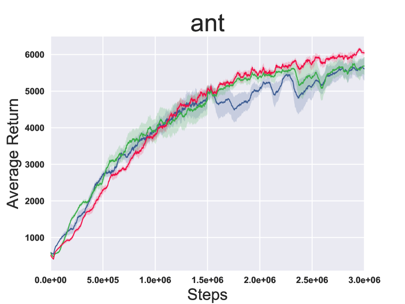
Refer to caption
Refer to caption
Refer to caption
Figure 7: Training curves on additional continuous control benchmarks Mujoco-v1.

I.3 Additional MuJoCo-v2 Experiments
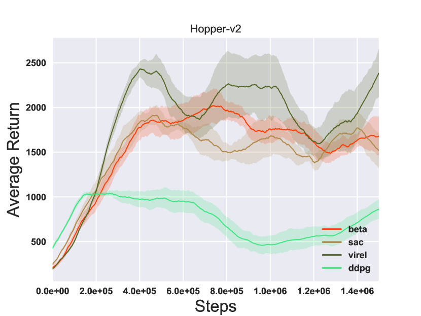
Refer to caption
Refer to caption
Refer to caption
Refer to caption
Refer to caption
Refer to caption
Figure 8: Training curves on additional continuous control benchmarks gym-Mujoco-v2.