Cylindric rhombic tableaux and the two-species ASEP on a ring

Abstract.

The asymmetric simple exclusion process (ASEP) is a model of particles hopping on a one-dimensional lattice of $n$ sites. It was introduced around 1970 [MGP68, Spi70], and since then has been extensively studied by researchers in statistical mechanics, probability, and combinatorics. Recently the ASEP on a lattice with open boundaries has been linked to Koornwinder polynomials [CW15, Can17], and the ASEP on a ring has been linked to Macdonald polynomials [CdGW15]. In this article we study the two-species asymmetric simple exclusion process (ASEP) on a ring, in which two kinds of particles (“heavy” and “light”), as well as “holes,” can hop both clockwise and counterclockwise (at rates $1$ or $t$ depending on the particle types) on a ring of $n$ sites. We introduce some new tableaux on a cylinder called cylindric rhombic tableaux (CRT), and use them to give a formula for the stationary distribution of the two-species ASEP – each probability is expressed as a sum over all CRT of a fixed type. When $\lambda$ is a partition in $\{0,1,2\}^{n}$, we then give a formula for the nonsymmetric Macdonald polynomial $E_{\lambda}$ and the symmetric Macdonald polynomial $P_{\lambda}$ by refining our tableaux formulas for the stationary distribution.

1. Introduction

Introduced around 1970 [MGP68, Spi70], the asymmetric simple exclusion process (ASEP) is a model of interacting particles hopping on a one-dimensional lattice of $n$ sites. It has been extensively studied by researchers in statistical mechanics [DEHP93, USW04], probability [Lig05, Lig75, FM07, BC14], and combinatorics [DS05, Ang06, BE04, CW07, CW11, CMW17]. Recently the ASEP on a lattice with open boundaries has been linked to Koornwinder polynomials [CW15, Can17], and the ASEP on a ring has been linked to Macdonald polynomials [CdGW15]. In particular, it was shown in [CdGW15] that when $q=1$ and $x_{i}=1$ for all $i$, the Macdonald polynomial $P_{\lambda}$ is the partition function for the multispecies ASEP on a ring.

In this article we study the two-species asymmetric simple exclusion process (ASEP) on a ring, in which two kinds of particles (“heavy” and “light”) hop on a lattice of $n$ sites arranged in a ring. Two adjacent particles, or a particle and a hole, can switch places at a rate $t$ or $1$, depending on their relative weights. We introduce some new tableaux on a cylinder called cylindric rhombic tableaux (CRT), and use them to give a formula for the stationary distribution of the ASEP – each probability is expressed as a sum over the weights of all CRT of a fixed type, where the weight of each CRT is a series. When $\lambda$ is a partition in $\{0,1,2\}^{n}$, we then give a formula for the nonsymmetric Macdonald polynomial $E_{\lambda}$ and the symmetric Macdonald polynomial $P_{\lambda}$ by refining our tableaux formulas for the stationary distribution.

When $t=0$, the asymmetric simple exclusion process is called the totally asymmetric simple exclusion process or TASEP. Ferrari and Martin [FM07] studied the multispecies ($k$-species) TASEP on a ring and gave combinatorial formulas for the stationary distribution in terms of multiline queues; they viewed the $k$-TASEP on a ring as a projection of a Markov process on multiline queues, which can be viewed as a coupled system of $k$ single species TASEPs. This work was recently generalized by Martin [Mar18] to the case of ASEP (i.e. $t$ is general). Matrix product formulas were found for the probabilities of the TASEP using probabilistic methods in [EFM09] and generalized to the ASEP case in [PEM09a] with an explicit construction in [AAMP12]. From the statistical mechanics side, other formulas for the $k$-TASEP were found by interpreting the Ferrari-Martin process as a combinatorial $R$ matrix in [KMO15]. The inhomogeneous multispecies TASEP was also studied in [AL14], with a graphical construction that generalized the Ferrari-Martin algorithm for the 2-TASEP, and a general conjecture for the $k$-TASEP which was proved using a generalized Matrix ansatz in [AM13].

Multiline queues have been used to study many aspects of the ASEP [AL14, AL18]; in this case we give a bijection between CRT and multiline queues, which is related to recent work by the second author [Man17]. Also note that Haglund-Haiman-Loehr have a tableaux formula for both symmetric [HHL05a] and nonsymmetric Macdonald polynomials [HHL05b] using nonattacking fillings; we explain the relation between nonattacking fillings and multiline queues in [CMW18] (they are in bijection when the partition has distinct parts; but in general there are more nonattacking fillings than multiline queues).

Remark 1.1.

In some sense the results of this paper are subsumed by the results of [CMW18], in that the latter has combinatorial formulas that work for Macdonald polynomials associated to arbitrary partitions (not just $\lambda\in\{0,1,2\}^{n}$). However, since these cylindric rhombic tableaux are significantly different than multiline queues, and our methods of proof use the Matrix Ansatz rather than the Hecke algebra, we thought that this paper might be of independent interest.

2. The ASEP on a ring

We now define the two-species asymmetric simple exclusion process (ASEP) on a ring.

Definition 2.1.

Let $k$, $r$, and $\ell$ be nonnegative integers which sum to $n$, and let $t$ be a constant such that $0\leq t\leq 1$. Let $\operatorname{States}(k,r,\ell)$ be the set of all words of length $n$ in $\{0,1,2\}^{n}$ consisting of $k$ $0$’s, $r$ $1$’s, and $\ell$ $2$’s. We consider indices modulo $n$; i.e. if $\mu=\mu_{1}\ldots\mu_{n}\in\{0,1,2\}^{n}$, then $\mu_{n+1}=\mu_{1}$. The two-species asymmetric simple exclusion process $\operatorname{ASEP}ASEP(k,r,\ell)$ on a ring is the Markov chain on $\operatorname{States}(k,r,\ell)$ with transition probabilities $P_{\mu,\nu}$ between states $\mu,\nu\in\operatorname{States}(k,r,\ell)$:

• If $\mu=AijB$ and $\nu=AjiB$, where $A$ and $B$ are words in $\{0,1,2\}^{*}$ and $i>j$ are letters in $\{0,1,2\}$, then $P_{\mu,\nu}=\frac{t}{n}$ and $P_{\nu,\mu}=\frac{1}{n}$.

• Otherwise, $P_{\mu,\nu}=0$ for $\nu\neq\mu$ and $P_{\mu,\mu}=1-\sum_{\mu\neq\nu}P_{\mu,\nu}$.

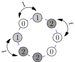
Figure 1. The two-species ASEP on a lattice with $8$ sites. There are three holes ($0$’s), two light particles ($1$’s), and three heavy particles ($2$’s), so we refer to this Markov chain as $\operatorname{ASEP}ASEP(3,2,3)$.

We think of the $1$’s and $2$’s as representing two types of particles (“light” and “heavy”) which can occupy the sites; each $0$ denotes an empty site.

The following Matrix Ansatz [DJLS93] (see also [PEM09b]) is a useful tool for computing these probabilities in terms of the trace of a certain matrix product.

Theorem 2.2 (Matrix Ansatz).

[DJLS93, Section 8] Suppose that $A_{0}$, $A_{1}$, and $A_{2}$ are matrices (typically infinite) that satisfy the following relations:

(1) $$A_{0}A_{2}=tA_{2}A_{0}+(1-t)(A_{0}+A_{2}),\qquad A_{0}A_{1}=tA_{1}A_{0}+(1-t)A_{1},\qquad A_{1}A_{2}=tA_{2}A_{1}+(1-t)A_{1}.$$

Given $\mu\in\operatorname{States}(k,r,\ell)$, we let $\operatorname{Mat}(\mu)$ denote the product of matrices obtained from $\mu$ by substituting $A_{0}$ for $0$, $A_{1}$ for $1$, and $A_{2}$ for $2$. Then in the $\operatorname{ASEP}ASEP(k,r,\ell)$, the steady state probability $\Pr(\mu)$ of state $\mu$ is given by

$$\Pr(\mu)=\frac{1}{Z_{k,r,\ell}}\operatorname{tr}(\operatorname{Mat}(\mu)),$$

where $Z_{k,r,\ell}$ is the partition function defined by $[x^{k}y^{r}z^{\ell}]\operatorname{tr}((xA_{0}+yA_{1}+zA_{2})^{k+r+\ell})$.

3. Probabilities for the two-species ASEP using cylindric rhombic tableaux

In this section we define some new combinatorial objects that we call cylindric rhombic tableaux (or CRT), and then in 3.17 we use them to give combinatorial formulas for the steady state probabilities of the ASEP. The proof of our formulas uses the Matrix Ansatz. Our combinatorial objects will be fillings of certain diagrams composed of squares and rhombi. The squares have two horizontal and two vertical edges, while the rhombi have two vertical edges as well as two diagonal edges (of slope $1)$, see Figure 2. The fact that states of the $\operatorname{ASEP}ASEP$ are words in $\{0,1,2\}^{*}$ is related to the fact that there are three types of lines making up the sides of a square or rhombus: vertical, diagonal, and horizontal.

Definition 3.1.

A (generalized) row in a CRT is a connected strip of squares and rhombi which are adjacent along their vertical edges, see the left diagram in Figure 2. A square column is a connected strip of squares, which are adjacent along their horizontal edges; and a rhombic column is a connected strip of rhombi, which are adjacent along their diagonal edges.

Definition 3.2.

Given $\mu\in\{0,1,2\}^{*}$, we define $\mu|_{12}$ to be the subword of $\mu$ consisting of 1’s and 2’s. An $\mu$-strip is a generalized row composed of adjacent squares and rhombi which is obtained by reading $\mu|_{12}$ and appending a square for each 2 and a rhombus for each 1 to the left of the row; see the left diagram in Figure 2.

Definition 3.3.

Given $\mu\in\{0,1,2\}^{*}$, we define the $\mu$-path $P(\mu)$ to be the lattice path consisting of south, southwest, and west steps obtained by reading $\mu$ and mapping a 0 to a south step, a 1 to a southwest step, and a 2 to a west step; see the bold path at the right of Figure 2.

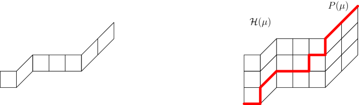
Figure 2. For $\mu=1102022102$, the $\mu$-strip is shown at the left, while $\mathcal{H}(\mu)$ is shown at the right, with the path $P(\mu)$ superimposed in bold.

Definition 3.4.

Let $\mu\in\operatorname{States}(k,r,\ell)$. Define the $\mu$-diagram $\mathcal{H}(\mu)$ to be the shape consisting of $k$ $\mu$-strips stacked on top of each other, together with the path $P(\mu)$ superimposed onto the shape so that it connects the northeast and southwest corners. (If $k=0$ then $\mathcal{H}(\mu)$ is defined to be just the path $P(\mu)$.) See the diagram at the right in Figure 2. We identify the two vertical edges on either end of each row; in this way we view the shape on a cylinder. Thus the rightmost tile is adjacent to the leftmost tile in each row.

Note that for $\mu\in\operatorname{States}(k,r,\ell)$, $\mathcal{H}(\mu)$ has $k$ rows, $r$ rhombic columns, and $\ell$ square columns. For example in Figure 2, $\mathcal{H}(\mu)$ has $3$ rows, $3$ rhombic columns, and $4$ square columns. For $m\in[k]$, let $\operatorname{row}(m)$ denote the $m$’th row, numbered from bottom to top.

Definition 3.5 (Cylindric rhombic tableau and arrow ordering).

Choose a word $\mu\in\operatorname{States}(k,r,\ell)$. A cylindric rhombic tableau (CRT) $T$ of type $\mu$ is a placement of up-arrows into the square tiles of the diagram $\mathcal{H}(\mu)$ so that there is at most one up-arrow in each column. (We allow columns to be empty.) We denote the set of cylindric rhombic tableaux of type $\mu$ by $\operatorname{CRT}(\mu)$.

An arrow ordering of $T$ is a labeling of the arrows in each row by the numbers $1,\dots,i$, where $i$ is the number of arrows in that row. Let $\operatorname{arr}(T)$ denote the total number of arrows in $T$. We let $\sigma^{i}$ denote the labeling of the arrows in $\operatorname{row}(i)$, and let $\{\sigma^{i}\}=(\sigma^{1},\dots,\sigma^{k})$.

For an example, see Figure 3.

Definition 3.6.

We say an arrow in tile $s$ is pointing at a tile $s^{\prime}$ if they are in the same column and $s$ is below $s^{\prime}$ when we read from bottom to top. We call a square tile free if the tile is empty and there is no arrow pointing to it. (Note that freeness does not depend on the path $P(\mu)$.)

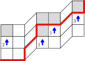
Figure 3. A cylindric rhombic tableau $T$ of type $0212201022$ with a chosen arrow ordering $\sigma$. The square tiles that are not free are grey.

We will define the weight of each cylindric rhombic tableau. To do so, we need to introduce a few combinatorial statistics.

Definition 3.7.

Given a subset $I$ of a finite sequence $U$ where $|U|=m$, we let $\operatorname{Sym}_{I,U}$ denote the set of total orders on $I$, which we also call partial permutations. We write the elements of $\operatorname{Sym}_{I,U}$ as strings of length $m$, with a $*$ denoting elements not in $I$.

For example, if $U=\{1,2,\dots,6\}$ and $I=\{1,2,4\}$, then there are $|I|!$ total orders on $I$, which we denote by

$$\operatorname{Sym}_{I,U}=\{1\ 2\ *\ 3\ *\ *,\ 1\ 3\ *\ 2\ *\ *,\ 2\ 1\ *\ 3\ *\ *,\ 2\ 3\ *\ 1\ *\ *,\ 3\ 1\ *\ 2\ *\ *,\ 3\ 2\ *\ 1\ *\ *\}.$$

Definition 3.8 (Disorder).

Let $\widetilde{\operatorname{Sym}}_{I,U}$ denote the set of all sequences that can be obtained from the elements of $\operatorname{Sym}_{I,U}$ be inserting a $0$ in an arbitrary position. Given $\tilde{\sigma}\in\widetilde{\operatorname{Sym}}_{I,U}$, we define its disorder $\operatorname{dis}(\tilde{\sigma})$ inductively as follows:

Reading the entries of $\tilde{\sigma}$ from left to right starting from the $0$, we let $\operatorname{dis}_{1}(\tilde{\sigma})$ equal the number of $*$’s or numbers bigger than $1$ we encounter before we reach the $1$. We then let $\operatorname{dis}_{2}(\tilde{\sigma})$ be the number of $*$’s or numbers bigger than $2$ we encounter if we travel from the $1$ to the $2$ from left to right, wrapping around to the beginning of $\tilde{\sigma}$ if necessary. Similarly, $\operatorname{dis}_{i}(\tilde{\sigma})$ is the number of $*$’s or numbers bigger than $i$ we encounter if we travel from the $i-1$ to the $i$ from left to right, wrapping around if necessary. Finally we define the disorder to be $\operatorname{dis}(\tilde{\sigma})=\operatorname{dis}_{1}(\tilde{\sigma})+\operatorname{dis}_{2}(\tilde{\sigma})+\dots+\operatorname{dis}_{|I|}(\tilde{\sigma}).$

If $\tilde{\sigma}=0\ 2\ 1\ *\ 3\ *\ *$, then $\operatorname{dis}_{1}(\tilde{\sigma})=1$, $\operatorname{dis}_{2}(\tilde{\sigma})=4$, $\operatorname{dis}_{3}(\tilde{\sigma})=1$, and $\operatorname{dis}(\tilde{\sigma})=6$.

Remark 3.9.

In a recent paper [KM17], a statistic very similar to disorder, called betrayal, was introduced on certain colored words in a formula for modified symmetric Macdonald polynomials $\tilde{H}_{\lambda}$. It would be interesting to understand the connection between the statistics on these different objects.

Definition 3.10 (From an arrow ordering to a partial permutation).

Given a cylindric rhombic tableau $T$ and an arrow ordering $\{\sigma^{i}\}$, we associate a partial permutation to each row of $T$ as follows. We fix $\operatorname{row}(i)$ and read its elements from right to left, skipping over non-free square tiles, but recording free square tiles and rhombic tiles by a $*$, and arrows by their label. We also record the vertical line in $P(\mu)$ by a $0$. We denote this partial permutation by $\tilde{\sigma}^{i}$.

For example, the rows of the tableau in Figure 3 would give rise to the sequences $\tilde{\sigma}^{1}=*\ *\ *\ 1\ *\ 0\ *\ *$, $\tilde{\sigma}^{2}=3\ *\ 1\ 0\ *\ *\ 2$, and $\tilde{\sigma}^{3}=0\ *\ *\ *$ (which are read from left to right).

We now define the disorder for arrow orderings of cylindric rhombic tableaux.

Definition 3.11 (Disorder of a CRT with an arrow ordering).

Given a cylindric rhombic tableau $T$ with $k$ rows and an arrow ordering $\{\sigma^{i}\}=\{\sigma^{1},\ldots,\sigma^{k}\}$, we define the disorder of $(T,\{\sigma^{i}\})$ to be

$$\operatorname{dis}(T,\{\sigma^{i}\})=\sum_{i=1}^{k}\operatorname{dis}(\tilde{\sigma}^{i}).$$

Example 3.12.

Using $(T,\{\sigma^{i}\})$ from Figure 3, we compute $\operatorname{dis}(*\ *\ *\ 1\ *\ 0\ *\ *)=5$, $\operatorname{dis}(3\ *\ 1\ 0\ *\ *\ 2)=5+2+0=7$, and $\operatorname{dis}(0\ *\ *\ *)=0$, so $\operatorname{dis}(T,\{\sigma^{i}\})=12$.

We let $[i]=[i]_{t}$ denote the $t$-analogue of the positive integer $i$, that is, $[i]=\frac{1-t^{i}}{1-t}=1+t+\ldots+t^{i-1}$. We also let $[i]!=[1][2]\ldots[i]$.

Definition 3.13.

The $t$-weight $\operatorname{wt}_{t}(T)$ of a cylindric rhombic tableau $T$ of type $\mu\in\operatorname{States}(k,r,\ell)$ is computed as follows.

Given an arrow ordering $\{\sigma^{i}\}$ of the arrows in $T$, we define

$$\operatorname{wt}_{t}(T,\{\sigma^{i}\})=t^{\operatorname{dis}(T,\{\sigma^{i}\})}.$$

We then define the $t$-weight of $T$ to be

$$\operatorname{wt}_{t}(T)=\frac{[r+\ell-\operatorname{arr}(T)]!}{[r+\ell]!}\sum_{\{\sigma^{i}\}}\operatorname{wt}_{t}(T,\{\sigma^{i}\}),$$

where $\{\sigma^{i}\}$ varies over all possible arrow orderings of $T$.

Example 3.14.

Continuing Example 3.12, with Figure 3, we have $r=2$, $\ell=5$, and $\operatorname{arr}(T)=4$. Thus $\frac{[r+\ell-\operatorname{arr}(T)]!}{[r+\ell]!}=\frac{1}{[7][6][5][4]}$.

To compute $\operatorname{wt}_{t}(T)$, we need to consider all possible arrow orderings. Note that:

• There is only one arrow ordering of $\operatorname{row}(1)$ and of $\operatorname{row}(3)$, so the weight contributed to $\operatorname{wt}_{t}(T)$ by the possible arrow orderings of $\operatorname{row}(1)$ and $\operatorname{row}(3)$ is just $t^{5}$.

• If we represent the arrows versus rhombic/free tiles in $\operatorname{row}(2)$ by $x$’s and $*$’s, respectively, then the content of $\operatorname{row}(2)$ can be encoded by the sequence $x\ *\ x\ 0\ *\ *\ x$. We have $\operatorname{dis}(1\ *\ 2\ 0\ *\ *\ 3)=6$, $\operatorname{dis}(1\ *\ 3\ 0\ *\ *\ 2)=8$, $\operatorname{dis}(2\ *\ 1\ 0\ *\ *\ 3)=11$, $\operatorname{dis}(2\ *\ 3\ 0\ *\ *\ 1)=3$, $\operatorname{dis}(3\ *\ 1\ 0\ *\ *\ 2)=7$, and $\operatorname{dis}(3\ *\ 2\ 0\ *\ *\ 1)=6$. Thus the weight contributed by the possible arrow labelings of $\operatorname{row}(2)$ (only one of which is shown in Figure 3) of is $t^{3}+2t^{6}+t^{7}+t^{8}+t^{11}$.

Letting $I_{i}$ denote the positions of the arrows in $\operatorname{row}(i)$ and $U_{i}$ denote the positions of the arrows and free tiles in $\operatorname{row}(i)$, we can write the total weight of this tableau for all possible arrow orderings $\{\sigma^{i}\}=(\sigma^{1},\dots,\sigma^{5})$ as

$$\operatorname{wt}_{t}(T)=\frac{1}{[7][6][5][4]}\prod_{m=1}^{3}\sum_{\sigma^{m}\in\operatorname{Sym}_{I_{m},U_{m}}}t^{\operatorname{dis}(\tilde{\sigma}^{m})}=\frac{(t^{5})(t^{3}+2t^{6}+t^{7}+t^{8}+t^{11})}{[7][6][5][4]}.$$

Remark 3.15.

It is interesting to note that if $I=U$, disorder on $\operatorname{Sym}_{I,U}=\operatorname{Sym}_{|I|}$ is a Mahonian statistic, i.e. it has the same distribution as inversions.

Definition 3.16 (Combinatorial partition function).

Given $\mu\in\operatorname{States}(k,r,\ell)$, we define

$$\operatorname{Tab}_{t}(\mu):=\sum_{T\in\operatorname{CRT}(\mu)}\operatorname{wt}_{t}(T).$$

We also define the combinatorial partition function of the cylindric rhombic tableaux to be

$$\mathcal{Z}_{k,r,\ell}(t)=\sum_{\mu\in\operatorname{States}(k,r,\ell)}\operatorname{Tab}_{t}(\mu).$$

We are finally ready to state the first main result of this paper.

Theorem 3.17.

Consider the two-species asymmetric simple exclusion process $\operatorname{ASEP}ASEP(k,r,\ell)$. Then the steady state probability of being in state $\mu$, where $\mu\in\operatorname{States}(k,r,\ell)$, is

$$\Pr(\mu)=\frac{\operatorname{Tab}_{t}(\mu)}{\mathcal{Z}_{k,r,\ell}(t)},$$

where $\operatorname{Tab}_{t}(\mu)$ and $\mathcal{Z}_{k,r,\ell}(t)$ are as in 3.16.

Example 3.18.

To compute the steady state probability $\Pr(221100)$ of the state $221100$ of the $\operatorname{ASEP}ASEP(2,2,2)$, we need to sum the weights of all cylindric rhombic tableaux of type $221100$, see Figure 4. We then find that $\Pr(221100)=\frac{(t+1)(t^{4}+t^{3}+6t^{2}+t+6)}{[4][3]Z_{2,2,2}}.$

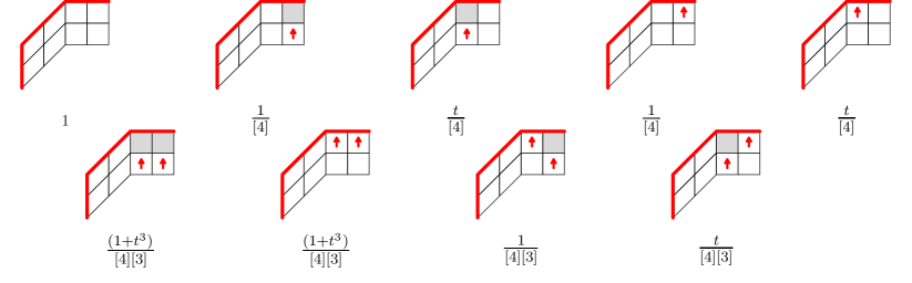
Figure 4. The cylindric rhombic tableaux of type $221100$ and their weights.

Example 3.19.

To compute the steady state probability $\Pr(201021)$ of the state $201021$ of the $\operatorname{ASEP}ASEP(2,2,2)$, we need to sum the weights of all cylindric rhombic tableaux of type $201021$, see Figure 5. We then find that $\Pr(201021)=\frac{(t+1)(t^{2}+t+1)(2t^{2}+t+2)}{[4][3]\mathcal{Z}_{2,2,2}(t)}.$

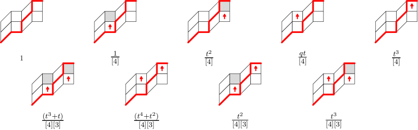
Figure 5. The cylindric rhombic tableaux of type $201021$ and their weights.

Remark 3.20.

For a given state $\mu$ of the $\operatorname{ASEP}ASEP(k,r,\ell)$, we can multiply $\operatorname{Tab}_{t}(\mu)$ by the scalar $[r+\ell]!/[r]!$ to obtain polynomials in $t$ with positive coefficients. The resulting polynomials display a “particle-hole symmetry,” see 6.11 and 6.12.

4. Formulas for Macdonald polynomials using cylindric rhombic tableaux

Symmetric Macdonald polynomials [Mac95] are a family of multivariable orthogonal polynomials indexed by partitions, whose coefficients depend on two parameters $q$ and $t$. In recent works [CdGW15, CdGW], Cantini, de Gier, and Wheeler gave a link between the multi-species exclusion process on a ring and Macdonald polynomials. In this section we will give a combinatorial formula for Macdonald polynomials in a special case; the proof of our formula uses some results from [CdGW15].

Let $F=\mathbb{Q}(q,t)$ be the field of rational functions in $q$ and $t$, and let $m_{\lambda}$ denote the monomial symmetric polynomial indexed by the partition $\lambda$. The Macdonald polynomials are defined as follows.

Definition 4.1.

Let $\langle\cdot,\cdot\rangle$ denote the Macdonald inner product on power sum symmetric functions [Mac95, Chapter VI, Equation (1.5)], where $<$ denotes the dominance order on partitions [Mac95, Chapter I, Section 1]. The Macdonald polynomial $P_{\lambda}(x_{1},\dots,x_{n};q,t)$ is the unique homogeneous symmetric polynomial in $x_{1},\dots,x_{n}$ with coefficients in $F$ which satisfies

$$\langle P_{\lambda},P_{\mu}\rangle =0,\text{ for }\lambda\neq\mu,$$

$$P_{\lambda}(x_{1},\dots,x_{n};q,t) =m_{\lambda}(x_{1},\dots,x_{n})+\sum_{\mu<\lambda}c_{\lambda,\mu}(q,t)m_{\mu}(x_{1},\dots,x_{n}),$$

i.e. the coefficients $c_{\lambda,\mu}(q,t)$ of the lower degree terms are determined by the orthogonality conditions.

The nonsymmetric Macdonald polynomials $E_{\mu}$, which are indexed by compositions, were later defined by Opdam [Opd95] and Cherednik [Che95b, Che95a] as joint eigenfunctions of a family of commuting operators in the double affine Hecke algebra, with $P_{\lambda}$ obtained as a sum over the $E_{\mu}$:

$$P_{\lambda}=\sum_{\mu}E_{\mu},$$

for $\mu$ ranging over all permutations of $\lambda$. For more details, see [Mac95].

In this section we enhance our weight function on tableaux, to include an additional parameter $q$ and variables $x_{1},\dots,x_{n}$ (where $n=k+r+\ell$). We then give our second main result, which is a formula for certain Macdonald polynomials in terms of cylindric rhombic tableaux. In particular, we will give a formula for the nonsymmetric Macdonald polynomial $E_{\lambda}$ and a formula for the symmetric Macdonald polynomial $P_{\lambda}$, where $\lambda$ is any partition in $\{0,1,2\}^{*}$. Note that Haglund, Haiman and Loehr have given combinatorial formulas for both the nonsymmetric Macdonald polynomials and the symmetric Macdonald polynomials in terms of nonattacking fillings of composition diagrams [HHL05a, HHL05b]; it would be interesting to understand how our formulas relate to theirs.

Definition 4.2.

We refer to the left and right border of a cylindric tableau (which are identified) as its vertical boundary. Given a cylindric rhombic tableau $T$ with path $P(\mu)$ and arrow ordering $\{\sigma^{i}\}$, for each row $\operatorname{row}(i)$, we define $\operatorname{cyc}(T,\sigma^{i})$ to be the number of times we cross the vertical boundary if we start at the vertical line in $P(\mu)$ in row $i$ and then travel from right to left (wrapping around if necessary) to the arrow labeled $1$, then the arrow labeled $2$, and so on. We define the cycling of $(T,\{\sigma^{i}\})$ to be

$$\operatorname{cyc}(T,\{\sigma^{i}\})=\sum_{i}\operatorname{cyc}(T,\sigma^{i}).$$

Recall that a recoil of a (partial) permutation $\sigma$ is a pair $(j+1,j)$ such that $\sigma^{-1}(j+1)<\sigma^{-1}(j)$. In other words, it is a pair of values $(j+1,j)$ where $j+1$ appears to the left of $j$ in $\sigma$. For example, the partial permutation $3*10**2$ has two recoils, $(1,0)$ and $(3,2)$. Note that $\operatorname{cyc}(T,\sigma)$ for a given row’s arrow ordering $\{\sigma^{i}\}$ is equal to the number of recoils of $\tilde{\sigma}$ (see 3.10). The cycling statistic defined above will contribute to the power of $q$ associated to each tableau and arrow ordering.

Now given a CRT with path $P(\mu)$, let us number the steps of $P(\mu)$ from northeast to southwest using the numbers $1,2,\dots,n$, where $n=|\mu|$; see Figure 6. This allows us to give every row and column of $\mathcal{H}(\mu)$ a unique integer label, and we will subsequently refer to row $i$ and column $j$ using this labeling.

Figure 6. A cylindric rhombic tableau of type $\mu=0212201022$, with the steps of $P(\mu)$ labeled from $1$ to $10$.

Definition 4.3.

The $x$-weight $\operatorname{wt}_{x}(T,\{\sigma^{i}\})$ of a cylindric rhombic tableau $T$ of type $\mu\in\operatorname{States}(k,r,\ell)$ with an arrow ordering $\{\sigma^{i}\}$ is computed as follows.

For each arrow $a$ in $T$, if its label given by the arrow ordering is the maximum among all arrows in its row, then we set $\operatorname{wt}(a)=x_{i}$, where $i$ is the row label of the square containing $a$. Otherwise, we set $\operatorname{wt}(a)=x_{j}$, where $j$ is the column label of the square containing $a$.

For each column $c$ of squares in $T$, if $c$ contains no arrows, we set $\operatorname{wt}(c)=x_{j}$, where $j$ is the column label of $c$. Otherwise we set $\operatorname{wt}(c)=1$.

We also define $\operatorname{wt}_{12}(\mu):=\prod_{k\in\operatorname{\operatorname{Pos}_{12}}(\mu)}x_{k}$, where $\operatorname{\operatorname{Pos}_{12}}(\mu)=\{i\ |\ \mu_{i}=1\text{ or }2\}$.

Finally we define the $x$-weight $\operatorname{wt}_{x}(T,\{\sigma^{i}\})$ of $(T,\{\sigma^{i}\})$ to be

$$\operatorname{wt}_{x}(T,\{\sigma^{i}\})=\operatorname{wt}_{\operatorname{\operatorname{Pos}_{12}}}(\mu)\prod_{a}\operatorname{wt}(a)\prod_{c}\operatorname{wt}(c),$$

where the products are over all arrows $a$ and columns $c$ of squares of $T$.

Remark 4.4.

It follows from the above definition that given a CRT $T$ of type $\mu\in\operatorname{States}(k,r,\ell)$, the $x$-weight of $T$ is a monomial in $x_{1}\dots x_{n}$ of degree $r+2\ell$.

Example 4.5.

Figure 6 shows a cylindric rhombic tableau $T$ of type $0212201022$ together with an arrow ordering $\{\sigma^{i}\}$. In this example we have $\prod_{a}\operatorname{wt}(a)=x_{4}x_{6}x_{8}x_{10}$, $\prod_{c}\operatorname{wt}(c)=x_{9}$, $\operatorname{wt}_{\operatorname{\operatorname{Pos}_{12}}}(\mu)=x_{2}x_{3}x_{4}x_{5}x_{7}x_{9}x_{10}$. Therefore

$$\operatorname{wt}_{x}(T,\{\sigma^{i}\})=x_{2}x_{3}x_{4}^{2}x_{5}x_{6}x_{7}x_{8}x_{9}^{2}x_{10}^{2}.$$

Given a positive integer $i$, let $[i]_{qt}=\frac{1-qt^{i}}{1-t}$, and let $[i]_{qt}!=[i]_{qt}[i-1]_{qt}\dots[1]_{qt}$. Note that when $q=1$, $[i]_{qt}$ recovers the quantity $[i]=[i]_{t}$ we defined earlier. Finally we are ready to define the $qtx$-weight of a cylindric rhombic tableau.

Definition 4.6.

Let $T$ be a cylindric rhombic tableau of type $\mu\in\operatorname{States}(k,r,\ell)$, and and let $\{\sigma^{i}\}$ be an arrow ordering of its arrows. The $qtx$-weight $\operatorname{wt}_{qtx}(T,\{\sigma^{i}\})$ is defined to be

(2) $$\operatorname{wt}_{qtx}(T,\{\sigma^{i}\})={t^{\operatorname{dis}(T,\{\sigma^{i}\})}q^{\operatorname{cyc}(T,\{\sigma^{i}\})}\operatorname{wt}_{x}(T,\{\sigma^{i}\})}.$$

We then define the $qtx$-weight of $T$ to be

$$\operatorname{wt}_{qtx}(T)=\frac{[r+\ell-\operatorname{arr}(T)]_{qt}!}{[r+\ell]_{qt}!}\sum_{\{\sigma^{i}\}}\operatorname{wt}_{qtx}(T,\{\sigma^{i}\}),$$

where $\{\sigma^{i}\}$ varies over all possible arrow orderings of $T$.

Definition 4.7.

Given $\mu\in\operatorname{States}(k,r,\ell)$, we define

$$\operatorname{Tab}_{qtx}(\mu):=\sum_{T\in\operatorname{CRT}(\mu)}\operatorname{wt}_{qtx}(T)$$

Example 4.8.

Figure 7 shows the cylindric rhombic tableaux of type $201021$. The sum of the weights of all the tableaux is $\operatorname{Tab}_{qtx}(201021)=x_{1}^{2}x_{3}x_{5}^{2}x_{6}+\frac{(x_{1}+qt^{2}x_{5})x_{1}x_{3}x_{4}x_{5}x_{6}}{[4]_{qt}}+\frac{(tx_{1}+qt^{3}x_{5})x_{1}x_{2}x_{3}x_{5}x_{6}}{[4]_{qt}}+\frac{q(t^{3}x_{1}+tx_{5})x_{1}x_{3}x_{4}x_{5}x_{6}}{[4]_{qt}[3]_{qt}}+\frac{q(t^{4}x_{1}+t^{2}x_{5})x_{1}x_{2}x_{3}x_{5}x_{6}}{[4]_{qt}[3]_{qt}}+\frac{q(t^{2}+t^{3})x_{1}x_{2}x_{3}x_{4}x_{5}x_{6}}{[4]_{qt}[3]_{qt}}$.

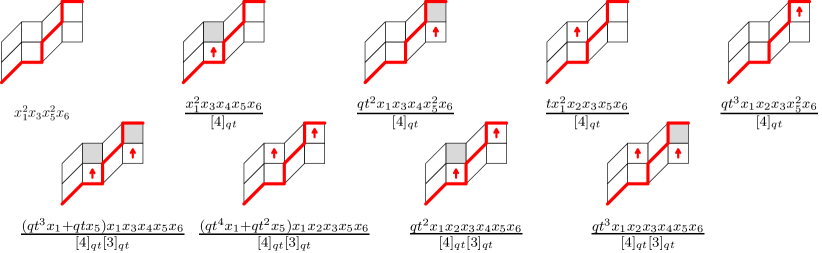
Figure 7. All cylindric rhombic tableaux of type $201021$, along with their weights.

The second main result of this paper is the following.

Theorem 4.9.

For any partition $\lambda=(\lambda_{1},\dots,\lambda_{n})$ of the form $2^{\ell}1^{r}0^{k}$, we have that the nonsymmetric Macdonald polynomial $E_{\lambda}$ is given by

(3) $$E_{\lambda}(x_{1},\dots,x_{n};q,t)=\operatorname{Tab}_{qtx}(2^{\ell}1^{r}0^{k}).$$

Moreover the symmetric Macdonald polynomial $\mathcal{P}_{\lambda}$ is given by

(4) $$\mathcal{P}_{\lambda}(x_{1},\dots,x_{n};q,t)=\sum_{\mu}\operatorname{Tab}_{qtx}(\mu),$$

where the sum runs through all distinct permutations $\mu$ of $\lambda$.

Example 4.10.

Using SageMath [The18], we find that the nonsymmetric Macdonald polynomial $E_{221100}=E_{221100}(x_{1},\dots,x_{6};q,t)$ equals

$$E_{221100}=x_{1}^{2}x_{2}^{2}x_{3}x_{4}+\frac{q(x_{1}+x_{2})(x_{5}+x_{6})x_{1}x_{2}x_{3}x_{4}}{[3]_{qt}}+\frac{q^{2}(1+t)x_{1}x_{2}x_{3}x_{4}x_{5}x_{6}}{[3]_{qt}[4]_{qt}}.$$

This agrees with the sum of the weights of the tableaux of type $\mu=221100$, see Figure 8.

Figure 8. All cylindric rhombic tableaux of type $221100$, along with their weights.

5. The Matrix Ansatz and the results of Cantini-deGier-Wheeler

In order to prove 3.17 and 4.9, we need to introduce some matrices from [CdGW15], which can be used to compute certain Macdonald polynomials.

Definition 5.1.

[CdGW15, (53)] We define semi-infinite matrices $A_{0}(x)$, $A_{1}(x)$, $A_{2}(x)$, and $S$, whose rows and columns are indexed by $\mathbb{Z}_{\geq 0}$.

Let $A_{0}(x)=(A_{0}(x)_{i,j})$ be defined by

$$A_{0}(x)_{i,j}=\left\{\begin{array}[]{ll}1&{\rm if}\ i=j\\ x&{\rm if}\ i=j-1\\ 0&{\rm otherwise}.\end{array}\right.$$

Let $A_{2}(x)=(A_{2}(x)_{i,j})$ be defined by

$$A_{2}(x)_{i,j}=\left\{\begin{array}[]{ll}x^{2}&{\rm if}\ i=j\\ x(1-t^{i})&{\rm if}\ i=j+1\\ 0&{\rm otherwise.}\end{array}\right.$$

Let $A_{1}(x)=(A_{1}(x)_{i,j})$ be a diagonal matrix defined by

$$A_{1}(x)_{i,i}=xt^{i}.$$

Let $S=(S_{i,j})$ be a diagonal matrix defined by

$$S_{i,i}=q^{i}.$$

Cantini, deGier, and Wheeler [CdGW15] proved that Macdonald polynomials can be computed in terms of the matrices above as follows. (We restrict to the setting where compositions have parts equal to $0$, $1$, or $2$.)

Theorem 5.2.

[CdGW15, (16),(24), Lemma 3] Given a composition $\mu=(\mu_{1},\dots,\mu_{n})\in\{0,1,2\}^{n}$, let $\lambda$ be the partition obtained from $\mu$ by sorting its parts, and set

(5) $$\Omega_{\lambda}(q,t)=\prod_{1\leq i<j\leq s}({1-q^{j-i}t^{\lambda^{\prime}_{i}-\lambda^{\prime}_{j}}}),$$

where $s$ is the largest part of $\lambda$. We define

(6) $$f_{\mu}(x_{1},\dots,x_{n};q,t)=\Omega_{\lambda}\operatorname{tr}[A_{\mu_{1}}(x_{1})\dots A_{\mu_{n}}(x_{n})S].$$

For any partition $\lambda=(\lambda_{1},\dots,\lambda_{n})\in\{0,1,2\}^{*}$, the nonsymmetric Macdonald polynomial $E_{\lambda}$ is given by

(7) $$E_{\lambda}(x_{1},\dots,x_{n};q,t)=f_{\lambda}(x_{1},\dots,x_{n};q,t).$$

Moreover the symmetric Macdonald polynomial $\mathcal{P}_{\lambda}$ is given by

(8) $$\mathcal{P}_{\lambda}(x_{1},\dots,x_{n};q,t)=\sum_{\mu}f_{\mu}(x_{1},\dots,x_{n};q,t),$$

where the sum runs through all distinct permutations $\mu$ of $\lambda$.

6. The proofs of 3.17 and 4.9

In this section we prove our main results. We start by sketching an outline of the proofs.

1. We show that the matrices from 5.1 satisfy certain relations generalizing those of the Matrix Ansatz Equation 1, see Lemma 6.1.

2. We use the relations from Lemma 6.1 to prove that traces of matrix products $\operatorname{Mat}(\mu)$ in $A_{0}$, $A_{1}$, $A_{2}$ satisfy a certain recurrence, see 6.5. This recurrence allows us to reduce the computation of traces of matrix products in $A_{0}$, $A_{1}$, $A_{2}$, to the computation of traces of matrix products in $A_{1}$ and $A_{2}$.

3. We show that the weight generating functions for tableaux $\operatorname{Tab}_{qtx}(\mu)$ satisfy an analogous recurrence, see 6.10.

4. We verify that the base cases (i.e. corresponding to words in $1$’s and $2$’s) agree up to the scalar factor $(1-qt^{r})$ where $\mu\in\operatorname{States}(k,r,\ell)$, see Lemma 6.2 and Lemma 6.9. It follows that $\operatorname{Tab}_{qtx}(\mu)=(1-qt^{r})\operatorname{tr}(\operatorname{Mat}(\mu))$.

5. Since Lemma 6.1 generalizes the relations of Equation 1, Item 4 and 2.2 imply that 3.17 holds.

6. Using Item 4, it follows that $\operatorname{Tab}_{qtx}(\mu)$ agrees with the quantity $f_{\mu}(x_{1},\dots,x_{n})$ from Equation 6, up to normalization.

7. To verify that 4.9 is true (i.e. we are getting the actual Macdonald polynomials $E_{\lambda}$ and $P_{\lambda}$ as opposed to scalar multiples of them), we can check the coefficient of $x_{\lambda}$ in $\operatorname{Tab}_{qtx}(\lambda)$ when $\lambda=2^{\ell}1^{r}0^{k}$. There is a unique CRT of type $2^{\ell}1^{r}0^{k}$ with $x$-weight equal to $x_{\lambda}$; this is the CRT with no arrows, so its weight is just $x_{\lambda}$. Similarly, one can check that the coefficient of $x_{\lambda}$ in $E_{\lambda}$ is also 1, for instance by using the formula of Haglund-Haiman-Loehr [HHL08] and verifying that there is a unique non-attacking filling with $x$-weight $x_{\lambda}$.

6.1. Relations among the matrices from 5.1

The following lemma gives some relations among the matrices. Note that (9) and (12) below are special cases of [CdGW15, (25) and (27)]. Meanwhile (10) and (11) appear somewhat related to [CdGW15, (26)] but are not equivalent to it.

Lemma 6.1.

(9) $$A_{0}(x)A_{0}(y) = A_{0}(y)A_{0}(x)$$

(10) $$A_{0}(x)A_{2}(y) = tA_{2}(y)A_{0}(x)+(1-t)A_{2}(y)+xy(1-t)A_{0}(y)$$

(11) $$A_{0}(x)A_{1}(y) = tA_{1}(y)A_{0}(x)+(1-t)A_{1}(y)$$

(12) $$A_{0}(x)S = SA_{0}(qx)$$

Proof.

The proof is a series of simple calculations. It suffices to prove (10) and (11). To prove (10), note that

$$(A_{0}(x)A_{2}(y))_{i,j}=\left\{\begin{array}[]{ll}y^{2}+xy(1-t^{i+1})&{\rm if}\ i=j\\ xy^{2}&{\rm if}\ i=j-1\\ y(1-t^{i})&{\rm if}\ i=j+1\\ 0&{\rm otherwise}\end{array}\right.$$

and also

$$(tA_{2}(y)A_{0}(x)+(1-t)A_{2}(y)+xy(1-t)A_{0}(y))_{i,j}=\\ \left\{\begin{array}[]{ll}t(y^{2}+xy(1-t^{i}))+y^{2}(1-t)+xy(1-t)&{\rm if}\ i=j\\ txy^{2}+xy(1-t)y&{\rm if}\ i=j-1\\ yt(1-t^{i})+(1-t)y(1-t^{i})&{\rm if}\ i=j+1\\ 0&{\rm otherwise}\end{array}\right.$$

To prove (11), note that

$$(A_{0}(x)A_{1}(y))_{i,j}=\left\{\begin{array}[]{ll}yt^{i}&{\rm if}\ i=j\\ xt^{i+1}&{\rm if}\ i=j-1\\ 0&{\rm otherwise}\end{array}\right.$$

and also

$$(tA_{1}(y)A_{0}(x)+(1-t)A_{1}(y))_{i,j}=\left\{\begin{array}[]{ll}yt^{i+1}+(1-t)yt^{i}&{\rm if}\ i=j\\ xt^{i+1}&{\rm if}\ i=j-1\\ 0&{\rm otherwise}\end{array}\right.$$

∎

6.2. The recurrence for matrix products

In this section we give a recurrence for traces of certain matrix products. We start by verifying a base case.

Lemma 6.2.

Let $\mu\in\{1,2\}^{n}$ be a composition with $n$ parts which has $2$’s precisely in positions $(h_{1},\ldots h_{\ell})$, and let $W_{1}\dots W_{n}$ be the corresponding matrix product, with $A_{2}$’s in positions $h_{1},\dots,h_{\ell}$ and $A_{1}$’s elsewhere. Let $r=n-\ell$. Then

$${\operatorname{tr}}(W_{1}(x_{1})\ldots W_{n}(x_{n})S)=\frac{x_{1}\ldots x_{n}\prod_{j=1}^{\ell}x_{h_{j}}}{1-qt^{r}}.$$

Proof.

One can easily check that for $n\geq 1$

$$(W_{1}(x_{1})\ldots W_{n}(x_{n})S)_{i,i}=\left\{\begin{array}[]{ll}x_{1}^{2}(W_{2}(x_{2})\ldots W_{n}(x_{n})S)_{i,i}&{\rm if}\ W_{1}=A_{2}\\ x_{1}t^{i}(W_{2}(x_{2})\ldots W_{n}(x_{n})S)_{i,i}&{\rm if}\ W_{1}=A_{1}\\ \end{array}\right.$$

and $S_{i,i}=q^{i}$. Therefore

$${\operatorname{tr}}(W_{1}(x_{1})\ldots W_{n}(x_{n})S) = \sum_{i}(W_{1}(x_{1})\ldots W_{n}(x_{n}))_{i,i}$$

$$= \sum_{i}q^{i}t^{ri}x_{1}\ldots x_{n}\prod_{j=1}^{\ell}x_{h_{j}}$$

∎

To state the recurrence, we need some notation.

Definition 6.3.

Given $\mu\in\{0,1,2\}^{*}$ a word of length $n$ in $\operatorname{States}(k,r,\ell)$, we let $\operatorname{{Mat}}(\mu)$ denote the product of matrices obtained from $\mu$ by substituting a $A_{0}(x_{i})$ (respectively $A_{1}(x_{i})$, $A_{2}(x_{i})$) for each $0$, $1$, or $2$ in the $i$th position of $\mu$, and followed by S. For example, if $\mu=012201$, then $\operatorname{{Mat}}(\mu)=A_{0}(x_{1})A_{1}(x_{2})A_{2}(x_{3})A_{2}(x_{4})A_{0}(x_{5})A_{1}(x_{6})S$.

For $J\subseteq[n]$ and $\mu$ a word of length $n$, we let $\operatorname{{Mat}}(\mu)|_{J}$ be the subword of $\operatorname{{Mat}}(\mu)$ obtained by restricting to positions $J$. For example, if $\mu=012201$, then $\operatorname{{Mat}}(\mu)|_{\{2,4,5\}}=A_{1}(x_{2})A_{2}(x_{4})A_{0}(x_{5})S$.

Definition 6.4.

Given $\mu\in\{0,1,2\}^{*}$, let $\operatorname{\operatorname{Pos}_{2}}(\mu)=\{i\ |\ \mu_{i}=2\}$ and let $\operatorname{\operatorname{Pos}_{12}}(\mu)=\{i\ |\ \mu_{i}=1\text{ or }2\}$. Given a partial permutation $\sigma\in\operatorname{Sym}_{I,\operatorname{\operatorname{Pos}_{12}}(\mu)}$, and a choice of $d\in[n]$ such that $\mu_{d}=0$, we define $\tilde{\sigma}$ to be the sequence obtained from $\sigma$ by inserting a $0$ into $\sigma$ in the position that represents the relative position of $\mu_{d}$ in $\operatorname{\operatorname{Pos}_{12}}(\mu)$. For example, set $\mu=0121021$ and $d=5$. Then $\operatorname{\operatorname{Pos}_{12}}(\mu)=\{2,3,4,6,7\}$. If we choose $I=\{3,6\}\subset\operatorname{\operatorname{Pos}_{2}}(\mu)$, and $\sigma=*\ 2\ *\ 1\ *\ \in\operatorname{Sym}_{I,\operatorname{\operatorname{Pos}_{12}}(\mu)}$, then $\tilde{\sigma}=*\ 2\ *\ 0\ 1\ *$. If $I=\emptyset$, we define $\tilde{\sigma}^{-1}(0)=d$.

Given $I=\{i_{1},i_{2},\dots,i_{m}\}\subset[n]$, we let $x_{I}$ denote $x_{i_{1}}\dots x_{i_{m}}$.

Theorem 6.5.

Consider the matrices $A_{0}(x),A_{1}(x),A_{2}(x)$ from Section 5, and let $\mu\in\operatorname{States}(k,r,\ell)$ with $n=k+r+\ell$, where $r\geq 1$. Suppose $t<1$. Let $d\in[n]$ be such that $\mu_{d}=0$. Then we have that $\operatorname{tr}(\operatorname{Mat}(\mu))$ is equal to

(13) $$\sum_{I\subseteq\operatorname{\operatorname{Pos}_{2}}(\mu)}\frac{[r+\ell-|I|]_{qt}!}{[r+\ell]_{qt}!}(x_{I})^{2}x_{d}\operatorname{tr}(\operatorname{Mat}(\mu)|_{[n]\backslash I\cup\{d\}})\sum_{\sigma\in\operatorname{Sym}_{I,\operatorname{\operatorname{Pos}_{12}}(\mu)}}\frac{t^{\operatorname{dis}(\tilde{\sigma})}q^{\operatorname{rec}(\tilde{\sigma})}}{x_{\tilde{\sigma}^{-1}(|I|)}}.$$

Note that by 3.10 we have $x_{\tilde{\sigma}^{-1}(0)}=x_{d}$, and so $I=\emptyset$ gives the term $\operatorname{tr}(\operatorname{Mat}(\mu)|_{[n]\backslash\{d\}})$ in the above.

Example 6.6.

If $\mu=0212$ (so that $k=1$, $r=1$, $\ell=2$), and $d=1$, then 6.5 says that

$$\operatorname{tr}(A_{0}(x_{1})A_{2}(x_{2})A_{1}(x_{3})A_{2}(x_{4})S)=\operatorname{tr}(A_{2}(x_{2})A_{1}(x_{3})A_{2}(x_{4})S)$$

$$+[r+\ell]_{qt}(\operatorname{tr}(A_{1}(x_{3})A_{2}(x_{4})S)x_{1}x_{2}t^{\operatorname{dis}(1**)}+\operatorname{tr}(A_{2}(x_{2})A_{1}(x_{3})S)x_{1}x_{4}t^{\operatorname{dis}(**1)})$$

$$+[r+\ell]_{qt}[r+\ell-1]_{qt}\operatorname{tr}(A_{1}(x_{3})S)(x_{1}x_{2}t^{\operatorname{dis}(1*2)}+x_{1}x_{4}qt^{\operatorname{dis}(2*1)}).$$

Proof.

In the expression $\operatorname{Mat}(\mu)$, we replace the $A_{0}$ in position $d$ by a $\tilde{A_{0}}$ so that we can keep track of this “marked” $A_{0}$. Without loss of generality, using the fact that $\operatorname{tr}(M_{1}\dots M_{n})=\operatorname{tr}(M_{2}\dots M_{n}M_{1})$, we can assume that $d=1$.

Using (1), we will apply the operations below (and only these ones) to $\operatorname{tr}(\operatorname{Mat}(\mu))$ until $\tilde{A_{0}}$ is annihilated in every term on the right-hand side.

(14) $$\tilde{A_{0}}(x)A_{2}(y) =tA_{2}(y)\tilde{A_{0}}(x)+xy(1-t)\tilde{A_{0}}(y)+(1-t)A_{2}(y)$$

(15) $$\tilde{A_{0}}(x)A_{1}(y) =tA_{1}(y)\tilde{A_{0}}(x)+(1-t)A_{1}(y)$$

(16) $$\tilde{A_{0}}(x)A_{0}(y) =A_{0}(y)\tilde{A_{0}}(x)$$

(17) $$\tilde{A_{0}}(x)S =S\tilde{A_{0}}(qx).$$

More specifically, we think of (14) as giving us the choice of either moving the $\tilde{A_{0}}$ to the right past an $A_{2}$ (picking up a factor of $t$), or annihilating an $A_{2}$ or annihilating the $\tilde{A_{0}}$ (in each case picking up a factor of $(1-t)$). Similarly, (15) gives us the choice of moving the $\tilde{A_{0}}$ to the right past an $A_{1}$ picking up a factor of $t$, or annihilating the $\tilde{A_{0}}$ and picking up a factor of $(1-t)$. (16) allows us to move the $\tilde{A_{0}}$ to the right past a $A_{0}$, and, if we have moved the $\tilde{A_{0}}$ to the end of the word, (17) allows us to move it back to the beginning.

After applying (14) through (17) as long as possible, we will be left with terms obtained from $\operatorname{tr}(\operatorname{Mat}(\mu))$ by:

• deleting some subset $I\subseteq\operatorname{\operatorname{Pos}_{2}}(\mu)$ of the $A_{2}$’s, having chosen a certain order $\sigma\in\operatorname{Sym}_{I,\operatorname{\operatorname{Pos}_{12}}(\mu)}$ in which to delete them

• either deleting or not deleting the $\tilde{A_{0}}$; in the latter case, that means that we wind up commuting the $\tilde{A_{0}}$ past all the remaining $A_{1}$ and $A_{2}$ letters of $\mu|_{[n]\backslash I}$ infinitely many times.

We obtain that $\operatorname{tr}(\operatorname{Mat}(\mu))$ is equal to the following:

(18) $$\sum_{I\subseteq\operatorname{\operatorname{Pos}_{2}}(\mu)}(x_{I})^{2}x_{d}\\ \cdot\Bigg{[}\sum_{\sigma\in\operatorname{Sym}_{I,\operatorname{\operatorname{Pos}_{12}}(\mu)}}\frac{1}{x_{\tilde{\sigma}^{-1}(|I|)}}\prod_{i=0}^{|I|-1}(1-t)(1+qt^{r+\ell-i}+q^{2}t^{2(r+\ell-i)}+\cdots)t^{\operatorname{dis}_{i+1}(\tilde{\sigma})}q^{\operatorname{cyc}_{i+1}(\tilde{\sigma})}\Bigg{]}$$

(19) $$\cdot\Bigg{[}\sum_{m=1}^{r+\ell-|I|}(1-t)(1+t^{r+\ell-|I|}+t^{2(r+\ell-|I|)}+\cdots)t^{m-1}\operatorname{tr}(\operatorname{Mat}(\mu)|_{[n]\backslash I\cup\{d\}})\\ +\lim_{j\to\infty}t^{j(r+\ell-|I|)}\operatorname{tr}(\operatorname{Mat}(\mu)|_{[n]\backslash I})(x_{d}\to q^{j}x_{d})\Bigg{]}.$$

We use the notation $\delta_{(*)}$ to represent the Kronecker delta, which returns 1 if $(*)$ is true and 0 otherwise, and $\operatorname{cyc}_{i+1}(\tilde{\sigma})=\delta_{(\tilde{\sigma}^{-1}(i+1)<\tilde{\sigma}^{-1}(i))}$.

Let us explain the factor in (18): this is the factor we pick up in deleting the chosen (possibly empty) set $I\subseteq\operatorname{\operatorname{Pos}_{2}}(\mu)$ of $A_{2}$’s. If $I=\emptyset$, we simply get 1. Otherwise, suppose we delete $|I|=s>0$ $A_{2}$’s, in the order and positions specified by $\sigma\in\operatorname{Sym}_{I,\operatorname{\operatorname{Pos}_{12}}(\mu)}$. Let $u_{i}=\tilde{\sigma}^{-1}(i)$ be the label of the $i$’th $A_{2}$ to be deleted. We start by deleting the $A_{2}$ with label $u_{1}$: to do so, we first commute the $\tilde{A_{0}}$ past all letters of the word $\mu$ a total of $j_{1}$ times (where $j_{1}\geq 0$), thus picking up a factor of $t^{j_{1}(r+\ell)}$ with $\tilde{A_{0}}(x)$ becoming $\tilde{A_{0}}(q^{j_{1}}x)$; we then apply some number $m<r+\ell$ of commutations to bring the $\tilde{A_{0}}$ adjacent to this $A_{2}$. Note that $m=\operatorname{dis}_{1}(\tilde{\sigma})$, and so we pick up a factor of $t^{\operatorname{dis}_{1}(\tilde{\sigma})}$ with $\tilde{A_{0}}(x)$ becoming $\tilde{A_{0}}(q^{\operatorname{cyc}_{1}(\tilde{\sigma})}x)$. We then delete the $A_{2}$ with label $u_{1}$, picking up a factor of $x_{u_{1}}x_{d}q^{j_{1}}q^{\operatorname{cyc}_{1}(\tilde{\sigma})}(1-t)$. Similarly, to delete the $A_{2}$ with label $u_{2}$, we commute the $\tilde{A_{0}}$ past all remaining letters of the word $\mu$ a total of $j_{2}\geq 0$ times, picking up $t^{j_{2}(r+\ell-1)}$ and with $\tilde{A_{0}}(x)$ becoming $\tilde{A_{0}}(q^{j_{2}}x)$, then apply $\operatorname{dis}_{2}(\tilde{\sigma})$ commutations to move the $\tilde{A_{0}}$ from position $u_{1}$ to $u_{2}$ with $\tilde{A_{0}}(x)$ becoming $\tilde{A_{0}}(q^{\operatorname{cyc}_{2}(\tilde{\sigma})}x)$. We then delete that $A_{2}$, picking up a factor of $x_{u_{2}}x_{u_{1}}q^{j_{2}}q^{\operatorname{cyc}_{2}(\tilde{\sigma})}(1-t)$. We continue in this fashion until the last $A_{2}$, which has label $u_{s}$: when this is deleted, we pick up a factor of $x_{u_{s}}x_{u_{s-1}}q^{j_{s}}q^{\operatorname{cyc}_{s}(\tilde{\sigma})}(1-t)$. Thus the overall contribution of the $x$’s is $\frac{(x_{I})^{2}x_{d}}{x_{\tilde{\sigma}^{-1}(|I|)}}$, which is how we obtain the factor in (18).

After annihilating the chosen $A_{2}$’s, we then either delete the $\tilde{A_{0}}$, or we don’t. If we do delete the $\tilde{A_{0}}$, we obtain the sum in the first line of (19). Again we possibly cycle the $\tilde{A_{0}}$ through all the remaining $r+\ell-|I|$ $A_{1}$ and $A_{2}$ letters of $\mu$ $j$ times, then commute it past $m$ more letters, where $0\leq m\leq r+\ell-|I|-1$. Note that here, even though the $\tilde{A_{0}}(x)$ does become $\tilde{A_{0}}(q^{j}x)$, there are no further components arising from the term $xy(1-t)\tilde{A_{0}}(y)$ in (15); thus the variable that the $\tilde{A_{0}}$ carries never enters into the equation, and so no $q$’s are collected in the final expression.

If we don’t ultimately delete the $\tilde{A_{0}}$, then we necessarily cycle the $\tilde{A_{0}}$ around the remaining letters of $\mu$ indefinitely, resulting in the term $\lim_{j\to\infty}t^{j(r+\ell-s)}\operatorname{tr}(\operatorname{Mat}(\mu)|_{[n]\backslash I})(x_{d}\to q^{j}x_{d}),$ where the notation $x_{d}\to q^{j}x_{d}$ means that we substitute $q^{j}x_{d}$ for $x_{d}$ in $\tilde{A_{0}}$; this is the second line of (19).

Now we can simplify the terms within the sums obtained above. Since $t<1$, the terms involving the limit go to $0$. In the top line of (19), we have that $\sum_{m=1}^{r+\ell-s}(1-t)(1+t^{r+\ell-s}+\dots)t^{m-1}$ is equal to $1$. To simplify the bottom line of (18), we recall that $\sum_{i=0}^{|I|-1}\operatorname{dis}_{i+1}(\tilde{\sigma})=\operatorname{dis}(\tilde{\sigma})$ and that by definition $\sum_{i=0}^{|I|-1}\operatorname{cyc}_{i+1}(\tilde{\sigma})=\operatorname{rec}(\tilde{\sigma})$.

We thus obtain the desired identity (13). ∎

Observe that at $q=x_{1}=\cdots=x_{n}=1$, the recurrence (13) becomes

(20) $$\operatorname{tr}(\operatorname{Mat}(\mu))=\sum_{I\subseteq\operatorname{\operatorname{Pos}_{2}}(\mu)}\frac{[r+\ell-|I|]!}{[r+\ell]!}\operatorname{tr}(\operatorname{Mat}(\mu)|_{[n]\backslash I\cup\{d\}})\sum_{\sigma\in\operatorname{Sym}_{I,\operatorname{\operatorname{Pos}_{12}}(\mu)}}t^{\operatorname{dis}(\tilde{\sigma})}.$$

Remark 6.7.

The case $k=0$ is trivial, since in this case the stationary distribution of the ASEP is uniform. From Lemma 6.2 we obtain $\operatorname{tr}(\operatorname{Mat}(\mu))=\frac{1}{1-qt^{n}}x_{\operatorname{\operatorname{Pos}_{12}}(\mu)}x_{\operatorname{\operatorname{Pos}_{2}}(\mu)}$. We also get the uniform distribution at $t=1$.

Remark 6.8.

We won’t actually need the full generality of 6.5; it is enough to know 6.5 in the case that $d\in[n]$ is maximal such that $\mu_{d}=0$.

6.3. The recurrence for weight generating functions of tableaux

We again start by giving a base case.

Lemma 6.9.

Let $\mu\in\operatorname{States}(0,r,\ell)$ with $r+\ell=n$, i.e. it is a composition with parts equal to $1$ or $2$. Let $h_{1},\dots,h_{\ell}$ be the positions of the $2$’s. Then we have

$$\operatorname{Tab}_{qtx}(\mu)=x_{1}\dots x_{n}\prod_{j=1}^{\ell}x_{h_{j}}.$$

Proof.

Lemma 6.9 follows directly from the definitions and in particular 4.6. ∎

In what follows, if $\mu\in\operatorname{States}(k,r,\ell)$ with $k+r+\ell=n$, and if $J\subset[n]$, then we let $\operatorname{Tab}_{qtx}(\mu|_{J})$ be the weight generating function for cylindric rhombic tableaux of type $\mu|_{J}$ obtained if we label the path $P(\mu)$ in each tableau using the numbers $J$. (So that the $x$-weight of each tableau is a monomial in $x_{j}$’s for $j\in J$.)

Theorem 6.10.

Let $\mu\in\operatorname{States}(k,r,\ell)$ with $n=k+r+\ell$. Let $d\in[n]$ be maximal such that $\mu_{d}=0$. Then $\operatorname{Tab}_{qtx}(\mu)$ equals

$$x_{d}\sum_{s=0}^{\ell}\frac{[r+\ell-s]!}{[r+\ell]!}\sum_{\begin{subarray}{c}I\subseteq\operatorname{\operatorname{Pos}_{2}}(\mu)\\ |I|=s\end{subarray}}x_{I}^{2}\operatorname{Tab}_{qtx}(\mu|_{[n]\backslash I\cup\{d\}})\sum_{\sigma^{1}\in\operatorname{Sym}_{I,\operatorname{\operatorname{Pos}_{12}}(\mu)}}\frac{t^{\operatorname{dis}(\tilde{\sigma}^{1})}q^{\operatorname{rec}(\tilde{\sigma}^{1})}}{x_{(\tilde{\sigma}^{1})^{-1}(s)}}.$$

Proof.

We prove that 4.6 satisfies the recurrence using a bijective proof. Since $d\in[n]$ is maximal such that $\mu_{d}=0$, removing $\mu_{d}$ from $\mu_{1}\dots\mu_{n}$ corresponds to deleting the bottom row $\operatorname{row}(1)$ from any $T\in\operatorname{CRT}(\mu)$.

Choose some $T\in\operatorname{CRT}(\mu)$ with $k$ rows. Suppose that $\operatorname{row}(1)$ contains $s_{1}$ up-arrows in columns with positions corresponding to $I\subseteq\operatorname{\operatorname{Pos}_{2}}(\mu)$. Define $\hat{T}$ to be the tableau with $k-1$ rows obtained by removing $\operatorname{row}(1)$ as well as the $s_{1}$ columns corresponding to $I$, and then gluing together the remaining boxes in the obvious way.

If $s_{1}=0$, $\hat{T}$ is simply the same tableau with row labeled $d$ removed, whose weight is $\frac{x_{d}}{x_{(\tilde{\sigma}^{1})^{-1}(0)}}\operatorname{Tab}_{qtx}(\mu|_{[n]\backslash\{d\}})$, which is simply $\operatorname{Tab}_{qtx}(\mu|_{[n]\backslash\{d\}})$.

When $s_{1}\geq 1$, clearly $\hat{T}\in\operatorname{CRT}(\mu|_{[n]\backslash I\cup\{d\}})$, and in fact the set of $T\in\operatorname{CRT}(\mu)$ with $s_{1}$ up-arrows in locations $I$ in $\operatorname{row}(1)$ maps bijectively to the set $\operatorname{CRT}(\mu|_{[n]\backslash I\cup\{d\}})$. Moreover if we choose an arrow ordering $\{\sigma^{i}\}=\{\sigma^{1},\ldots,\sigma^{k}\}$ for $T$, then this induces an arrow ordering $\{\hat{\sigma}^{i}\}=\{\sigma^{2},\ldots,\sigma^{k}\}$ for $\hat{T}$, with the property that $\operatorname{dis}(\hat{\sigma}^{i})=\operatorname{dis}(\sigma^{i+1})$ and $\operatorname{cyc}(\hat{\sigma}^{i})=\operatorname{cyc}(\sigma^{i+1})$ for $i=1,\ldots,k-1$. Therefore $\sum_{T}\operatorname{wt}_{qtx}(T)$, where the sum is over $T\in\operatorname{CRT}(\mu)$ with $s_{1}$ arrows in locations $I$ of $\operatorname{row}(1)$, is equal to $x_{d}\operatorname{Tab}_{qtx}(\mu|_{[n]\backslash I\cup\{d\}})$ times the contribution of weights from all possible orderings $\sigma^{1}\in\operatorname{Sym}_{I,\operatorname{\operatorname{Pos}_{12}}(\mu)}$. By 4.6, the possible choices of arrow orderings contribute

$$\sum_{\sigma^{1}\in\operatorname{Sym}_{I,\operatorname{\operatorname{Pos}_{12}}(\mu)}}t^{\operatorname{dis}(\tilde{\sigma}^{1})}q^{\operatorname{rec}(\tilde{\sigma}^{1})}\frac{x_{I}^{2}}{x_{\tilde{\sigma}^{-1}(s_{1})}}$$

to the weight. ∎

6.4. Symmetries of the tableaux

The following statements can be proved using 3.17 and the symmetries of the Markov chain $\operatorname{ASEP}ASEP(k,r,\ell)$. However, it is not obvious how to give a combinatorial proof using the tableaux.

Problem 6.11.

For any $\mu\in\operatorname{States}(k,r,\ell)$, define $\mu^{\odot}\in\operatorname{States}(\ell,r,k)$ to be the complement of $\mu$, which is the word obtained by replacing each $0$ by a $2$ and vice-versa. For example, for $\mu=2210$, $\mu^{\odot}=0012$. Give a combinatorial proof that

$$\operatorname{Tab}_{t}(\mu)=t^{\ell(\ell+2r-1)/2}\operatorname{Tab}_{1/t}(\mu^{\odot}).$$

(Note that $\frac{(\ell)(\ell+2r-1)}{2}$ is the degree of $\operatorname{Tab}_{t}(\mu)$.)

Problem 6.12.

For any $\mu=\mu_{1}\dots\mu_{n}\in\operatorname{States}(k,r,\ell)$, define $\mu^{T}:=\mu_{n}^{\odot}\ldots\mu_{1}^{\odot}$ to be the “particle-hole symmetry” word. For example, for $\mu=2210$, we have $\mu^{T}=2100$. Give a combinatorial proof that

$$\operatorname{Tab}_{t}(\mu)[r+k]_{t}!=\operatorname{Tab}_{t}(\mu^{T})[r+\ell]_{t}!$$

We next compute $\operatorname{Tab}_{t}(\mu)$ when $t=1$.

Corollary 6.13.

Let $\mu\in\operatorname{States}(k,r,\ell)$ with $k+r+\ell=n$. Then $\operatorname{Tab}_{t}(\mu)(t=1)={n\choose\ell}\frac{\ell!r!}{(r+\ell)!}$.

Proof.

For $\mu\in\operatorname{States}(k,r,\ell)$, the $\mu$-diagram $\mathcal{H}(\mu)$ has $k$ rows. Each row in $\mathcal{H}(\mu)$ contains $\ell$ square tiles, each of which is either empty or contains an arrow. Since we are setting $t=1$, we do not need to compute the disorder of any arrow placements, we simply need to determine how many arrow placements and arrow orderings there are.

Suppose we are selecting an arrow placement for $\mathcal{H}(\mu)$. We first choose the total number $s$ of arrows to place in the square tiles, where $0\leq s\leq\ell$; there are ${\ell\choose s}$ choices for the $s$ columns that will contain these arrows. Let $s_{1}+\cdots+s_{k}=s$ be a composition representing the number of arrows placed in the rows $\operatorname{row}(1),\dots,\operatorname{row}(k)$. Once $s_{1},\ldots,s_{k}$ are chosen (in ${s+k-1\choose k-1}$ ways), there are ${s\choose s_{1},\ldots,s_{k}}$ ways to select which arrows go in which rows, and $s_{i}!$ possible orderings of the arrows in $\operatorname{row}(i)$, for each $i\in\{1,\ldots,k\}$. Finally, given that $\operatorname{arr}(T)=s$, we have that the factor $\frac{[r+\ell-\operatorname{arr}(T)]!}{[r+\ell]!}$ in 3.13 is equal to $\frac{(r+\ell-s)!}{(r+\ell)!}$. Thus we obtain

$$\operatorname{Tab}_{t}(\mu)(t=1) =\sum_{0\leq s\leq\ell}\sum_{s_{1}+\cdots+s_{k}=s}{\ell\choose s}{s\choose s_{1},\ldots,s_{k}}s_{1}!\ldots s_{k}!\frac{(r+\ell-s)!}{(r+\ell)!}$$

$$=\sum_{0\leq s\leq\ell}{s+k-1\choose k-1}{\ell\choose s}\frac{s!(r+\ell-s)!}{(r+\ell)!}$$

$$=\frac{r!\ell!}{(r+\ell)!}\sum_{0\leq s\leq\ell}{s+k-1\choose k-1}{r+\ell-s\choose r}$$

$$=\frac{r!\ell!}{(r+\ell)!}{k+r+\ell\choose\ell}=\frac{r!\ell!}{(r+\ell)!}{n\choose\ell}.$$

∎

7. A bijection from cylindric rhombic tableaux to two-line queues

In this section we present a bijection between cylindric rhombic tableaux and two-line queues which are equivalent to the multiline queues of Martin [Mar18].

Definition 7.1.

A two-line queue of size $n$ is a two rowed array $Q$ on a cylinder where the entries can be $\{\leavevmode\hbox to10.4pt{\vbox to10.4pt{\text{[drawing]}}},\leavevmode\hbox to2.4pt{\vbox to2.4pt{\text{[drawing]}}}\}$ where means that there is a ball at the site and means the site is empty. There exists a partial matching between the balls in the top row and the bottom row such that:

• All the balls of the top row are matched

• A ball in the bottom row is allowed to not be matched only if there is no ball in the same column in the top row.

For each matching of a top row ball from column $i$ to a bottom row ball in column $j$, we draw an edge from left to right, wrapping around if necessary. See Figure 9. In this queue, the top row balls in columns 2, 3, 6, 8, 10 are matched with the bottom row balls in columns 2, 10, 9, 4, 5, respectively.

The type of a two-line queue is a word in $\{0,1,2\}^{*}$ which is read off the bottom row from left to right: an empty site is read as a 0, an unmatched ball is read as a 1, and a matched ball is read as a 2. The type of the queue in Figure 9 is 0212201022.

Figure 9. An example of a two-line queue of type 0212201022.

To each queue, we associate a weight in $x_{1},\ldots,x_{n},q,t$. Each ball in column $i$ has weight $x_{i}$. We also give a weight to the edges that connect balls in different columns. We explore the queue with a simple algorithm. We call a ball restricted if it has another ball besides itself in its column.

1. At initialization, all bottom row balls are considered free, and all balls are unmatched.

2. Let $i$ be the column containing the rightmost unrestricted top row ball that has not yet been matched. If there are no remaining unmatched unrestricted top row balls, we are done.

3. To compute the weight of a matching from the top row ball in column $i$, let free be the number of free bottom row balls remaining at this point. Suppose the ball in column $i$ is matched to the bottom row ball in column $j$. Then skipped is the number of free bottom row balls that are skipped over to get from column $i$ to column $j$ while moving to the right, wrapping around if necessary. The weight of that matching is

   $$\frac{q^{\delta_{(i>j)}}t^{\rm skipped}}{[{\rm free}]_{qt}},$$

   where $\delta$ denotes the Kronecker delta. In other words,

   • if $i<j$, the weight of that matching is $t^{\rm skipped}/[{\rm free}]_{qt}$ where skipped is the number of free bottom row balls in columns $u$ such that $i\leq u<j$.

   • if $i>j$, the weight of that matching is $qt^{\rm skipped}/[{\rm free}]_{qt}$ where skipped is the number of free bottom row balls in columns $u$ such that $u\geq i$ or $u<j$.

   The bottom row ball in column $j$ that has been matched is now no longer free.

4. If there is a top row ball in column $j$, continue to Step 3, setting $i=j$. Otherwise, go to Step 2.

Now the weight of the two-line queue is the product of the weight of the edges times the weight of the balls.

For example, let us compute the weight of the queue in Figure 9. We start with the top row ball in column 8. It is matched with the bottom row ball in column 4, by cycling around and skipping 4 free balls out of a total of 7 free balls. The weight of this edge is thus $qt^{4}/[7]_{qt}$.

Since there is a top row ball in column 4, that is the next one we match. This ball is matched with the bottom row ball in column 10, by skipping 3 free balls out of a total of 6 remaining free balls. The weight of this edge is thus $t^{3}/[6]_{qt}$.

We continue with the top row ball in column 10. It is matched with the bottom row ball in column 5 by cycling around and skipping 2 free balls out of a total of 5 remaining free balls. The weight of this edge is thus $qt^{2}/[5]_{qt}$.

The next ball to be matched is the rightmost unrestricted unmatched top row ball, which is in column 6: this one is matched to the bottom row ball in column 9 by skipping 1 free ball out of a total of 4 remaining free balls. The weight of this edge is $t/[4]_{qt}$.

There are no remaining unmatched unrestricted top row balls, so therefore the weight of this two-line queue is

$$\frac{q^{2}t^{10}x_{2}^{2}x_{3}x_{4}^{2}x_{5}x_{6}x_{7}x_{8}x_{9}x_{10}^{2}}{[7]_{qt}[6]_{qt}[5]_{qt}[4]_{qt}}.$$

Remark 7.2.

There is some recent work [AGS18] that considers the usual multiline queues (at $t=0$) with $\{x_{i}\}$ weights as we have defined them here; in that paper, the authors call them multiline queues with spectral parameters.

We will exhibit a construction that will prove:

Theorem 7.3.

There exists a bijection between CRTs of type $\mu\in\operatorname{States}(k,r,\ell)$ and two-line queues of type $\mu$. This bijection is weight preserving.

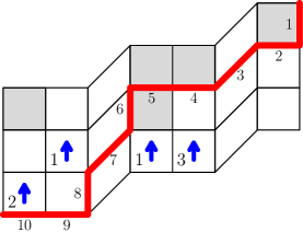
Figure 10. A CRT of type $\mu=0212201022$ that corresponds to the two-line queue of Figure 9.

Proof.

We present the bijection. Given a CRT $T$ of type $\mu\in\operatorname{States}(k,r,\ell)$, we label the rows and columns of $T$ by the label of the corresponding edge in $P(\mu)$. We build a queue $Q$ from $T$. We first fill the two rows of the queue with the following rules. For each $i$, the site in column $i$ of the bottom row is empty if and only if $\mu_{i}=0$; otherwise it contains a ball. The site in column $i$ of the top row is empty if and only if one of the following occurs:

• $\mu_{i}=1$,

• $\mu_{i}=0$ and the row $i$ of $T$ is empty, or

• $\mu_{i}=2$ and the column $i$ of $T$ contains an arrow which has the largest label in its row.

We now explain how to match the balls in $Q$.

• A restricted top row ball in column $i$ is matched to the bottom row ball in column $i$ if and only if the column $i$ of $T$ is empty.

• An unrestricted top row ball in column $i$ is matched to the the bottom row ball in column $j$ if and only if there exists in $T$ an arrow labelled $1$ in row $i$ and column $j$.

• A restricted top row ball in column $i$ is matched to the bottom row ball in column $j$ where $i\neq j$ if and only if there exists in $T$ an arrow labelled with some $k>1$ in column $j$, and in the same row there is an arrow labelled $k-1$ in column $i$.

It is a simple exercise to check that the weight of the $Q$ is equal to the weight of $T$, and the construction is bijective. ∎

Example of the bijection. We start with the CRT $T$ in Figure 10, where we have labeled the edges of $P(\mu)$ from 1 to 10 to correspond with the labels of the columns of the two-line queue $Q$. We first fill the bottom row of $Q$ by putting balls in all sites except for those in columns 1, 6, and 8, since those correspond to the vertical edge labels in $T$.

Now we fill the top row of $Q$. We put an empty site in column 1, as row 1 of $T$ is empty. The edges 3 and 6 or $P(\mu)$ are diagonal, so we put an empty site in columns 3 and 6 of $Q$. Finally the columns 5 and 9 of $T$ contain an arrow with the largest label in its corresponding row, and therefore we put an empty site in columns 5 and 9 of $Q$. The rest of the sites are filled with balls.

We proceed to match balls between the two rows of $Q$, starting with the empty columns of $T$. Column 2 of $T$ is empty, so the top row ball in column 2 is matched to the bottom row ball in column 2. Now we look at the non-empty rows of $T$ from bottom to top.

In row 8 and column 4 of $T$, there is an arrow labelled 1: therefore the top row ball in column 8 or $Q$ is matched with the bottom row ball in column 4.

In row 8 and column 10 of $T$, there is an arrow labelled 2: therefore the top row ball in column 4 of $Q$ is matched to the bottom row ball in column 10.

In row 8 and column 5 of $T$, there is an arrow labelled 3: therefore the top row ball in column 10 of $Q$ is matched to the bottom row ball in column 5.

We now look at row 6 of $T$. In column 9, there is an arrow labeled 1: therefore the top row ball in column 6 of $Q$ is matched to the bottom row ball in column 9.

Having recorded all the arrows in $T$, we get the two-line queue of Figure 9.

References

- [AAMP12] Chikashi Arita, Arvind Ayyer, Kirone Mallick, and Sylvain Prolhac. Generalized matrix ansatz in the multispecies exclusion process—the partially asymmetric case. J. Phys. A, 45(19):195001, 16, 2012.
- [AGS18] Erik Aas, Darij Grinberg, and Travis Scrimshaw. Multiline queues with spectral parameters. 2018. arXiv:1810.08157.
- [AL14] Arvind Ayyer and Svante Linusson. An inhomogeneous multispecies TASEP on a ring. Adv. in Appl. Math., 57:21–43, 2014.
- [AL18] Erik Aas and Svante Linusson. Continuous multi-line queues and TASEP. Ann. Inst. Henri Poincaré D, 5(1):127–152, 2018.
- [AM13] Chikashi Arita and Kirone Mallick. Matrix product solution of an inhomogeneous multi-species TASEP. J. Phys. A, 46(8):085002, 11, 2013.
- [Ang06] Omer Angel. The stationary measure of a 2-type totally asymmetric exclusion process. J. Combin. Theory Ser. A, 113(4):625–635, 2006.
- [BC14] Alexei Borodin and Ivan Corwin. Macdonald processes. Probab. Theory Related Fields, 158(1-2):225–400, 2014.
- [BE04] R. Brak and J. W. Essam. Asymmetric exclusion model and weighted lattice paths. J. Phys. A, 37(14):4183–4217, 2004.
- [Can17] Luigi Cantini. Asymmetric simple exclusion process with open boundaries and Koornwinder polynomials. Ann. Henri Poincaré, 18(4):1121–1151, 2017.
- [CdGW] Luigi Cantini, Jan de Gier, and Michael Wheeler. Matrix product and sum rule for Macdonald polynomials. FPSAC abstract.
- [CdGW15] Luigi Cantini, Jan de Gier, and Michael Wheeler. Matrix product formula for Macdonald polynomials. J. Phys. A, 48(38):384001, 25, 2015.
- [Che95a] Ivan Cherednik. Double affine Hecke algebras and Macdonald’s conjectures. Ann. of Math. (2), 141(1):191–216, 1995.
- [Che95b] Ivan Cherednik. Nonsymmetric Macdonald polynomials. Internat. Math. Res. Notices, (10):483–515, 1995.
- [CMW17] Sylvie Corteel, Olya Mandelshtam, and Lauren Williams. Combinatorics of the two-species ASEP and Koornwinder moments. Adv. Math., 321:160–204, 2017.
- [CMW18] Sylvie Corteel, Olya Mandelshtam, and Lauren Williams. From multiline queues to macdonald polynomials via the exclusion process. 2018. arXiv:?
- [CW07] Sylvie Corteel and Lauren K. Williams. Tableaux combinatorics for the asymmetric exclusion process. Adv. in Appl. Math., 39(3):293–310, 2007.
- [CW11] Sylvie Corteel and Lauren K. Williams. Tableaux combinatorics for the asymmetric exclusion process and Askey-Wilson polynomials. Duke Math. J., 159(3):385–415, 2011.
- [CW15] Sylvie Corteel and Lauren Williams. Macdonald-Koornwinder moments and the two-species exclusion process. to appear in Selecta Mathematica, 2015.
- [DEHP93] B. Derrida, M. R. Evans, V. Hakim, and V. Pasquier. Exact solution of a D asymmetric exclusion model using a matrix formulation. J. Phys. A, 26(7):1493–1517, 1993.
- [DJLS93] B. Derrida, S. A. Janowsky, J. L. Lebowitz, and E. R. Speer. Exact solution of the totally asymmetric simple exclusion process: shock profiles. J. Statist. Phys., 73(5-6):813–842, 1993.
- [DS05] Enrica Duchi and Gilles Schaeffer. A combinatorial approach to jumping particles. J. Combin. Theory Ser. A, 110(1):1–29, 2005.
- [EFM09] Martin R. Evans, Pablo A. Ferrari, and Kirone Mallick. Matrix representation of the stationary measure for the multispecies TASEP. J. Stat. Phys., 135(2):217–239, 2009.
- [FM07] Pablo A. Ferrari and James B. Martin. Stationary distributions of multi-type totally asymmetric exclusion processes. Ann. Probab., 35(3):807–832, 2007.
- [HHL05a] J. Haglund, M. Haiman, and N. Loehr. A combinatorial formula for Macdonald polynomials. J. Amer. Math. Soc., 18(3):735–761, 2005.
- [HHL05b] J. Haglund, M. Haiman, and N. Loehr. Combinatorial theory of Macdonald polynomials. I. Proof of Haglund’s formula. Proc. Natl. Acad. Sci. USA, 102(8):2690–2696, 2005.
- [HHL08] J. Haglund, M. Haiman, and N. Loehr. A combinatorial formula for nonsymmetric Macdonald polynomials. Amer. J. Math., 130(2):359–383, 2008.
- [KM17] Ryan Kaliszewski and Jennifer Morse. Colorful combinatorics and macdonald polynomials. 2017. arXiv:1710.00801.
- [KMO15] Atsuo Kuniba, Shouya Maruyama, and Masato Okado. Multispecies TASEP and combinatorial . J. Phys. A, 48(34):34FT02, 19, 2015.
- [Lig75] Thomas M. Liggett. Ergodic theorems for the asymmetric simple exclusion process. Trans. Amer. Math. Soc., 213:237–261, 1975.
- [Lig05] Thomas M. Liggett. Interacting particle systems. Classics in Mathematics. Springer-Verlag, Berlin, 2005. Reprint of the 1985 original.
- [Mac95] I. G. Macdonald. Symmetric functions and Hall polynomials. Oxford Mathematical Monographs. The Clarendon Press, Oxford University Press, New York, second edition, 1995. With contributions by A. Zelevinsky, Oxford Science Publications.
- [Man17] Olya Mandelshtam. Toric tableaux and the inhomogeneous two-species tasep on a ring. 2017. arXiv:1707.02663.
- [Mar18] James B. Martin. Stationary distributions of the multi-type ASEPs. 2018. arXiv:1810.10650.
- [MGP68] J Macdonald, J Gibbs, and A Pipkin. Kinetics of biopolymerization on nucleic acid templates. Biopolymers, 6, 1968.
- [Opd95] Eric M. Opdam. Harmonic analysis for certain representations of graded Hecke algebras. Acta Math., 175(1):75–121, 1995.
- [PEM09a] S. Prolhac, M. R. Evans, and K. Mallick. The matrix product solution of the multispecies partially asymmetric exclusion process. J. Phys. A, 42(16):165004, 25, 2009.
- [PEM09b] S. Prolhac, M. R. Evans, and K. Mallick. The matrix product solution of the multispecies partially asymmetric exclusion process. J. Phys. A, 42(16):165004, 25, 2009.
- [Spi70] Frank Spitzer. Interaction of Markov processes. Advances in Math., 5:246–290 (1970), 1970.
- [The18] The Sage Developers. SageMath, the Sage Mathematics Software System (Version v8.2), 2018. http://www.sagemath.org.
- [USW04] Masaru Uchiyama, Tomohiro Sasamoto, and Miki Wadati. Asymmetric simple exclusion process with open boundaries and Askey-Wilson polynomials. J. Phys. A, 37(18):4985–5002, 2004.