Regime Transition in the Energy Cascade of Rotating Turbulence

Abstract

Transition from a split to a forward kinetic energy cascade system is explored in the context of rotating turbulence using direct numerical simulations with a three-dimensional isotropic random force uncorrelated with the velocity field. Our parametric study covers confinement effects in large aspect ratio domains and a broad range of rotation rates. The data here presented add substantially to previous works, which, in contrast, focused on smaller and shallower domains. Results indicate that for fixed geometrical dimensions the Rossby number acts as a control parameter, whereas for a fixed Rossby number the product of the domain size along the rotation axis and forcing wavenumber governs the amount of energy that cascades inversely. The regime transition criterion hence depends on both control parameters.

I Introduction

The energy cascade is the fundamental mechanism in turbulent flows that describes the energy exchange between the various scales of motion (Frisch, 1995). A forward cascade from large to small scales is commonly observed in three-dimensional (3D) flows, whereas an inverse energy cascade from small towards large scales is the hallmark of two-dimensional (2D) flows (Alexakis and Biferale, 2018; Boffetta and Ecke, 2012). Predicting the energy cascade direction, therefore, requires anticipating if, for a given set of control parameters, the resulting flow field resembles best 3D or 2D flow dynamics. In lack of analytical predictions, a typical approach consists of carefully designing numerical experiments, where the system’s parameters are individually varied to produce a phase transition diagram. Throughout this study we consider a large number of forced direct numerical simulations (DNS) and analyze the influence of geometric confinement and system rotation on the cascade direction in homogeneous rotating turbulence.

Inertial waves, i.e. plane wave solutions to the linearized Navier-Stokes equations, can modulate the energy transfer in rotating turbulence (Greenspan, 1968; Godeferd et al., 2015). By considering high rotation rates and exploiting the fact that rotating turbulence is a multi-timescale problem, Waleffe (1993) suggested that the nonlinear dynamics are modified by wave interactions. Resonant wave interactions can explain the favored energy transfer towards horizontal modes, whereas non-resonant wave interactions are considered to damp and inhibit the triadic interactions typical of homogeneous turbulence (Cambon et al., 1997; Smith and Waleffe, 1999). This mechanism also persists at lower rotation rates due to homochirical interactions that transfer energy into the plane orthogonal to the rotation axis (Buzzicotti et al., 2018). As a consequence, when rotating homogeneous flows are forced at wavenumber $\kappa_{f}$, the injected energy can cascade both to larger ($\kappa<\kappa_{f}$) and smaller scales ($\kappa>\kappa_{f}$); this is hereafter referred to as split energy cascade. These findings help to explain the preferential upscale of energy typically found in numerical and experimental investigations of rotating turbulent flows (Yeung and Zhou, 1998; Smith and Waleffe, 1999; Mininni et al., 2009; Moisy et al., 2011; Mininni et al., 2012; Delache et al., 2014). Nevertheless, we must bear in mind that a large network of triadic interactions as in the Navier-Stokes equations can evolve differently than a set of isolated triads, as previously pointed out in Refs. (Linkmann and Dallas, 2017; Moffatt, 2014).

Among different theories that elucidate the phenomenon of rotating turbulence, the work of Galtier (2003) is regarded as an important contribution. Based on wave turbulence theory, which deals with systems where interactions are governed by waves, he derived scaling laws for the energy spectrum. These laws were also shown to follow from phenomenological arguments for the spectral transfer time — a typical energy transfer timescale. For infinitely large domains, as required by wave turbulence theory (Nazarenko, 2011), the weak inertial-wave theory of Galtier (2003) predicts that energy cascades forward and to small scales. However, a passage from a split to a forward energy cascade system by approaching the large-box limit has not yet been confirmed by DNS.

In the absence of rotation, however, the geometrical dimensions of the system itself influences the energy cascade direction. Using a two-dimensional two-component (2D2C) horizontal force, Smith et al. (1996) and Celani et al. (2010) found that the ratio $L_{3}/\ell_{f}$, where $L_{3}$ is the vertical domain extension and $\ell_{f}$ is the forcing lengthscale, is a governing control parameter. They showed that large $L_{3}/\ell_{f}$ results in a forward energy cascade, whereas inverse energy transfer was triggered and split the energy cascade for $L_{3}/\ell_{f}\leq 1/2$. More recently, numerical simulations by Benavides and Alexakis (2017) explored transitions in a thin layer of fluid subjected to free-slip boundary conditions. Transition from a forward to a split energy cascade was shown to be critical and depend on the ratio of forcing lengthscale to wall separation.

Regime transitions in rotating homogeneous turbulence are therefore affected by geometrical dimensions and rotation rate. Deusebio et al. (2014) studied hyperviscous fluids in rotating small aspect ratio domains subjected to 2D2C forcing and found that large rotation rates as well as small $L_{3}/\ell_{f}$ suppress enstrophy production and induce an inverse energy cascade. Their data proves, at least for weak rotation rates, that transition from a split to a forward cascade is possible by controlling either rotation rate or domain size. For strong rotation, however, almost the entire injected energy cascaded inversely. Although transition was not observed, they hypothesized that it could still take place for sufficiently large $L_{3}/\ell_{f}$. This conjecture, however, remains to be verified by either forcing smaller flow scales or by increasing the domain size (Seshasayanan and Alexakis, 2018).

The present work sheds light on the question whether a transition from a split to a forward cascade system always exists in forced homogeneous rotating turbulence. We conduct a systematic parametric study that covers several rotation rates and an unprecedented range of geometric confinements by considering strongly elongated domains and large forcing wavenumbers $\kappa_{f}$. This new database is complementary to previous studies, which focused on the confinement induced transition in smaller and shallower domains. Through large-scale forcing, we construct isotropic flow fields that are posteriorly subjected to rotation. Differently from previous studies, we employ a three-dimensional three-component (3D3C) forcing scheme that by design provides a constant energy input independent of the velocity field. We believe this results in a neater and more general framework where anisotropy originates solely from rotation.

II Methodology and Governing Parameters

We solve the incompressible Navier-Stokes equations in a frame rotating at rate $\boldsymbol{\Omega}$:

$$\nabla\cdot\mathbf{u} =0,$$ (1)

$$\frac{\partial\mathbf{u}}{\partial t}+(2\,\boldsymbol{\Omega}+\boldsymbol{\omega})\times\mathbf{u} =-\nabla q+\nu\nabla^{2}\mathbf{u}+\mathbf{f}.$$ (2)

Here, $\mathbf{u}$, $\boldsymbol{\omega}$ and $\mathbf{f}$ are velocity, vorticity and an external force, respectively. The reduced pressure into which the centrifugal force is incorporated is given by $q$, and $\nu$ denotes the kinematic viscosity.

Equations 1 and 2 are discretized in space by a dealiased Fourier pseudo-spectral method (2/3-rule) in a triply-periodic domain of size $2\pi\mathcal{L}_{1}\times 2\pi\mathcal{L}_{2}\times 2\pi\mathcal{L}_{3}$ (Orszag, 1971; Pekurovsky, 2012). The rotation axis is assumed aligned with the vertical direction, i.e. $\boldsymbol{\Omega}=\Omega\,\mathbf{\hat{e}}_{3}$, and we restrict ourselves to cases where the domain size in the direction perpendicular to the axis of rotation are equal: $\mathcal{L}_{1}=\mathcal{L}_{2}=\mathcal{L}_{\perp}=1$. Accordingly, $\mathcal{L}_{\mkern 3.0mu\vphantom{\perp}\vrule depth=0.0pt\mkern 2.0mu\vrule depth=0.0pt\mkern 3.0mu}$ replaces $\mathcal{L}_{3}$ to denote the domain size in the direction parallel to the rotation axis, and can be arbitrarily chosen. We use Rogallo’s integrating factor technique for exact time integration of the viscous and Coriolis terms and a third-order Runge-Kutta scheme for the nonlinear terms (Rogallo, 1977; Morinishi et al., 2001).

The external force $\mathbf{f}$ injects energy to the system at rate $\varepsilon_{I}$, see Ref. (Alvelius, 1999). The force’s spectrum $F(\kappa)$, from which $\mathbf{f}$ in Eq. 2 is assembled, is Gaussian distributed, centered around a wavenumber $\kappa_{f}$ and has standard deviation $c=0.5$: $F(\kappa)=A\exp(-(\kappa-\kappa_{f})^{2}/c)$.

Table 1: List of direct numerical simulations at $\mathrm{Re_{\varepsilon}}\approx 55$. The $\mathrm{Ro_{\varepsilon}}$ numbers are given in the footnote.

Case	$\kappa_{f}\mathcal{L}_{\perp}$	$\kappa_{f}\mathcal{L}_{\mkern 3.0mu\vphantom{\perp}\vrule depth=0.0pt\mkern 2.0mu\vrule depth=0.0pt\mkern 3.0mu}$	$A_{r}$	$N_{p}$
kf02-a01	2	2	1	$192^{3}$
kf04-a01	4	4	1	$384^{3}$
kf04-a02	4	8	2	$384^{2}\times 768$
kf04-a04	4	16	4	$384^{2}\times 1536$
kf04-a08	4	32	8	$384^{2}\times 3072$
kf04-a16	4	64	16	$384^{2}\times 6144$
kf04-a32	4	128	32	$384^{2}\times 12288$
kf08-a01 a	8	8	1	$768^{3}$
kf08-a02	8	16	2	$768^{2}\times 1536$
kf08-a04	8	32	4	$768^{2}\times 3072$
kf08-a08	8	64	8	$768^{2}\times 6144$
kf08-a16	8	128	16	$768^{2}\times 12288$
kf16-a01	16	16	1	$1536^{3}$
kf16-a02	16	32	2	$1536^{2}\times 3072$
kf16-a04	16	64	4	$1536^{2}\times 6144$
kf32-a01	32	32	1	$3072^{3}$

For given $\kappa_{f}$ and $c$, the prefactor $A$ is uniquely determined from the desired energy input rate $\varepsilon_{I}$. In the absence of rotation, we obtain isotropic velocity fields and a balance between energy input rate and viscous dissipation, i.e. $\varepsilon_{I}=\varepsilon_{\nu}$. This forcing scheme ensures through projection that the force and velocity field are uncorrelated at every instant of time (Alvelius, 1999). As a consequence, $\varepsilon_{I}$ is solely determined by the force-force correlation and is independent of the velocity field. Thus, we can define a priori true control parameters from which the governing non-dimensional numbers are derived.

The domain size, $\mathcal{L}_{\mkern 3.0mu\vphantom{\perp}\vrule depth=0.0pt\mkern 2.0mu\vrule depth=0.0pt\mkern 3.0mu}$ and $\mathcal{L}_{\perp}$, the forcing wavenumber $\kappa_{f}$, the viscosity $\nu$, the rotation rate $\Omega$ and the energy input rate $\varepsilon_{I}$ can all be freely chosen. Regarding $\varepsilon_{I}$, it could be additionally decomposed in three contributions stemming from the power injected in each direction. However, because the forcing is isotropic, it is sufficient to consider the total power input $\varepsilon_{I}$ only. These six parameters $\{\kappa_{f},\nu,\varepsilon_{I},\Omega,\mathcal{L}_{\perp},\mathcal{L}_{\mkern 3.0mu\vphantom{\perp}\vrule depth=0.0pt\mkern 2.0mu\vrule depth=0.0pt\mkern 3.0mu}\}$ form the set of true control parameters and are the basis for the non-dimensional similarity numbers. The characteristic length, velocity and time-scale follow naturally as $\ell_{f}=\kappa_{f}^{-1}$, $u_{f}=\varepsilon_{I}^{1/3}\,\,\kappa_{f}^{-1/3}$, and $\tau_{f}=\kappa_{f}^{-2/3}\,\,\varepsilon_{I}^{-1/3}$, respectively. In addition, a timescale based on the rotation rate is taken as $\tau_{\Omega}=1/(2\Omega)$.

The Reynolds and Rossby numbers are now unambiguously defined as

$$\mathrm{Re_{\varepsilon}}=\frac{\varepsilon_{I}^{1/3}\,\,\kappa_{f}^{-4/3}}{\nu}\quad\mbox{and}\quad\mathrm{Ro_{\varepsilon}}=\frac{\kappa_{f}^{2/3}\varepsilon_{I}^{1/3}}{2\Omega}.$$ (3)

From the problem’s geometry and the forcing wavenumber, we define two other non-dimensional numbers, i.e. $\kappa_{f}\mathcal{L}_{\perp}$ and $\kappa_{f}\mathcal{L}_{\mkern 3.0mu\vphantom{\perp}\vrule depth=0.0pt\mkern 2.0mu\vrule depth=0.0pt\mkern 3.0mu}$. Hence, we obtain a set of four independent governing non-dimensional numbers that fully describes our numerical experiments: $\mathrm{Re_{\varepsilon}}$, $\mathrm{Ro_{\varepsilon}}$, $\kappa_{f}\mathcal{L}_{\perp}$ and $\kappa_{f}\mathcal{L}_{\mkern 3.0mu\vphantom{\perp}\vrule depth=0.0pt\mkern 2.0mu\vrule depth=0.0pt\mkern 3.0mu}$. As the final goal is to investigate dimensional and rotational effects on forced homogeneous rotating turbulence, we fix $\mathrm{Re_{\varepsilon}}$ and allow $\mathrm{Ro_{\varepsilon}}$, $\kappa_{f}\mathcal{L}_{\mkern 3.0mu\vphantom{\perp}\vrule depth=0.0pt\mkern 2.0mu\vrule depth=0.0pt\mkern 3.0mu}$ and $\kappa_{f}\mathcal{L}_{\perp}$ to vary. We remark that this set is not unique and other non-dimensional groups exist. For instance, $\mathrm{Re_{\varepsilon}}$ and $\mathrm{Ro_{\lambda}}$ could be combined to form the micro-scale Rossby number $\mathrm{Ro_{\lambda}}=\mathrm{Re_{\varepsilon}}^{1/2}\mathrm{Ro_{\lambda}}$ (ratio of rotation and Kolmogorov timescale (Cambon et al., 1997)) or $\kappa_{f}\mathcal{L}_{\mkern 3.0mu\vphantom{\perp}\vrule depth=0.0pt\mkern 2.0mu\vrule depth=0.0pt\mkern 3.0mu}$ and $\kappa_{f}\mathcal{L}_{\perp}$ could be related to obtain the domain’s aspect ratio $A_{r}=\mathcal{L}_{\mkern 3.0mu\vphantom{\perp}\vrule depth=0.0pt\mkern 2.0mu\vrule depth=0.0pt\mkern 3.0mu}/\mathcal{L}_{\perp}$. Initial conditions were generated by performing DNS of non-rotating forced isotropic turbulence. We started from a zero-velocity field and marched in time until a fully developed steady-state was achieved. After the initial transient statistics, were sampled over at least $24\,\tau_{f}$, corresponding to approximately ten large-eddy turnover times. Following this procedure, a reference isotropic solution was computed for every entry in Tab. 1.

The initially imposed $\mathrm{Re_{\varepsilon}}\approx 55$ ultimately led to homogeneous non-rotating turbulent fields with a characteristic Taylor micro-scale Reynolds number $\mathrm{Re_{\lambda}}\approx 68$. The spatial resolution in terms of the Kolmogorov lengthscale $\eta$ was kept constant throughout this study, i.e. $\kappa_{max}\eta\approx 1.5$, where $\kappa_{max}$ is the largest represented wavenumber. For the case with largest $\kappa_{f}\mathcal{L}_{\mkern 3.0mu\vphantom{\perp}\vrule depth=0.0pt\mkern 2.0mu\vrule depth=0.0pt\mkern 3.0mu}$, the integral lengthscale in the direction of rotation is about $600$ times smaller than the respective domain size.

Figure 1 compares the 3D spherically averaged energy spectrum $E(\kappa)$ for cases with aspect ratio $A_{r}=1$, which contain “a01” in its name description, and two additional simulations with $A_{r}=16$ and $A_{r}=32$ (cases kf04-a32 and kf08-a16 in Tab. 1). This data proves the equivalence between initial conditions for DNS forced at different wavenumbers and those computed with distinct $\kappa_{f}\mathcal{L}_{\mkern 3.0mu\vphantom{\perp}\vrule depth=0.0pt\mkern 2.0mu\vrule depth=0.0pt\mkern 3.0mu}$ and $\kappa_{f}\mathcal{L}_{\perp}$. We find that the energy spectra perfectly coincide and that $E(\kappa)$ scales best with $\kappa^{2}$ at wavenumbers $\kappa<\kappa_{f}$, in agreement with Ref. (Dallas et al., 2015). The obtained isotropic velocity fields were used as initial condition for the simulations with different rotation rates. The statistical variability of the results for small domains was reduced by ensemble averaging. For the smallest domain kf02-a01 we ensemble averaged $10$ independent realizations and cases kf04 with $A_{r}>1$ are averages of $3$ realizations. For all other cases, the data represents a single numerical experiment.

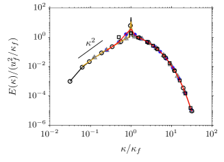
Figure 1: Three-dimensional spherically averaged energy spectrum of the initial condition: kf02-a01 ($\square$), kf04-a01 ( ), kf08-a01 (+), kf16-a01 ( ), kf32-a01 ( $\boldsymbol{\circ}$ ), kf04-a32 ($*$) kf08-a16 ($\triangle$)

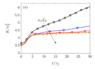
(a)

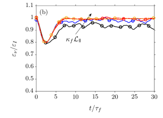
(b)

Figure 2: Time evolution of box-averaged kinetic energy (a) and energy dissipation rate (b) for $\mathrm{Ro_{\varepsilon}}\approx 0.31$ (weak rotation). Lines corresponding to same $\kappa_{f}\mathcal{L}_{\perp}$ are grouped by color: $\kappa_{f}\mathcal{L}_{\perp}=2$ ($\blacksquare$), $\kappa_{f}\mathcal{L}_{\perp}=4$ ($\blacksquare$), $\kappa_{f}\mathcal{L}_{\perp}=8$ ($\blacksquare$), $\kappa_{f}\mathcal{L}_{\perp}=16$ ($\blacksquare$), Lines corresponding to the same $A_{r}$ are grouped by line types: $A_{r}=1$ ( $\boldsymbol{\circ}$ ), $A_{r}=8$ (     ), cf. Tab. 1.

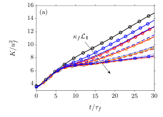
(a)

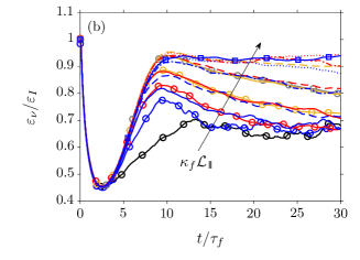
(b)

Figure 3: Time evolution of box-averaged kinetic energy (a) and energy dissipation rate (b) for $\mathrm{Ro_{\varepsilon}}\approx 0.06$ (strong rotation). Lines corresponding to same $\kappa_{f}\mathcal{L}_{\perp}$ are grouped by color: $\kappa_{f}\mathcal{L}_{\perp}=2$ ($\blacksquare$), $\kappa_{f}\mathcal{L}_{\perp}=4$ ($\blacksquare$), $\kappa_{f}\mathcal{L}_{\perp}=8$ ($\blacksquare$), $\kappa_{f}\mathcal{L}_{\perp}=16$ ($\blacksquare$), $\kappa_{f}\mathcal{L}_{\perp}=32$ ($\blacksquare$). Lines corresponding to the same $A_{r}$ are grouped by line types: $A_{r}=1$ ( $\boldsymbol{\circ}$ ), $A_{r}=2$ ( ), $A_{r}=4$ (     ), $A_{r}=8$ (     ), $A_{r}=16$ (           ), $A_{r}=32$ ( $\square$ ), cf. Tab. 1.

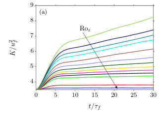
(a)

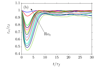
(b)

Figure 4: Time evolution of box-averaged kinetic energy (a) and energy dissipation rate (b) for $\kappa_{f}\mathcal{L}_{\perp}=8$ and $\kappa_{f}\mathcal{L}_{\mkern 3.0mu\vphantom{\perp}\vrule depth=0.0pt\mkern 2.0mu\vrule depth=0.0pt\mkern 3.0mu}=64$. Different line colors correspond to the range $0.06<\mathrm{Ro_{\varepsilon}}<1.25$, see Tab. 1.

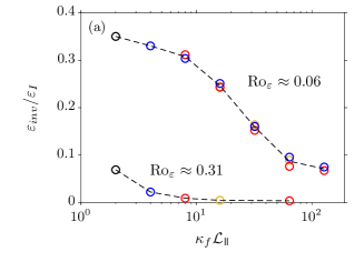
(a)

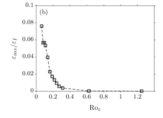
(b)

Figure 5: Phase transition diagram for weak and strong rotation and varying geometrical dimensions (a) and for constant geometrical dimension and varying $\mathrm{Ro_{\varepsilon}}$ (b). Color scheme of (a) is the same as in Fig. 3. In (a), the data point for $\kappa_{f}\mathcal{L}_{\perp}=\kappa_{f}\mathcal{L}_{\mkern 3.0mu\vphantom{\perp}\vrule depth=0.0pt\mkern 2.0mu\vrule depth=0.0pt\mkern 3.0mu}=32$ (case kf32-a01) is almost identical to case kf04-a08 ($\kappa_{f}\mathcal{L}_{\perp}=4$; $\kappa_{f}\mathcal{L}_{\mkern 3.0mu\vphantom{\perp}\vrule depth=0.0pt\mkern 2.0mu\vrule depth=0.0pt\mkern 3.0mu}=32$), and is therefore not visible.

III Results

First we assess the effects of geometrical dimension and rotation on the time evolution of box-averaged kinetic energy $K$ and viscous dissipation $\varepsilon_{\nu}$. The non-dimensional geometric parameters $\kappa_{f}\mathcal{L}_{\perp}$ and $\kappa_{f}\mathcal{L}_{\mkern 3.0mu\vphantom{\perp}\vrule depth=0.0pt\mkern 2.0mu\vrule depth=0.0pt\mkern 3.0mu}$ are varied for two fixed rotation rates: weak ($\mathrm{Ro_{\varepsilon}}=0.31$; Fig. 2) and strong ($\mathrm{Ro_{\varepsilon}}=0.06$; Fig. 3). Additionally, for a fixed and large domain, $\kappa_{f}\mathcal{L}_{\perp}=8$ and $\kappa_{f}\mathcal{L}_{\mkern 3.0mu\vphantom{\perp}\vrule depth=0.0pt\mkern 2.0mu\vrule depth=0.0pt\mkern 3.0mu}=64$ (case kf08-a08; Fig. 4), we investigate the Rossby number range $0.06<\mathrm{Ro_{\varepsilon}}<1.25$. For more details about the simulation parameters, please refer to Tab. 1.

All cases undergo a transient of roughly $10\,\tau_{f}$ from the onset of rotation (Figs. 2, 3 and 4), which converges towards a unique solution for sufficiently large $\kappa_{f}\mathcal{L}_{\mkern 3.0mu\vphantom{\perp}\vrule depth=0.0pt\mkern 2.0mu\vrule depth=0.0pt\mkern 3.0mu}$. We find that the results are independent of the transversal domain size for $\kappa_{f}\mathcal{L}_{\perp}\geq 4$; see Fig. 3, where the lines for different $\kappa_{f}\mathcal{L}_{\perp}$ and identical $\kappa_{f}\mathcal{L}_{\mkern 3.0mu\vphantom{\perp}\vrule depth=0.0pt\mkern 2.0mu\vrule depth=0.0pt\mkern 3.0mu}$ coincide. Departing from an isotropic state, where the energy cascade is strictly forward ($\varepsilon_{\nu}/\varepsilon_{I}=1$), $\varepsilon_{\nu}$ decreases monotonically until it is lowest at approximately $3\,\tau_{f}$ (Figs. 2b, 3b and 4b). For fixed $\mathrm{Ro_{\varepsilon}}$, Figs. 2b and 3b show that both $\kappa_{f}\mathcal{L}_{\perp}$ and $\kappa_{f}\mathcal{L}_{\mkern 3.0mu\vphantom{\perp}\vrule depth=0.0pt\mkern 2.0mu\vrule depth=0.0pt\mkern 3.0mu}$ have no influence on the minimum of $\varepsilon_{\nu}$. On the other hand, Fig. 4b suggests a direct proportionality between the minimum value of $\varepsilon_{\nu}$ and $\mathrm{Ro_{\varepsilon}}$.

After $t\approx 3\,\tau_{f}$, $\varepsilon_{\nu}$ increases towards $\varepsilon_{I}$. Nevertheless, the strong and weak rotation cases lead to a different final state for $\varepsilon_{\nu}$. While increasing $\kappa_{f}\mathcal{L}_{\mkern 3.0mu\vphantom{\perp}\vrule depth=0.0pt\mkern 2.0mu\vrule depth=0.0pt\mkern 3.0mu}$ restores $\varepsilon_{\nu}=\varepsilon_{I}$ for the weak rotating case (Fig. 2b), the imbalance $\varepsilon_{\nu}<\varepsilon_{I}$, although lower than $0.075\,\varepsilon_{I}$ for $\kappa_{f}\mathcal{L}_{\mkern 3.0mu\vphantom{\perp}\vrule depth=0.0pt\mkern 2.0mu\vrule depth=0.0pt\mkern 3.0mu}=128$, persists up to the final time for the strong rotating case (Fig. 3b). Similarly to Fig. 2b, increasing $\mathrm{Ro_{\varepsilon}}$ reestablishes a forward energy cascade for a fixed domain size (Fig. 4b). After the initial transient ($t>10\,\tau_{f}$), $\varepsilon_{\nu}$ follows mostly a slow linear decay (Fig. 3b) or remains nearly constant (Figs. 2b and 4b). Consequently, $K$, which evolves in time as ${\mbox{d}{K}}/{\mbox{d}{t}}=\varepsilon_{I}-\varepsilon_{\nu}$, grows quasi-linearly (Figs. 2a, 3a and 4a). Based on this idea we define the inverse energy flux $\varepsilon_{inv}=\varepsilon_{I}-\varepsilon_{\nu}$ from the imbalance between energy injection rate and viscous dissipation. To estimate $\varepsilon_{inv}$, which is equal to the local slope of $K(t)$, a linear least-square fit is applied to $15\,\tau_{f}<t<30\,\tau_{f}$ in the time evolution of $K$ (Figs. 2a, 3a and 4a). The r.m.s. residual between the actual and fitted data indicates that the linear regression model is appropriate. For the worst case, kf04-a08, the r.m.s. residual is $0.65\%$ of the mean value. Assuming that the linear law is exact and the noise is essentially Gaussian, one obtains $0.0004$ for the standard error of the slope coefficient. Results for the inverse energy flux are thus shown in Figs. 5 and 6 in form of a phase transition diagram.

From Fig. 5a, we see that the inverse energy flux $\varepsilon_{inv}$ decreases monotonically with $\kappa_{f}\mathcal{L}_{\mkern 3.0mu\vphantom{\perp}\vrule depth=0.0pt\mkern 2.0mu\vrule depth=0.0pt\mkern 3.0mu}$ for both $\mathrm{Ro_{\varepsilon}}\approx 0.31$ and $\mathrm{Ro_{\varepsilon}}\approx 0.06$. Moreover, results for the strong rotating case suggest that increasing $\kappa_{f}\mathcal{L}_{\perp}$ while retaining $\kappa_{f}\mathcal{L}_{\mkern 3.0mu\vphantom{\perp}\vrule depth=0.0pt\mkern 2.0mu\vrule depth=0.0pt\mkern 3.0mu}$ leads to negligible differences in $\varepsilon_{inv}$ — see the overlapping circles with different colors for $\mathrm{Ro_{\varepsilon}}\approx 0.06$. Transition from a split to a forward cascade system occurs gradually. For $\mathrm{Ro_{\varepsilon}}\approx 0.31$ and $\kappa_{f}\mathcal{L}_{\mkern 3.0mu\vphantom{\perp}\vrule depth=0.0pt\mkern 2.0mu\vrule depth=0.0pt\mkern 3.0mu}=64$ less than $0.004\,\varepsilon_{I}$ is transferred in the inverse direction, whereas for $\mathrm{Ro_{\varepsilon}}\approx 0.06$ a split cascade is still present at $\kappa_{f}\mathcal{L}_{\mkern 3.0mu\vphantom{\perp}\vrule depth=0.0pt\mkern 2.0mu\vrule depth=0.0pt\mkern 3.0mu}=128$. For a fixed domain size with $\kappa_{f}\mathcal{L}_{\perp}=8$ and $\kappa_{f}\mathcal{L}_{\mkern 3.0mu\vphantom{\perp}\vrule depth=0.0pt\mkern 2.0mu\vrule depth=0.0pt\mkern 3.0mu}=64$ (case kf08-a08; Fig. 5b), $\varepsilon_{inv}$ is continuously suppressed for increasing $\mathrm{Ro_{\varepsilon}}$ and transition to a forward cascade system occurs in the vicinity of $\mathrm{Ro_{\varepsilon}}=1$.

A question that follows from these results is for which combination of governing non-dimensional parameters regime transition occurs. From literature, a possible criteria is $\mathrm{Ro_{\varepsilon}}\kappa_{f}\mathcal{L}_{\mkern 3.0mu\vphantom{\perp}\vrule depth=0.0pt\mkern 2.0mu\vrule depth=0.0pt\mkern 3.0mu}=C$, where $C$ is a constant (Seshasayanan and Alexakis, 2018; Alexakis and Biferale, 2018). To test this hypothesis, Fig. 6 presents the data from Fig. 5, but juxtaposed in a single diagram and scaled accordingly with $\mathrm{Ro_{\varepsilon}}\kappa_{f}\mathcal{L}_{\mkern 3.0mu\vphantom{\perp}\vrule depth=0.0pt\mkern 2.0mu\vrule depth=0.0pt\mkern 3.0mu}$. The curves for different $\mathrm{Ro_{\varepsilon}}$ do not line up; hence, this criteria disagrees with our data. A discussion on a possible reason is given in the next section.

Now we turn our attention to the influence of $\kappa_{f}\mathcal{L}_{\mkern 3.0mu\vphantom{\perp}\vrule depth=0.0pt\mkern 2.0mu\vrule depth=0.0pt\mkern 3.0mu}$ and $\kappa_{f}\mathcal{L}_{\perp}$ on the spectral energy flux and energy spectra. Hereafter we present results for the strong rotating case with $\mathrm{Ro_{\varepsilon}}\approx 0.06$ only, as differences are more pronounced than in the weak rotating case. Although we show instantaneous data at $t=30\,\tau_{f}$, the trend described in what follows also holds for other instants of time. Conservation of energy requires the portion of the injected energy that is not dissipated to be accumulated. By analyzing the spectral energy flux $\Pi(\kappa)$, we find that the net energy transfer $T(\kappa)=-{\mbox{d}{\Pi}}/{\mbox{d}{\kappa}}$ is positive for $\kappa<\kappa_{f}$. In other words, wavenumbers in this range gain energy and we observe an upscale energy transfer. Evidence is presented in Fig. 7, which also highlights how sensitive $\Pi(\kappa)$ is with respect to changes in $\kappa_{f}\mathcal{L}_{\mkern 3.0mu\vphantom{\perp}\vrule depth=0.0pt\mkern 2.0mu\vrule depth=0.0pt\mkern 3.0mu}$ and $\kappa_{f}\mathcal{L}_{\perp}$. In this regard, Fig. 7a, where $\kappa_{f}\mathcal{L}_{\mkern 3.0mu\vphantom{\perp}\vrule depth=0.0pt\mkern 2.0mu\vrule depth=0.0pt\mkern 3.0mu}$ is constant and $\kappa_{f}\mathcal{L}_{\perp}=\{8$, $16$, $32\}$, shows that the shape of $\Pi(\kappa)$ remains unaltered for different $\kappa_{f}\mathcal{L}_{\perp}$. On the other hand, varying $\kappa_{f}\mathcal{L}_{\mkern 3.0mu\vphantom{\perp}\vrule depth=0.0pt\mkern 2.0mu\vrule depth=0.0pt\mkern 3.0mu}$ from $16$ to $64$ while $\kappa_{f}\mathcal{L}_{\perp}$ is constant, reduces the magnitude of the inverse energy flux and the range of wavenumbers for which an upscale energy transfer takes place, see Fig. 7b. Therein, greater values of $\kappa_{f}\mathcal{L}_{\mkern 3.0mu\vphantom{\perp}\vrule depth=0.0pt\mkern 2.0mu\vrule depth=0.0pt\mkern 3.0mu}$ are also associated with an enhanced spectral energy flux for $\kappa>\kappa_{f}$. This is a consequence of the fixed energy input rate $\varepsilon_{I}$, which causes the step in $\Pi(\kappa)$ at $\kappa=\kappa_{f}$ to be the same for all cases.

The three-dimensional energy spectra $E(\kappa)$ for the same cases are shown in Fig. 8. Additionally, the energy spectrum of case kf32-a01 with $\kappa_{f}\mathcal{L}_{\mkern 3.0mu\vphantom{\perp}\vrule depth=0.0pt\mkern 2.0mu\vrule depth=0.0pt\mkern 3.0mu}=\kappa_{f}\mathcal{L}_{\perp}=32$ from Fig. 1 at the onset of rotation is included as reference. Figure 8a reinforces that $\kappa_{f}\mathcal{L}_{\mkern 3.0mu\vphantom{\perp}\vrule depth=0.0pt\mkern 2.0mu\vrule depth=0.0pt\mkern 3.0mu}$ dictates the degree of energy accumulation, as the curves for different $\kappa_{f}\mathcal{L}_{\perp}$ and constant $\kappa_{f}\mathcal{L}_{\mkern 3.0mu\vphantom{\perp}\vrule depth=0.0pt\mkern 2.0mu\vrule depth=0.0pt\mkern 3.0mu}$ overlap. In agreement with results in Fig. 7 for $\Pi(\kappa)$, we observe significantly higher levels of energy for $\kappa<\kappa_{f}$ with respect to the isotropic reference spectrum. These are reduced for increasing $\kappa_{f}\mathcal{L}_{\mkern 3.0mu\vphantom{\perp}\vrule depth=0.0pt\mkern 2.0mu\vrule depth=0.0pt\mkern 3.0mu}$, see Fig. 8b.

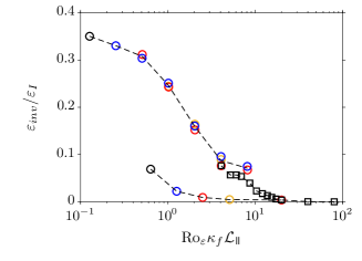
Figure 6: Phase transition diagram in terms of combined control parameter $\mathrm{Ro_{\varepsilon}}\kappa_{f}\mathcal{L}_{\mkern 3.0mu\vphantom{\perp}\vrule depth=0.0pt\mkern 2.0mu\vrule depth=0.0pt\mkern 3.0mu}$ for all data points of Fig. 5. Colored circles represent data from Fig. 5a, and squares data from Fig. 5b.

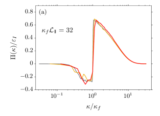
(a)

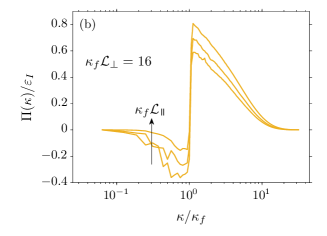
(b)

Figure 7: Spectral energy flux for $\mathrm{Ro_{\varepsilon}}\approx 0.06$ and cases with $\kappa_{f}\mathcal{L}_{\mkern 3.0mu\vphantom{\perp}\vrule depth=0.0pt\mkern 2.0mu\vrule depth=0.0pt\mkern 3.0mu}=32$ (a) and $\kappa_{f}\mathcal{L}_{\perp}=16$ (b). In (a), $\kappa_{f}\mathcal{L}_{\perp}=8$ ( ), $\kappa_{f}\mathcal{L}_{\perp}=16$ ( ) and $\kappa_{f}\mathcal{L}_{\perp}=32$ ( ). In (b), $\kappa_{f}\mathcal{L}_{\mkern 3.0mu\vphantom{\perp}\vrule depth=0.0pt\mkern 2.0mu\vrule depth=0.0pt\mkern 3.0mu}=16,32$ and $64$ ( ). Arrow denotes the direction of increase.

As for the distribution of energy in terms of $\kappa_{\mkern 3.0mu\vphantom{\perp}\vrule depth=0.0pt\mkern 2.0mu\vrule depth=0.0pt\mkern 3.0mu}$ and $\kappa_{\perp}$, Fig. 9 presents the two-dimensional energy spectrum $E(\kappa_{\perp},\kappa_{\mkern 3.0mu\vphantom{\perp}\vrule depth=0.0pt\mkern 2.0mu\vrule depth=0.0pt\mkern 3.0mu})$. Results are shown exclusively for case kf32-a01 with $\kappa_{f}\mathcal{L}_{\perp}=\kappa_{f}\mathcal{L}_{\mkern 3.0mu\vphantom{\perp}\vrule depth=0.0pt\mkern 2.0mu\vrule depth=0.0pt\mkern 3.0mu}=32$, as it contains most large scale resolution. The energy spectrum is non-dimensionalized with $2\pi\kappa_{\perp}$, in such a way that contour levels of isotropic spectra appear as circles centered at the origin. In agreement with previous works, Fig. 9 confirms that the kinetic energy has the tendency to accumulate at lower $\kappa_{\mkern 3.0mu\vphantom{\perp}\vrule depth=0.0pt\mkern 2.0mu\vrule depth=0.0pt\mkern 3.0mu}/\kappa_{f}$. Hence, $E(\kappa_{\perp},\kappa_{\mkern 3.0mu\vphantom{\perp}\vrule depth=0.0pt\mkern 2.0mu\vrule depth=0.0pt\mkern 3.0mu})$ is anisotropic and contour levels display an elliptical shape with major axis aligned with the $\kappa_{\perp}\text{-direction}$. This is observed even for high wavenumbers and suggests that all scales of motion are influenced by rotation; indeed, for this case, $\kappa_{\Omega}\eta=1.1$, where $\kappa_{\Omega}=(\Omega^{3}/\varepsilon_{I})^{1/2}$ is the Zeman wavenumber (Delache et al., 2014). At the same time, the energy input remains isotropic. See the inset for the imprint of the isotropic forcing scheme, which delineates the bright area located at $\kappa_{\mkern 3.0mu\vphantom{\perp}\vrule depth=0.0pt\mkern 2.0mu\vrule depth=0.0pt\mkern 3.0mu}^{2}+\kappa_{\perp}^{2}=\kappa_{f}^{2}$. In addition, we see higher energy levels in the vicinity of $\kappa_{\mkern 3.0mu\vphantom{\perp}\vrule depth=0.0pt\mkern 2.0mu\vrule depth=0.0pt\mkern 3.0mu}/\kappa_{f}=0$.

An anisotropic distribution of energy is predicted by the weak inertial-wave theory, which suggests that the energy spectrum has the form $E(\kappa_{\perp},\kappa_{\mkern 3.0mu\vphantom{\perp}\vrule depth=0.0pt\mkern 2.0mu\vrule depth=0.0pt\mkern 3.0mu})\sim\kappa_{\perp}^{-5/2}\kappa_{\mkern 3.0mu\vphantom{\perp}\vrule depth=0.0pt\mkern 2.0mu\vrule depth=0.0pt\mkern 3.0mu}^{-1/2}$ (Galtier, 2003). To test if our data presents any sign of this scaling law, we show in Fig. 10 instantaneous one-dimensional energy spectra along the perpendicular and parallel directions, i.e. $E_{\perp}(\kappa_{\perp})$ and $E_{\mkern 3.0mu\vphantom{\perp}\vrule depth=0.0pt\mkern 2.0mu\vrule depth=0.0pt\mkern 3.0mu}(\kappa_{\mkern 3.0mu\vphantom{\perp}\vrule depth=0.0pt\mkern 2.0mu\vrule depth=0.0pt\mkern 3.0mu})$ for $t=0,10,20$ and $30\,\tau_{f}$. Figure 10a shows that energy levels increase progressively for $\kappa_{\perp}<\kappa_{f}$, whereas for $\kappa_{\perp}>\kappa_{f}$, the distribution of energy is nearly unaltered. Also for $\kappa_{\perp}>\kappa_{f}$, we observe that a narrow wavenumber range develops from the initial state and approaches best a $\kappa_{\perp}^{-5/2}$ scaling law. Regarding $E_{\mkern 3.0mu\vphantom{\perp}\vrule depth=0.0pt\mkern 2.0mu\vrule depth=0.0pt\mkern 3.0mu}(\kappa_{\mkern 3.0mu\vphantom{\perp}\vrule depth=0.0pt\mkern 2.0mu\vrule depth=0.0pt\mkern 3.0mu})$, Fig. 10b, the energy content for $\kappa_{\mkern 3.0mu\vphantom{\perp}\vrule depth=0.0pt\mkern 2.0mu\vrule depth=0.0pt\mkern 3.0mu}>\kappa_{f}$ is significantly lower than at the onset of rotation. This corroborates the idea that rotation lessen the flow field dependency on the direction parallel to the rotation axis. As time evolves, the range $\kappa_{\mkern 3.0mu\vphantom{\perp}\vrule depth=0.0pt\mkern 2.0mu\vrule depth=0.0pt\mkern 3.0mu}<\kappa_{f}$ resembles best a $\kappa_{\mkern 3.0mu\vphantom{\perp}\vrule depth=0.0pt\mkern 2.0mu\vrule depth=0.0pt\mkern 3.0mu}^{-1/2}$ scaling law for all time instants. We emphasize that this result is essentially different from predictions of the weak inertial-wave theory, as the latter estimates $E(\kappa_{\mkern 3.0mu\vphantom{\perp}\vrule depth=0.0pt\mkern 2.0mu\vrule depth=0.0pt\mkern 3.0mu})\sim\kappa_{\mkern 3.0mu\vphantom{\perp}\vrule depth=0.0pt\mkern 2.0mu\vrule depth=0.0pt\mkern 3.0mu}^{-1/2}$ for $\kappa_{\mkern 3.0mu\vphantom{\perp}\vrule depth=0.0pt\mkern 2.0mu\vrule depth=0.0pt\mkern 3.0mu}$ larger than the forcing wavenumber.

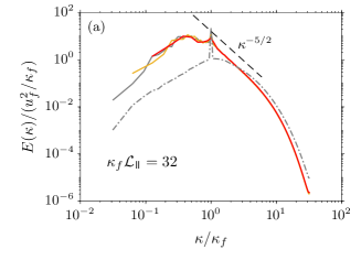
(a)

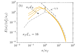
(b)

Figure 8: Three-dimensional spherically averaged energy spectrum for $\kappa_{f}\mathcal{L}_{\mkern 3.0mu\vphantom{\perp}\vrule depth=0.0pt\mkern 2.0mu\vrule depth=0.0pt\mkern 3.0mu}=32$ (a) and $\kappa_{f}\mathcal{L}_{\perp}=16$ (b) with $\mathrm{Ro_{\varepsilon}}\approx 0.06$. Line styles are the same as in Fig. 7, apart from the reference energy spectrum of Fig. 1 with $\kappa_{f}\mathcal{L}_{\perp}=\kappa_{f}\mathcal{L}_{\mkern 3.0mu\vphantom{\perp}\vrule depth=0.0pt\mkern 2.0mu\vrule depth=0.0pt\mkern 3.0mu}=32$ (     ).

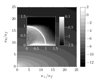
Figure 9: Two-dimensional energy spectrum for $\mathrm{Ro_{\varepsilon}}\approx 0.06$ with $\kappa_{f}\mathcal{L}_{\perp}=\kappa_{f}\mathcal{L}_{\mkern 3.0mu\vphantom{\perp}\vrule depth=0.0pt\mkern 2.0mu\vrule depth=0.0pt\mkern 3.0mu}=32$ (case kf32-a01) at $t=30\,\tau_{f}$. Data is normalized by $(2\pi\kappa_{\perp})\,u_{f}^{2}/\kappa_{f}^{3}$ and plotted in $\log_{10}$. The inset highlights the region around the forcing wavenumber: $\kappa_{\perp}/\kappa_{f}<1.5$ and $\kappa_{\mkern 3.0mu\vphantom{\perp}\vrule depth=0.0pt\mkern 2.0mu\vrule depth=0.0pt\mkern 3.0mu}/\kappa_{f}<1.5$.

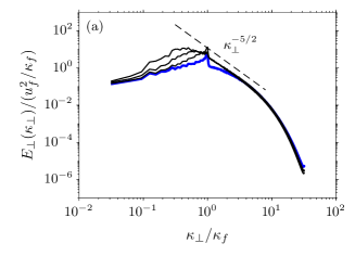
(a)

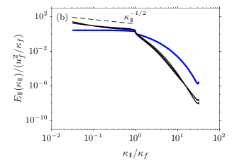
(b)

Figure 10: One-dimensional energy spectra for $\mathrm{Ro_{\varepsilon}}\approx 0.06$ and $\kappa_{f}\mathcal{L}_{\perp}=\kappa_{f}\mathcal{L}_{\mkern 3.0mu\vphantom{\perp}\vrule depth=0.0pt\mkern 2.0mu\vrule depth=0.0pt\mkern 3.0mu}=32$ (case kf32-a01) along directions $\kappa_{\perp}$ (a) and $\kappa_{\mkern 3.0mu\vphantom{\perp}\vrule depth=0.0pt\mkern 2.0mu\vrule depth=0.0pt\mkern 3.0mu}$ (b). Lines represent the time evolution of the energy spectrum: $t=0$ ( ), and $t=10,20$ and $30\,\tau_{f}$ ( ). A reference line for the scaling laws that best agrees with the presented data is also shown (     ).

IV Discussion

This work investigated through direct numerical simulations the effects of domain size and rotation rate on the energy cascade direction of rotating turbulence. The data here presented add substantially to previous works, which, in contrast, focused on smaller and shallower domains ($\kappa_{f}\mathcal{L}_{\mkern 3.0mu\vphantom{\perp}\vrule depth=0.0pt\mkern 2.0mu\vrule depth=0.0pt\mkern 3.0mu}$ and $\kappa_{f}\mathcal{L}_{\perp}$ $<8$ (Smith et al., 1996; Deusebio et al., 2014)). The presented results, therefore, contribute towards a complete picture of the phase diagram, which unveils transition from inverse to forward through a split energy cascade in rotating turbulence.

Our results support $\kappa_{f}\mathcal{L}_{\mkern 3.0mu\vphantom{\perp}\vrule depth=0.0pt\mkern 2.0mu\vrule depth=0.0pt\mkern 3.0mu}$ as the primary control parameter provided that $\mathrm{Ro_{\varepsilon}}$ is constant and $\kappa_{f}\mathcal{L}_{\perp}>4$. In this scenario, transversal finite-size effects of $\kappa_{f}\mathcal{L}_{\perp}$ on the inverse energy transfer $\varepsilon_{inv}$ are negligible for our cases with aspect ratio $A_{r}\geq 1$. For weak rotation with $\mathrm{Ro_{\varepsilon}}\approx 0.31$, transition from a split to a forward cascade was observed at $\kappa_{f}\mathcal{L}_{\mkern 3.0mu\vphantom{\perp}\vrule depth=0.0pt\mkern 2.0mu\vrule depth=0.0pt\mkern 3.0mu}\approx 64$. For the strong rotating case, however, although strongly suppressed, a portion of the injected energy ($\varepsilon_{inv}\approx 0.075\,\varepsilon_{I}$) still cascaded inversely and accumulated at the large scales for $\kappa_{f}\mathcal{L}_{\mkern 3.0mu\vphantom{\perp}\vrule depth=0.0pt\mkern 2.0mu\vrule depth=0.0pt\mkern 3.0mu}=128$.

We attribute the fact that $\varepsilon_{inv}$ does not become exactly zero for $\mathrm{Ro_{\varepsilon}}\approx 0.31$ to two effects. First, the simulations considered in this study are limited to $\mathrm{Re_{\lambda}}\approx 68$. A higher Reynolds number could contribute to a stronger forward cascade, possibly reducing $\varepsilon_{inv}$ to zero. Second, although effects of the geometric non-dimensional parameter $\kappa_{f}\mathcal{L}_{\perp}$ are minor, results hint that larger values of $\kappa_{f}\mathcal{L}_{\perp}$ could also contribute to a reduction of $\varepsilon_{inv}$. In this manner, indefinite increase of $\kappa_{f}\mathcal{L}_{\perp}$ could potentially change the phase diagram in the vicinity of $\varepsilon_{inv}/\varepsilon_{I}=0$, and could cause regime transition to be sharp rather than smooth. The recent study of Benavides and Alexakis (2017) has shown that a continuous increase of horizontal domain dimensions shifts the transition behavior for thin layer turbulence from smooth to critical. We hope that further studies will help to fill the parameter space for higher Reynolds numbers and even longer domain sizes.

For $\mathrm{Ro_{\varepsilon}}\approx 0.06$, we agree with Deusebio et al. (2014) and believe that a continuous increase of $\kappa_{f}\mathcal{L}_{\mkern 3.0mu\vphantom{\perp}\vrule depth=0.0pt\mkern 2.0mu\vrule depth=0.0pt\mkern 3.0mu}$ would result in transition to a forward energy cascade. Nevertheless, results for the weak case suggest a slow-paced transition and significantly larger values for $\kappa_{f}\mathcal{L}_{\mkern 3.0mu\vphantom{\perp}\vrule depth=0.0pt\mkern 2.0mu\vrule depth=0.0pt\mkern 3.0mu}$ might be required. Interestingly, the transition of $\varepsilon_{inv}$ in terms of $\kappa_{f}\mathcal{L}_{\mkern 3.0mu\vphantom{\perp}\vrule depth=0.0pt\mkern 2.0mu\vrule depth=0.0pt\mkern 3.0mu}$ resembles a logistic function, similar to what has been found for regime transitions in thin layer turbulence (Benavides and Alexakis, 2017).

In search of a criteria for transition between a forward and a split cascade system, we made an attempt to express $\varepsilon_{inv}/\varepsilon_{I}$ for all parameter points as a function of $\mathrm{Ro_{\varepsilon}}\kappa_{f}\mathcal{L}_{\mkern 3.0mu\vphantom{\perp}\vrule depth=0.0pt\mkern 2.0mu\vrule depth=0.0pt\mkern 3.0mu}$. As the different curves do not overlap, we believe that a criteria for transition should stem from a more general match of timescales. A criteria such as $\mathrm{Ro_{\varepsilon}}\kappa_{f}\mathcal{L}_{\mkern 3.0mu\vphantom{\perp}\vrule depth=0.0pt\mkern 2.0mu\vrule depth=0.0pt\mkern 3.0mu}=C$, can be obtained by requiring the slowest inertial wave frequency $1/\tau_{w}=2\Omega/\kappa_{f}\mathcal{L}_{\mkern 3.0mu\vphantom{\perp}\vrule depth=0.0pt\mkern 2.0mu\vrule depth=0.0pt\mkern 3.0mu}$ and the eddy turnover frequency $u_{f}\kappa_{f}$ at the forcing scale to be of same order (Alexakis and Biferale, 2018; Seshasayanan and Alexakis, 2018). Alternatively, we can frame the problem within the idea that rotation alters the spectral transfer time $\tau_{s}$ at which energy is transferred to smaller scales. Thus, it follows that $\varepsilon_{\nu}\sim u_{\ell}^{2}/\tau_{s}$, with $u_{\ell}$ a velocity scale characteristic of eddies of size $\ell$, and $\tau_{s}\sim\tau_{nl}^{2}/\tau_{3}$ (Kraichnan, 1965; Zhou, 1995; Galtier, 2003). Here, $\tau_{nl}\sim\ell/u_{\ell}$ is the nonlinear timescale and $\tau_{3}$ is the relaxation time of triple velocity correlations. The relaxation time in isotropic turbulence simplifies to $\tau_{nl}$ to recover the dissipation law, i.e. $\varepsilon_{\nu}\sim u_{\ell}^{3}/\ell$.

Now the condition $\mathrm{Ro_{\varepsilon}}\kappa_{f}\mathcal{L}_{\mkern 3.0mu\vphantom{\perp}\vrule depth=0.0pt\mkern 2.0mu\vrule depth=0.0pt\mkern 3.0mu}=C$ can be obtained by requiring $\varepsilon_{\nu}=\varepsilon_{I}$, and assuming $u\sim u_{f}$, $\tau_{nl}\sim\tau_{f}$ and $\tau_{3}\sim\tau_{w}$. So, $\mathrm{Ro_{\varepsilon}}\kappa_{f}\mathcal{L}_{\mkern 3.0mu\vphantom{\perp}\vrule depth=0.0pt\mkern 2.0mu\vrule depth=0.0pt\mkern 3.0mu}=C$ is equivalent to state that in the presence of rotation the nonlinear timescale remains of the order of $\tau_{f}$, and that the relaxation timescale $\tau_{3}$ is given by the inverse of the slowest inertial wave frequency, i.e $\tau_{3}\sim\tau_{w}$. A generalization of the previous reasoning would be to consider a $\tau_{nl}$ obtained from a measured velocity quantity, like the r.m.s velocity, and the lengthscale $\ell$ possibly as $\ell_{\perp}$, as the triadic interactions are expected to be depleted in the direction parallel to the rotation axis (Nazarenko and Schekochihin, 2011). The relaxation time $\tau_{3}$ could be sought as a function of both $\tau_{f}$ and $\tau_{\Omega}$. In this manner, more general criteria like $\mathrm{Ro_{\varepsilon}}^{a}(\kappa_{f}\mathcal{L}_{\mkern 3.0mu\vphantom{\perp}\vrule depth=0.0pt\mkern 2.0mu\vrule depth=0.0pt\mkern 3.0mu})^{b}=C$ arise, where $a$ and $b$ are yet undetermined exponents.

Results for scaling laws of the energy spectrum are here not conclusive, and there is no clear sign of an inertial range over several decades. This is plausible since our initial and isotropic field with $\mathrm{Re_{\lambda}}\approx 68$ does not contain a clear inertial range. In spite of that, the narrow wavenumber region after $\kappa_{\perp}=\kappa_{f}$ develops and approaches best a $\kappa_{\perp}^{-5/2}$ scaling law. Our results also show that, the $\kappa_{\perp}^{-5/2}$ and $\kappa_{\mkern 3.0mu\vphantom{\perp}\vrule depth=0.0pt\mkern 2.0mu\vrule depth=0.0pt\mkern 3.0mu}^{-1/2}$ scalings appear at different wavenumber ranges, and that the $\kappa^{-5/2}$ scaling prevails in the 3D energy spectrum, see Fig. 8.

References

- Frisch (1995) U. Frisch, Turbulence: The Legacy of A. N. Kolmogorov. Cambridge (Cambridge University Press, 1995).
- Alexakis and Biferale (2018) A. Alexakis and L. Biferale, Physics Reports (2018), 10.1016/j.physrep.2018.08.001.
- Boffetta and Ecke (2012) G. Boffetta and R. E. Ecke, Annual Review of Fluid Mechanics 44, 427 (2012).
- Greenspan (1968) H. P. Greenspan, The Theory of Rotating Fluids (Cambridge University Press, 1968).
- Godeferd et al. (2015) F. S. Godeferd, F. Ed, and E. Moisy, Applied Mechanics Reviews 67, 030802 (2015).
- Waleffe (1993) F. Waleffe, Physics of Fluids 677, 667 (1993).
- Cambon et al. (1997) C. Cambon, N. N. Mansour, and F. S. Godeferd, Journal of Fluid Mechanics 337, 337 (1997).
- Smith and Waleffe (1999) L. Smith and F. Waleffe, Physics of Fluids 11, 1608 (1999).
- Buzzicotti et al. (2018) M. Buzzicotti, H. Aluie, L. Biferale, and M. Linkmann, Physical Review Fluids 3, 034802 (2018), 1711.07054 .
- Yeung and Zhou (1998) P. K. Yeung and Y. Zhou, Physics of Fluids 10, 2895 (1998).
- Mininni et al. (2009) P. D. Mininni, A. Alexakis, and A. Pouquet, Physics of Fluids 21, 015108 (2009).
- Moisy et al. (2011) F. Moisy, C. Morize, M. Rabaud, and J. Sommeria, Journal of Fluid Mechanics 666, 5 (2011).
- Mininni et al. (2012) P. D. Mininni, D. Rosenberg, and A. Pouquet, Journal of Fluid Mechanics 699, 263 (2012).
- Delache et al. (2014) A. Delache, C. Cambon, and F. Godeferd, Physics of Fluids 26, 025104 (2014).
- Linkmann and Dallas (2017) M. Linkmann and V. Dallas, Physical Review Fluids 2, 1 (2017), 1702.04787 .
- Moffatt (2014) H. K. Moffatt, Journal of Fluid Mechanics 741, R3 (2014).
- Galtier (2003) S. Galtier, Physical Review E 68, 015301 (2003).
- Nazarenko (2011) S. Nazarenko, Wave Turbulence, Lecture Notes in Physics (Springer Berlin Heidelberg, 2011).
- Smith et al. (1996) L. M. Smith, J. R. Chasnov, and F. Waleffe, Physical Review Letters 77, 2467 (1996).
- Celani et al. (2010) A. Celani, S. Musacchio, and D. Vincenzi, Physical Review Letters 104, 1 (2010).
- Benavides and Alexakis (2017) S. J. Benavides and A. Alexakis, Journal of Fluid Mechanics 822, 364 (2017).
- Deusebio et al. (2014) E. Deusebio, G. Boffetta, E. Lindborg, and S. Musacchio, Physical Review E 90, 023005 (2014).
- Seshasayanan and Alexakis (2018) K. Seshasayanan and A. Alexakis, Journal of Fluid Mechanics 841, 434 (2018).
- Orszag (1971) S. A. Orszag, Journal of Fluid Mechanics 49, 75 (1971).
- Pekurovsky (2012) D. Pekurovsky, SIAM Journal on Scientific Computing 34, C192 (2012).
- Rogallo (1977) R. S. Rogallo, NASA STI/Recon Technical Report N 78, 13367 (1977).
- Morinishi et al. (2001) Y. Morinishi, K. Nakabayashi, and S. Q. Ren, International Journal of Heat and Fluid Flow 22, 30 (2001).
- Alvelius (1999) K. Alvelius, Physics of Fluids 11, 1880 (1999).
- Dallas et al. (2015) V. Dallas, S. Fauve, and A. Alexakis, Physical Review Letters 115, 204501 (2015), 1507.01874 .
- Kraichnan (1965) R. H. Kraichnan, Physics of Fluids 8, 1385 (1965).
- Zhou (1995) Y. Zhou, Physics of Fluids 7, 2092 (1995).
- Nazarenko and Schekochihin (2011) S. V. Nazarenko and A. A. Schekochihin, Journal of Fluid Mechanics 677, 134 (2011).