Planck 2018 and Brane Inflation Revisited

Abstract

We revisit phenomenological as well as string-theoretical aspects of D-brane inflation cosmological models. Phenomenologically these models stand out on par with $\alpha$-attractors, as models with Planck-compatible values of $n_{s}$, moving down to the sweet spot in the data with decreasing value of $r$. On the formal side we present a new supersymmetric version of these models in the context of de Sitter supergravity with a nilpotent multiplet and volume modulus stabilization. The geometry of the nilpotent multiplet is evaluated in the framework of string theory.

1 Introduction

D-brane inflation models have two aspects, a phenomenological and a string-theoretical. Both became very interesting after the investigation of inflationary models in the Planck 2018 data release Akrami:2018odb . The Planck 2018 $n_{s}$ - $r$ plane is shown in Fig. 1. The dark (light) blue regions describe the $1\sigma$ ($2\sigma$) confidence level for the CMB related data obtained by Planck 2018 and Bicep/Keck2014, additionally including the baryon oscillations (BAO) data. Meanwhile the comparison of predictions of inflationary models with the data in Akrami:2018odb was based on the CMB related data only, excluding BAO. The corresponding 1$\sigma$ and 2$\sigma$ regions are shown in red in Fig. 1.

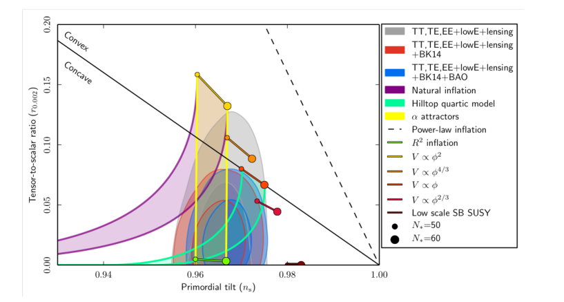
Figure 1: The results of the Planck 2018 data release. The two yellow lines correspond to $\alpha$-attractors with $n_{s}\approx 1-{2\over N_{e}}$, with the number of e-foldings $N_{e}=50$ and $N_{e}=60$.

The main part of the left hand side of the $1\sigma$ region in this plane is described by the simplest $\alpha$-attractor model Kallosh:2013yoa , with the predictions bounded by the two yellow lines corresponding to the $\alpha$-attractor prediction

$$n_{s}=1-{2\over N_{e}}\,$$ (1)

with the number of e-foldings $N_{e}=50$ and $N_{e}=60$. The lower part of the $\alpha$-attractor yellow band covers also the predictions of the Starobinsky model  Starobinsky:1980te , the GL supergravity model Goncharov:1985yu , and the Higgs inflation model Salopek:1988qh ; Bezrukov:2007ep . The values of $n_{s}$ and $r$ for $\alpha$-attractor models were shown in Kallosh:2013yoa and Carrasco:2015pla , see Fig. 3 here. Special cases with $\alpha=1$ correspond to Starobinsky, Higgs and conformal inflation Kallosh:2013hoa , $\alpha=1/9$ corresponds to the GL model Goncharov:1985yu , $\alpha=2,1/2$ correspond to fibre inflation Cicoli:2008gp ; Kallosh:2017wku . Models with $3\alpha=7,6,5,4,3,2,1$ originate from theories with maximal supersymmetry Ferrara:2016fwe ; Kallosh:2017ced .

2

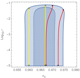
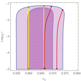
Figure 2: Comparison of predictions of $\alpha$-attractors and of the D-brane inflationary model with $V\sim 1-\Big{(}{m\over\phi}\Big{)}^{4}$ within the $2\sigma$ area of the Planck 2018 results for $n_{s}$ and $r$. On the left panel, the dark (light) blue area is the Planck 2018 $1\sigma$ ($2\sigma$) region, with an account taken of the CMB-related data. The right panel represents the Planck 2018 results based on the CMB related data only, without BAO. Two yellow lines on both panels are for the quadratic T-model of $\alpha$-attractors at $N_{e}=50$ and $N_{e}=60$. Two red lines are for the simplest D-brane inflation model $V=1-\Big{(}{m\over\phi}\Big{)}^{4}$.

As one can see from Akrami:2018odb , the two yellow lines corresponding to $\alpha$-attractors cover the left hand side of the $1\sigma$ dark blue (and dark red) areas in Fig. 1. However, the Planck 2018 analysis of inflationary models presented in Table 5 in Akrami:2018odb reveals yet another class of models, which may match the observations equally well, in a complementary way. It is a class of D-brane inflation models with the potential proportional to $1-\Big{(}{m\over\phi}\Big{)}^{4}+\cdots$, studied in Appendix C of the KKLMMT paper Kachru:2003sx . Predictions of such models cover the right hand side of the $1\sigma$ dark blue (and dark red) areas in Fig. 1.

As an example, let us simultaneously plot the predictions of $\alpha$-attractors and of the simplest D-brane inflationary model with $V\sim 1-\Big{(}{m\over\phi}\Big{)}^{4}$ in figures representing the Planck 2018 data for $r$ on $\log_{10}r$ scale, which is more suitable for illustration of the predictions of the models in the limit of small $r$, where both of these classes of models exhibit attractor behavior, see Fig. 2. As one can see from this figure, the combination of the simplest $\alpha$-attractor model and the simplest D-brane inflation model almost completely cover the $1\sigma$ dark blue (dark purple) area of the Planck 2018 data.

The reason why the predictions of $\alpha$-attractors and of the simplest D-brane inflation match each other in Fig. 2 so perfectly is very simple. According to the investigation in Appendix C of Kachru:2003sx , the value of $n_{s}$ in the D-brane inflationary model with $V\sim 1-\Big{(}{m\over\phi}\Big{)}^{4}$ in the small $m$ (small $r$) limit is given by

$$n_{s}=1-{5\over 3N_{e}}\ .$$ (2)

The cosmological evolution in these models was studied in detail in Lorenz:2007ze and in Sect. 5.19 of Martin:2013tda , see Figs. 159-166 there.

Magically, $n_{s}$ for $\alpha$-attractors shown by the right yellow line corresponding to $N_{e}=60$ in Fig. 2 exactly coincides with $n_{s}$ for the simplest D-brane inflation models for the left red line with $N_{e}=50$:

$$n_{s}=1-{2\over 60}=1-{5\over 3\times 50}=1-{1\over 30}=0.967\ .$$ (3)

This explains why $\alpha$-attractors and D-brane inflation match Planck results so well in Fig. 2, and why both models provide a very good match to the Planck 2018 result $n_{s}=0.9649\pm 0.0042$ Akrami:2018odb .

Of course, one should remember that exact predictions of these models depend on details of the models, mechanism of reheating, etc., and the position of the $1\sigma$ region for Planck 2018 depends on the data set (e.g. with or without BAO). Nevertheless the perfect match shown in Fig. 2 is quite striking.

Note, that the predictions of $\alpha$-attractors also allow some variability, converging to (1) in the limit of large $N_{e}$, and small $\alpha$, which corresponds to small $r$, see Fig. 3.

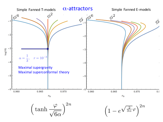
Figure 3: $\alpha$-attractor models in $n_{s}$ - $r$ plane at $N_{e}=60$.

Thus, phenomenologically D-brane inflation model after Planck 2018 has acquired a new significance, even independent of its string theory origin. But we will show here that a new progress can be made with regard to string theory implementation of the phenomenologically attractive versions of D-brane inflation model.

The string theory origin of D-brane inflation model is often attributed to KKLMMT model Kachru:2003sx , where D3-brane-$\overline{\rm D3}$-brane interaction was studied in the context of the volume modulus stabilization. Earlier proposals for D-brane inflation relevant to our current discussion were made in Dvali:2001fw ; Burgess:2001fx ; GarciaBellido:2001ky . The inflationary potentials corresponding to Dp-brane-$\overline{\rm Dp}$-brane interaction were proposed in the form

$$V_{BI}=V_{0}\Big{(}1-\Big{(}{m\over\phi}\Big{)}^{7-p}+\cdots\Big{)}\,,\qquad V_{KKLTI}=V_{0}\Big{(}1+\Big{(}{m\over\phi}\Big{)}^{7-p}\Big{)}^{-1}.$$ (4)

In Martin:2013tda a detailed cosmological analysis of both potentials was performed, with emphasis on the cases $p=3$ and $p=5$, i.e. for inverse quartic and quadratic potentials. The first potential in (4) was called BI (Brane Inflation), the second one was called KKLTI (KKLT Inflation).

The earlier proposals in Dvali:2001fw ; Burgess:2001fx ; GarciaBellido:2001ky were made without addressing the volume stabilization issue. A consistent cosmological evolution of Dp-branes in string theory with the fundamental ten-dimensional geometry can be interpreted as an evolution in the four-dimensional Einstein equations under condition that the six-dimensional internal space has a constant volume, not a runaway behavior which destroys the consistency of the four-dimensional cosmology.

In Kachru:2003sx D3-brane-$\overline{\rm D3}$-brane interaction was studied simultaneously with the volume stabilization. The concrete example in string theory was based on strong warping, which is dual to an almost conformal four-dimensional field theory. Therefore the scalar field describing the motion of the brane was conformally coupled to gravity. This was consistent with the choice of the Kähler  potential and the KKLT superpotential in the form

$$K=-3\log(T+\bar{T}-\Phi\bar{\Phi})\,,\qquad W=W_{0}+A(\Phi)e^{-T}.$$ (5)

However, it is well known that it is difficult to achieve inflation in the theories with a conformally coupled inflaton. This was one of the the main reasons to consider a generalized KKLT superpotential (5) where the dependence on the distance between branes $\Phi$ was included in $A(\Phi)$. A specific explicit model of inflation which followed from (5) was presented in Baumann:2007ah . The corresponding potential, an inflection point potential, has $n_{s}\approx 0.93$, which is ruled out by the data, see for example Fig. 1. More about the derivation of this model can be found in a review paper on string cosmology Baumann:2014nda .

The reason for us to revisit the KKLMMT paper Kachru:2003sx after Planck 2018 is that, in addition and independently of an example of a particular form of the Kähler  potential and superpotential (5), Ref. Kachru:2003sx provided a basis for other, more general approaches to string cosmology. It can be used at present in a form which is in fact supported by the latest data, using in particular equation (2) for the tilt of the spectrum as derived in Appendix C of Kachru:2003sx . We will therefore start with phenomenological properties of D-brane inflation models following Kachru:2003sx ; Lorenz:2007ze ; Martin:2013tda , and then we will discuss a possibility to implement such models in supergravity and string theory.

2 Phenomenological D-brane inflation models

2.1 KKLMMT scenario and inverse quartic and quadratic models

A short preview of the phenomenology of the simplest D-brane inflationary models is given in Figure 2. In this section we will study a broad class of phenomenological models of D-brane inflation in greater detail. As in Encyclopedia Inflationaris Martin:2013tda , we will call the corresponding potentials either BI (Brane Inflation) for a Coulomb-type interaction, or KKLTI (for KKLT Inflation) when the potential takes a form of the inverse harmonic function. The case of the inverse quadratic Coulomb-type interaction is

$${}^{2}V_{BI}=V_{0}\Big{[}1-\Big{(}{m\over\phi}\Big{)}^{2}+\cdots\Big{]}\,,$$ (6)

whereas the potential in a form of the inverse harmonic function is

$${}^{2}V_{KKLTI}=V_{0}\Big{[}1+\Big{(}{m\over\phi}\Big{)}^{2}\Big{]}^{-1}=V_{0}\Big{[}{\phi^{2}\over m^{2}+\phi^{2}}\Big{]}\ .$$ (7)

At small ${m\over\phi}$ the ‘exact’ non-singular at $\phi=0$ potential $V_{KKLTI}$ takes the form of $V_{BI}$. At very large values of $m$ the potential tends to a quadratic one, in the area where $\phi\ll m$,

$${}^{2}V_{KKLTI}\Rightarrow{V_{0}\over m^{2}}\phi^{2}.$$ (8)

In the limit $m\gg 1$, predictions of this model coincide with the predictions of the simplest chaotic inflation model $V\sim\phi^{2}$, which is ruled out. However, as we will see soon, in the case $m\lesssim 1$ this model provides a good fit to Planck 2018 data, see Fig. 4.

The case of the inverse quartic Coulomb-type interaction is

$${}^{4}V_{BI}=V_{0}\Big{[}1-\Big{(}{m\over\phi}\Big{)}^{4}+\cdots\Big{]}\,,$$ (9)

whereas the potential in a form of the inverse harmonic function is

$${}^{4}V_{KKLTI}=V_{0}\Big{[}1+\Big{(}{m\over\phi}\Big{)}^{4}\Big{]}^{-1}=V_{0}\Big{[}{\phi^{4}\over m^{4}+\phi^{4}}\Big{]}\ .$$ (10)

Here again, at small ${m\over\phi}$ the ‘exact’ non-singular at $\phi=0$ potential $V_{KKLTI}$ takes the form of $V_{BI}$. At very large values of $m$ the potential tends to a quartic one, in the area where $\phi\ll m$,

$${}^{4}V_{KKLTI}\Rightarrow{V_{0}\over m^{4}}\phi^{4}.$$ (11)

The $\alpha$-attractor models have

$$n_{s}\approx 1-{2\over N_{e}}.$$ (12)

For Dp-brane-$\overline{\rm Dp}$-brane inflation models with $V=A-{B\over\phi^{7-p}}$, the general formula for small $r$ is

$$n_{s}\approx 1-{2(8-p)\over(9-p)N_{e}}.$$ (13)

This was also given in Burgess:2001fx and in Martin:2013tda in slightly different notation. For example in Martin:2013tda the formula is in terms of $k=7-p$ and is given as $n_{s}\approx 1-{2(k+1)\over(k+2)N_{e}}$. Note that for the polynomial potentials $\phi^{2n}$

$$n_{s}\approx 1-{n+1\over N_{e}}\ .$$ (14)

This means that the brane inflation spectral index $n_{s}$ at small $r$ coincides with $n_{s}$ of inflation in a theory with a polynomial potential $\phi^{2n}$ with

$$n\,\Leftrightarrow\,{7-p\over 9-p}\ .$$ (15)

The quartic brane inflation for D3-$\overline{\rm D3}$ model at small $r$ has the same $n_{s}$ Kachru:2003sx as the one for $\phi^{4/3}$:

$$n_{s}=1-{5\over 3N_{e}}\qquad\,\Leftrightarrow\,\qquad n_{s}(\phi^{4/3})\approx 1-{{2\over 3}+1\over N_{e}}\ ,$$ (16)

in agreement with with the general equation (13) for $p=3$.

The quadratic brane inflation model, with D5-$\overline{\rm D5}$ potential, at small $r$ has the same $n_{s}$ GarciaBellido:2001ky as inflation in a theory with a linear potential $\phi$,

$$n_{s}\approx 1-{3\over 2N_{e}}\qquad\,\Leftrightarrow\,\qquad n_{s}(\phi)\approx 1-{{1\over 2}+1\over N_{e}}\ ,$$ (17)

in agreement with the general equation (13) for $p=5$.

On the left side in Fig. 4 we have an $\alpha$-attractor band which starts at $\phi^{2}$ and moves down in a straight line. Next is the inverse quartic brane inflation model which at small $r$ is in the position corresponding to $\phi^{4/3}$, both for BI and KKLTI models, and continues straight. The inverse quadratic brane inflation at small at the right panel in Fig. 4 at small $r$ is in a position corresponding to $\phi$, both for BI and KKLTI models, and continues straight. These three models pretty much cover all admissible area in the $n_{s}-r$ plane below $r<10^{-2}$.

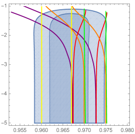
Figure 4: Predictions of $\alpha$-attractors and KKLTI/BI models. The dark (light) blue area is the Planck 2018 $1\sigma$ ($2\sigma$) region, with an account taken of TT, TE, EE + lowE + lensing + BK14+BAO Akrami:2018odb . Two yellow lines on the left panel are for the quadratic T-model of $\alpha$-attractors at $N_{e}=50$ and $N_{e}=60$. Two purple lines are for the quartic KKLTI model, two red lines are for the quartic BI model. As one can see, the combination of the simplest $\alpha$-attractor model and the quartic KKLTI/BI model (including the models interpolating between KKLTI and BI) completely cover the $1\sigma$ area of the Planck 2018 data. Two orange lines show the predictions of the quadratic KKLTI model, and two green lines are for the quadratic BI model.

To understand the reason of similarity between predictions of $\alpha$-attractors and D-brane inflation, we show in Fig. 5 two potentials. One of them is the potential of the $\alpha$-attractor model with $V=\tanh^{4}{\phi\over\sqrt{6\alpha}}$ with $\alpha=1/6$. The second one is of the inverse quartic D-brane inflation type, $V={\phi^{4}\over\phi^{4}+m^{4}}$ for $m=1$. This figure shows that in both cases we have plateau potentials at large fields, and for some choice of parameters (e.g. for $\alpha=1/9$ and $m=1$) one can even make these potentials look even more similar, even though predictions of these models for $n_{s}$ continue to be slightly different.

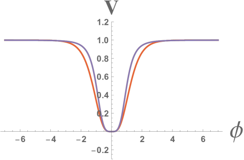
Figure 5: The red line shows the quartic $\alpha$-attractor potential $V=\tanh^{4}{\phi\over\sqrt{6\alpha}}$ with $\alpha=1/6$. The dark blue line shows the KKLTI potential $V={\phi^{4}\over\phi^{4}+m^{4}}$ for $m=1$. In both cases we have plateau potentials at large $\phi$. For some choices of parameters (e.g. for $\alpha=1/9$ and $m=1$) these potentials almost coincide, which explains similarity of predictions of these models.

The value of $r$ for $\alpha$-attractors depends on $\alpha$,

$$r\approx{12\alpha\over N_{e}^{2}}\,.$$ (18)

Meanwhile in brane inflation models the value of $r$ depends on $m$. In quartic case, using Kachru:2003sx for $m\lesssim 1$ one finds

$$r\approx{4m^{{4\over 3}}\over(3N_{e})^{5\over 3}}\ .$$ (19)

In particular, for $m=1$, $N_{e}=50$ we find $r\sim 10^{{-3}}$. Using eq. (5.332) of Martin:2013tda , we find a more general expression for $r$ for $V=1-\left(\frac{m}{\phi}\right)^{k}$,

$$r\approx 8k^{2}\left(k(k+2)N_{e}\right)^{-\frac{2k+2}{k+2}}m^{\frac{2k}{k+2}}.$$ (20)

For an inverse quadratic potential with $k=2$ we find

$$r\approx{\sqrt{2}\,m\over N_{e}^{3\over 2}}\ .$$ (21)

In particular, for $m=1$, $N_{e}=50$ we find $r\sim 4\times 10^{-3}$.

It is instructive to compare these results with the ones presented in Fig. 4. One can see that with the decrease of $r$ the results for $n_{s}$ in the BI and KKLTI models converge to each other at the values of $r$ approximately corresponding to $m\sim 1$, just as one could expect by comparing to each other the potentials of these models.

Thus here we have presented our analysis of quartic and quadratic BI and KKLTI models inside $2\sigma$ region of Planck 2018. As we see, the combination of these models covers the main part of the $2\sigma$ area in the Planck 2018 data in Fig. 4. This is explained by the similarity of potentials of these models illustrated by Fig. 5. Our results are compatible with the ones found in Martin:2013tda .

2.2 Inverse linear case with D6-$\overline{\rm D6}$ potential

In the previous discussion we concentrated on investigation of inverse quadratic and inverse quartic mode, as in the Planck 2018 analysis in Akrami:2018odb . Both cases are associated with type IIB string theory, where moduli stabilization was viewed as possible due to KKLT and LVS constructions. However, there was a progress recently with regard to an uplifting role of the $\overline{\rm D6}$ brane in Kallosh:2018nrk and de Sitter vacua in type IIA string theory in Blaback:2018hdo .

Therefore we would like to add here an example of D6-$\overline{\rm D6}$ potential using the general equations above to find out the phenomenology of these models. This is the case of $k=7-p=1$,

$${}^{1}V_{BI}=V_{0}\Big{[}1-\Big{(}{m\over|\phi|}\Big{)}+\cdots\Big{]}\,,$$ (22)

$${}^{1}V_{KKLTI}=V_{0}\Big{[}1+\Big{(}{m\over|\phi|}\Big{)}\Big{]}^{-1}=V_{0}\Big{[}{|\phi|\over m+|\phi|}\Big{]}\ .$$ (23)

Note that the variable $\phi$ is not a coordinate, but a distance in the moduli space, $\phi=|\phi|\times e^{{i\theta}}$, which is why the potentials depend on $|\phi|$.

At large $m$, the predictions of the ${}^{1}V_{KKLTI}$ model converge to the predictions of the theory with a simple linear potential $V\sim\phi$. However, at small $m$ it predicts the same value of $n_{s}$ as the theory with $V\sim\phi^{2/3}$.

At large $N_{e}$ and small $r$ (for $m<1$), the predictions are

$$n_{s}\approx 1-{4\over 3N_{e}}\ ,\qquad r\approx{8m^{2\over 3}\over\left(3N_{e}\right)^{{3\over 4}}}.$$ (24)

For $N_{e}=50$ this gives $n_{s}\approx 0.973$, which is within the $2\sigma$ Planck area for small $r$.

3 D-brane Dynamics

3.1 String theory analysis

To understand the D-brane dynamics in string theory in application to inflation it is useful to consider the original Polchinski’s computation of the energy between two parallel Dirichlet p-branes at the distance $Y$ from each other Polchinski:1996na ; Bachas:1998rg , see Fig. 6. In eq. (90) in Polchinski:1996na there is an answer for

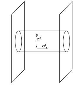
Figure 6: Exchange of a closed string between two D-branes. Equivalently, a vacuum loop of an open string with one end on each D-brane.

two D-branes. Here we present it both for two D-branes, with the negative contribution from the open string R sector, as well as for one D-brane-anti-D-brane with the positive contribution from the open string R sector

$$A=\pm{\cal A}_{\rm R}+{\cal A}_{\rm NS}=2V_{p+1}\int{dt\over 2t}\,(8\pi^{2}\alpha^{\prime}t)^{-{p+1\over 2}}e^{-t{Y^{2}\over 2\pi\alpha^{\prime}}}\,\frac{\mp f_{2}(q)^{8}+f_{3}(q)^{8}-f_{4}(q)^{8}}{2f_{1}^{8}(q)},$$ (25)

where $q=e^{-\pi t}$ and all functions $f_{i}(q)$ are defined in eq. (49) in Polchinski:1996na and $t$ is world sheet modulus. This takes into account that the world-sheet fermions that are periodic around the cylinder correspond to R-R exchange, while the ones which are anti-periodic come from NS-NS exchange.

These three terms for two Dp-branes sum to zero by the ‘abstruse identity,’ since in this case the open string spectrum is supersymmetric. But in case of D-brane-anti-D-brane, when R-sector has a different sign, they sum up since

$${\cal A}_{\rm NS}\ =\ -{\cal A}_{\rm R}.$$ (26)

Thus for two D-branes

$$A_{Dp/Dp}={\cal A}_{\rm R}+{\cal A}_{\rm NS} = 2V_{p+1}\int{dt\over 2t}\,(8\pi^{2}\alpha^{\prime}t)^{-{p+1\over 2}}e^{-t{Y^{2}\over 2\pi\alpha^{\prime}}}$$ (27)

$$\qquad\qquad\qquad\qquad\qquad\frac{-f_{2}(q)^{8}+f_{3}(q)^{8}-f_{4}(q)^{8}}{2f_{1}^{8}(q)}=0.$$

In terms of the closed string exchange, this reflects the fact that D-branes are BPS states, the net forces from NS-NS and R-R exchanges canceling. For D-brane-anti-D-brane

$$A_{Dp/\bar{D}p}=-{\cal A}_{\rm R}+{\cal A}_{\rm NS}=2{\cal A}_{\rm NS} = 2V_{p+1}\int{dt\over 2t}\,(8\pi^{2}\alpha^{\prime}t)^{-{p+1\over 2}}e^{-t{Y^{2}\over 2\pi\alpha^{\prime}}}\,\frac{f_{2}(q)^{8}}{f_{1}^{8}(q)}.$$ (28)

We are interested in the limit $t\rightarrow 0$ which is dominated by the lowest lying modes in the closed string spectrum. In such case

$$A_{Dp/\bar{D}p}^{t\rightarrow 0} \sim V_{p+1}\int{dt\over t}(2\pi t)^{-(p+1)/2}(t/2\pi\alpha^{\prime})^{4}e^{-t{Y^{2}\over 8\pi^{2}\alpha^{\prime 2}}}$$ (30)

$$= V_{p+1}4\pi(4\pi^{2}\alpha^{\prime})^{3-p}G_{9-p}(Y^{2}).$$

Here $G_{9-p}(Y^{2})$ is a massless propagator in the Euclidean $9-p$ dimension. The corresponding equation is

$$\Delta^{2}_{9-p}G_{9-p}(Y^{2})=C\delta^{9-p}(Y)\,,\qquad G_{9-p}(Y^{2})\sim\Big{[}c_{1}+{c_{2}\over Y^{7-p}}\Big{]}^{-1}.$$ (31)

For example, for D3 case it is $\Delta^{2}_{6}G_{6}(Y^{2})=C\delta^{6}(Y)$ and

$$A_{D3/\bar{D}3}^{t\rightarrow 0} \sim \Big{(}c_{2}+{c_{1}\over Y^{4}}\Big{)}^{-1}\sim b_{2}-{b_{1}\over Y^{4}}+\cdots.$$ (32)

Thus for two D-branes the net force between Ramond-Ramond repulsion and gravitational plus dilaton attraction cancels. For D-brane-anti-D-brane the force between Ramond-Ramond attraction and gravitational plus dilaton attraction doubles.

At large distances $Y$ one can use an approximated expression for the cylinder amplitude at (30). At short distances $b_{1}-{b_{2}\over Y^{4}}$ blows up, but it means that our approximation where only low lying string states are taken into account is not valid and the full tower of string states contributes as shown in eq. (28).

From the perspective of string theory computation with the result in (28) it would be confusing to use the concept of the brane-anti-brane annihilation. D-branes and anti-D-branes are not particles with the opposite charge which annihilate and disappear. When the distance between them is small one should not use the approximation $t\rightarrow 0$ which allows to use the harmonic function in eq. (30) and the corresponding potential energy of the brane-anti-brane system. It is the difference between particles and strings which becomes essential at small distances which has to be taken into account in attempts to provide an interpretation of this physical system.

In application to cosmology we will be interested in both potentials in eq. (32). But we will be particularly interested in the region where the difference between these two is not significant.

3.2 On ${\rm D3}/\overline{\rm D3}$ potential in the space-time picture

Now we follow the strategy in KKLMMT paper Kachru:2003sx where in Sec. 2 and in Appendix B a computation of the D3/$\overline{\rm D3}$ potential in warped geometries is proposed. This is also related to a discussion above were we followed Polchinski:1996na ; Bachas:1998rg in their computation of the cylinder diagram directly in string theory. It is also useful to follow Lorenz:2007ze where the same procedure is explained conveniently, not necessarily requiring a warped 5d geometry. The review of inflation in string theory in Baumann:2014nda is also helpful here. Note that here we assume that we already have a space-time picture. This means that the full string theory computation in (28) is already approximated by the case where $t\rightarrow 0$ limit is taken. But we will see a different way how the harmonic function in the $9-p=6$ Euclidean space shows up and defines the potential of the D3/$\overline{\rm D3}$ system.

D3-brane is perturbing the background and we calculate the resulting energy of the $\overline{\rm D3}$-brane in this perturbed geometry. This gives the same answer for the potential energy of the brane-anti-brane pair. We start with 10d geometry

$$ds^{2}=h^{-1/2}ds_{4}^{2}+h^{-1/2}ds_{4}^{2}\,,\qquad F_{5}=\partial_{r}h^{-1}\ .$$ (33)

In case that the moving D3-brane is at a position $r_{1}$ at a radial location in the six-dimensional space and the $\overline{\rm D3}$-brane is at a fixed position $r$ the corresponding harmonic function in the six-dimensional space is given in KKLMMT as

$$h+\delta h=R^{4}\Big{(}{1\over r^{4}}+{1\over N}{1\over r_{1}^{4}}\Big{)}.$$ (34)

Here $R$ is a characteristic length scale of the $AdS_{5}$ geometry, and $N$ is the five-form charge. This expression is valid for strongly warped geometries. In Lorenz:2007ze a general form of a harmonic function is used, namely for a position of the moving brane $\phi$, which has a canonical kinetic term following from the D-brane action

$$\tilde{h}(\phi)=c_{2}+{c_{1}\over\phi^{4}}\ ,$$ (35)

where $c_{1},c_{2}$ are some constants. This choice is more in the spirit of the analysis in the previous section where an inverse harmonic function in a six-dimensional Euclidean space for the D3/$\overline{\rm D3}$ potential is an approximation to the stringy computation of the cylinder diagram in Fig. 6.

The Born-Infeld and Chern-Simons actions of the $\overline{\rm D3}$-brane in the background of a moving D3-brane are given by the following expression:

$$S_{D3/\overline{D3}}=-\int\Big{[}T(\phi)\sqrt{1+{1\over T(\phi)}g^{\mu\nu}\partial_{\mu}\phi\partial_{\nu}\phi}+T(\phi)\Big{]}\sqrt{-g}\,d^{4}x.$$ (36)

Here

$$T(\phi)={T_{3}\over\tilde{h}(\phi)}.$$ (37)

Therefore, the action representing D3/$\overline{\rm D3}$ interaction for slow velocities leads to the action of the inflaton field

$${\cal L}=-{1\over 2}\dot{\phi}^{2}-V_{inf}(\phi)\ ,$$ (38)

where

$$V_{inf}(\phi)=V_{0}\Big{(}1+{c\over\phi^{4}}\Big{)}^{-1}=V_{0}\Big{(}{\phi^{4}\over c+\phi^{4}}\Big{)}\ .$$ (39)

From the D-brane action $V={T_{3}\over h(\phi)}$. Thus

$$V_{0}\equiv{T_{3}\over c_{2}}\,,\qquad c\equiv{c_{1}\over c_{2}}\ .$$ (40)

At $\phi\rightarrow\infty$ the potential $V_{inf}\rightarrow V_{0}$, at $\phi\rightarrow 0$ the potential $V_{inf}\rightarrow 0$. At $\phi=0$ the only potential which is left is a KKLT potential corresponding to an uplift of dS vacuum, as defined in (LABEL:KKLT).

4 D-brane Inflation in String Theory/de Sitter Supergravity

We propose to use a shift symmetric Kähler  potential of the form

$$K=-3\log(T+\bar{T}-(\Phi+\bar{\Phi})^{2}).$$ (41)

This kind of shift symmetric Kähler  potentials were used in the past for a class of string theory cosmological models in the context of $K3\times{T^{2}\over\mathbb{Z}_{2}}$ compactification Dasgupta:2002ew ; Hsu:2003cy ; Hsu:2004hi ; Kallosh:2007ig ; Haack:2008yb . See also review of string cosmology models with unwarped branes in Baumann:2014nda . It is interesting that the relevant stringy D3/D7 models of inflation, called D-term inflation in its supergravity version, generically has $n_{s}=0.98$ and is now practically ruled out. However, its investigation gave us a useful tool: shift symmetric Kähler potential (41).

4.1 Inflaton shift symmetry and quantum corrections

It is known that at the classical level in string theory/supergravity one can find situations, like a choice of compactification manifold, when the shift symmetry as shown in eq. (41) is possible. It was actually derived in Hsu:2004hi in case of $K3\times{T^{2}\over\mathbb{Z}_{2}}$ compactification, using the special Kähler geometry and the corresponding holomorphic section $\Omega=\Big{(}X^{\Lambda},F_{\Lambda}={\partial F\over\partial X^{\Lambda}}\Big{)}$, which, in the special coordinate symplectic frame, is expressed in terms of a prepotential $F$ depending on closed string moduli $(s,t,u)$ as well as open string moduli, including a position of D3 brane.

However, quantum corrections may break this symmetry to some extent. The corresponding studies were performed in Berg:2004ek ; McAllister:2005mq , mostly in the context of the stringy version of the D3/D7 brane inflation. The situation there may be summarized as follows with regard to detailed studies in D3/D7 brane inflation Haack:2008yb in notation of that paper, where $s=C_{4}-iVol(K3)$, $t$ is the torus complex structure, and $u$ is the axion-dilaton. With account taken of quantum corrections to gauge coupling of D7 brane, the non-perturbative superpotential dependence on the position of D3 brane $y_{3}$ was given in the form where quadratic and quartic corrections to

$$W_{np}=A\bigl{(}1-\Delta(t_{0})y_{3}^{2}-\Sigma(t_{0})y_{3}^{4}+\cdots\bigr{)}e^{-ias}\ ,$$ (42)

where $\Delta(t)=-{2\pi^{3}\over 3c}[E_{2}(t)+\vartheta_{3}^{4}(0,t)+\vartheta_{4}^{4}(0,t)]$, and $\Sigma(t_{0})$ is a function of $\vartheta$ and $E_{2}$, depending on complex structure modulus $t$, given in eq. (F.18) of  Haack:2008yb . Here $c$ is some group theoretical factor, $\vartheta(\nu,t)$ represent string theory theta functions. The function $E_{2}(t)$ was introduced in Berg:2005ja . In Haack:2008yb the effect of this dependence of the superpotential on the mobile D3 position $y_{3}$ was taken into account in the potential. As a result, in addition to a standard supergravity D-term potential, there are quantum corrections of the form of a mass term with a parameter $m^{2}$ and a quartic term with the parameter $\lambda$. Few examples were studied and plotted in Figs. 4 and 7 in Haack:2008yb . These examples have shown some region of complex structure modulus $t$ where the corrections to $m^{2}$ as well as to $\lambda$ are small. The conclusion was made that with some fine-tuning of the value of $t$, defined by fluxes, it was possible to make quantum corrections to the potential of D3/D7 brane inflation small. But the problem of D3/D7 brane inflation with and without quantum corrections is that none of these models fit the data from Planck 2018.

For D-brane inflation models with $K3\times{T^{2}\over\mathbb{Z}_{2}}$ compactification, quantum corrections to superpotential have not been studied. If the calculations of quantum corrections associated with gaugino condensation in D3/D7 brane inflation would apply also to D-brane inflation models, one would expect that fine tuning is necessary to make these corrections small. It would be interesting to investigate this issue and describe the situations when such corrections are small, since without quantum corrections D-brane inflation models fit the data from Planck 2018 so well.

In particular, one may study the case where KKLT-type volume stabilization proceeds via a superpotential generated by Euclidean D3-branes Witten:1996bn , not by gaugino condensation. The nonperturbative effects in absence of a background flux require that the relevant four-cycle satisfies a topological condition derived in Witten:1996bn . However, it was shown in Gorlich:2004qm ; Bergshoeff:2005yp that these topological conditions are changed in the presence of flux. In this case the one-loop correction comes from an instanton fluctuation determinant, which has not been computed in the context of the cosmological models that we study here. It would be important to find out whether such computation can be performed and what it would entail.

4.2 A nilpotent multiplet in $\alpha$-attractors

An additional tool we use here is a nilpotent multiplet $S$, representing an uplifting $\overline{\rm D3}$-brane, Ferrara:2014kva ; Kallosh:2014wsa ; Bergshoeff:2015jxa ; Kallosh:2015nia . de Sitter supergravity Bergshoeff:2015tra ; Hasegawa:2015bza is a local version of non-linearly realized global Volkov-Akulov supersymmetry Volkov:1972jx . Using the nilpotent multiplet we will build de Sitter supergravity for the brane inflation models compatible with the data. An important ingredient of cosmological models in dS supergravity is the Kähler  metric $K_{S\bar{S}}=\partial_{S}\partial_{\bar{S}}K$ of the nilpotent superfield $S$, which depends on other moduli

$$K_{S\bar{S}}(\Phi,\bar{\Phi})S\bar{S}.$$ (43)

It has been observed in the past McDonough:2016der ; Kallosh:2017wnt that the Kähler metric of the nilpotent superfield might carry the information about the inflationary potential. For example, it was shown in Kallosh:2017wnt that the simplest $\alpha$-attractor model with the potential

$$V(\phi)=\Lambda+m^{2}\tanh^{2}{\phi\over\sqrt{6\alpha}}$$ (44)

can be presented by a particular dS supergravity with the following nilpotent superfield geometry

$$K_{S\bar{S}}(Z,\bar{Z})={W_{0}^{2}\over|F_{S}|^{2}+V_{inf}(Z,\bar{Z})}={W_{0}^{2}\over|F_{S}|^{2}+m^{2}Z\bar{Z}},$$ (45)

where $F_{S}=D_{S}W$. Here $Z$ is a disk variable of the hyperbolic geometry, $m^{2}Z\bar{Z}=m^{2}\tanh^{2}{\phi\over\sqrt{6\alpha}}=V_{inf}(Z,\bar{Z})$ and the cosmological constant at the exit from inflation is given by the difference between two constants, $\Lambda=|F_{S}|^{2}-3W_{0}^{2}>0$.

In case of Dp-brane inflationary models we will show below that the dependence of the nilpotent field geometry $K_{S\bar{S}}$ on the inflaton superfield $(\Phi,\bar{\Phi})$ has an interesting explanation. It comes in the context of the KKLMMT construction combined with the recent investigation in Kallosh:2018nrk of the dictionary between string theory models with local sources in ten dimensions and the four-dimensional de Sitter supergravity.

5 On stringy origin of the nilpotent geometry $K_{S\bar{S}}(\Phi,\bar{\Phi})$

Recently the dictionary between string theory models and $K$ and $W$ for dS supergravities with closed string moduli was established in Kallosh:2018nrk . In case of open string moduli the analogous analysis was not performed yet. Here we will consider a very particular situation, known from cosmology, where it is possible to identify the relevant geometry of the nilpotent multiplet from the first principles of string theory with D-branes.

Consider modifications of $K$ and $W$ due to the presence of the nilpotent multiplet,

$$K^{\rm new}(z^{i},\bar{z}^{i};S,\bar{S})=K(z^{i},\bar{z}^{i})+K_{S\bar{S}}(z^{i},\bar{z}^{i})S\bar{S},$$ (46)

$$W^{\rm new}(z^{i},S)=W(z^{i})+\mu^{2}S\,.$$ (47)

Here the superpotential has a simple dependence on $S$ as in (47). When $z^{i},\bar{z}^{i}$ are closed string moduli we have shown in Kallosh:2018nrk why $K_{S\bar{S}}(z^{i},\bar{z}^{i})$ is computable: for each set of ingredients in 10d of the so-called ‘full-fledged string theory models’ one can compute $K_{S\bar{S}}(z^{i},\bar{z}^{i})$ in 4d as a function of the overall volume, the dilaton and the volume moduli of the supersymmetric cycles on which the $\overline{\rm Dp}$-branes are wrapped.

Since the nilpotent multiplet does not have a scalar component, the new potential has an additional term, but it still depends on the same closed string moduli. The new F-term potential acquires an additional nowhere vanishing positive term, associated with Volkov-Akulov non-linearly realized supersymmetry

$$V^{\rm new}(z^{i},\bar{z}^{i})=V(z^{i},\bar{z}^{i})+e^{K(z^{i},\bar{z}^{i})}|D_{S}W|^{2}\,,$$ (48)

where

$$|D_{S}W|^{2}\equiv D_{S}WK^{S\bar{S}}(z^{i},\bar{z}^{i})\overline{D_{S}W}\,,$$ (49)

and

$$V(z^{i},\bar{z}^{i})=e^{K(z^{i},\bar{z}^{i})}(|D_{i}W|^{2}-3|W|^{2})$$ (50)

is the standard supergravity potential without the nilpotent multiplet (without the $\overline{\rm D3}$ brane in string theory). It is important to stress here that there is a dictionary between string theory models in ten dimensions described by supergravity with fluxes and local sources, Dp-branes and Op-planes. Upon compactification on calibrated manifolds these string theory models lead to specific choices of $K$ and $W$ in four-dimensional supergravity, see Kallosh:2018nrk and references therein.

The reason why the nilpotent field metric, $K_{S\bar{S}}(z^{i},\bar{z}^{i})$ is computable in string theory is that on one hand, the corrected potential due to presence of $\overline{\rm Dp}$-brane has a simple dependence on moduli, $K^{S\bar{S}}(z^{i},\bar{z}^{i})$ under condition that $D_{S}W|_{S=0}=\mu^{2}$, as shown in eqs. (47), (49). Thus, the extra potential has a simple dependence on geometry of the nilpotent superfield

$$V^{\rm new}-V=e^{K(z^{i},\bar{z}^{i})}\mu^{4}K^{S\bar{S}}(z^{i},\bar{z}^{i}).$$ (51)

On the other hand, the addition to potential due to $\overline{\rm Dp}$-brane action can be inferred from the knowledge of the bosonic $\overline{\rm Dp}$-brane action. By comparing these two we have identified in Kallosh:2018nrk the values of $K_{S\bar{S}}(z^{i},\bar{z}^{i})$ as functions of closed string moduli,

$$V^{\rm new}-V=e^{K(z^{i},\bar{z}^{i})}\mu^{4}K^{S\bar{S}}(z^{i},\bar{z}^{i})=V_{\overline{Dp}}(z^{i},\bar{z}^{i}).$$ (52)

Here the corresponding action for the $\overline{\rm Dp}$ brane wrapped on a $p-3$ supersymmetric cycle is given by the following expression, and it depends on various closed string moduli, including the volume of the supersymmetric cycles,

$$V_{\overline{Dp}}=2N_{\overline{Dp},\alpha}T_{Dp}\int_{\Sigma_{\alpha}}d^{p-3}\xi\,e^{-\varphi}\sqrt{\text{det}(G+B-2\pi\alpha^{\prime}F)}\,.$$ (53)

More details about this action can be found in Kallosh:2018nrk . This leaves us with the dictionary between the nilpotent field geometry in presence of a pseudo-calibrated $\overline{\rm Dp}$-brane and string theory models with closed string moduli,

$$K_{S\bar{S}}(z^{i},\bar{z}^{i})=\mu^{4}{e^{K(z^{i},\bar{z}^{i})}\over V_{\overline{Dp}}(z^{i},\bar{z}^{i})}.$$ (54)

Here we study a particular case of the computation of $K_{S\bar{S}}(z^{i},\bar{z}^{i};\Phi,\bar{\Phi})$, where $\Phi$ is an open string moduli. The new relation between the energy and geometry is an analog of eq. (51)

$$V^{\rm new}-V=e^{K(z^{i},\bar{z}^{i};\Phi,\bar{\Phi})}\mu^{4}K^{S\bar{S}}(z^{i},\bar{z}^{i};\Phi,\bar{\Phi})\,.$$ (55)

Thus if we know the dependence of the potential on moduli which is added to the standard supergravity action via a nilpotent field, we can find the geometry using eq. (55). The corresponding geometry of the nilpotent superfield is determined by the total potential

$$K_{S\bar{S}}(z^{i},\bar{z}^{i};\Phi,\bar{\Phi})=\mu^{4}\,{e^{K(z^{i},\bar{z}^{i};\Phi,\bar{\Phi})}\over V^{\rm new}-V}\ .$$ (56)

5.1 KKLT uplift

A manifestly supersymmetric version of the KKLT uplifting was proposed in the form in which the $\overline{\rm D3}$-brane is represented by a nilpotent multiplet $S$ with $S^{2}=0$, corresponding to Volkov-Akulov non-linearly realized supersymmetry Ferrara:2014kva ; Kallosh:2014wsa ; Bergshoeff:2015jxa ; Kallosh:2015nia . In this case the new $K$ and $W$ are given by (in unwarped case)

$$K=-3\log\left(T+\bar{T}\right)+S\bar{S}\,,$$ (57)

$$W=W_{0}+A\exp(-aT)+\mu^{2}S\,,$$

and

$$V_{up}=V^{\rm new}-V=\left.e^{K}|D_{S}W|^{2}\right|_{S=\bar{S}=0}={\mu^{4}\over\,(T+\bar{T})^{3}}\,.$$ (58)

This is in agreement with using only closed string moduli and $V_{\overline{D3}}$ action. At present there is a consensus that eqs. (LABEL:KKLT) and (58) represent a manifestly supersymmetric version of the KKLT uplift. It involves a nilpotent multiplet representing an $\overline{\rm D3}$ brane in the framework of de Sitter supergravity with a non-linearly realized supersymmetry.

5.2 Inflationary uplift

Here we consider the situation where at the end of inflation the uplifting energy is due to an $\overline{\rm D3}$ brane which is at some fixed point in the manifold Kachru:2003sx ; Kachru:2003aw , for example on a top of an O3-plane, as discussed more recently in Kallosh:2015nia .

Our new proposal here is to look for a combination of potentials due to KKLT uplift to dS vacua, and an additional uplift by the inflationary energy depending on open string modulus. In case of D3-brane inflation, the new term depends on the energy of D3/$\overline{\rm D3}$ interaction. Our proposal means that the corresponding geometry of the nilpotent superfield will be defined by the total potential

$$V^{\rm new}-V=V_{\overline{D}_{3}}(z^{i},\bar{z}^{i})+V_{D3/\overline{D3}}(z^{i},\bar{z}^{i};\Phi,\bar{\Phi}).$$ (59)

In addition to $V_{\overline{D3}}$ we have now added the energy of the $V_{D3/\overline{D3}}$ system depending on open string modulus. In such case, it follows from (56) that

$$K_{S\bar{S}}(z^{i},\bar{z}^{i};\Phi,\bar{\Phi})=\mu^{4}{e^{K(z^{i},\bar{z}^{i};\Phi,\bar{\Phi})}\over V_{\overline{D}_{3}}+V_{D3/\overline{D3}}(\Phi,\bar{\Phi})}.$$ (60)

This is our definition of the inflationary uplift in the case of D3/$\overline{\rm D3}$ inflation. We will demonstrate below that it is very useful for inflationary model building.

6 Brane Inflation with volume stabilization in dS supergravity

6.1 D-brane inflaton potentials

Our proposal for a supersymmetric version of D-brane inflationary models is based on shift-symmetric Kähler potential (41) and on an inflationary potential of the type (39)

$$V_{inf}(\Phi,\bar{\Phi})=V_{0}\Big{(}{[-i(\Phi-\bar{\Phi})]^{7-p}\over c+[-i(\Phi-\bar{\Phi})]^{7-p}}\Big{)}.$$ (61)

It could also be a potential of the form

$$V_{inf}(\Phi,\bar{\Phi})=V_{0}\Big{(}1-{b\over[-i(\Phi-\bar{\Phi})]^{7-p}}+\cdots\Big{)}\ ,$$ (62)

where the terms with $\cdots$ have to be added to remove the singularity at $\Phi-\bar{\Phi}$. We will see below that the cosmological evolution with strong volume modulus stabilization as proposed in Kallosh:2011qk ; Linde:2011ja ; Dudas:2012wi works well for the inflationary models we study below. Namely we can use either KKLT type volume stabilization assuming that $m_{3/2}>H$ to avoid volume destabilization during inflation Kallosh:2004yh , or using the KL mechanism with two exponents Kallosh:2004yh ; BlancoPillado:2005fn ; Kallosh:2014oja . In both cases the process of inflation does not affect the volume modulus stabilization and vice versa, inflation is not affected by the volume modulus stabilization. One should note that the geometric approach used in our paper may impose certain constraints on the gravitino mass, which should be taken into account in the model building Hasegawa:2017nks .

6.2 Unifying inflation and strong volume stabilization

We consider a general theory of volume stabilization in combination of the inflationary potential and discuss the back-reaction of the inflaton potential on the moduli. We use the following set of Kähler and superpotential

$$K= -3\log(T+\bar{T}-(\Phi+\bar{\Phi})^{2})+\frac{S\bar{S}}{(T+\bar{T}-(\Phi+\bar{\Phi})^{2})^{\beta}(1+f(\Phi,\bar{\Phi}))},$$ (63)

$$W= W(T)+\mu^{2}S,$$ (64)

where $T=\rho+i\sigma$ is a volume modulus multiplet, $\Phi=\chi+i\phi$ is an inflaton multiplet, $S$ is an $\overline{\rm D3}$ nilpotent multiplet, respectively. $\beta=0,1$ depends on where the $\overline{\rm D3}$ is, and in the warped case, $\beta=1$, in the unwarped case, $\beta=0$. The Kähler coupling $f(\Phi,\bar{\Phi})$ gives rise to inflaton potential, see (60). The scalar potential is given by

$$V_{\rm inf}=V(T,\chi)+{\mu^{4}f(\Phi,\bar{\Phi})\over(2\rho-4\chi^{2})^{3-\beta}}\,.$$ (65)

In all models to be considered, inflation occurs along a stable inflationary trajectory $\sigma=\chi=0$. We will also consider $f(\Phi,\bar{\Phi})=F(-i(\Phi-\bar{\Phi})/2)$. In that case, the general expression for the potential of the inflaton field $\phi$ and of the volume modulus $\rho$ is given by

$$V_{\rm inf}(\rho,\phi)=V(\rho)+{\mu^{4}F(\phi)\over(2\rho)^{3-\beta}}\,.$$ (66)

In what follows, we will consider two models where the potential $V(\rho)$ ensures strong stabilization of the volume modulus $\rho$ near its post-inflationary value $\rho_{0}$, such that during inflation one has $\rho\approx\rho_{0}$. Also, one can ensure that the post-inflationary vacuum energy $V(\rho_{0})=\Lambda\sim 10^{{-120}}$ is many orders of magnitude smaller than the inflaton potential. In that case, the potential during inflation can be represented by a very simple expression

$$V_{\rm inf}={\mu^{4}F(\phi)\over(2\rho_{0})^{3-\beta}}\,.$$ (67)

This expression shows that one can easily combine strong moduli stabilization with construction of inflationary models with arbitrary potentials (67). Similar, but slightly more complicated methods were used in the past in the phenomenological inflationary models without nilpotent superfield Kallosh:2011qk ; Linde:2011ja ; Dudas:2012wi .

6.3 D-brane inflation and strongly stabilized KKLT model

We consider the KKLT moduli stabilization with inflationary potential and discuss the back-reaction of the inflaton potential on the moduli. We use the following set of Kähler and superpotential :

$$K= -3\log(T+\bar{T}-(\Phi+\bar{\Phi})^{2})+\frac{S\bar{S}}{(T+\bar{T}-(\Phi+\bar{\Phi})^{2})^{\beta}(1+f(\Phi,\bar{\Phi}))},$$ (68)

$$W= W_{0}-Ae^{-aT}+\mu^{2}S,$$ (69)

where $T=\rho+i\sigma$ being a volume modulus multiplet, $\Phi=\chi+i\phi$ being an inflaton multiplet, $S$ being an $\overline{\rm D3}$ nilpotent multiplet, respectively. $\beta=0,1$ depends on where the $\overline{\rm D3}$ is, and in the warped case, $\beta=1$, in the unwarped case, $\beta=0$. The Kähler coupling $f(\Phi,\bar{\Phi})$ gives rise to inflaton potential, see (67).

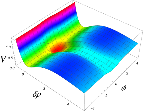
Figure 7: The potential of the volume modulus $\delta\rho$ and the inflaton $\phi$ in KKLT case, (68),(69). $V_{\rm inf}$ is chosen to be the form $V_{\rm inf}=V_{0}(1+\frac{\mu^{4}}{\phi^{4}})^{-1}$. Inflation is realized along the straight valley of the $\phi$ direction, while the volume $\delta\rho$ is stabilized. In realistic models one should take $V_{0}\sim 10^{{-10}}$; here we took $V_{0}=1$ just for illustration. The shape of the potential along the inflationary valley in the $\phi$ direction is shown by the dark blue line in Fig. 5.

Let us first consider the simplest case $f=0$ and $\chi=0$. In this case, the scalar potential is simply given by

$$V_{KKLT}=\frac{\mu^{4}}{(2\rho)^{3-\beta}}+\frac{aAe^{-a\rho}(-3W_{0}+Ae^{-a\rho}(3+a\rho))}{6\rho^{2}},$$ (70)

where we have minimized with respect to $\sigma$ and $\rho_{0}$ is the value at which $D_{T}W=0$ is satisfied. We denote the minimum of this potential as $\rho=\rho_{0}$, which satisfies

$$W_{0}=\frac{1}{3}Ae^{-a\rho_{0}}(3+2a\rho_{0})-\frac{2^{-2+\beta}e^{a\rho_{0}}(-3+\beta)\mu^{4}\rho_{0}^{\beta-1}}{aA(2+a\rho_{0})}.$$ (71)

We assume that $f(\chi)=0$ at the minimum of $\chi$. From (almost) vanishing cosmological constant condition, we find

$$\mu^{4}\simeq\frac{2^{2-\beta}a^{2}A^{2}e^{-2a\rho_{0}}\rho_{0}^{2-\beta}(2+a\rho_{0})}{3(-1+\beta+a\rho_{0})}.$$ (72)

For simplicity, let us choose $\beta=1$, and one finds

$$m_{3/2}=\frac{2Ae^{-a\rho_{0}}(1+a\rho_{0})}{6\sqrt{2}\rho_{0}^{3/2}}.$$ (73)

Tuning on the inflaton dependence $f$, the potential minimum of $\rho$ is no longer $\rho=\rho_{0}$. Let us call the deviation from $\rho_{0}$ as $\delta\rho$. We expand the potential with respect to $\delta\rho$ and minimize it, which gives the following effective potential,

$$V_{\rm eff}= \frac{24am_{3/2}^{2}\rho_{0}^{4}(2+a\rho_{0})f}{(1+a\rho_{0}))^{2}}-\frac{48m_{3/2}^{2}\rho_{0}^{2}(2+a\rho_{0})^{2}f^{2}}{a(1+a\rho_{0})^{2}(3+2a\rho_{0})}$$

$$= V_{\rm inf}-\frac{2V_{\rm inf}^{2}(1+a\rho_{0})^{2}}{3a^{3}\rho_{0}^{3}(3+2a\rho_{0})m_{3/2}^{2}}.$$ (74)

Here we have set $\chi=0$, which is justified below, and defined

$$V_{\rm inf}=\frac{24am_{3/2}^{2}\rho_{0}^{4}(2+a\rho_{0})f}{(1+a\rho_{0})^{2}}.$$

The second term is regarded as the deformation of potential from the back-reaction of heavy modulus $\rho$. We find that the back-reaction term has the factor $V_{\rm inf}/{m_{3/2}^{2}}\sim H^{2}_{\rm inf}/m_{3/2}^{2}$. We remind here that KKLT uplift is consistent with inflation only if the height of the barrier is higher than the scale of inflation, $m_{3/2}>H_{\rm inf}$ Kallosh:2004yh . Thus, in our case $H^{2}_{\rm inf}/m_{3/2}^{2}$ must be small (i.e. SUSY breaking must be higher than inflation scale), which also protects the system from back-reaction.

Finally, let us comment on the stability of sinflaton $\chi$. Near the minimum $\delta\rho\sim 0$, the mass of sinflaton is given by

$$m_{\chi}^{2}=K^{\Phi\bar{\Phi}}V_{\phi\phi}=\frac{4(3a^{2}\rho_{0}^{2}m_{3/2}^{2}+2V_{\rm inf}(1+a\rho_{0})^{2})}{3(1+a\rho_{0})^{2}}.$$ (75)

Thus, the sinflaton mass is always greater than inflation scale, and the sinflaton can be set at its origin.

6.4 KL model

Next, we consider inflation coupled to KL moduli stabilization Kallosh:2004yh . The system is given by

$$K= -3\log(T+\bar{T}-(\Phi+\bar{\Phi})^{2})+\frac{S\bar{S}}{(T+\bar{T}-(\Phi+\bar{\Phi})^{2})^{\beta}(1+f(\Phi,\bar{\Phi}))},$$ (76)

$$W= W_{0}-Ae^{-aT}+Be^{-bT}+\delta w+\mu^{2}S.$$ (77)

We focus on the vacuum where

$$Ae^{-aT}\sim Be^{-bT}\sim W_{0}\gg\delta w.$$

In particular, we assume the relation

$$W_{0}=A\left(\frac{aA}{bB}\right)^{-\frac{a}{a-b}}\left(1-\frac{a}{b}\right).$$

This relation leads to $W=0$ when $\delta w=0=W_{T}$ is satisfied. One can check that $\sigma=0$ is the minimum.

As previous case, we expand the potential in $\delta\rho=\rho-\rho_{0}$ up to the quadratic order, where $\rho_{0}$ is the value of $\rho$ for the case with $\chi=f=0$. By minimizing the potential with respect to $\delta\rho$, we find the following effective potential,

$$V_{\rm eff}=3m_{3/2}^{2}(1+\cdots)f-\frac{6(3-\beta)^{2}m_{3/2}^{4}f^{2}}{M^{2}\rho_{0}}+\cdots,$$ (78)

where $M=\frac{2}{3}aA(a-b)(\frac{aA}{bB})^{-\frac{a}{a-b}}$ is the mass of $\rho$ at $\delta w=\mu=0$. The ellipses denote the higher order terms suppressed by the factor $m_{3/2}/M$. For $M\gg m_{3/2}$, the leading part of the effective potential is $V_{\rm inf}=3m_{3/2}^{2}f$. We rewrite the effective potential as

$$V_{\rm eff}\sim V_{\rm inf}-\frac{2V_{\rm inf}^{2}}{3M^{2}}.$$ (79)

The moduli stabilization during inflation requires $H_{\rm inf}\ll M$, and this condition means that the second term in the effective potential is much smaller than the leading term. Thus, we can safely ignore the correction coming from the back-reaction of the heavy modulus $\rho$. Note that in KL model the mass $M$ is not related to the mass of gravitino. This allows much greater flexibility with respect to the strength of SUSY breaking.

Finally, we note that the mass of $\chi$ near $\delta\rho=0$ is given by

$$m_{\chi}^{2}=(8+12f)m^{2}_{3/2}=8m_{3/2}^{2}+4V_{\rm inf}.$$ (80)

Therefore, $\chi$ is stabilized at its origin during inflation with a sufficiently large mass. The shape of the potential in this model is very similar to the one shown in Fig. 7.

7 Discussion

During the last 15 years the accuracy of determination of the spectral parameter $n_{s}$ increased dramatically. In 2003, after the first WMAP data release, the combination of all available data suggested that $n_{s}=0.93\pm 0.03$ Spergel:2003cb . 9 years later, in the 9 year WMAP data release, the result was $n_{s}=0.972\pm 0.013$ Hinshaw:2012aka . In the Planck 2013 data release the corresponding number was $n_{s}=0.9603\pm 0.0073$ Ade:2013zuv . Finally, the Planck 2018 result is $n_{s}=0.965\pm 0.004$ Aghanim:2018eyx .

There are many models where by tuning two or three parameters one can get $n_{s}=0.965\pm 0.004$, but typically this tuning additionally depends on $r$. As a result, most inflationary models have $n_{s}$ and $r$ all over the place in the $n_{s}$ - $r$ plane.

One of the rare exceptions is the class of $\alpha$-attractors Kallosh:2013yoa , which match the Planck 2018 data without any fine-tuning. Predictions of these models are shown, in the simplest case, in Fig. 1 by two yellow lines for $N_{e}=50,60$. For more general $\alpha$-attractor models, the predictions for $n_{s}$ and $r$ are shown in Fig. 3. In the large $N_{e}$ limit, they are given by

$${}^{\alpha}n_{s}\approx 1-{2\over N_{e}}\ ,\qquad^{\alpha}r\approx{12\alpha\over N_{e}^{2}}\ .$$ (81)

These models for small values of $r$ tend to cover the left side of the $1\sigma$ area in the Planck 2018 data, see Figs. 1, 2, 3, 4.

In this paper we revisited D-brane inflation models in string theory in the context of volume stabilization Kachru:2003sx ; Dvali:2001fw ; Burgess:2001fx ; GarciaBellido:2001ky . At a phenomenological level, the inflationary models with

$${}^{4}V_{\rm inf}=V_{0}\Big{[}1+\Big{(}{m\over\phi}\Big{)}^{4}\Big{]}^{-1}\,,\qquad^{2}V_{\rm inf}=V_{0}\Big{[}1+\Big{(}{m\over\phi}\Big{)}^{2}\Big{]}^{-1}\,,\qquad^{1}V_{\rm inf}=V_{0}\Big{[}1+\Big{(}{m\over|\phi|}\Big{)}\Big{]}^{-1}$$ (82)

have many nice features similar to those of the $\alpha$-attractors. Namely, as shown in Burgess:2001fx ; GarciaBellido:2001ky and in Kachru:2003sx , in inverse quartic case and in inverse quadratic case they have universal predictions for $m\lesssim 1$ at large $N_{e}$ and small $r$:

$${}^{4}n_{s}\approx 1-{5\over 3N_{e}}\,,\qquad^{4}r\approx{4m^{{4\over 3}}\over(3N_{e})^{5\over 3}}\ ,$$ (83)

and

$${}^{2}n_{s}\approx 1-{3\over 2N_{e}}\ ,\qquad^{2}r\approx{12\alpha\over N_{e}^{2}}\ .$$ (84)

We have also added the case of an inverse linear potential

$${}^{1}n_{s}\approx 1-{4\over 3N_{e}}\ ,\qquad^{1}r\approx{8m^{2\over 3}\over\left(3N_{e}\right)^{{3\over 4}}}\ .$$ (85)

These models have specific values of $n_{s}$ which nicely agree with the data, for any choice of parameters. In fact, this property is the same as in $\alpha$-attractor models.

Since $2>{5\over 3}>{3\over 2}$, we see that the ${}^{4}V_{\rm inf}$ slice of the $n_{s}$ - $r$ plane is to the right of the one for the $\alpha$-attractor models, and the predictions for ${}^{2}V_{\rm inf}$ are even more to the right. Adding the linear case, and since $2>{5\over 3}>{3\over 2}>{4\over 3}$ we note that this model is even more to the right, compared to $\alpha$-attractors, for the same values of $N_{e}$.

A combination of $\alpha$-attractors and the D-brane inflation with the inverse quartic potentials for KKLTI and BI models completely covers the $1\sigma$ sweet spot of the Planck data, and a combination of these models with KKLTI and BI models with quartic potentials almost completely covers the broader $2\sigma$ area of the Planck 2018 data, see Fig. 4. The missing in Fig. 4 linear case is a bit to the right from the quadratic one.

In view of phenomenological importance of the D-brane inflation models, we revisited their stringy origin. Based on the original Polchinski’s computation of D-brane-D-brane (vanishing) potential as well as the studies of this in Kachru:2003sx , we find that D-brane-anti-D-brane potential leads to a specific dependence on the open string modulus of the geometry of the nilpotent multiplet $K_{S\bar{S}}(z^{i},\bar{z}^{i};\Phi,\bar{\Phi})=\mu^{4}{e^{K(z^{i},\bar{z}^{i};\Phi,\bar{\Phi})}\over V_{\overline{D}_{3}}+V_{D3/\overline{D3}}(\Phi,\bar{\Phi})}$. This is our generalization, to the case of the open string moduli, of the dictionary between string theory models with local sources in ten dimensions and the four-dimensional de Sitter supergravity studied for closed string theory moduli in Kallosh:2018nrk .

We combined this geometric information with the shift symmetric Kähler  potential $K=-3\log(T+\bar{T}-(\Phi+\bar{\Phi})^{2})$ of the kind known for $K3\times{T^{2}\over\mathbb{Z}_{2}}$ compactification. The resulting de Sitter type supergravity models, with either KKLT or KL volume stabilization, were studied in the regime of strong volume stabilization. The combined potential of the inflaton and the volume modulus is shown in Fig. 7. One can see a nearly flat inflationary $\chi$ direction, with the D-brane inflaton potential remaining practically unchanged by the presence of the strongly stabilized volume modulus.

To complete this construction, it would be important to study quantum corrections of the type discussed in fiber inflation in Cicoli:2008gp ; Kallosh:2017wku and in D3/D7 model in Haack:2008yb , reviewed here in Sec. 4.1. It will also be important to study quantum corrections in case that KKLT-type volume stabilization proceeds via a superpotential generated by Euclidean D3-branes Witten:1996bn ; Gorlich:2004qm ; Bergshoeff:2005yp , not by gaugino condensation. This is a very challenging task, but the phenomenological success of the simple D-brane inflation models considered in this paper suggests that these theories deserve a detailed investigation.

Acknowledgments: We are grateful to D. Baumann, S. Ferrara, S. Kachru, J. Maldacena, L. McAllister, E. Silverstein, S. Trivedi, F. Zwirner, and T. Wrase for stimulating discussions and collaboration on related work. This work is supported by SITP and by the US National Science Foundation grant PHY-1720397 and by the Simons foundation grant.

Appendix A Other phenomenological models

We show different phenomenological models having the potential (61). The relation between string theory and the following models are not clear. Nevertheless, these phenomenological models are consistent with the current cosmological data and interesting independently of string theory.

A.1 From flattening mechanism

First, let us consider the following simple (but non-supersymmetric) system with two scalars $(\chi,\phi)$ with potential

$$V=\frac{1}{2}m^{2-2p}\phi^{2p}\chi^{2}+\frac{1}{2}M^{2}(\chi-\chi_{0})^{2}\ ,$$ (86)

where $M,\ m$ and $\chi_{0}$ are constants. First, we integrate out the heavy moduli $\chi$, and find the following effective potential

$$V_{\rm eff}=\frac{1}{2}M^{2}\chi_{0}^{2}\left(1+\frac{\mu^{2p}}{\phi^{2p}}\right)^{-1}\ .$$ (87)

Here we have neglected higher derivative corrections since they are smaller compared to the corrections to potential Dong:2010in .

A.2 Supergravity model

Next we consider a supergravity model with

$$K= \frac{1}{2}(\Phi+\bar{\Phi})^{2}+S\bar{S}+\left(1+\frac{(\Phi\bar{\Phi})^{p}}{M^{2p}}\right)Y\bar{Y},$$

$$W= \mu^{2}S+W_{0}+\lambda m^{2-p}\Phi^{p}Y,$$ (88)

where $X$ is a nilpotent superfield and $Y$ is a constrained superfield satisfying $XY=0$. Both $X$ and $Y$ do not have dynamical scalars, and $F^{X}\neq 0$ for consistency. $\Phi=\chi+i\phi$ and $\chi$ is the inflaton. The scalar potential becomes

$$V= (\mu^{4}-3W_{0}^{2})+\lambda^{2}m^{4-2p}\frac{|\Phi|^{2p}}{1+\frac{|\Phi|^{{2p}}}{M^{2p}}}$$

$$= \Lambda^{4}+\lambda^{2}(M^{p}m^{2-p})^{2}\left(1+\frac{M^{2p}}{|\Phi|^{2p}}\right)^{-1},$$ (89)

where $\Lambda^{4}=\mu^{4}-3W_{0}^{2}$ is a cosmological constant which is fine-tuned to be $\mathcal{O}(10^{-120})$. We expand the potential with respect to $\chi$, and find

$$V=V_{\rm inf}+\left(4W_{0}^{2}+V_{\rm inf}\left(2+\frac{pM^{2p}}{\phi^{2}(M^{2p}+\phi^{2p})}\right)\right)\chi^{2}+\mathcal{O}(\chi^{4}),$$ (90)

where

$$V_{\rm inf}=\lambda^{2}(m^{2-p}M^{p})^{2}\left(1+\frac{M^{2p}}{\phi^{2p}}\right)^{-1}.$$ (91)

Thus, the sinflaton $\chi$ is stabilized at $\chi=0$ during inflation, and we find a single-field inflation with the KKLTI potential.

References

- (1) Planck collaboration, Y. Akrami et al., Planck 2018 results. X. Constraints on inflation, 1807.06211.
- (2) R. Kallosh, A. Linde and D. Roest, Superconformal Inflationary -Attractors, JHEP 11 (2013) 198, [1311.0472].
- (3) A. A. Starobinsky, A New Type of Isotropic Cosmological Models Without Singularity, Phys. Lett. 91B (1980) 99–102.
- (4) A. S. Goncharov and A. D. Linde, CHAOTIC INFLATION OF THE UNIVERSE IN SUPERGRAVITY, Sov. Phys. JETP 59 (1984) 930–933.
- (5) D. S. Salopek, J. R. Bond and J. M. Bardeen, Designing Density Fluctuation Spectra in Inflation, Phys. Rev. D40 (1989) 1753.
- (6) F. L. Bezrukov and M. Shaposhnikov, The Standard Model Higgs boson as the inflaton, Phys. Lett. B659 (2008) 703–706, [0710.3755].
- (7) J. J. M. Carrasco, R. Kallosh and A. Linde, -Attractors: Planck, LHC and Dark Energy, JHEP 10 (2015) 147, [1506.01708].
- (8) R. Kallosh and A. Linde, Universality Class in Conformal Inflation, JCAP 1307 (2013) 002, [1306.5220].
- (9) M. Cicoli, C. P. Burgess and F. Quevedo, Fibre Inflation: Observable Gravity Waves from IIB String Compactifications, JCAP 0903 (2009) 013, [0808.0691].
- (10) R. Kallosh, A. Linde, D. Roest, A. Westphal and Y. Yamada, Fibre Inflation and -attractors, JHEP 02 (2018) 117, [1707.05830].
- (11) S. Ferrara and R. Kallosh, Seven-Disk Manifold, -attractors and B-modes, 1610.04163.
- (12) R. Kallosh, A. Linde, T. Wrase and Y. Yamada, Maximal Supersymmetry and B-Mode Targets, JHEP 04 (2017) 144, [1704.04829].
- (13) S. Kachru, R. Kallosh, A. D. Linde, J. M. Maldacena, L. P. McAllister and S. P. Trivedi, Towards inflation in string theory, JCAP 0310 (2003) 013, [hep-th/0308055].
- (14) L. Lorenz, J. Martin and C. Ringeval, Brane inflation and the WMAP data: A Bayesian analysis, JCAP 0804 (2008) 001, [0709.3758].
- (15) J. Martin, C. Ringeval and V. Vennin, Encyclopædia Inflationaris, Phys. Dark Univ. 5-6 (2014) 75–235, [1303.3787].
- (16) G. R. Dvali, Q. Shafi and S. Solganik, D-brane inflation, in 4th European Meeting From the Planck Scale to the Electroweak Scale (Planck 2001) La Londe les Maures, Toulon, France, May 11-16, 2001, 2001, hep-th/0105203.
- (17) C. P. Burgess, M. Majumdar, D. Nolte, F. Quevedo, G. Rajesh and R.-J. Zhang, The Inflationary brane anti-brane universe, JHEP 07 (2001) 047, [hep-th/0105204].
- (18) J. Garcia-Bellido, R. Rabadan and F. Zamora, Inflationary scenarios from branes at angles, JHEP 01 (2002) 036, [hep-th/0112147].
- (19) D. Baumann, A. Dymarsky, I. R. Klebanov and L. McAllister, Towards an Explicit Model of D-brane Inflation, JCAP 0801 (2008) 024, [0706.0360].
- (20) D. Baumann and L. McAllister, Inflation and String Theory. Cambridge Monographs on Mathematical Physics. Cambridge University Press, 2015, 10.1017/CBO9781316105733.
- (21) E. Silverstein and A. Westphal, Monodromy in the CMB: Gravity Waves and String Inflation, Phys. Rev. D78 (2008) 106003, [0803.3085].
- (22) L. McAllister, E. Silverstein and A. Westphal, Gravity Waves and Linear Inflation from Axion Monodromy, Phys. Rev. D82 (2010) 046003, [0808.0706].
- (23) X. Dong, B. Horn, E. Silverstein and A. Westphal, Simple exercises to flatten your potential, Phys. Rev. D84 (2011) 026011, [1011.4521].
- (24) L. McAllister, E. Silverstein, A. Westphal and T. Wrase, The Powers of Monodromy, JHEP 09 (2014) 123, [1405.3652].
- (25) R. Kallosh and T. Wrase, dS Supergravity from 10d, Fortsch. Phys. 2018 (2018) 1800071, [1808.09427].
- (26) J. Blaback, U. Danielsson and G. Dibitetto, A new light on the darkest corner of the landscape, 1810.11365.
- (27) J. Polchinski, Tasi lectures on D-branes, in Fields, strings and duality. Proceedings, Summer School, Theoretical Advanced Study Institute in Elementary Particle Physics, TASI’96, Boulder, USA, June 2-28, 1996, pp. 293–356, 1996, hep-th/9611050.
- (28) C. P. Bachas, Lectures on D-branes, in Duality and supersymmetric theories. Proceedings, Easter School, Newton Institute, Euroconference, Cambridge, UK, April 7-18, 1997, pp. 414–473, 1998, hep-th/9806199.
- (29) E. Kiritsis, Introduction to superstring theory, vol. B9 of Leuven notes in mathematical and theoretical physics. Leuven U. Press, Leuven, 1998.
- (30) K. Dasgupta, C. Herdeiro, S. Hirano and R. Kallosh, D3 / D7 inflationary model and M theory, Phys. Rev. D65 (2002) 126002, [hep-th/0203019].
- (31) J. P. Hsu, R. Kallosh and S. Prokushkin, On brane inflation with volume stabilization, JCAP 0312 (2003) 009, [hep-th/0311077].
- (32) J. P. Hsu and R. Kallosh, Volume stabilization and the origin of the inflaton shift symmetry in string theory, JHEP 04 (2004) 042, [hep-th/0402047].
- (33) R. Kallosh, On inflation in string theory, Lect. Notes Phys. 738 (2008) 119–156, [hep-th/0702059].
- (34) M. Haack, R. Kallosh, A. Krause, A. D. Linde, D. Lust and M. Zagermann, Update of D3/D7-Brane Inflation on K3 x T**2/Z(2), Nucl. Phys. B806 (2009) 103–177, [0804.3961].
- (35) M. Berg, M. Haack and B. Kors, Loop corrections to volume moduli and inflation in string theory, Phys. Rev. D71 (2005) 026005, [hep-th/0404087].
- (36) L. McAllister, An Inflaton mass problem in string inflation from threshold corrections to volume stabilization, JCAP 0602 (2006) 010, [hep-th/0502001].
- (37) M. Berg, M. Haack and B. Kors, String loop corrections to Kahler potentials in orientifolds, JHEP 11 (2005) 030, [hep-th/0508043].
- (38) E. Witten, Nonperturbative superpotentials in string theory, Nucl. Phys. B474 (1996) 343–360, [hep-th/9604030].
- (39) L. Gorlich, S. Kachru, P. K. Tripathy and S. P. Trivedi, Gaugino condensation and nonperturbative superpotentials in flux compactifications, JHEP 12 (2004) 074, [hep-th/0407130].
- (40) E. Bergshoeff, R. Kallosh, A.-K. Kashani-Poor, D. Sorokin and A. Tomasiello, An Index for the Dirac operator on D3 branes with background fluxes, JHEP 10 (2005) 102, [hep-th/0507069].
- (41) S. Ferrara, R. Kallosh and A. Linde, Cosmology with Nilpotent Superfields, JHEP 10 (2014) 143, [1408.4096].
- (42) R. Kallosh and T. Wrase, Emergence of Spontaneously Broken Supersymmetry on an Anti-D3-Brane in KKLT dS Vacua, JHEP 12 (2014) 117, [1411.1121].
- (43) E. A. Bergshoeff, K. Dasgupta, R. Kallosh, A. Van Proeyen and T. Wrase, and dS, JHEP 05 (2015) 058, [1502.07627].
- (44) R. Kallosh, F. Quevedo and A. M. Uranga, String Theory Realizations of the Nilpotent Goldstino, JHEP 12 (2015) 039, [1507.07556].
- (45) E. A. Bergshoeff, D. Z. Freedman, R. Kallosh and A. Van Proeyen, Pure de Sitter Supergravity, Phys. Rev. D92 (2015) 085040, [1507.08264].
- (46) F. Hasegawa and Y. Yamada, Component action of nilpotent multiplet coupled to matter in 4 dimensional supergravity, JHEP 10 (2015) 106, [1507.08619].
- (47) D. V. Volkov and V. P. Akulov, Possible universal neutrino interaction, JETP Lett. 16 (1972) 438–440.
- (48) E. McDonough and M. Scalisi, Inflation from Nilpotent Kähler Corrections, JCAP 1611 (2016) 028, [1609.00364].
- (49) R. Kallosh, A. Linde, D. Roest and Y. Yamada, induced geometric inflation, JHEP 07 (2017) 057, [1705.09247].
- (50) S. Kachru, R. Kallosh, A. D. Linde and S. P. Trivedi, De Sitter vacua in string theory, Phys. Rev. D68 (2003) 046005, [hep-th/0301240].
- (51) R. Kallosh, A. Linde, K. A. Olive and T. Rube, Chaotic inflation and supersymmetry breaking, Phys. Rev. D84 (2011) 083519, [1106.6025].
- (52) A. Linde, Y. Mambrini and K. A. Olive, Supersymmetry Breaking due to Moduli Stabilization in String Theory, Phys. Rev. D85 (2012) 066005, [1111.1465].
- (53) E. Dudas, A. Linde, Y. Mambrini, A. Mustafayev and K. A. Olive, Strong moduli stabilization and phenomenology, Eur. Phys. J. C73 (2013) 2268, [1209.0499].
- (54) R. Kallosh and A. D. Linde, Landscape, the scale of SUSY breaking, and inflation, JHEP 12 (2004) 004, [hep-th/0411011].
- (55) J. J. Blanco-Pillado, R. Kallosh and A. D. Linde, Supersymmetry and stability of flux vacua, JHEP 05 (2006) 053, [hep-th/0511042].
- (56) R. Kallosh, A. Linde, B. Vercnocke and T. Wrase, Analytic Classes of Metastable de Sitter Vacua, JHEP 10 (2014) 011, [1406.4866].
- (57) F. Hasegawa, K. Nakayama, T. Terada and Y. Yamada, Gravitino problem in inflation driven by inflaton-polonyi Kähler coupling, Phys. Lett. B777 (2018) 270–274, [1709.01246].
- (58) WMAP collaboration, D. N. Spergel et al., First year Wilkinson Microwave Anisotropy Probe (WMAP) observations: Determination of cosmological parameters, Astrophys. J. Suppl. 148 (2003) 175–194, [astro-ph/0302209].
- (59) WMAP collaboration, G. Hinshaw et al., Nine-Year Wilkinson Microwave Anisotropy Probe (WMAP) Observations: Cosmological Parameter Results, Astrophys. J. Suppl. 208 (2013) 19, [1212.5226].
- (60) Planck collaboration, P. A. R. Ade et al., Planck 2013 results. XVI. Cosmological parameters, Astron. Astrophys. 571 (2014) A16, [1303.5076].
- (61) Planck collaboration, N. Aghanim et al., Planck 2018 results. VI. Cosmological parameters, 1807.06209.