Simple Attention-Based Representation Learning for
Ranking Short Social Media Posts

Abstract

This paper explores the problem of ranking short social media posts with respect to user queries using neural networks. Instead of starting with a complex architecture, we proceed from the bottom up and examine the effectiveness of a simple, word-level Siamese architecture augmented with attention-based mechanisms for capturing semantic “soft” matches between query and post tokens. Extensive experiments on datasets from the TREC Microblog Tracks show that our simple models not only achieve better effectiveness than existing approaches that are far more complex or exploit a more diverse set of relevance signals, but are also much faster. Implementations of our samCNN (Simple Attention-based Matching CNN) models are shared with the community to support future work.

1 Introduction

Despite a large body of work on neural ranking models for “traditional” ad hoc retrieval over web pages and newswire documents (Huang et al., 2013; Shen et al., 2014; Guo et al., 2016; Xiong et al., 2017; Mitra et al., 2017; Pang et al., 2017; Dai et al., 2018; McDonald et al., 2018), there has been surprisingly little work Rao et al. (2017) on applying neural networks to searching short social media posts such as tweets on Twitter. Rao et al. (2019) identified short document length, informality of language, and heterogeneous relevance signals as main challenges in relevance modeling, and proposed the first neural model specifically designed to handle these characteristics. Evaluation on a number of datasets from the TREC Microblog Tracks demonstrates state-of-the-art effectiveness as well as the necessity of different model components to capture a multitude of relevance signals.

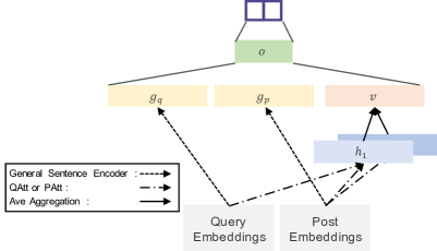
Figure 1: Our model architecture: a general sentence encoder is applied on query and post embeddings to generate $\textbf{g}_{q}$ and $\textbf{g}_{p}$; an attention encoder is applied on post embeddings to generate variable-length query-aware features ${\textbf{h}_{i}}$. These features are further aggregated to yield v, which feeds into the final prediction.

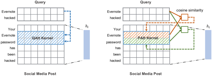
Figure 2: The Query-Aware Attention (QAtt) architecture on the left and the Position-Aware Attention (PAtt) architecture on the right. In both, we construct $F$ convolutional kernels for each query token (here, one kernel for the query token ‘Evernote’ is visualized). In QAtt, the query token embedding is directly “injected” into the kernel via element-wise product (blue dotted arrows). In PAtt, cosine similarity between the query token and tokens in the post within the convolution window are used as attention weights in the kernel.

In this paper, we also examine the problem of modeling relevance for ranking short social media posts, but from a complementary perspective. As Weissenborn et al. (2017) notes, most systems are built in a top-down process: authors propose a complex architecture and then validate design decisions with ablation experiments. However, such experiments often lack comparisons to strong baselines, which raises the question as to whether model complexity is empirically justified. As an alternative, they advocate a bottom-up approach where architectural complexity is gradually increased. We adopt exactly such an approach, focused exclusively on word-level modeling. As shown in Figure 1, we examine variants of a simple, generic architecture that has emerged as “best practices” in the NLP community for tackling modeling problems on two input sequences: a Siamese CNN architecture for learning representations over both inputs (a query and a social media post in our case), followed by fully-connected layers that produce a final relevance prediction (Severyn and Moschitti, 2015; He et al., 2016; Rao et al., 2016), which we refer to as a General Sentence Encoder in Section 2.1. Further adopting best practices, we incorporate query-aware convolutions with an average aggregation layer in the representation learning process.

Recently, a number of researchers (Conneau et al., 2017; Mohammed et al., 2018) have started to reexamine simple baselines and found them to be highly competitive with the state of the art, especially with proper tuning. For example, the InferSent approach Conneau et al. (2017) uses a simple BiLSTM with max pooling that achieves quite impressive accuracy on several classification benchmarks. Our contribution is along similar lines, where we explore simple yet highly effective models for ranking social media posts, to gain insights into query–post relevance matching using standard neural architectures. Experiments with TREC Microblog datasets show that our best model not only achieves better effectiveness than existing approaches that leverage more signals, but also demonstrates 4$\times$ speedup in model training and inference compared to a recently-proposed neural model.

2 Model

Our model comprises a representation learning layer with convolutional encoders and another simple aggregation layer. These architectural components are described in detail below.

2.1 Representation Learning Layer

General Sentence Encoder: The general sentence encoder uses a standard convolutional layer with randomly initialized kernels to learn semantic representations for text. More formally, given query $q$ and post $p$ as sentence inputs, we first convert them to embedding matrices Q and P through an embedding lookup layer, where $\textbf{Q}\in\mathbb{R}^{n\times d}$ and $\textbf{P}\in\mathbb{R}^{m\times d}$, $d$ is the dimension of embeddings, and $n$ and $m$ are the number of tokens in $q$ and $p$, respectively. Then we apply a standard convolution operation with kernel window size $k$ over the embedding matrix Q and P. The convolution operation is parameterized by a weight term $\textbf{W}\in\mathbb{R}^{F\times k\times d}$ and a bias term $\textbf{$b_{w}$}\in\mathbb{R}^{F}$, where $F$ is the number of convolutional kernels. This generates semantic representation $\textbf{O}_{q}\in\mathbb{R}^{n\times F}$ and $\textbf{O}_{p}\in\mathbb{R}^{m\times F}$, on which max pooling and an MLP are applied to obtain query representation $\textbf{g}_{q}\in\mathbb{R}^{d}$ and post representation $\textbf{g}_{p}\in\mathbb{R}^{d}$.

The weakness of the kernels in the general sentence encoder is that they do not incorporate knowledge from the query when attempting to capture feature patterns from the post. Inspired by attention mechanisms Bahdanau et al. (2014), we propose two novel approaches to incorporate query information when encoding the post representation, which we introduce below.

Query-Aware Attention Encoder (QAtt): In QAtt (Figure 2, left), for each query token, we construct a token-specific convolutional kernel to “inject” the query information. Unlike methods that apply attention mechanisms after the sentence representations are generated Bahdanau et al. (2014); Seo et al. (2016), our approach aims to model the representation learning process jointly with an attention mechanism.

Formally, for each query token $t_{q}$, the QAtt kernel $\mathbf{W}_{\textrm{QAtt}}^{t_{q}}$ is composed as follows:

$$\mathbf{W}_{\textrm{QAtt}}^{t_{q}}=\mathbf{U}\otimes\mathbf{Q}_{t_{q}}$$ (1)

where $\mathbf{U}\in\mathbb{R}^{F\times k\times d}$ represents trainable parameters, $\mathbf{Q}_{t_{q}}$ is the embedding of token $t_{q}$ with size $\mathbb{R}^{d}$ and $\mathbf{W}_{\textrm{QAtt}}^{t_{q}}\in\mathbb{R}^{F\times k\times d}$. The element-wise product $\otimes$ is applied between the token embedding $\mathbf{Q}_{t_{q}}$ and the last dimension of kernel weights $\mathbf{U}$. In other words, we create $F$ convolutional kernels for each query token, where each kernel is “injected” with the embedding of that query token via element-wise product. Figure 2 (left) illustrates one kernel for the query token ‘Evernote’, where element-wise product is represented by blue dotted arrows. When a QAtt token-specific kernel is applied, a window slides across the post embeddings P and learns soft matches to each query token to generate query-aware representations.

On top of the QAtt kernels, we apply max-pooling and an MLP to produce a set of post representations $\{\textbf{h}_{i}\}$, with each $\textbf{h}_{i}\in\mathbb{R}^{d}$ standing for the representation learned from query token $t_{q_{i}}$.

Position-Aware Attention Encoder (PAtt): In the QAtt encoder, token-specific kernels learn soft matches to the query. However, they still ignore positional information when encoding the post semantics, which has been shown to be effective for sequence modeling Gehring et al. (2017). To overcome this limitation, we propose an alternative attention encoder that captures positional information through interactions between query embeddings and post embeddings.

Given a query token $t_{q}$ and the $j$-th position in post $p$, we compute the interaction scores by taking the cosine similarity between the word embeddings of token $t_{q}$ and post tokens $t_{p_{j:j+k-1}}$ from position $j$ to $j+k-1$:

$$S_{j}=[\textrm{cos}(t_{q},t_{p_{j}});...;\textrm{cos}(t_{q},t_{p_{j+k-1}})]$$ (2)

where $S_{j}\in\mathbb{R}^{k\times 1}$ and $k$ is the width of the convolutional kernel we are learning. That is, for each token in the post within the window, we compute its cosine similarity with query token $t_{q}$. We then convert the similarity vector $S_{j}$ into a matrix:

$$\hat{S}_{j}=S_{j}\cdot\mathds{1},\hat{S}_{j}\in\mathbb{R}^{k\times d}$$ (3)

where $\mathds{1}\in\mathbb{R}^{1\times d}$ with each element set to 1. Finally, the PAtt convolutional kernel for query token $t_{q}$ at the $j$-th position is constructed as:

$$\mathbf{W}_{\textrm{PAtt}}^{t_{q},j}=\mathbf{V}\otimes\hat{S}_{j}$$ (4)

where $\mathbf{V}\in\mathbb{R}^{F\times k\times d}$ represents the trainable parameters. The element-wise product $\otimes$ is applied between the attention weights $\hat{S}_{j}$ and the last two dimensions of kernel weights $\mathbf{V}$.

Conceptually, this operation can be thought as adding a soft attention weight (with values in the range of $[0,1]$) to each convolutional kernel, where the weight is determined by the cosine similarity between the token from the post and a particular query token; since cosine similarity is a scalar, we fill in the value in all $d$ dimensions of the kernel, where $d$ is the size of the word embedding. This is illustrated in Figure 2 (right), where we show one kernel of width two for the query token ‘Evernote’. The brown (green) arrows capture cosine similarity between the query token ‘Evernote’ and the first (second) token from the post in the window. These values then serve as weights in the kernels, shown as the hatched areas. Similar to QAtt, the PAtt encoder with max-pooling and an MLP generates a set of post representations $\{\textbf{h}_{i}\}$, with each $\textbf{h}_{i}$ standing for the representation learned from query token $t_{q_{i}}$.

It is worth noting that both the QAtt and PAtt encoders have no extra parameters over a general sentence encoder. However, incorporating the query-aware and position-aware information enables more effective representation learning, as our experiments show later. The QAtt and PAtt encoders can also be used as plug-in modules in any standard convolutional architecture to learn query-biased representations.

2.2 Aggregation Layer

After the representation layer, a set of vectors $\{\textbf{g}_{q},\textbf{g}_{p},\{\textbf{h}_{i}\}\}$ is obtained. Because our model yields different numbers of $\textbf{h}_{i}$ with queries of different lengths, further aggregation is needed to output a global feature v. We directly average all vectors $\mathbf{v}=\frac{1}{N_{q}}\sum{\mathbf{h_{i}}}$ as the aggregated feature, where $N_{q}$ is the length of the query.

2.3 Training

To obtain a final relevance score, the feature vectors $\textbf{g}_{q}$, $\textbf{g}_{p}$, and v are concatenated and fed into an MLP with ReLU activation for dimensionality reduction to obtain o, followed by batch normalization and fully-connected layer and softmax to output the final prediction. The model is trained end-to-end with a Stochastic Gradient Decent optimizer using negative log-likelihood loss.

Year	2011	2012	2013	2014
# queries	49	60	60	55
# tweets	39,780	49,879	46,192	41,579
# relevant	1,940	4,298	3,405	6,812
%relevant	4.87	8.62	7.37	16.38

Table 1: Statistics of TREC MB 2011–2014 datasets.

Param	Value	Param	Value
Embedding size	300	$k$	0.05
Hidden size	200	Final hidden size	100
Kernel number	250	Dropout ratio	0.5
Kernel size	2	Learning rate	0.03

Table 2: Hyperparameters for our models. GloVe (Pennington et al., 2014) embeddings are used and fine-tuned during training. Unknown words are initialized from a uniform distribution $[-k,k]$.

3 Experimental Setup

		2011		2012		2013		2014
		P30	AP	P30	AP	P30	AP	P30	AP
Our Models
1	BiCNN	0.2129	0.1634	0.2028	0.1176	0.2367	0.1284	0.3788	0.2557
2	BiCNN+QAtt	$0.3966^{1}$	$0.3586^{1}$	$0.3904^{1}$	$0.2376^{1}$	$0.4861^{1}$	$0.2696^{1}$	$0.6388^{1}$	$0.4226^{1}$
3	BiCNN+PAtt	$0.4469^{1,2}$	$0.4135^{1,2}_{5}$	$0.4017^{1}_{5}$	$0.2413^{1,5}$	$0.5167^{1,2}_{5}$	$0.2817^{1,2}$	$0.6642^{1,2}$	$0.4351^{1,2}_{5}$
4	BiCNN+PAtt+QL	$\textbf{0.4735}^{1{\text{-}}3}_{5{\text{-}}7}$	$\textbf{0.4346}^{1{\text{-}}3}_{5,6}$	$\textbf{0.4164}^{1,2}_{5,6}$	$\textbf{0.2516}^{1{\text{-}}3}_{5}$	$0.5256^{1{\text{-}}3}_{5,6}$	$\textbf{0.2965}^{1{\text{-}}3}_{5}$	$\textbf{0.6752}^{1,2}$	$\textbf{0.4522}^{1{\text{-}}3}_{5,7}$
Existing Models
5	QL	$0.4000^{1}$	$0.3576^{1}$	$0.3311^{1}$	$0.2091^{1}$	$0.4450^{1}$	$0.2532^{1}$	$0.6182^{1}$	$0.3924^{1}$
6	RM3	$0.4211^{1}$	$0.3824^{1}$	$0.3452^{1}$	$0.2342^{1}$	$0.4733^{1}$	$0.2766^{1}$	$0.6339^{1}$	$0.4480^{1}$
7	MP-HCNN(+URL)	$0.4075^{1,2}$	$0.3832^{1,2}$	$0.3689^{1,5}$	$0.2337^{1,5}$	$0.5222^{1,2}_{5}$	$0.2818^{1,2}_{5}$	$0.6297^{1}$	$0.4304^{1}$
8	MP-HCNN(+URL)+QL	$0.4293^{1,2}_{5}$	$0.4043^{1,2}_{5,6}$	$0.3791^{1,5}_{6}$	$0.2460^{1,5}$	$\textbf{0.5294}^{1{\text{-}}3}_{5,6}$	$0.2896^{1,2}_{5}$	$0.6394^{1}$	$0.4420^{1,5}$

Table 3: Results of various models on the TREC Microblog Tracks datasets. Models 5–8 are copied from Rao et al. (2019); note that MP-HCNN exploits URL information (+URL). Models with +QL include interpolation with the QL baseline. BiCNN denotes our general sentence encoder architecture, with either query-aware attention (QAtt) or position-aware attention (PAtt). Superscripts and subscripts indicate the row indexes for which a metric difference is statistically significant at $p<0.05$.

Datasets and Hyperparameters. Our models are evaluated on four tweet test collections from the TREC 2011–2014 Microblog (MB) Tracks (Ounis et al., 2011; Soboroff et al., 2012; Lin and Efron, 2013; Lin et al., 2014). Each dataset contains around 50–60 queries; detailed statistics are shown in Table 1. As with Rao et al. (2019), we evaluated our models in a reranking task, where the inputs are up to the top 1000 tweets retrieved from “bag of words” ranking using query likelihood (QL). We ran four-fold cross-validation split by year (i.e., train on three years’ data, test on one year’s data) and followed Rao et al. (2019) for sampling validation sets. For metrics, we used average precision (AP) and precision at rank 30 (P30). We conducted Fisher’s two-sided, paired randomization tests (Smucker et al., 2007) to assess statistical significance at $p<0.05$. The best model hyperparameters are shown in Table 2.

Baselines. On top of QL, RM3 (Abdul-Jaleel et al., 2004) provides strong non-neural results using pseudo-relevance feedback. We also compared against MP-HCNN (Rao et al., 2019), the first neural model that captures specific characteristics of social media posts, which improves over many previous neural models, e.g., K-NRM (Xiong et al., 2017) and DUET (Mitra et al., 2017), by a significant margin. To the best of our knowledge, Rao et al. (2019) is the most effective neural model to date. We compared against two variants of MP-HCNN; MP-HCNN+QL includes a linear interpolation with QL scores.

4 Results and Discussion

Table 3 shows the effectiveness of all variants of our model, compared against previous results copied from Rao et al. (2019). Model 1 illustrates the effectiveness of the basic BiCNN model with a kernel window size of two; combining different window sizes Kim (2014) doesn’t yield any improvements. It appears that this model performs worse than the QL baseline.

Comparing Model 2 to Model 1, we find that query-aware kernels contribute significant improvements, achieving effectiveness comparable to the QL baseline. With Model 3, which captures positional information with the position-aware encoder, we obtain competitive effectiveness compared to Model 8, the full MP-HCNN model that includes interpolation with QL. Note that Model 8 leverages additional signals, including URL information, character-level encodings, and external term features such as tf–idf. With Model 4, which interpolates the position-aware encoder with QL, we obtain state-of-the-art effectiveness.

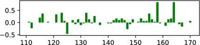
Figure 3: Per-query AP differences between PAtt and QL on TREC 2013 (queries 111–170).

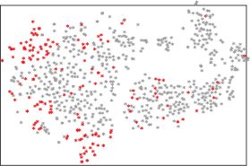
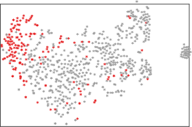
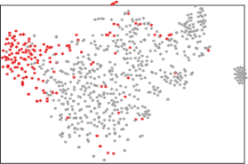
Figure 4: t-SNE visualizations of hidden states for the best-performing query 164 “lindsey vonn sidelined” from the basic BiCNN (left), QAtt (middle), and PAtt (right). Red (grey) dots represent relevant (non-relevant) posts.

Per-Query Analysis. In Figure 3, we show per-query AP differences between the PAtt model and the QL baseline on the TREC 2013 dataset. As we can see, PAtt improves on most of the queries. For the best-performing query 164 “lindsey vonn sidelined”, we project the hidden states o into a low-dimensional space using t-SNE Maaten and Hinton (2008), shown in Figure 4. We observe that with the basic BiCNN model (left), relevant posts are scattered. With the addition of an attention mechanism (either QAtt in the middle or PAtt on the right), most of the relevant posts are clustered together and separated from the non-relevant posts. With PAtt, there appears to be tighter clustering and better separation of the relevant posts from the non-relevant posts, giving rise to a better ranking. We confirmed similar behavior in many queries, which illustrates the ability of our position-aware attention encoder to learn better query-biased representations compared to the other two models.

Match	Count
Oscars	28
snub	20
Affleck	25
Oscars snub	18
snub Affleck	15
Oscars Affleck	23
Oscars snub Affleck	13

Table 4: Matching patterns for the worst-performing query 127 “Oscars snub Affleck”.

For the worst-performing query 125 “Oscars snub Affleck”, the PAtt model lost 0.47 in AP and 0.11 in P30. To diagnose what went wrong, we sampled the top 30 posts ranked by the PAtt model and counted the number of posts that contain different combinations of the query terms in Table 4. The PAtt model indeed captures matching patterns, mostly on Oscars and Affleck. However, from the relevance judgments we see that snub is the dominant term in most relevant posts, while Oscars is often expressed implicitly. For example, QL assigns more weight to the term snub in the relevant post “argo wins retributions for the snub of ben affleck” because of the term’s rarity; in contrast, the position-aware encoder places emphasis on the wrong query terms.

Model Performance. Finally, in terms of training and inference speed, we compared the PAtt model with MP-HCNN on a machine with a GeForce GTX 1080 GPU (batch size: 300). In addition to being more effective (as the above results show), PAtt is also approximately 4$\times$ faster.

5 Conclusions

In this paper, we proposed two novel attention-based convolutional encoders to incorporate query-aware and position-aware information with minimal additional model complexity. Results show that our model is simpler, faster, and more effective than previous neural models for searching social media posts.

References

- Abdul-Jaleel et al. (2004) Nasreen Abdul-Jaleel, James Allan, W. Bruce Croft, Fernando Diaz, Leah Larkey, Xiaoyan Li, Donald Metzler, Mark D. Smucker, Trevor Strohman, Howard Turtle, and Courtney Wade. 2004. UMass at TREC 2004: Novelty and HARD. In TREC.
- Bahdanau et al. (2014) Dzmitry Bahdanau, Kyunghyun Cho, and Yoshua Bengio. 2014. Neural machine translation by jointly learning to align and translate. arXiv:1409.0473.
- Conneau et al. (2017) Alexis Conneau, Douwe Kiela, Holger Schwenk, Loïc Barrault, and Antoine Bordes. 2017. Supervised learning of universal sentence representations from natural language inference data. In EMNLP, pages 670–680.
- Dai et al. (2018) Zhuyun Dai, Chenyan Xiong, Jamie Callan, and Zhiyuan Liu. 2018. Convolutional neural networks for soft-matching n-grams in ad-hoc search. In WSDM, pages 126–134.
- Gehring et al. (2017) Jonas Gehring, Michael Auli, David Grangier, Denis Yarats, and Yann N. Dauphin. 2017. Convolutional sequence to sequence learning. arXiv:1705.03122.
- Guo et al. (2016) Jiafeng Guo, Yixing Fan, Qingyao Ai, and W. Bruce Croft. 2016. A deep relevance matching model for ad-hoc retrieval. In CIKM, pages 55–64.
- He et al. (2016) Hua He, John Wieting, Kevin Gimpel, Jinfeng Rao, and Jimmy Lin. 2016. UMD-TTIC-UW at SemEval-2016 task 1: Attention-based multi-perspective convolutional neural networks for textual similarity measurement. In SemEval-2016, pages 1103–1108.
- Huang et al. (2013) Po-Sen Huang, Xiaodong He, Jianfeng Gao, Li Deng, Alex Acero, and Larry Heck. 2013. Learning deep structured semantic models for web search using clickthrough data. In CIKM, pages 2333–2338.
- Kim (2014) Yoon Kim. 2014. Convolutional neural networks for sentence classification. In EMNLP, pages 1746–1751.
- Lin and Efron (2013) Jimmy Lin and Miles Efron. 2013. Overview of the TREC-2013 Microblog Track. In TREC.
- Lin et al. (2014) Jimmy Lin, Miles Efron, Yulu Wang, and Garrick Sherman. 2014. Overview of the TREC-2014 Microblog Track. In TREC.
- Maaten and Hinton (2008) Laurens van der Maaten and Geoffrey Hinton. 2008. Visualizing data using t-SNE. Journal of machine learning research, 9:2579–2605.
- McDonald et al. (2018) Ryan McDonald, George Brokos, and Ion Androutsopoulos. 2018. Deep relevance ranking using enhanced document-query interactions. In EMNLP, pages 1849–1860.
- Mitra et al. (2017) Bhaskar Mitra, Fernando Diaz, and Nick Craswell. 2017. Learning to match using local and distributed representations of text for web search. In WWW, pages 1291–1299.
- Mohammed et al. (2018) Salman Mohammed, Peng Shi, and Jimmy Lin. 2018. Strong baselines for simple question answering over knowledge graphs with and without neural networks. In NAACL, pages 291–296.
- Ounis et al. (2011) Iadh Ounis, Craig Macdonald, Jimmy Lin, and Ian Soboroff. 2011. Overview of the TREC-2011 Microblog Track. In TREC.
- Pang et al. (2017) Liang Pang, Yanyan Lan, Jiafeng Guo, Jun Xu, Jingfang Xu, and Xueqi Cheng. 2017. DeepRank: A new deep architecture for relevance ranking in information retrieval. In CIKM, pages 257–266.
- Pennington et al. (2014) Jeffrey Pennington, Richard Socher, and Christopher Manning. 2014. GloVe: Global vectors for word representation. In EMNLP, pages 1532–1543.
- Rao et al. (2016) Jinfeng Rao, Hua He, and Jimmy Lin. 2016. Noise-contrastive estimation for answer selection with deep neural networks. In CIKM, pages 1913–1916.
- Rao et al. (2017) Jinfeng Rao, Hua He, Haotian Zhang, Ferhan Ture, Royal Sequiera, Salman Mohammed, and Jimmy Lin. 2017. Integrating lexical and temporal signals in neural ranking models for searching social media streams. arXiv:1707.07792.
- Rao et al. (2019) Jinfeng Rao, Wei Yang, Yuhao Zhang, Ferhan Ture, and Jimmy Lin. 2019. Multi-perspective relevance matching with hierarchical ConvNets for social media search. In AAAI.
- Seo et al. (2016) Minjoon Seo, Aniruddha Kembhavi, Ali Farhadi, and Hannaneh Hajishirzi. 2016. Bidirectional attention flow for machine comprehension. arXiv:1611.01603.
- Severyn and Moschitti (2015) Aliaksei Severyn and Alessandro Moschitti. 2015. Learning to rank short text pairs with convolutional deep neural networks. In SIGIR, pages 373–382.
- Shen et al. (2014) Yelong Shen, Xiaodong He, Jianfeng Gao, Li Deng, and Grégoire Mesnil. 2014. Learning semantic representations using convolutional neural networks for web search. In WWW, pages 373–374.
- Smucker et al. (2007) Mark D. Smucker, James Allan, and Ben Carterette. 2007. A comparison of statistical significance tests for information retrieval evaluation. In CIKM, pages 623–632.
- Soboroff et al. (2012) Ian Soboroff, Iadh Ounis, Craig Macdonald, and Jimmy Lin. 2012. Overview of the TREC-2012 Microblog Track. In TREC.
- Weissenborn et al. (2017) Dirk Weissenborn, Georg Wiese, and Laura Seiffe. 2017. Making neural QA as simple as possible but not simpler. In CoNLL, pages 271–280.
- Xiong et al. (2017) Chenyan Xiong, Zhuyun Dai, Jamie Callan, Zhiyuan Liu, and Russell Power. 2017. End-to-end neural ad-hoc ranking with kernel pooling. In SIGIR, pages 55–64.