Neural Likelihoods via Cumulative Distribution Functions

Abstract

We leverage neural networks as universal approximators of monotonic functions to build a parameterization of conditional cumulative distribution functions (CDFs). By the application of automatic differentiation with respect to response variables and then to parameters of this CDF representation, we are able to build black box CDF and density estimators. A suite of families is introduced as alternative constructions for the multivariate case. At one extreme, the simplest construction is a competitive density estimator against state-of-the-art deep learning methods, although it does not provide an easily computable representation of multivariate CDFs. At the other extreme, we have a flexible construction from which multivariate CDF evaluations and marginalizations can be obtained by a simple forward pass in a deep neural net, but where the computation of the likelihood scales exponentially with dimensionality. Alternatives in between the extremes are discussed. We evaluate the different representations empirically on a variety of tasks involving tail area probabilities, tail dependence and (partial) density estimation.

1 CONTRIBUTION

We introduce a novel parameterization of multivariate cumulative distribution functions (CDFs) using deep neural networks. We explain how training can be done by a straightforward adaptation of standard methods for neural networks. The main motivations behind our work include: a direct evaluation of tail area probabilities; coherent estimation of low dimensional marginals of a joint distribution without the requirement of fitting a full joint; and supervised/unsupervised density estimation.

The first two tasks benefit directly from a CDF computed by a forward pass in a neural network, as tail probabilities and marginal CDFs can be read-off essentially directly in this representation. The latter has been tackled by an increasingly large literature on neural density estimators. This dates back at least to Bishop (1994), who used multilayer perceptrons to encode conditional means, variances, and mixture probabilities for a (conditional) mixture of Gaussians. Recently, models using transformations of a simple distribution into more complex ones were proposed. Dinh et al. (2015),Dinh et al. (2017),Papamakarios et al. (2017), Huang et al. (2018) and De Cao and Titov (2019) are examples of the state of the art for density estimation. They use invertible transformations from simple base distributions where the determinant of the Jacobian is easy to compute and Monte Carlo approaches for computing gradients become feasible. Depending on the architecture, they are optimized for density estimation or sampling. We show we remain competitive against these methods while keeping a comparatively simple uniform structure with few hyperparameters. For instance, compared to the method of Bishop (1994), there is no need to choose the base distribution of the mixture nor the number of mixtures.

All of the above is predicated on how we construct multivariate CDFs. The most direct extension from univariate to multivariate CDFs is conceptually simple, but the calculation of the likelihood grows exponentially in the dimensionality. This is essentially the counterpart to computing a partition function in an undirected graphical model, where here the problem is differentiation as opposed to integration. Compromises are discussed, including the relationship to Gaussian copula models and other CDF constructions based on small dimensional marginals. One extreme sacrifices the ability of representing a CDF by a single forward pass in exchange for scalability to high dimensions, where we can compare it against state-of-the-art neural density estimators.

This paper is organized as follows. Section 2 describes our main approach. Related work is described in Sections 3 and S1. Experiments are discussed in Section 4. We show that our models are competitive for density estimation while able to directly tackle some modelling problems where recent neural-based models could not be applied in an obvious manner.

2 THE MONOTONIC NEURAL DENSITY ESTIMATOR

We now introduce the Monotonic Neural Density Estimator (MONDE), inspired by neural network methods for parameterizing monotonic functions. The primary usage of MONDE is to compute conditional CDFs with a single forward pass in a deep neural network, while allowing for the calculation of the corresponding conditional densities by tapping into existing methods for computing derivatives in deep learning. The latter is particularly relevant for likelihood-based fitting methods such as maximum (composite) likelihood. We will focus on the continuous case only, where probability density functions (pdfs) are defined, although extensions to include mixed combinations of discrete and continuous variables are straightforward by considering difference operations as opposed to differentiation operations. We start with the simplest but important univariate case, where dependency between variables does not have to be modelled. We progress through more complex constructions to conclude with the most flexible but computationally demanding case, where we deal with multivariate data without assuming any specific families of distributions for the data generating process.

Here we use the following notation.
$F(\mathbf{y}|\mathbf{x})$: multivariate conditional CDF, where $\mathbf{y}\in\mathbb{R}^{K}$ is the response vector and $\mathbf{x}\in\mathbb{R}^{D}$ is a covariate vector;
$F_{k}(y_{k}|\mathbf{x})$: $k$-th marginal conditional CDF;
$f(\mathbf{y}|\mathbf{x})$: multivariate conditional pdf;
$f_{k}(y_{k}|\mathbf{x})$: $k$-th marginal conditional pdf;
$w$: the set of parameters of a neural network, where $w_{ij}^{l}$ represents a particular weight connecting two nodes $i$ and $j$, with $i$ located at layer $l$ of the network.

2.1 UNIVARIATE CASE

Figure 1: The graph representing Univariate Monotonic Neural Density Estimator computational structure. The last node symbolizes the operation of differentiating parameterized conditional distribution function $F(y|\mathbf{x})$ with respect to the input $y$. Its output $f(y|\mathbf{x})$ encodes the conditional density function. The legend explains the symbols used.

The structure of MONDE for univariate responses is sketched in Figure1 as a directed graph with two types of edges and a layered structure so that two consecutive layers are fully connected, with no further edges. The definition of layer in this case follows immediately from the topological ordering of the graph. Covariates $x_{i},\dots,x_{D}$ and response variable $y$ are nodes without parents in the graph, with the layer of the covariates defined to be layer 1. The response variable $y$ is positioned in some layer $1<l_{y}<L$, where $L$ is the final layer. Each intermediate node $i$ at layer$l$, $h_{i}^{l}$, returns a non-linear transformation of a weighted sum of all nodes in layer $l-1$. Here, as commonly used in the neural network literature and based on preliminary results from our experiments, we use the hyperbolic tangent function such that $h_{i}^{l}=\tanh\left(\sum_{v_{j}\in\mathcal{V}_{l-1}}w_{ij}^{l}v_{j}+w_{i0}^{l}\right)$, where $1<l<L$ and $\mathcal{V}_{l}$ is the set of nodes in layer $l$. The final layer $L$ consists of a single node $t(y,\mathbf{x})\equiv\operatorname{sigmoid}\left(\sum_{v_{j}\in\mathcal{V}_{L-1}}w_{ij}^{L}v_{j}+w_{i0}^{L}\right)$, representing the probability $P(Y\leq y~{}|~{}\mathbf{X}=\mathbf{x})$ as encoded by the weights of the neural net. In other words, $t(y,\mathbf{x})$ is interpreted as a CDF $F_{w}(y~{}|~{}\mathbf{x})$ encoded by some $w$.

Assuming $w$ parameterizes a valid CDF, we can use an automatic differentiation method to generate the density function $f_{w}(y~{}|~{}\mathbf{x})$ corresponding to $F_{w}(y~{}|~{}\mathbf{x})$ by differentiating $t(y,\mathbf{x})$ with respect to $y$. The same principle behind backpropagation applies here, and in our implementation we use Tensorflow to construct the computation graph that generates $t(y,\mathbf{x})$. Once the pdf is constructed, automatic differentiation can once again be used, now with respect to $w$, to generate gradients to be plugged into any gradient-based learning algorithm.

To guarantee that $t(y,\mathbf{x})$ is a valid CDF, we must enforce three constraints: (i) $\lim_{y\rightarrow-\infty}t(y,\mathbf{x})=0$; (ii) $\lim_{y\rightarrow+\infty}t(y,\mathbf{x})=1$; (iii) $\partial{t(y,\mathbf{x})}/\partial{y}\geq 0$. We chose the following design to meet these conditions: for every $w_{ij}^{l}$ where $v_{j}\in\mathcal{V}_{l-1}$ is a descendant of $y$ in the corresponding directed graph, enforce $w_{ij}^{l}\geq 0$. This means that for all layers $l>l_{y}$, all weights $\{w_{ij}^{l}\}$ are constrained to be non-negative, while $\{w_{i0}^{l}\}$, representing bias parameters, are unconstrained. Meanwhile, $w_{ij}^{l}\in\mathbb{R}$ for $l\leq l_{y}$. In Figure 1, the constrained weights are represented as squiggled edges. This guarantees monotonicity condition (iii). Due to the range of the logistic function being $[0,1]$ and $t(y,\mathbf{x})$ being monotonic with respect to $y$, (i) and (ii) are also guaranteed to some extent: an arbitrary choice of parameter vector $w$ will not imply e.g. that $\lim_{y\rightarrow+\infty}t(y,\mathbf{x})=1$ since the contribution of $y$ to the final layer is bounded by the tanh non-linearity. However, by learning $w$, this limit is satisfied approximately since a likelihood-based fitting method will favour $\sum_{i=1}^{n}F(y_{max}~{}|~{}\mathbf{x}^{(i)})/n\approx 1$, where $n$ is the sample size, $i$ indexes the training sample, and $y_{max}$ is the maximum observed training value of $Y$ in the sample. There are ways of “normalizing” $t(y,\mathbf{x})$ so that the limit is achieved exactly for all parameter configurations (see Section 2.4). We have not found it mandatory in order to obtain satisfactory empirical results. This happens even though our “unnormalized” implementation is at a theoretical disadvantage, as it can potentially represent densities with the total mass less than 1. This is verified by the experiments described in Section 4.

2.2 AUTOREGRESSIVE MONDE

Figure 2: Autoregressive Model, MONDE MADE, The Multivariate Monotonic Neural Density Estimator architecture with shared parametrization inspired by MADE. The square nodes of the computational graph contain vectors, to differentiate from the oval nodes representing scalar values.

The first variation of the MONDE model, capable of efficiently encoding multivariate distributions, is presented in the Figure 2. It uses a similar approach to univariate output distributions, as described in Section 2.1, to parameterize each factor according to a fully connected probabilistic directed acyclic graph (DAG) model. That is, we assume a given ordering $y_{1},\dots,y_{K}$ defining the fully connected DAG model:

$$f(\mathbf{y}~{}|~{}\mathbf{x})=\prod_{k=1}^{K}f_{k}(y_{k}~{}|~{}\mathbf{x},\mathbf{y}_{<k}),$$ (1)

where $\mathbf{y}_{<k}$ is set of response variables with index smaller than $k$. In theory, the indexing of variables can be chosen arbitrarily. In this work, we do not try to optimize it. This type of DAG parameterization was called “autoregressive” in the neural density estimator of Uria et al. (2013), a nomenclature we use here to emphasize that this is a related method. Our implementation of the autoregressive model uses parameter sharing inspired by MADE (Germain et al., 2015).

The input to the computational graph is a $K$-dimensional vector $\mathbf{y}$ of response variables and a $D$-dimensional vector $\mathbf{x}$ of covariate variables. These vectors comprise the first layer of the network. Each consecutive hidden layer is an affine transformation of the previous layer proceeded by a nonlinear elementwise map transforming its inputs via sigmoid function. Each hidden layer is composed of $M$ $K$-dimensional vectors $\mathbf{y}_{m}^{l}$, where $l$ indexes the layer and $m$ is vector index within layer $l$. The affine transformation matrix is constrained so that the $k$-th element of $m$-th vector, i.e. $\mathbf{y}_{m,k}^{l}$, depends on a subset of the elements of the previous layer, i.e. $\mathbf{y}_{.,<k}^{l-1}$, and is monotonically non-decreasing with respect to $\mathbf{y}_{.,k}^{l-1}$. Here, dot . represents all possible indices $m\in\{1,2,\dots,M\}$. Monotonicity is preserved using non-negative weights in the respective elements of the transformation matrix.

Finally, the $L$-th layer consists of a single $K$-dimensional vector $\mathbf{y}_{1}^{L}$, with each element representing a CDF factor, $F_{1}(y_{1}),\dots,F_{k}(y_{k}|\mathbf{x},\mathbf{y}_{<k})$. Each CDF factor is differentiated with respect to its respective response variable to obtain its pdf. The product of all pdf factors provide the density function $f(\mathbf{y}|\mathbf{x})$. We provide the implementation details in the supplement, Section S2.1.

2.3 GAUSSIAN COPULA MODELS

Figure 3: Multivariate Monotonic Neural Density Estimator with Gaussian Copula Dependency and Constant Covariance.

A standard way of extending univariate models to multivariate models is to use a copula model (Sklar, 1959; Schmidt, 2006). In a nutshell, we can write a multivariate CDF $F(\mathbf{y})$ as $F(\mathbf{y})=P(\mathbf{Y}\leq\mathbf{y})=P(F^{-1}(F(\mathbf{Y}))\leq\mathbf{y})=P(\mathbf{U}\leq F(\mathbf{y}))$. Here, $\mathbf{U}$ is a random vector with uniformly distributed marginals in the unit hypercube and $F^{-1}(\cdot)$ is the inverse CDF, applied elementwise to $\mathbf{Y}$, which will be unique for continuous data as targeted in this paper. The induced multivariate distribution with uniform marginals, $P(\mathbf{U}\leq\mathbf{u})$, is called the copula of $F(\cdot)$. Elidan (2013) presents an overview of copulas from a machine learning perspective.

This leads to a way of creating new distributions. Starting from a multivariate distribution, we extract its copula. We then replace its uniform marginals with any marginals of interest, forming a copula model. In the case of the multivariate Gaussian distribution, the density function

$$f(\mathbf{y})\!=\!\phi_{\mathbf{\rho}}(\Phi^{-1}(F_{1}(y_{1})),\ldots,\Phi^{-1}(F_{K}(y_{K})))\!\prod_{k=1}^{K}\!f_{k}(y_{k})$$ (2)

is a Gaussian copula model where $\phi_{\mathbf{\rho}}$ is a Gaussian density function with zero mean and correlation matrix $\rho$, $\Phi^{-1}$ is the inverse CDF of the standard Gaussian, $f_{k}(\cdot)$ is any arbitrary univariate density function and $F_{k}(\cdot)$ its respective distribution function. We can show that the $k$-th marginal of this density is indeed $f_{k}(\cdot)$.

We extend the density estimator from the previous section to handle a $K$-dimensional multivariate output $\mathbf{y}$ by exploiting two (conditional) copula variations. The first variation is shown in Figure 3. Weight sharing is done so that all output variables $y_{k}$ are placed in layer $l_{y}$, with all weights $w_{ij}^{l^{\prime}}$, $l^{\prime}\leq l_{y}$, producing transformations of the input $\mathbf{x}$ that is shared by all conditional marginals $F_{k}(y_{k}~{}|~{}\mathbf{x})$. From layers $l_{y}+1,\dots,L$, the neural network is divided into $K$ disjoint blocks, each composed of two partitions: the first depending monotonically on its respective $y_{k}$, and the second depending on shared transformation of $\mathbf{x}$. The first partition depends on the second but not vice versa so monotonicity with respect to $y_{k}$ is preserved (all the paths from $y_{k}$ to $t_{k}$ in the computational graph use non-negative parameters, as shown in the diagram). Each of the $K$ blocks generates output $t_{k}(y_{k},\mathbf{x})$ representing an estimate of the corresponding marginal $F_{k}(y_{k}~{}|~{}\mathbf{x})$. The $k$-th marginal pdf can be obtained by applying backpropagation with respect to $y_{k}$: $f_{k}(y_{k})=\partial{t_{k}(y_{k},\mathbf{x})}/\partial{y_{k}}$. Next, the individual marginal distributions evaluated at each training point are transformed via standard normal quantile functions. Such quantiles $\Phi^{-1}(F_{k}(y_{k}~{}|~{}\mathbf{x}))$ are standard normal variables, which we use to estimate the correlation matrix for the entire training set. The estimated marginals and correlation matrix fully define our model. Taking the product of the estimated copula and estimated marginal densities (as shown in Equation 2) gives us an estimate of the joint density with a correlation matrix that does not change with $\mathbf{x}$ but which is simple to estimate by re-using the univariate MONDE. We call this the Constant Covariance Copula Model.

The next improvement, achieved at a higher computational cost, consists of parameterizing the correlation matrix using a covariate transformation. The diagram of this model is presented in Figure S2 in the supplement. This time the correlation matrix is parameterized via a low rank factorization of the covariance matrix which is a function of the covariates, allowing for a model with heteroscedasticity in the copula of the output variables. The correlation matrix parameterization is as follows:

$$\mathbf{\Sigma}(\mathbf{x}) =\mathbf{u}(\mathbf{x})\cdot\mathbf{u}(\mathbf{x})^{T}+diag(\mathbf{d}(\mathbf{x}))$$ (3)

$$\mathbf{D}(\mathbf{x}) \equiv\sqrt{diag(\mathbf{\Sigma}(\mathbf{x}))},$$ (4)

$$\mathbf{\rho}(\mathbf{x}) \equiv\mathbf{D}^{-1}(\mathbf{x})\cdot\mathbf{\Sigma}(\mathbf{x})\cdot\mathbf{D}^{-1}(\mathbf{x}),$$ (5)

where $\mathbf{\Sigma}(\mathbf{x})$ is the covariate-parameterized low rank covariance matrix; $\mathbf{u}(\mathbf{x})\in\mathbb{R}^{K}$ and $\mathbf{d}(\mathbf{x})\in\mathbb{R}_{+}^{K}$ are covariate-parameterized vectors; $diag$ is an operator which extracts a diagonal vector from the square matrix or creates a diagonal matrix from a vector (according to context); $\mathbf{\rho}(\mathbf{x})$ is the resulting covariate-parameterized correlation matrix.

2.4 PUMONDE: PURE MONOTONIC NEURAL DENSITY ESTIMATOR

Figure 4: Graph of an “Unnormalized” Distribution Function of PUMONDE, Pure Monotonic Neural Density Estimator. It shows two response variables $y_{1}$, $y_{2}$ and covariates $\mathbf{x}$ transformed via computational graphs: $h_{x}$, $h_{xy1}$, $h_{xy2}$, $m$ and $t$.

Our final model family is a flexible multivariate CDF parameterization. It can be combined with multivariate differentiation, with respect to multiple response variables, to provide a likelihood function. The higher order derivative $\partial^{K}{t(\mathbf{y},\mathbf{x})}/\partial y_{1}\dots\partial y_{K}$ has to be non-negative so that the model can represent a valid density function. The graph representing a monotone function with respect to each response variable with no finite upper bound (to be later “renormalized”) is presented in Figure 4. It is composed of several transformations, each of them represented in the computational graph as dashed rectangle containing the nodes and edges symbolizing its computations: $h_{x}$, a transformation the covariates using a standard multilayer network of sigmoid transformations; $h_{xyi}$, a sequential composition of monotonic nonlinear mappings starting with $h_{x}$ and response variable $y_{i}$; $m$, the element-wise multiplication $\odot_{i=1}^{K}h_{xyi}$ assuming all $h_{xyi}$ have the same dimensionality; and $t$, a monotonic transformation with respect to all its inputs that returns a positive real valued scalar. The last transformation $t$ uses only softplus as it non-linear transformations ($\operatorname{softplus}(x)\equiv\log(1+\exp{x})$). The function $t$ is non-decreasing with respect to any response variable on the same premises as previous models.

In this model, we replaced $\tanh$ with $\operatorname{sigmoid}$ and $\operatorname{softplus}$, where a hidden unit uses $\operatorname{softplus}$ if it has more than one ancestor in $y_{1},\dots,y_{K}$ and $\operatorname{sigmoid}$ otherwise. This is because non-convex activation functions such as the $\operatorname{sigmoid}$ will not guarantee e.g. $\partial^{2}t(\mathbf{y},\mathbf{x})/\partial y_{1}\partial y_{2}\geq 0$ for units which have more than one target variable as an ancestor. Higher order derivatives with respect to the same response variable can take any real number because of the properties of the computational graph i.e., using products of non-decreasing functions which are always positive and noting the fact that second order derivative with respect to the same response variable transformed by $\operatorname{sigmoid}$ can take any real value.

The density is then computed from the following transformations, here exemplified for a bivariate model:

$$F_{w}(y_{1},y_{2}~{}|~{}\mathbf{x}) =\frac{t(m(h_{xy1}(y_{1},h_{x}(x)),h_{xy2}(y_{2},h_{x}(x))))}{t(\mathbf{1})},$$ (6)

$$f_{w}(y_{1},y_{2}~{}|~{}\mathbf{x}) =\frac{\partial^{2}{F_{w}(y_{1},y_{2}~{}|~{}\mathbf{x})}}{\partial{y_{1}}\partial{y_{2}}}.$$ (7)

All output elements of $m(\cdot)$ have values in the $[0,1]$ range because it is element-wise multiplication of vectors with component values in $[0,1]$. By plugging-in the maximum value $\mathbf{1}$ as input of the $t$ transformation (as shown in denominator of Equation 6) we normalize the output of the distribution estimator $F_{w}$ to lie within $[0,1]$ so to output a valid CDF. The guarantee of non-decreasing monotonicity and positiveness of the $F_{w}$ with respect to each element of $\mathbf{y}$ assures that the range of the proposed estimator of a distribution function is in $[0,1]$.

2.4.1 Composite Log-likelihood

It must be stressed that an unstructured PUMONDE with full connections will in general require an exponential number of steps (as a function of $K$) for the gradient to be computed, mirroring the problem of computing partition functions in undirected graphical models. Here we explore the alternative with the use of composite likelihood (Varin et al., 2011).

We train the PUMONDE model by minimizing the objective composed of the sum of the bivariate negative log-likelihoods ($LL$) for each pair of response variables (composite likelihood):

$$LL =\sum_{i=1..K,j=1..K,i<j}\log\frac{\partial^{2}{F_{w}(y_{i},y_{j}|\mathbf{x})}}{\partial{y_{i}}\partial{y_{j}}}.$$ (8)

We compute estimates of such sums over mini-batches of data sampled from the training set. We update parameters using stochastic gradient descent as in other methods presented in this work. In the future, we want to check its role in graphical models for CDFs (Huang and Frey, 2008; Silva et al., 2011). For now we will restrict PUMONDE to small dimensional problems.

3 RELATED WORK

Our work is inspired by the literature on neural networks applied to monotonic function approximation and to density estimation which is reviewed in the supplement Section S1.

4 EXPERIMENTS

In this section, we describe experiments in which we compare our and baseline models on various datasets and five success criteria. In what follows, Tasks I, III and IV show how MONDE variations are competitive against the state-of-the-art on modelling dependencies. Given that, Tasks II and V advertise the convenience of a CDF parameterization against other approaches. As baselines, depending on the task, we use the following models: RNADE (Uria et al., 2013, 2014), MDN (Bishop, 1994), MADE (Germain et al., 2015), MAF (Papamakarios et al., 2017), TAN (Oliva et al., 2018) and NAF (Huang et al., 2018; De Cao and Titov, 2019). More experiments are included in the supplement, Section S4.

4.1 TASK I: DENSITY ESTIMATION

Table 1: Mean Loglikelihoods - Large UCI Datasets.

	Power	Gas	Hepmass	Miniboone	Bsds300
MADE MoG	$0.40\pm 0.01$	$8.47\pm 0.02$	$-15.15\pm 0.02$	$-12.27\pm 0.47$	$153.71\pm 0.28$
MAF-affine (5)	$0.14\pm 0.01$	$9.07\pm 0.02$	$-17.70\pm 0.02$	$-11.75\pm 0.44$	$155.69\pm 0.28$
MAF-affine (10)	$0.24\pm 0.01$	$10.08\pm 0.02$	$-17.73\pm 0.02$	$-12.24\pm 0.45$	$154.93\pm 0.28$
MAF-affine MoG (5)	$0.30\pm 0.01$	$9.59\pm 0.02$	$-17.39\pm 0.02$	$-11.68\pm 0.44$	$156.36\pm 0.28$
TAN (various architectures)	$0.48\pm 0.01$	$11.19\pm 0.02$	$-15.12\pm 0.02$	$-11.01\pm 0.48$	$157.03\pm 0.07$
NAF	$\mathbf{0.62\pm 0.01}$	$11.96\pm 0.33$	$-15.09\pm 0.40$	$\mathbf{-8.86\pm 0.15}$	$\mathbf{157.73\pm 0.04}$
B-NAF	$0.61\pm 0.01$	$12.06\pm 0.09$	$\mathbf{-14.71\pm 0.38}$	$-8.95\pm 0.07$	$157.36\pm 0.03$
MONDE MADE	$\mathbf{0.62\pm 0.01}$	$\mathbf{12.12\pm 0.02}$	$-15.83\pm 0.06$	$-10.7\pm 0.46$	$153.17\pm 0.29$

In this section, we show results on density estimation using UCI datasets. We use the same experimental setup as in (Papamakarios et al., 2017; Huang et al., 2018; De Cao and Titov, 2019) to compare recently proposed learning algorithms to one introduced in this work. In particular, we evaluate a MONDE MADE variant which is described in Section 2.2. It is a simple extension of our MONDE model to multivariate response variables using autoregressive factorization. Among our methods, it is the only viable option to be applied to high dimensional and large datasets that does not make use of a parametric component, as in the Gaussian copula variants. Results are presented in Table 1, which contains test log-likelihoods and error bars of 2 standard deviations on five datasets. MONDE MADE matched the performance of the state of the art NAF model from (Huang et al., 2018) for the POWER dataset, and exceeded the performance of the NAF for the GAS dataset. We achieved slightly worse results on the other UCI datasets but we noticed that our model had a tendency to overfit the training data in these cases. We have not applied techniques that could improve generalization like batch normalization which were used in the baseline models. We conclude that our models, by achieving comparable results and having a complementary inductive bias to the baselines, can be used as yet another tool for the benefit of practitioners.

4.2 TASK II: TAIL EVENT CLASSIFICATION

(a) ROC Curves

(b) Precision/Recall Curves

Figure 5: ROC Curves/AUC Scores (Area) and Precision-Recall Curves/Average Precision Scores (Area). RF and Xgb clustered together at a lower TPR and precision - Classification Task (better seen in color).

We tested the Copula MONDE (Section 2.3) and PUMONDE (Section 2.4 and 2.4.1) models on a problem of detecting events falling at the tail of a distribution which, for a fixed threshold defining the tail, can be compared against standard classifiers. We use foreign exchange financial data described in section S4.5. Data for the experiment was prepared as follows: 1) Sample one minute negative log returns of 12 financial instruments. At each time $t_{i}$, we obtain a 12 element vector $\mathbf{r}(t_{i})=\log{\mathbf{p}(t_{i-1})}-\log{\mathbf{p}(t_{i})}$, where $\mathbf{p}(t_{i})$ is the vector of 12 instruments mid prices at time $t_{i}$. Each $\mathbf{r}(t_{i})$ represents a vector of 1 minute losses. 2) For each $t_{i}$, we collect $\mathbf{y}=\mathbf{r}(t_{i})_{10,11,12}$ and $\mathbf{x}=\mathbf{r}(t_{i})_{1..9},\mathbf{r}(t_{i-1})$. This composition of data encodes a 3 dimensional response variable representing 1 minute loss from the last 3 instruments at time $t_{i}$ and covariates are 1 minute losses from the rest of the instruments at time $t_{i}$, combined together with the previous period $t_{i-1}$ 1 minute losses from all the instruments ($x$ is 21 dimensional vector). We train our estimators on such constructed data by maximizing the log-likelihood function.

We want to assess the models’ ability to correctly rank tail events of any of the 3 assets experiencing loss at least in the 95 percentile of the historical loss in the next minute. To do this, we obtain the 95-th percentile threshold for each dimension of the $\mathbf{y}$ measured on the training set: $\mathbf{y}^{95}$. We compute the labels on the test partition as: $l=1(\mathbf{y}_{1}>\mathbf{y}^{95}_{1}\lor\mathbf{y}_{2}>\mathbf{y}^{95}_{2}\lor\mathbf{y}_{3}>\mathbf{y}^{95}_{1})$ i.e. the label is $1$ whenever value at any of the dimensions is larger then its 95-th percentile, otherwise is 0. We compute the test score for the trained estimator by feeding it with test set covariates $\mathbf{x}$ and plugging in $\mathbf{y}^{95}$ as the response vector (the same response vector for each test covariate vector). The CDF output from the model is the estimate of the probability $P(\mathbf{Y}\leq\mathbf{y}^{95}|\mathbf{x})=F(\mathbf{y}^{95}|\mathbf{x})$. We estimate the tail probability of the label being equal 1 i.e. $P(L=1~{}|~{}\mathbf{x})=P(\mathbf{Y}_{1}>\mathbf{y}^{95}_{1}\lor\mathbf{Y}_{2}>\mathbf{y}^{95}_{2}\lor\mathbf{Y}_{3}>\mathbf{y}^{95}_{1}~{}|~{}\mathbf{x})=1-F(\mathbf{y}^{95}|\mathbf{x})$. Such computed ranks and the true labels are used to compute the Receiver Operating Characteristic curve, Area Under Curve score, Precision-Recall curve and Average Precision score on the test partition of the dataset. These performance measures are used to compare our estimators to a multilayer perceptron with sigmoid outputs, Random Forests and Gradient Boosting Trees (Chen and Guestrin, 2016). These discriminative methods are trained directly on labels pre-defined before training. Our estimators do not have to use a particular threshold at a test time. It can be changed after training is completed which is not possible for discriminative models.

ROC plots are shown in Figure 5. ROC curves for the XGBoost and Random Forest classifiers cluster at the lower level of TPR for small values of FPR. The other models have ROC curves placed slightly higher. We see that results for all models are similar, where the multilayer perceptron and PUMONDE models achieved slightly higher AUC score than the rest of the classifiers. PR plots are shown in Figure 5. PR curves and average precision score (labelled “Area” in the legend of the Figure) tell a similar story. In conclusion, we showed evidence that our method is competitive in this task against black-boxed models finely tuned to a particular choice of threshold, but where we can instantaneoulsy re-evaluate classifications by changing the decision threshold without retraining the model. This is not possible with the baseline models, which are also less interpretable as they do not show how the distribution of the original continuous measurements changes around the tails.

4.3 TASK III: TAIL DEPENDENCE

In this experiment, we assess whether our models can be used to estimate a measure of extreme dependence between two random variables $Y_{i}$ and $Y_{j}$, tail dependence (Joe, 1997):

$$\lambda_{L}(u) =\lim_{u\to 0^{+}}P(Y_{i}\leq F_{i}^{-1}(u)|Y_{j}\leq F_{j}^{-1}(u))$$

$$=\lim_{u\to 0^{+}}\frac{P(Y_{i}\leq F_{i}^{-1}(u),Y_{j}\leq F_{j}^{-1}(u))}{P(Y_{i}\leq F_{i}^{-1}(u))}$$

$$\lambda_{R}(u) =\lim_{u\to 1^{-}}P(Y_{i}>F_{i}^{-1}(u)|Y_{j}>F_{j}^{-1}(u))$$

$$=\lim_{u\to 1^{-}}\frac{P(Y_{i}>F_{i}^{-1}(u),Y_{j}>F_{j}^{-1}(u))}{P(Y_{i}>F_{i}^{-1}(u))}$$

$$=\lim_{u\to 1^{-}}\frac{1-2u+F_{ij}(F_{i}^{-1}(u),F_{j}^{-1}(u))}{1-u},$$

where $\lambda_{L}(u)$ and $\lambda_{R}(u)$ are lower and upper tail dependence indices respectively, $F_{i}$ is the marginal distribution function for random variable $Y_{i}$, $F_{ij}$ is the bivariate marginal for random variables $Y_{i}$ and $Y_{j}$. In our experiment we use conditional distributions so distributions depend on covariates: $F_{i}(y_{i}~{}|~{}\mathbf{x})$ and $F_{ij}(y_{i},y_{j}~{}|~{}\mathbf{x})$.

In order to have ground truth and provide some interpretability, we generate synthetic data as follows. We sample a Bernoulli random variable $C\in\{0,1\}$ that indicates which of two components generates the covariates $\mathbf{X}$. The components are two Gaussian multivariate distributions with different means and identity covariance matrices. The choice of component also generates response variables $\mathbf{Y}$. In this case, the two distributions are such that the first is normally distributed (no tail dependence) and the second is t-distributed with 2 degrees of freedom. We repeat this process independently for each point in the dataset:

$$\begin{aligned} \mathbf{C}\sim&Bernouli(0.5)\\ \mathbf{X}\sim&\mathbf{X}_{c}\\ \mathbf{X}_{0}\sim&N((-2,-3),\mathbf{I})\\ \mathbf{X}_{1}\sim&N((2,5),\mathbf{I})\\ \mathbf{Y}\sim&\mathbf{Y}_{c}\\ \mathbf{Y}_{0}\sim&N((0,0,0),\Sigma)\\ \mathbf{Y}_{1}\sim&t((0,0,0),2,\Sigma)\end{aligned}\qquad\qquad\begin{aligned} \Sigma=&\sigma\mathrm{P}\sigma\\ \sigma=&\begin{bmatrix}0.4&0&0\\ 0&0.5&0\\ 0&0&0.8\end{bmatrix}\\ \mathrm{P}=&\begin{bmatrix}1.0&0.8&0.1\\ 0.8&1.0&-0.5\\ 0.1&-0.5&1.0\end{bmatrix}.\end{aligned}$$

(a) Gaussian Component

(b) T Component

Figure 6: Tail Dependence Concentration Plots (better seen in colour). The triangle shaped curve in each plot is the tail dependence concentration plot for isotropic Gaussian (shown as comparison for curves depicting dependence and larger kurtosis). The first plot shows that all models correctly capture the lack of tail dependence in Gaussian distribution. The second plot shows that only PUMONDE and MAF concentration plots are close to the data concentration plot in the tails (when u tends to 0 or 1)

To illustrate concentration in the tails of the distribution, we plot $\hat{\lambda}_{L}(u)$ for $u\in(0,0.5)$ and $\hat{\lambda}_{R}(u)$ for $u\in(0.5,1)$ in Figure 6. This includes models presented in this paper and also two baseline models (MAF and MDN). We describe the procedure used to compute these estimators in Section S4.6. We present two concentration plots. The first one is for the response variable generated from the multivariate Gaussians i.e. the first component, which does not exhibit tail dependence. This can be observed in the curves which tend to 0 when $u$ gets closer to 0 and 1. The second one which depicts concentration plots for mixture component generated from the t-distributed sample with 2 degrees of freedom clearly present tail dependence which can be noticed by their limit converging to 0.6. We can see that Copula and MDN models fail to capture tail dependence (the first as expected, but the latter somehow has issues approximating non-Gaussian tails with a mixture of Gaussians). The PUMONDE model trained with composite likelihood (as described in Section 2.4.1) and MAF model are able to capture “fatter” tails in the data.

4.4 TASK IV: MUTUAL INFORMATION

Table 2: Mutual Information.

	Gaussian Component			T Component
Model	$I(Y_{0},Y_{1})$	$I(Y_{0},Y_{2})$	$I(Y_{1},Y_{2})$	$I(Y_{0},Y_{1})$	$I(Y_{0},Y_{2})$	$I(Y_{1},Y_{2})$
Data	$0.5108$	$0.0057$	$0.1454$	$0.5108$	$0.0057$	$0.1454$
MAF	$\mathbf{0.5107}$ $\mathbf{(0.0001)}$	$0.0018$ $(-0.004)$	$0.1827$ $(0.0373)$	$0.5786$ $(0.0677)$	$0.0831$ $(0.0774)$	$0.199$ $(0.0536)$
MDN	$0.5172$ $(0.0064)$	$0.0359$ $(0.0301)$	$0.1718$ $(0.0264)$	$0.6112$ $(0.1004)$	$0.1143$ $(0.1085)$	$0.2356$ $(0.0901)$
MONDE Const	$0.4826$ $(-0.0283)$	$0.0078$ $(0.0021)$	$\mathbf{0.1304}$ $\mathbf{(-0.015)}$	$0.5363$ $(0.0255)$	$\mathbf{0.0414}$ $\mathbf{(0.0357)}$	$\mathbf{0.1431}$ $\mathbf{(-0.0024)}$
MONDE Param	$0.5078$ $(-0.003)$	$0.0796$ $(0.0738)$	$0.1303$ $(-0.0151)$	$0.438$ $(-0.0728)$	$0.0849$ $(0.0792)$	$0.1268$ $(-0.0186)$
PUMONDE	$0.4682$ $(-0.0425)$	$\mathbf{0.004}$ $\mathbf{(-0.0017)}$	$0.1105$ $(-0.0349)$	$\mathbf{0.5307}$ $\mathbf{(0.0199)}$	$0.0573$ $(0.0515)$	$0.1621$ $(0.0167)$

Pairwise mutual information measures how much information is shared between two random variables. It captures not only linear dependency, but also more complex relations. It is defined as KL-divergence between the joint bivariate marginal distribution and the product of the corresponding univariate marginals. We now show results concerning estimation of pairwise mutual information. The data generating process is the same as in Section 4.3. We compute mutual information by marginalizing distributions provided by the models using numerical quadrature. We can apply this method because of the low dimensionality of the problem.

Mutual information was computed for each pair of variables for the data generating process, two baseline models (MDN and MAF) and two of our models (Gaussian copula MONDE, PUMONDE). We compute mutual information for each mixture component separately by conditioning each model on the covariate equal to the mean vector for the given covariate mixture component. The results are presented in Table 2. For each combination of model/pair of response variables/mixture component, we obtain two values: mutual information score and the absolute difference between mutual information value for the model and value for the data generating process (the difference is shown in brackets). The smallest absolute value of the difference in a given column is highlighted in bold, indicating which model represents the closest mutual information to the one computed from the data generating process. MONDE models are better in five out of six cases. We can conclude that models presented in this paper are competitive in encoding bivariate dependency with the current state of the art methods. Having this evidence leads us to our final Task, where we exploit estimating simultaneously multiple marginals of a common joint. CDF parameterizations are particularly attractive, as marginalization takes the same time as evaluating the joint model (Joe, 1997), unlike some of the methods discussed in this section.

4.5 TASK V: BIVARIATE LIKELIHOOD

Table 3: Bivariate Likelihood Model Comparison.

	MDN	MONDE Const	MONDE Param	PUMONDE
MDN	$NA$	$0$	$0$	$0$
MONDE Const	$210$	$NA$	$27$	$0$
MONDE Param	$210$	$183$	$NA$	$0$
PUMONDE	$210$	$210$	$210$	$NA$

In many practical problems, we are interested in estimating only particular marginals. Parameters for higher order interactions are considered to be nuisance parameters. Allowing for partial likelihood specification is one of the primary motivations behind composite likelihood (Varin et al., 2011).

The problem with partial specification is that in general there are no guarantees that the corresponding marginals come from any possible joint distribution. On the other hand, a fully specified likelihood has nuisance parameters. Ideally, we would like a flexible, overparameterized joint model so that parameters are not obviously responsible for any marginals a priori, with the objective function regularizing them towards the marginals of interest. PUMONDE provides such an alternative. Although high dimensional likelihoods are intractable to compute in PUMONDE, low dimensional marginals are not.

In this section, we test the ability of our models to encode coherent bivariate dependence in the data for problems of larger dimensionality. For example, in finance this can be useful to model second order dependence of returns in the portfolio of instruments as used in computation of the Value at Risk metric (Holton, 2003). We use foreign exchange financial data as described in section S4.5. This data contains a 21 dimensional response variable representing 1 minute losses for financial instruments at time $t_{i}$ and a 21 dimensional covariate variable representing 1 minute losses for all the instruments at time $t_{i-1}$. We train the estimators on such constructed data maximizing the likelihood objective. For PUMONDE, we optimize the composite likelihood objective comprised of the sum of all combinations of bivariate likelihoods. The only neural density estimator we use is MDN, fit to the 21 dimensional distribution. Marginalization in MDN is easy as it encodes a mixture of Gaussians, while the other baseline models cannot be easily marginalized.

To assess model performance, we compute the average log-likelihood for each bivariate combination of response variables on the test partition, giving 210 unique pairs. Each cell of Table 3 contains the number of times the average log-likelihood computed for each bivariate combination of response variable was larger for model shown in the row compared to the model which is shown in the column. We can see that the best performing model on this test is the PUMONDE which obtained larger test log likelihoods in all 210 cases when compared to each other model. MONDE with parametrized covariance achieved better results than MDN and MONDE with constant covariance. The worst results were obtained by MDN.

5 DISCUSSION

We proposed a new family of methods for representing probability distributions based on deep networks. Our method stands out from other neural probability estimators by encoding directly the CDF. This complements other methods for problems where the CDF representation is particularly helpful, such as computing tail area probabilities and computing small dimensional marginals. As future work, we will exploit its relationship to graphical models for CDFs (Huang and Frey, 2008; Silva et al., 2011), using PUMONDE to parameterize small dimensional factors. Variations on soft-recursive partitioning, such as hierarchical mixture of experts (Jordan and Jacobs, 1994), can also be implemented using tail events to define the partitioning criteria. Another interesting and less straightforward venue of future research is to exploit approximations to the likelihood based on the link between differentiation, latent variable models and message passing, as exploited in the context of graphical CDF models (Silva, 2015; Huang et al., 2010) and automated differentiation (Minka, 2019).

Supplementary Material: Neural Likelihoods via Cumulative Distribution Functions

S1 RELATED WORK

In this section, we give an overview of the ideas that inspired our work and constitute the fundamental building blocks of our method.

S1.1 MONOTONIC NEURAL NETWORKS FOR FUNCTION APPROXIMATION

The first approach to model monotonic functions with neural networks added a penalty term to the learning objective function (Sill and Abu-Mostafa, 1996). No hard constraints were imposed, which for our purposes would mean negative density functions possibly appearing during training and testing. Sill (1997) proposed a model that encodes a hard monotonicity constraint, which was deemed necessary to make learning efficient for monotone regression functions. The inputs were first transformed linearly into disjoint groups of hidden units, by using constrained weights which were positive for increasing monotonicity and negative for decreasing monotonicity (weight constraints were enforced by exponentiating each free parameter). The groups were processed by a “max” operator and a “min” operator. The max operator modelled the convex part of the monotone function and the min operator modelled the concave part. The whole model could be learned by gradient descent. Authors proved that their model could approximate any continuous monotone function with finite first partial derivative to a desired accuracy. This model had several hyper-parameters, including the number of groups or number of hyper-planes within the group.

Lang (2005) proved that if the output and hidden-to-hidden weights were positive for a single-layer network, then they could constrain input-to-hidden layers weights selectively to be positive/negative depending on monotonicity constraints on selected input variables. In this way, they could choose for which input variables they want to preserve monotonicity of the output. They also observed that min/max networks (Sill, 1997) tended to be more expensive to train than this simple neural network architecture with constrained weights.

The review by Minin et al. (2010) tested several approaches on a variety of datasets which exhibited monotonicity on some of the inputs. Authors concluded that there was no definite winner and the evaluated approaches excel in different areas and applications.

S1.2 NEURAL DENSITY ESTIMATION

One of the first methods to build conditional density estimators using neural networks was the Mixture Density Networks (MDNs) of Bishop (1994). The main motivation behind this work was the inability of standard regression models to summarize multimodal outputs with conditional means. MDNs parameterize conditional mixtures of Gaussians where the neural network outputs mixing probabilities and Gaussian parameters for each mixture.

Another approach, presented by Wang (1994), trained a density estimator by fitting a monotonic neural network to match a smoothed empirical CDF. Unlike our work, this was solely a smoother that reconstructed the empirical CDF using a function approximator. There was no likelihood function or supervised signal.

The method presented by Likas (2001) tackles the problem of normalizing the output of a neural network to directly approximate density functions. It uses numerical integration over the domain of the function.

Two methods were presented by Magdon-Ismail et al. (2002) for unconditional density estimation using neural networks and CDFs. They both rely on the empirical CDF as targets to be approximated, with no explicit likelihood function being used during training. The reliance on the empirical CDF to provide training signal also implies that there is no straightforward way of adapting it to the conditional density estimation problem.

An approach based on the autoregressive factorized representation of the density function was presented by Larochelle and Murray (2011) and Uria et al. (2013). In the continuous case, the proposed model parameterizes each conditional marginal using what is essentially a MDN (Bishop, 1994). All neural networks that parameterize the mixtures partially share parameters, in a way that also speeds up computation as the number of parameters will grow only linearly with dimensionality. The model was extended in Uria et al. (2014) to use deep neural networks to parameterize an ensemble of variable orderings.

Trentin (2016) observed that using a neural network to approximate the CDF function, and then differentiating it to obtain a density function estimate, can give poor results. This does not affect MONDE, as our objective function maximizes the likelihood function instead of directly approximating a measure of distance to the empirical CDF as done by, e.g., Magdon-Ismail et al. (2002). His proposal included a model of the density function that must be normalized numerically. Zhang (2018) improved on the work of Magdon-Ismail et al. (2002), which comes from using hard monotonicity constraints instead of the penalization approach used by the other authors.

Dinh et al. (2015) uses a transformation of density formula. This method applies an invertible transformation, with an easily computable determinant of the Jacobian, to map data with complex dependencies into simple factorized parametric distributions. The MONDE models have the advantage of providing a directly computable CDF, with the disadvantage of not providing a straightforward way to sample from the learned distribution. This estimator was extended by Dinh et al. (2017); Papamakarios et al. (2017); Huang et al. (2018); De Cao and Titov (2019) and others, mainly by using more complex transformations with tractable Jacobians.

A model that uses efficient parameter sharing to encode autoregressive dependency structure was applied in Germain et al. (2015). Authors modified the autoencoder using autoregressive transformations so the output can represent a valid density function. The model outputs a binary density by using logistic outputs or mixtures of parametric models for real valued data. The ideas presented in this work were used later in Papamakarios et al. (2017). We use similar parametrization in the autoregressive MONDE model described in section 2.2 with an additional constraint on a subset of parameters that have to be non-negative, so the output of the estimator represents valid conditional CDFs.

S2 THE MONOTONIC NEURAL DENSITY ESTIMATOR

S2.1 AUTOREGRESSIVE MONDE

S2.1.1 MADE Implementation Details

Figure S1: Autoregressive MONDE, The Multivariate Monotonic Neural Density Estimator architecture.

We now present implementation details about the model described in the previous section. Originally, the autoregressive model has been implemented as shown in Figure S1. But this approach has not scaled well to a larger number of dimensions because each component had its own independent computational graph. To speed up the training and decrease the number of parameters, we applied the ideas of Germain et al. (2015), resulting in the model presented in Figure 2. Each layer $l$ has its own parameter matrix that is constrained in a way such the computational graph can represent valid conditional CDFs for each dimension, using autoregressive representation. For example, covariates $\mathbf{x}$ and response variables $\mathbf{y}$ are transformed into the first hidden layer according to the formula

$$\sigma(\begin{bmatrix}x_{1}&\ldots&x_{D}&y_{1}^{0}&\ldots&y_{K}^{0}\end{bmatrix}\times\mathbf{W}^{1})=$$

$$\begin{bmatrix}y_{1,1}^{1}&y_{1,2}^{1}&\ldots&y_{1,K}^{1}&y_{2,1}^{1}&\ldots&y_{M,K}^{1}\end{bmatrix},$$

where $\sigma(\cdot)$ is the sigmoid function (with range of $(0,1)$) applied elementwise on the vector input; $\mathbf{W}^{1}$ is a constrained matrix of size $D+K\times KM$, where $D$ is the number of dimensions of the covariate vector, $K$ is the dimension of the response vector and $M$ is the number of $K$-element vectors in the hidden layer; and matrix $\mathbf{W}^{1}$ has following structure,

$$\begin{bmatrix}w^{1}_{1,1}&w^{1}_{1,2}&\ldots&w^{1}_{1,K}&\ldots&w^{1}_{1,KM}\\ w^{1}_{2,1}&w^{1}_{2,2}&\ldots&w^{1}_{2,K}&\ldots&w^{1}_{2,KM}\\ \ldots\\ w^{1}_{D,1}&w^{1}_{D,2}&\ldots&w^{1}_{D,K}&\ldots&w^{1}_{D,KM}\\ w^{1}_{D+1,1}&w^{1}_{D+1,2}&\ldots&w^{1}_{D+1,K}&\ldots&w^{1}_{D+1,KM}\\ \ldots\\ w^{1}_{D+K,1}&w^{1}_{D+K,2}&\ldots&w^{1}_{D+K,K}&\ldots&w^{1}_{D+K,KM}\end{bmatrix},$$

where

• $w^{1}_{i,.}\in\mathbb{R}$ for $i\in[1,D]$,

• $w^{1}_{D+k,k+mK}\in\mathbb{R}^{+}\cup\{0\}$ for $k\in[1,K]$, $m\in[0,M-1]$,

• $w^{1}_{D+k_{1},k_{2}+mK}\in\mathbb{R}$ for $k_{1}<k_{2}$, $k_{1,2}\in[1,K]$, $m\in[0,M-1]$,

• $w^{1}_{D+k_{1},k_{2}+mK}=0$ for $k_{1}>k_{2}$, $k_{1,2}\in[1,K]$, $m\in[0,M-1]$.

Non negative parameters are obtained by squaring the respective free parameters of the transformation matrix. We constrain selected parameters to be zero by multiplying the parameter matrix elementwise by a mask matrix containing $0$ at locations which should be zeroed and $1$ otherwise, as in the original MADE implementation. Each $l-1$-th hidden layer is then transformed into the next $l$-th hidden layer as follows:

$$\sigma(\begin{bmatrix}y_{1,1}^{l-1}&y_{1,2}^{l-1}&\ldots&y_{1,K}^{l-1}&y_{2,1}^{l-1}&\ldots&y_{M,K}^{l-1}\end{bmatrix}\times\mathbf{W}^{l})=$$

$$\begin{bmatrix}y_{1,1}^{l}&y_{1,2}^{l}&\ldots&y_{1,K}^{l}&y_{2,1}^{l}&\ldots&y_{M,K}^{l}\end{bmatrix},$$

where $\mathbf{W^{l}}$ is a constrained matrix of size $KM\times KM$,

$$\begin{bmatrix}w^{l}_{1,1}&w^{l}_{1,2}&\ldots&w^{l}_{1,K}&\ldots&w^{l}_{1,KM}\\ w^{l}_{2,1}&w^{l}_{2,2}&\ldots&w^{l}_{2,K}&\ldots&w^{l}_{2,KM}\\ \ldots\\ w^{l}_{KM,1}&w^{l}_{KM,2}&\ldots&w^{l}_{KM,K}&\ldots&w^{l}_{KM,KM}\\ \end{bmatrix},$$

such that:

• $w^{l}_{k+m_{1}K,k+m_{2}K}\in\mathbb{R}^{+}\cup\{0\}$ for $k\in[1,K]$, $m_{1,2}\in[0,M-1]$,

• $w^{l}_{k_{1}+m_{1}K,k_{2}+m_{2}K}\in\mathbb{R}$ for $k_{1}<k_{2}$, $k_{1,2}\in[1,K]$, $m_{1,2}\in[0,M-1]$,

• $w^{l}_{k_{1}+m_{1}K,k_{2}+m_{2}K}=0$ for $k_{1}>k_{2}$, $k_{1,2}\in[1,K]$, $m_{1,2}\in[0,M-1]$.

The $L$-th layer outputs a $K$-dimensional vector in which each component represents the conditional CDF:

$$\sigma(\begin{bmatrix}y_{1,1}^{L-1}&y_{1,2}^{L-1}&\ldots&y_{1,K}^{L-1}&y_{2,1}^{L-1}&\ldots&y_{M,K}^{L-1}\end{bmatrix}\times$$

$$\mathbf{W}^{L})=\begin{bmatrix}y_{1,1}^{L}&y_{1,2}^{L}&\ldots&y_{1,K}^{L}\end{bmatrix},$$

where $\mathbf{W}^{L}$ is constructed in similar way as hidden to hidden parameter matrices. The presented composition of layers constrains the $\mathbf{y}^{L}$ output to fulfil requirements that has to be met by valid autoregressive representation of the joint CDFs i.e.

• $y^{L}_{1}=t_{w}(y_{1}^{+})=F_{1}(y_{1})$,

• $y^{L}_{2}=t_{w}(y_{1},y_{2}^{+})=F_{2}(y_{2}|y_{1})$,

• $\ldots$

• $y^{L}_{K}=t_{w}(\mathbf{y}_{<k},y_{K}^{+})=F_{1}(y_{k}|\mathbf{y}_{<k})$.

Here, $t_{w}$ represents the final output of the computational graph of the model as parameterized by $w={\mathbf{W}^{1},...,\mathbf{W}^{L}}$. By construction, $t_{w}(\mathbf{y}_{<k},y_{k}^{+})$ is nondecreasing monotonic on input $y_{k}$, and unconstrained on inputs $y_{1}\ldots y_{k-1}$. Having obtained a parameterization that computes valid conditional CDFs, we can construct the density estimator by computing the product of the derivatives of conditional CDFs with respect to their respective target variables,

$$f(\mathbf{y}|\mathbf{x})=f(y_{1}|\mathbf{x})f(y_{2}|\mathbf{x},y_{1})\ldots f(y_{k}|\mathbf{x},\mathbf{y}_{<k})=$$

$$\frac{\partial{F_{1}(y_{1}|\mathbf{x})}}{\partial{y_{1}}}\frac{\partial{F_{2}(y_{2}|\mathbf{x},y_{1})}}{\partial{y_{2}}}\ldots\frac{\partial{F_{K}(y_{K}|\mathbf{x},\mathbf{y}_{<K})}}{\partial{y_{K}}}.$$

We optimize parameters $w$ by maximizing expected log-likelihood using a Monte Carlo estimate i.e. we maximize the average log-likelihood over the batch of data points sampled randomly from the training dataset.

S2.1.2 Finer Remarks

In this section, we give further implementation details for the autoregressive model.

• We modified the MONDE approach to constrain the parameters matrices of Germain et al. (2015) by introducing non negative weights. This requirement is identical to the one used in univariate MONDE described in Section 2.1.

• Compared to MADE, we have the size of each hidden layer being equal to a multiple of the response vector size. In this way, each layer propagates the same number of autoregressive blocks of vectors that are used at the top layer to construct CDFs. This would be very inefficient for very high dimensional data. We have also implemented a version of the estimator which at each hidden layer we sample the nodes like it is done in MADE.

• To stabilize the learning in the final stages of the training, we increase the batch size by a factor of 2 whenever we experience numerical problems during training (i.e. we use the last good parameters before gradient computation or network evaluation resulted in numerical problems, and restart training with doubled batch size). This method to increase batch size is inspired by Smith et al. (2018). We found this to be a very important procedure used during training so we could achieve results comparable to the ones shown by Huang et al. (2018). We also increase the batch size after the performance of the estimator on the validation set does not improve on 10 consecutive training epochs. It remains to be checked whether introducing techniques like batch or activation normalization would render this approach unnecessary.

• We found that using a scaled and translated $\tanh$ to the range of $(0,1)$ in all layers (hidden and final) helps to stabilize the learning process. We found empirically that using it causes fewer numerical problems than using directly the sigmoid function. There is at least one possible explanation of this phenomenon: $\tanh$ has larger gradients than a regular sigmoid but we have not verified it theoretically why it helped with optimization. It was already tested empirically that using $\tanh$ instead of sigmoid can be beneficial for the final result (for example, Liew et al., 2016). We tried using different non linearities in the hidden layer transformations such as softsign, softplus, ReLU and sigmoid but modified $\tanh$ led to the best results. We are aware that the initialization of the parameters can also affect the performance of the model but we have not performed any extensive study to choose the best approach to parameter initialization and we leave it to future work.

• We tried to modify batch normalization (Ioffe and Szegedy, 2015) which seems to be used in most recent neural density estimators. After trying it with many datasets we concluded that it sped up the rate of convergence but we obtained worse results in all cases compared with MONDE variations not using it. We think it requires further research and theoretical insight how to modify the batch normalization to help with training the autoregressive MONDE estimator.

• We also trained a version of the model that used mixture of CDFs at the output of each autoregressive component. It is just an analogue to the Mixture Density Networks, where the base distributions are MONDE models and convex weights are given by a NN. This was achieved by the last layer being constructed from the softmax scaled parameter per component so we could compute mixture of multiple CDF outputs. We found that by using this extension we did not obtain statistically significantly better result so we decided not to include them in the experiments section.

S2.2 MULTIVARIATE COPULA MODELS

S2.2.1 MONDE Parameterized Covariance

Figure S2 contains a diagram of the MONDE Copula model with parameterized covariance. It differs from the MONDE Copula Constant Covariance only by an additional neural network which encodes the covariance of the output vector. The neural network maps covariate vector $\mathbf{x}$ into vectors $\mathbf{u}(\mathbf{x})$ and $\mathbf{d}(\mathbf{x})$ which are then used to construct a correlation matrix as shown in Equation 5.

Figure S2: Multivariate Monotonic Neural Density Estimator with Gaussian Copula Dependency and Parameterized Covariance.

S2.2.2 Details

Figure S3: Multivariate Monotonic Neural Density Estimator with Gaussian Copula Dependency and Constant Covariance, model without two partitions for each marginal distribution.

Figure S4: Multivariate Monotonic Neural Density Estimator with Gaussian Copula Dependency and Parameterized Covariance, model without two partitions for each marginal distribution.

When we were experimenting with MONDE Copula models, we tried different approaches which were not used in the final implementation of our algorithms:

• We tried to parameterize the correlation matrix as proposed by Rapisarda et al. (2007). However, we obtained inferior results compared to the method presented in Equation 5.

• We tried to pre-train the models with first fitting each univariate marginal of the model to the unconditional empirical distributions as given by the data using the mean squared error objective, followed by maximizing likelihood objective given by the entire copula model. This method also did not bring any improvements in convergence speed nor better final results. To keep things simple, we drop it from the final implementation.

• Initially, our multivariate copula models did not have two vertical partitions for each marginal distribution (the part of the computational graph that computes $t_{i}(y_{i},\mathbf{x})$). The initial models without two partitions are shown in Figure S3 and S4 for constant and parametrized covariance respectively. The final models are presented in Figure 3 and Figure S2. This extension is constructed in a way so that the monotonicity of $t_{i}$ with respect to $y_{i}$ is not destroyed i.e. we allow connections with unconstrained weights from the covariate partition into the partition processing the response variable but not the other way around. These additional connections in each of the $t_{i}$ transformations allowed us to obtain better results.

S2.3 PUMONDE

S2.3.1 Architecture Justification

In this section, we show why we chose the proposed computational graph for PUMONDE model. For simplicity of exposition, we focus on the bivariate case, but the explanation applies to the general multivariate case.

To obtain a valid distribution function $F(y_{1},y_{2}|\mathbf{x})$ and the corresponding density function $f(y_{1},y_{2}|\mathbf{x})$, we need to constrain our neural network to meet following conditions:

1. $\lim_{y_{1}\rightarrow-\infty,y_{2}\rightarrow-\infty}F(y_{1},y_{2}|x)=0$

2. $\lim_{y_{1}\rightarrow+\infty,y_{2}\rightarrow+\infty}F(y_{1},y_{2}|x)=1$

3. $\frac{\partial^{2}F}{\partial y_{1}\partial y_{2}}\in\mathbb{R}^{+}$

4. $\frac{\partial^{2}F}{\partial y_{k}^{2}}\in\mathbb{R}$ for $k=1,2$

To meet constraints 1 and 2, we parameterize the distribution function as the ratio of two non-negative monotonic functions,

$$F_{w}(y_{1},y_{2}~{}|~{}\mathbf{x})=\frac{t(m(h_{xy1}(y_{1},h_{x}(x)),h_{xy2}(y_{2},h_{x}(x))))}{t(1,1)}.$$

We chose all the transforms of $t(\cdot)$ to be the softplus function, which we will denote with the symbol $s_{+}$ for the rest of this section. There are numerous reasons for this choice. First, $s_{+}$ meets the requirement for the output to be non-negative and monotonically increasing with respect to its input. It is required by the monotonicity property of the computational graph to use monotonic transformations for all computations transforming response variables. We also used $s_{+}$ and not, for example, $\tanh$ because the second order derivative of $s_{+}$ with respect to its input is positive (the softplus function is convex throughout all of its domain). The second order derivative of $\tanh$ with respect to its input can be negative, which breaks constraint 3. The multiplication layer (here symbolically written as $m(\cdot)$), which can be seen in the middle of the computation graph, receives positive valued transformations of $y_{1}$ and $y_{2}$ ($h_{xyi}(\cdot)$ uses only sigmoid non-linearities). This composition allows us to fulfil constraint 3. This comes from the fact that

$$\displaystyle\frac{\partial^{2}s_{+}(\sigma(g_{1}(y_{1}))\times\sigma(g_{2}(y_{2})))}{\partial y_{1}\partial y_{2}}=$$

$$\displaystyle\frac{\partial s_{+}^{{}^{\prime}}(\cdot)\times\sigma(g_{1}(y_{1}))\times\sigma^{{}^{\prime}}(g_{2}(y_{2}))\times g_{2}^{{}^{\prime}}(y_{2})}{\partial y_{1}}=$$

$$\displaystyle[s_{+}^{{}^{\prime\prime}}(\cdot)\times\sigma(g_{2}(y_{2}))\times\sigma(g_{1}(y_{1}))+s_{+}^{{}^{\prime}}(\cdot)]\times$$

$$\displaystyle\sigma^{{}^{\prime}}(g_{1}(y_{1}))\times g_{1}^{{}^{\prime}}(y_{1})\times\sigma^{{}^{\prime}}(g_{2}(y_{2}))\times g_{2}^{{}^{\prime}}(y_{2}),$$

where $\sigma(g_{i}(\cdot))=h_{xyi}(\cdot)$ and $g_{i}$ is the monotonic transformation with respect of $y_{i}$ using only $\operatorname{sigmoid}$s which contains all but the last transformation of $h_{xyi}(\cdot)$. Symbol $s_{+}^{{}^{\prime}}(\cdot)$ denotes the derivative of the function with respect to its input from the previous expression in the equation.

Therefore, that last expression always evaluates to a non-negative number. We see that, if we used $\operatorname{sigmoid}$ or $\tanh$ in the layers following the multiplication layer ($m(\cdot)$), we would not be guaranteed to obtain a non-negative result. Using the sigmoid activation function before the multiplication layer still allows to meet constraint 4 because the second derivative of $\sigma$ with respect to its input can be positive and negative (because this function is convex and concave depending on the input). It is also imperative that the inputs into the multiplication layer (outputs of the $h_{xyi}(\cdot)$s transformations) of PUMONDE is non-negative, because otherwise it would break the monotonicity property of the model with respect to response variables.

S2.3.2 Implementation Remarks

We found that using the vanilla softplus activation can lead to numerical problems in models which have many layers (we found that the minimum number of layers at which the computation resulted in numerical problems also is dependent on dataset itself). After running several experiments, we concluded that the most numerically stable approximation of the softplus is $\log{(1+\exp{(-|x|)})}+\max(x,0)$.

S2.4 COMPUTATIONAL COMPLEXITY

Applying auto differentiation twice on the univariate response MONDE (with respect to inputs and then with respect to parameters) is more costly by a constant factor than applying it once in the model parameterizing the pdf directly. The training of the multivariate estimators like PUMONDE mirrors the problem with the exact inference in dense Markov Networks i.e. it scales exponentially in the dimensionality of the problem. We mitigate this issue by exploiting structure in the Gaussian copula and by the use of composite likelihood. In follow-up work, we want to adapt our method to structured CDFs which were introduced in Huang and Frey (2008). PUMONDE can also motivate future message-passing views of autodiff Minka (2019).

S3 BASELINE MODELS IMPLEMENTATION

We found that the implementation of models using mixture components like RNADE and MDN requires a few tricks to make them obtain good results. First, we needed to tweak the minimum value allowed for the scale parameters of the Gaussian components. If we allow it to be arbitrarily small, the models frequently put a lot of weight on one mixture component which has very high precision, particularly on finite-resolution data in which repeated values occur to some extent. This artificially inflated the average log-likelihood, sometimes by a large amount. This is a well known problem with mixture models. We checked that to achieve the best performance of such models, the minimum allowed value of the mixture weight would have to be adjusted for each dataset separately. In practice, we set this threshold to be the smallest one not causing the optimization process to misbehave, taking into consideration the already large dimension of the hyperparameter space we optimize over.

S4 EXPERIMENTS

S4.1 EXPERIMENTS SETUP

We split each dataset into train, validation and test partitions. Models are only trained on the train partition. Hyperparameters are chosen by selecting the best model with respect to the log-likelihood computed on the validation set. The search is done via exhaustive search over a predefined grid of hyperparameters. Table LABEL:table:hyper_param_grid shows the search space that was used for different models and experiments/datasets. We use the early stopping technique on the validation set to prevent overfitting with patience of 30 epochs i.e. we stop training when the likelihood on validation dataset does not improve for 30 consecutive epochs. The best model on the validation set is chosen and log-likelihoods of test points are computed. We compare the models performance by running pairwise t-tests on these values or use other performance metric adequate for a given experiment. We use the ADAM (Diederik and Jimmy, 2015) version of stochastic gradient descent to optimize the models. We tried different parameters of the optimizer but we settled with default ones that are used in the Tensorflow i.e. beta_1=$0.9$, beta_2=$0.999$, epsilon=$1e-07$. The learning rate and the batch size were set as given in Table LABEL:table:hyper_param_grid. In some of the experiments, we used a modified learning process where we increase the batch size with a pre-defined schedule. We give the rationale behind using it in Section S2.1.2.

S4.2 EXPERIMENTS

All dimensions of the datasets used in our experiments are provided in Table 1. Experiments described in Sections S4.3, S4.4 and S4.5 have datasets arranged in a way to test the model performance on the following learning tasks: 1) unconditional/unsupervised: $dim(\mathbf{x})=0$ and $dim(\mathbf{y})>0$, 2) univariate: $dim(\mathbf{x})>0$ and $dim(\mathbf{y})=1$, 3) small dimensional multivariate: $dim(\mathbf{x})>0$ and $dim(\mathbf{y})>1$ probability density functions. In other experiments the dimensionality of the response and covariate vectors depends on the task performed.

Table 1: Datasets dimensions.

DATA SET	OBSERVATIONS	X DIM	Y DIM
Sin Normal	10000	1	1
Sin T	10000	1	1
Inv Sin Normal	10000	1	1
Inv Sin T	10000	1	1
UCI Redwine 2D	1599	7	2
UCI Redwine Unsupervised	1599	0	9
UCI Whitewine 2D	4898	1	2
UCI Parkinsons 2D	5875	13	2
MV Nonlinear	10000	1	2
UCI Whitewine Unsupervised	4898	0	3
UCI Parkinsons Unsupervised	5875	0	15
ETF 1D	1073	1	1
ETF 2D	1073	2	2
FX All Assets Predicted	28781	16	8
FX EUR And GBP Predicted	28773	32	2
FX EUR Predicted	28749	80	1
Classification (FX)	91910	21	3
UCI Power	2049280	0	6
UCI Gas	1052065	0	8
UCI Hepmass	525123	0	21
UCI Miniboone	36488	0	43
UCI Bsds300	1300000	0	63
Mixture Process	100000	2	3
FX (Bivariate Likelihood)	91549	21	21

S4.3 SYNTHETIC DATA

Table 2: Synthetic Data - Mean Loglikelihood.

	RNADE Laplace	RNADE Normal	RNADE Deep Normal	RNADE Deep Laplace	MONDE Const Cov	MONDE Param Cov	MONDE AR	PUMONDE	MDN	True LL
Sin Normal	0.115	0.118	0.155	0.130	0.136				0.134	0.176
Sin T	-0.200	-0.193	-0.194	-0.205	-0.178				-0.317	-0.163
Inv Sin Normal	0.186	0.212	0.253	0.226	0.174				0.227
Inv Sin T	-0.083	-0.109	-0.132	-0.063	-0.089				-0.199
MV Nonlinear	-6.196	-6.067	-5.695	-5.281	-5.095	-5.074	-5.135	-5.033	-5.247	-4.973

Results from experiments with synthetic data are shown in Table 2. The table displays the average log-likelihood computed on the test partition of the dataset. In each row, we highlight the best result for the model which achieved significantly better average log-likelihood than the rest of the models. We use three datasets in this experiment. The univariate covariate is generated unconditionally from the uniform $[0,1]$ distribution for all three datasets. Then, depending on the dataset, the response variables are sampled from the Gaussian or Student-t distributions with means parameterized by a sinusoid function with an input that is a linear transformation of the covariate:

$$X \sim Uniform(-1.5,1.5)$$

$$Y \sim N(\sin(4X)+0.5X,0.2)\text{ or}$$

$$Y \sim t(3,\sin(4X)+0.5X,0.2).$$

We also test the models by swapping the response variable with the covariate variable, so that we can check whether they can encode the multimodality in $Y$. Those inverted datasets have ”Inv” added to their names. We show scatter plots of these datasets in Figure S5.

The next dataset has a bivariate response variable distributed according to the Gaussian distribution. The mean of each dimension is parameterized by a different nonlinear function with respect to the covariate. This bivariate response variable has correlated dimensions, each of them having a different variance:

$$X \sim Uniform(-10,10)$$

$$\Sigma =\begin{bmatrix}4&0\\ 0&3\end{bmatrix}\begin{bmatrix}1&0.7\\ 0.7&1\end{bmatrix}\begin{bmatrix}4&0\\ 0&3\end{bmatrix}$$

$$Y \sim N([0.1*\sqrt{X}+X-5,10sin(3X)],\Sigma).$$

We present data generated from this random process in Figure S6 in a grid, with pairwise scatter plots off the diagonal and marginal densities on the diagonal cells.

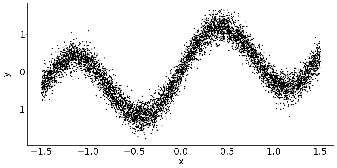
(a) sin normal

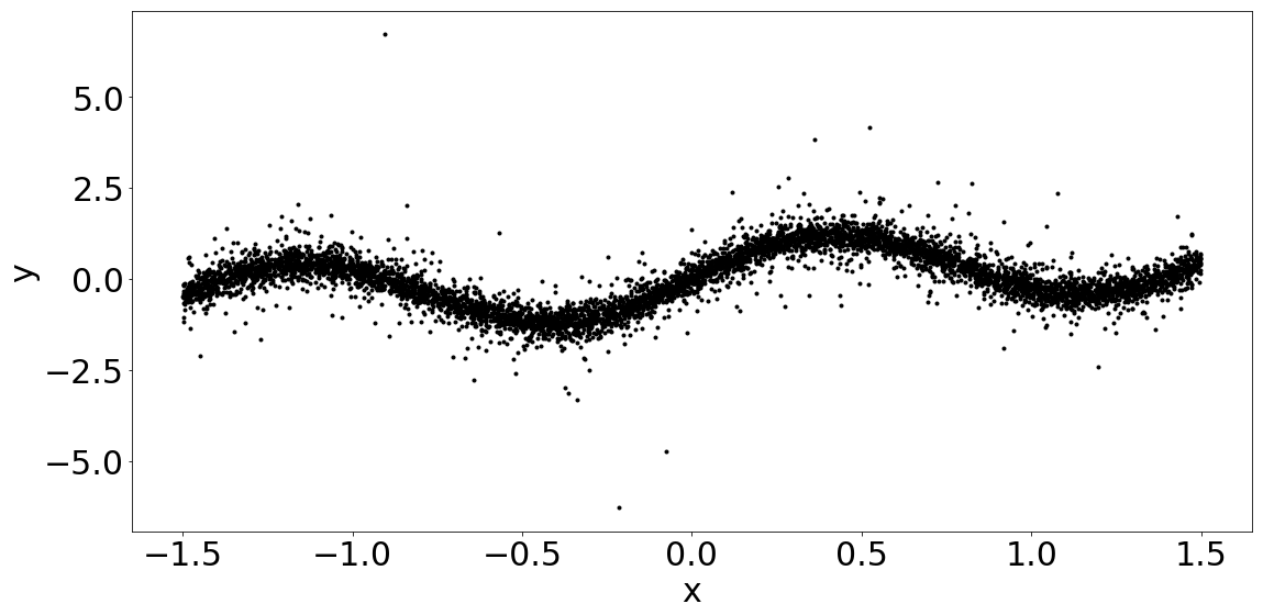
(b) sin t

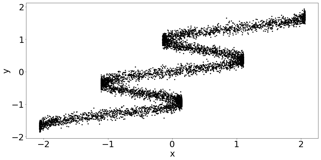
(c) inv sin normal

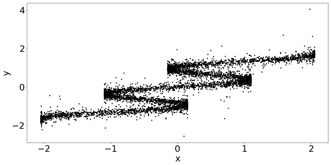
(d) inv sin t

Figure S5: Generated Univariate Response Data.

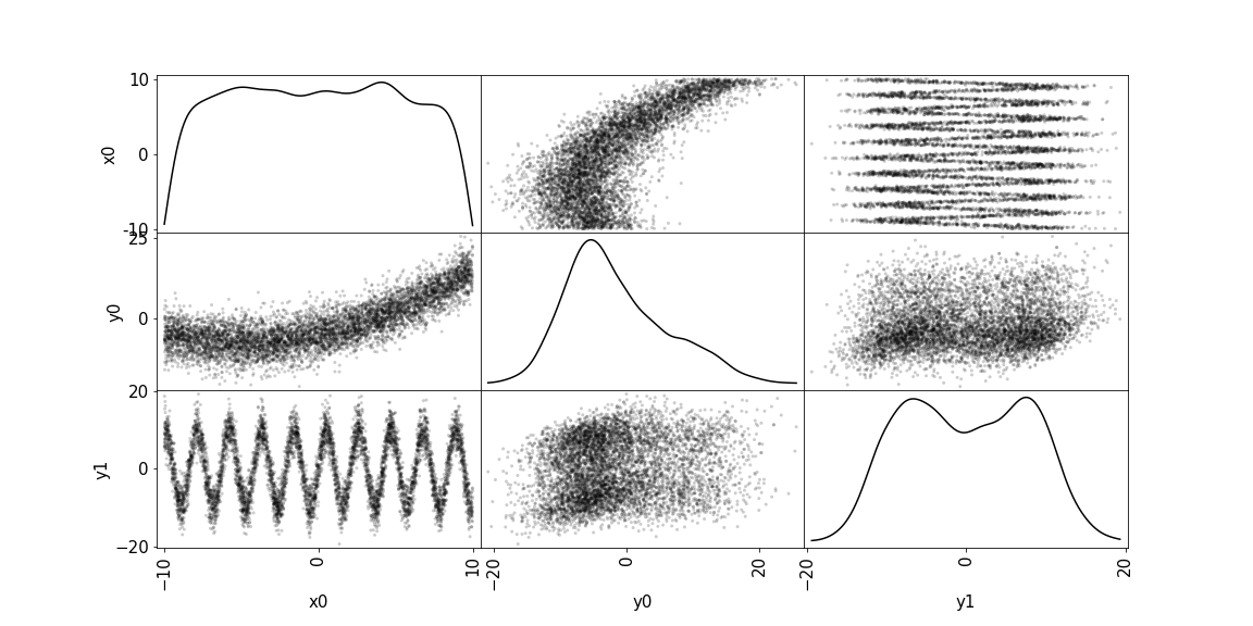
Figure S6: Generated Multivariate Response Data.

Fitting the data by conditional mean models, such as a regular neural network with mean squared error, is not suitable in the case when we deal with multimodal output. In this case, we should be using models that can encode the probabilistic structure of the data. We show in Figure S7 that proposed and baseline models can capture the multimodality correctly.

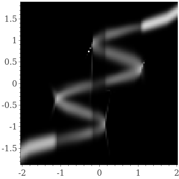
(a) RNADE N

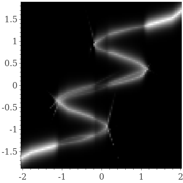
(b) RNADE L

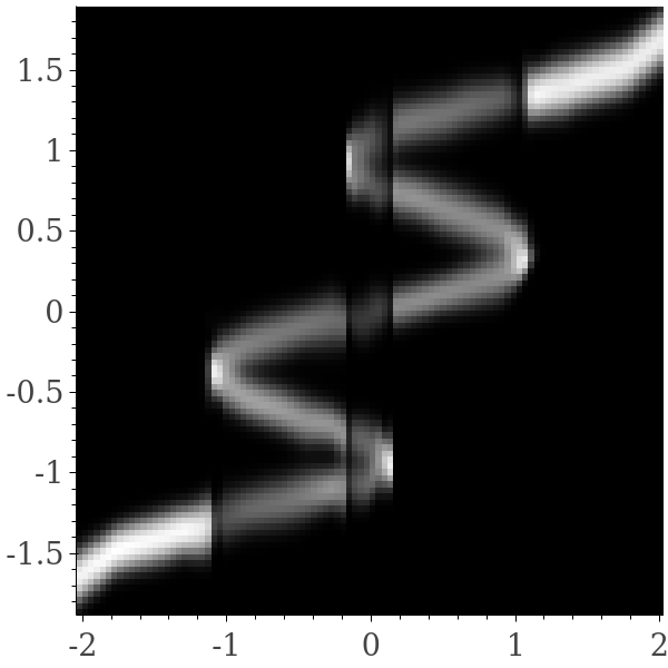
(c) RNADE DEEP N

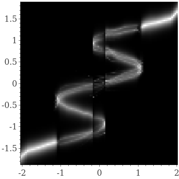
(d) RNADE DEEP L

(e) MDN

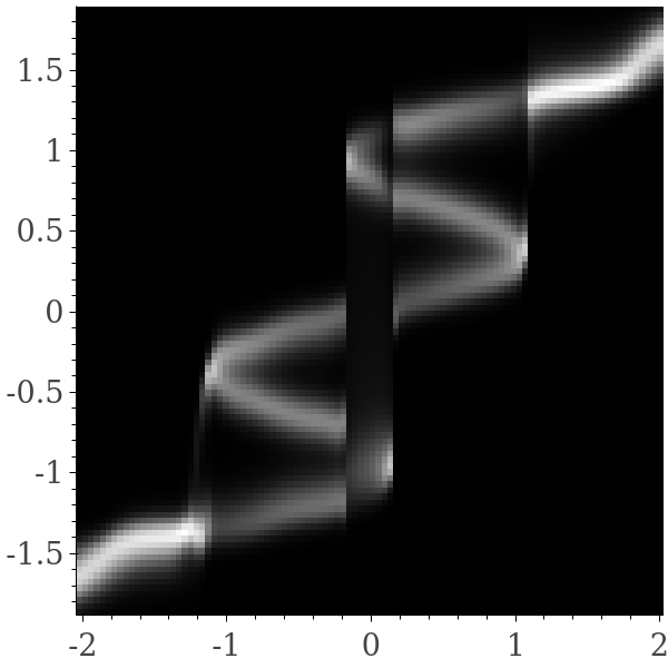
(f) MONDE

Figure S7: Density Heatmap - Inv Sin Normal.

In Figure S8, we show density heatmaps computed from different density estimators and data generating processes. In these plots, we show density $f(y_{0},y_{1}=0~{}|~{}x)$ of baseline and proposed models for a grid of points spanned over $y_{0}$ and $x$. We see that RNADE and MDN models have difficulty in encoding the probabilistic structure, but our models can capture it well, which is also confirmed by the test log-likelihood evaluations shown in Table 2.

(a) Gen Distribution

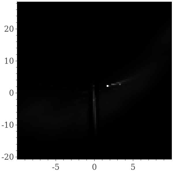
(b) RNADE N

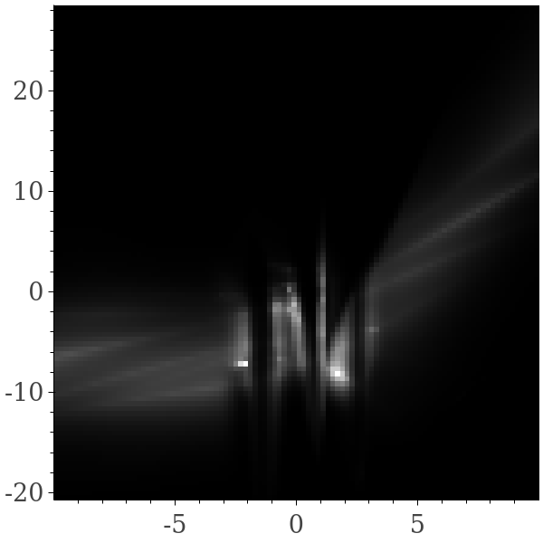
(c) RNADE L

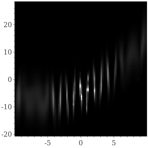
(d) RNADE DEEP N

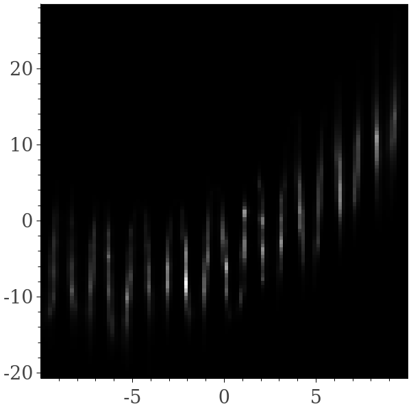
(e) RNADE DEEP L

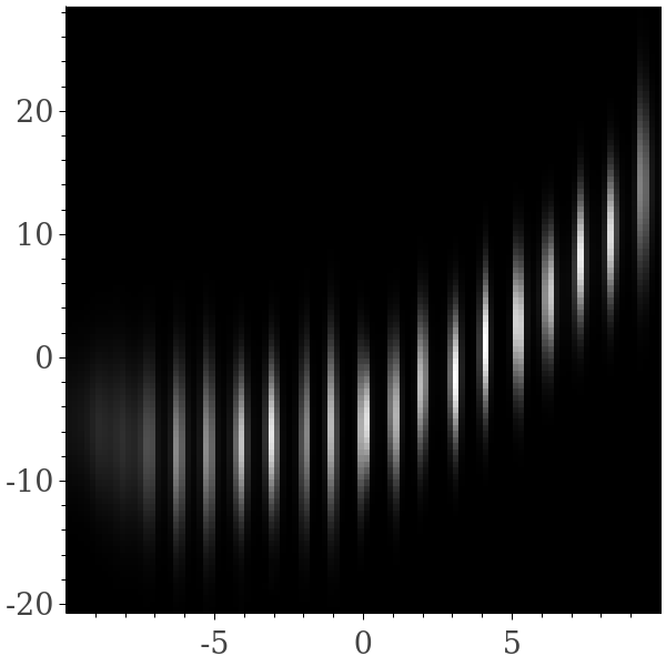
(f) MDN Const Cov

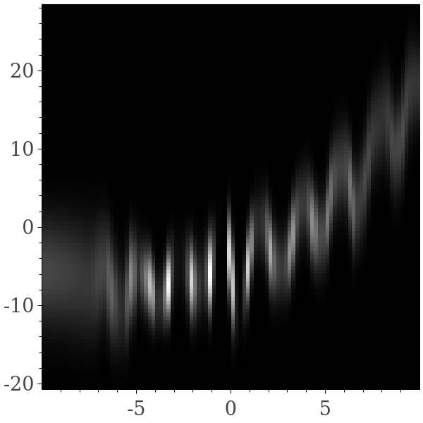
(g) MDN Param Cov

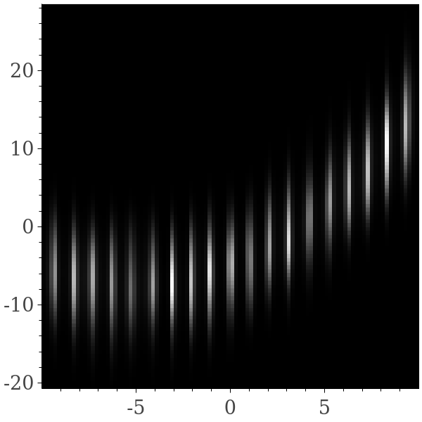
(h) MONDE Const Cov

(i) MONDE Param Cov

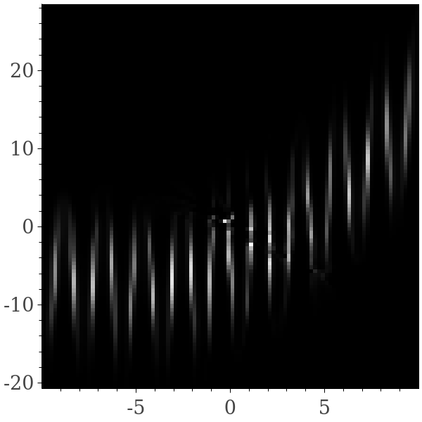
(j) MONDE AR

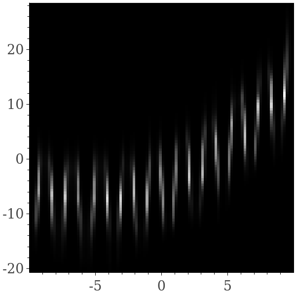
(k) PUMONDE

Figure S8: Density Heatmap ($f(y_{0},y_{1}=0~{}|~{}x)$) - MV Nonlinear.

S4.4 SMALL UCI DATASETS

Table 3: Mean Loglikelihoods - Small UCI Datasets.

	RNADE Laplace	RNADE Normal	RNADE Deep Normal	RNADE Deep Laplace	MONDE Const Cov	MONDE Param Cov	MONDE AR	PUMONDE	MDN
UCI Redwine 2D	-2.543	-2.506	-3.310	-2.343	-2.672	-2.462	-1.795	-1.997	-2.250
UCI Redwine Unsupervised	-6.574	-6.496	-8.244	-8.297	-2.992	-1.879	-8.077		-8.676
UCI Whitewine 2D	-1.958	-1.956	-1.957	-1.968	-1.910	-1.891	-1.915	-1.901	-1.940
UCI Parkinsons 2D	-1.406	-1.323	-1.424	-2.910	-4.032	-4.766	-1.134	-1.254	-1.368
UCI Parkinsons Unsupervised	0.999	0.304	-3.265	-3.214	1.328	-3.654	3.055		-0.870

The results from the experiments using smaller UCI datasets (Dua and Graff, 2019) are shown in Table 3. The UCI datasets are preprocessed in the same way as done by Uria et al. (2013) i.e., we removed categorical variables and variables which have absolute value of Pearson coefficient correlation with other variable larger than 0.98. We use each UCI dataset in two separate experiments. Firstly, by assuming the two last columns as response variables (ordering as defined by the documentation of the data), while the remaining columns constitute the covariates. These are the datasets with suffix “2D”. Secondly, we perform experiments by using all columns as response variables, hence assuming the covariate vector is empty. These datasets are given the suffix “unsupervised”.

MONDE models achieve the best results among all model trained in these datasets.

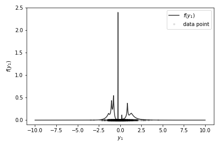
(a) RNADE

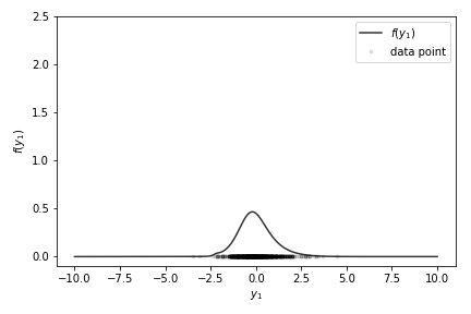
(b) MONDE

Figure S9: Densities estimated by the RNADE and MONDE AR models for the first variable in AR ordering when the corresponding variable had a small number of values. The data points are also shown on the $x$ axis as black dots.

We report that when we trained the models on datasets composed solely of continuous variables where some columns have a considerably small number of unique values (but still specified as real type variables by the dataset documentation), the RNADE models tend to “overfit” by placing very narrow Gaussians at particular points (the test likelihood is high, but this is an artefact of treating essentially discrete data as if it had a density). This was especially a problem for RNADE model, when one of such problematic variables was the first variable in the autoregressive expansion for the joint probability. In this case, because train, validation and test data contained a lot of points with the same values, RNADE could create overfitted first unconditional densities. This is not a realistic training procedure, since the data here is discrete for all practical purposes, resulting on unbounded test “densities” being easily achieved depending on the minimal scale allowed for a Gaussian mixture component in the training procedure. In Figure S9, we show an example of the $f(y_{1})$ density estimated by the RNADE model using a mixture of Laplace distributions, and the density of the same variable estimated by the autoregressive MONDE model. The data is the UCI whitewine dataset (used as an unsupervised case i.e. all variables treated as response variables with covariate set being empty). We checked that MONDE models were not impacted by this spurious “continuous” variables and fitted smooth distributions. In our final experiment runs, we imposed the rule to remove a column if it has below 5% of unique values, compared to the number of samples. Only when we removed such columns we were able to train the RNADE models to the satisfactory level of generalization.

S4.5 FINANCIAL DATASETS

Table 4: Mean Loglikelihoods - Financial Datasets.

	RNADE Laplace	RNADE Normal	RNADE Deep Normal	RNADE Deep Laplace	MONDE Const Cov	MONDE Param Cov	MONDE AR	PUMONDE	MDN
ETF 1D	-1.416	-1.495	-1.422	-1.408	-1.383			-1.398
ETF 2D	-1.501	-1.472	-1.857	-1.588	-1.426	-1.466	-1.401	-1.599	-1.441
FX EUR Predicted	-1.054	-1.074	-1.093	-1.272	-1.081			-1.185
FX EUR GBP Predicted	-2.070	-2.072	-2.268	-2.024	-2.292	-2.162	-2.074	-2.048	-2.130
FX ALL Predicted	-2.940	-2.985	-3.479	-3.741	-4.853	-8.107	-2.838		-5.604

The results from experiments with financial datasets are shown in Table 4. We use two different sources of the financial data.

The first source is the the Yahoo service from which we downloaded exchange traded funds dataset. We obtain two time series of daily close prices between dates: 03.01.2011 and 14.04.2015. The “ETF 1D” are daily returns of the SPY financial instrument. The response and covariate variables in this dataset are consecutive returns in the time series accordingly. The “ETF 2D” are daily returns of the SPY and DIA symbols. The returns are aggregated into the final dataset using the same transformation as in the fist univariate case, but this time both instrument returns are combined together so response and covariate vectors have two components.

The second source is the FXCM repository from which we downloaded the foreign exchange tick data. We downloaded prices for the following currency pairs: EURUSD, GBPUSD, USDJPY, USDCHF, USDCAD, NZDUSD, NZDJPY, GBPJPY for the period between 05.01.2015 and 30.01.2015. Each currency pair dataset contains top of the book tick level bid and offer prices. We computed the returns of the mid point prices for these time series. Then we subsumpled each time series using a 1 minute interval and aligned all of them into one data frame. This table of aligned currency pairs’ returns was used to create three datasets. “FX EUR predicted” contains the EURUSD returns as the response variable and ten previous historical returns from all currency pairs as covariates i.e. if we have EURUSD return at time $t$, we collected for this response covariates as returns for all instruments at times $t-1,t-2,\ldots,t-10$. The “FX EUR and GBP predicted” dataset was constructed as the previous one but with two response variables i.e. EURUSD and GBPUSD returns and the covariates constructed from all four previous historical returns plus hour of day variable. The “FX all assets predicted” dataset contains all contemporaneous currency pairs returns as response and two autoregressive returns of all currency pairs as covariates. We see from the results in Table 4 that there is an improvement in using our approach in an autoregressive representation and other versions of our model are also comparable with recently proposed solutions.

S4.5.1 Classification

In Section 4.2 we used the following foreign exchange instruments to construct the experiment dataset: AUDCAD, AUDJPY, AUDNZD, EURCHF, NZDCAD, NZDJPY, NZDUSD, USDCHF, USDJPY, EURUSD, GBPUSD and USDCAD.

S4.5.2 Bivariate likelihood

In Section 4.5 we used the following foreign exchange instruments to construct the experiment dataset: AUDCAD, AUDJPY, AUDNZD, AUDCHF, EURAUD, EURCHF, NZDCAD, CADCHF, EURJPY, NZDJPY, GBPNZD, GBPJPY, NZDUSD, USDCHF, GBPCHF, USDJPY, EURUSD, GBPUSD, EURGBP, USDCAD and NZDCHF.

S4.6 TAIL DEPENDENCE

To compute tail dependence, we use empirical functions suggested by (Charpentier, 2012) and (Venter and Instrat, 2001):

$$\hat{\lambda}_{L}(u) =\frac{\sum_{k=1}^{n}\mathbf{1}(Y_{i,k}\leq\hat{F}_{i}^{-1}(u),Y_{j,k}\leq\hat{F}_{j}^{-1}(u))}{\sum_{k=1}^{n}\mathbf{1}(Y_{i,k}\leq\hat{F}_{i}^{-1}(u))}$$ (S1)

$$\hat{\lambda}_{R}(u) =\frac{\sum_{k=1}^{n}\mathbf{1}(Y_{i,k}>\hat{F}_{i}^{-1}(u),Y_{j,k}>\hat{F}_{j}^{-1}(u))}{\sum_{k=1}^{n}\mathbf{1}(Y_{i,k}>\hat{F}_{i}^{-1}(u))},$$ (S2)

for the models where it is possible to directly sample new data (like MAF and MDN), and for datasets used for training generated from the mixture model. We plug-in the distribution transformation $\hat{F}_{i}(y_{i,k})$ computed directly from sampled data using the rank function.

To compute tail dependence indices for models which we cannot sample new data easily but we can compute marginal distribution functions (like PUMONDE, MONDE Copula) we apply the following process: 1) Estimate the marginal quantile functions numerically conditioning it on the mean of one of the mixtures: $\hat{F}_{i}^{-1}(\cdot|mean(\mathbf{x}_{c}))$; 2) Generate vector $\mathbf{u}$ as a grid of points equidistantly spaced between $(0,1)$ (we use the same grid $\mathbf{u}$ used for computing tail indices for models that are easy to sample from); 3) Compute $\hat{F}_{k}^{-1}(\mathbf{u}|mean(\mathbf{x}_{c}))$ for $k=i,j$ 4) Compute $\hat{F}_{ij}(\hat{F}_{i}^{-1}(\mathbf{u}|mean(\mathbf{x}_{c}),\hat{F}_{j}^{-1}(\mathbf{u}|mean(\mathbf{x}_{c}))|mean(\mathbf{x}_{c}))$ directly from the model and substitute it into the $\lambda_{L}(u)$ and $\lambda_{R}(u)$ equations from Section 4.3.

S5 SOURCE CODE

Source code is provided in https://github.com/pawelc/NeuralLikelihoods.

Table 5: Hyper parameters search space

EXPERIMENT	MODEL	SEARCH SPACE	DATA SET/BEST PARAMETERS
Synthetic Data, Small UCI Data, Financial Data	RNADE Normal	hidden units $\in(20,200)$ number of components in mixture $\in(1,100)$ learning rate $\in(10^{-4},10^{-2})$ batch size $=200$	Sin Normal (30;93;0.0044) Sin T (90;7;0.0017) Inv Sin Normal (69;7;0.0022) Inv Sin T (69;7;0.0022) MV Nonlinear (194;100;0.0089) UCI Redwine 2D (170;50;0.001) UCI Redwine Unsupervised (164;10;0.0011) UCI Whitewine 2D (100;24;0.0012) UCI Whitewine Unsupervised (56;30;0.0002) UCI Parkinsons 2D (104;11;0.0064) UCI Parkinson Unsupervised (200;24;0.0006) ETF 1D (69;7;0.0022) ETF 2D (164;1;0.0041) FX EUR Predicted (176;83;0.0046) FX EUR GBP Predicted (189;78;0.0027) FX All predicted (69;7;0.0022)
Synthetic Data, Small UCI Data, Financial Data	RNADE Laplace	hidden units $\in(20,200)$ number of components in mixture $\in(1,100)$ learning rate $\in(10^{-4},10^{-2})$ batch size $=200$	Sin Normal (100;24;0.0012) Sin T (56;30;0.0002) Inv Sin Normal (172;32;0.0011) Inv Sin T (200;67;0.0046) MV Nonlinear (90;67;0.0074) UCI Redwine 2D (20;100;0.0065) UCI Redwine Unsupervised (69;7;0.0022) UCI Whitewine 2D (69;7;0.0022) UCI Whitewine Unsupervised (100;24;0.0012) UCI Parkinsons 2D (90;67;0.0074) UCI Parkinson Unsupervised (138;25;0.0021) ETF 1D (200;1;0.01) ETF 2D (200;1;0.01) FX EUR Predicted (47;5;0.0017) FX EUR GBP Predicted (146;7;0.0011) FX All predicted (69;7;0.0022)
Synthetic Data, Small UCI Data, Financial Data	MONDE Const Cov	number of layers for x transformation $\in(0,3)$ number of hidden units per layer for x transformation $\in(10,200)$ number of layers y transformation $\in(1,5)$ number of hidden units per layer for y transformation $\in(10,200)$ learning rate $\in(10^{-4},10^{-2}$ batch size $=200$	Sin Normal (1;131;4;10;0.0016) Sin T (1;112;2;110;0.0008) Inv Sin Normal (0;0;2;126;0.0004) Inv Sin T (1;112;2;110;0.0008) MV Nonlinear (3;113;1;89;0.0002) UCI Redwine 2D (0;0;4;10;0.0001) UCI Redwine Unsupervised (0;0;2;65;0.0002) UCI Whitewine 2D (0;0;3;28;0.0064) UCI Whitewine Unsupervised (0;0;3;200;0.0001) UCI Parkinsons 2D (1;112;2;110;0.0008) UCI Parkinson Unsupervised (0;0;1;10;0.0005) ETF 1D (3;200;1;200;0.0001) ETF 2D (0;0;1;200;0.0003) FX EUR Predicted (0;0;1;10;0.0001) FX EUR GBP Predicted (2;10;4;10;0.01) FX All predicted (0;0;5;200;0.0039)
Synthetic Data, Small UCI Data, Financial Data	MONDE Param Cov	number of layers for x transformation $\in(0,3)$ number of hidden units per layer for x transformation $\in(10,200)$ number of layers y transformation $\in(1,5)$ number of hidden units per layer for y transformation $\in(10,200)$ number of layers for x covariance transformation $\in(1,3)$ number of hidden units per layer for x covariance transformation $\in(10,200)$ learning rate $\in(10^{-4},10^{-2}$ batch size $=200$	MV Nonlinear (3;200;4;116;0;0;0.0003) UCI Redwine 2D (0;0;2;200;0;0;0.01) UCI Redwine Unsupervised (0;0;2;65;0;0;0.0002) UCI Whitewine 2D (2;17;2;35;2;79;0.0068) UCI Whitewine Unsupervised (0;0;4;69;0;0;0.0001) UCI Parkinsons 2D (1;121;1;184;0;0;0.0066) UCI Parkinson Unsupervised (0;0;4;70;0;0;0.0011) ETF 2D (1;54;3;127;?;?;0.0081) FX EUR GBP Predicted (0;0;5;10;?;?;0.0001) FX All predicted (1;68;3;191;?;?;0.01)
Synthetic Data, Small UCI Data, Financial Data	MDN	number of hidden layers $\in(1,6)$ number of hidden units per layer $\in(20,200)$ number of components in mixture $\in(1,100)$ learning rate $\in(10^{-4},10^{-2}$ batch size $=200$	Sin Normal (6;20;1;0.0001) Sin T (4;74;45;0.0003) Inv Sin Normal (2;82;95;0.0034) Inv Sin T (1;141;60;0.0022) MV Nonlinear (3;61;54;0.0067) UCI Redwine 2D (6;20;100;0.0002) UCI Redwine Unsupervised (6;188;14;0.0099) UCI Whitewine 2D (4;74;45;0.0003) UCI Whitewine Unsupervised (6;20;100;0.01) UCI Parkinsons 2D (1;104;11;0.0064) UCI Parkinson Unsupervised (6;94;98;0.0026) ETF 1D (2;114;9;0.0068) ETF 2D (2;114;9;0.0068) FX EUR Predicted (1;24;99;0.0001) FX EUR GBP Predicted (6;172;32;0.0011) FX All predicted (6;181;59;0.0011)
Synthetic Data, Small UCI Data, Financial Data	MONDE AR	number of hidden layers for x transformation $\in(0,3)$ number of hidden units per x transformation layer $\in(10,200)$ number of hidden layers for y transformation $\in(1,5)$ number of hidden units per y transformation layer $\in(10,200)$ learning rate $\in(10^{-4},10^{-2}$ batch size $=200$	MV Nonlinear (1;22;1;180;0.0001) UCI Redwine 2D (0;0;3;28;0.0064) UCI Redwine Unsupervised (0;0;1;37;0.0038) UCI Whitewine 2D (0;0;2;159;0.0007) UCI Whitewine Unsupervised (0;0;2;10;0.0036) UCI Parkinsons 2D (1;121;1;184;0.0066) UCI Parkinson Unsupervised (1;130;1;199;0.0064) ETF 1D ETF 2D (0;0;1;176;0.01) FX EUR GBP Predicted (0;0;5;10;0.01) FX All predicted (0;0;3;28;0.0064)
Synthetic Data, Small UCI Data, Financial Data	PUMONDE	number of hidden layers for x transformation $\in(1,3)$ number of hidden units per x transformation layer $\in(10,200)$ number of hidden layers for y transformation $\in(1,3)$ number of hidden units per y transformation layer $\in(10,200)$ number of hidden layers for xy transformation $\in(1,3)$ number of hidden units per xy transformation layer $\in(10,200)$ learning rate $\in(10^{-4},10^{-3}$ batch size $=200$	MV Nonlinear (0;0;3;67;2;118;0.0002) UCI Redwine 2D (1;37;3;88;1;129;0.0007) UCI Redwine Unsupervised UCI Whitewine 2D (2;17;2;35;2;79;0.0068) UCI Parkinsons 2D (2;117;2;35;2;79;0.0068) ETF 2D (0;0;3;67;2;118;0.0002) FX EUR GBP Predicted (0;0;3;67;2;118;0.0002)
Density Estimation	MONDE MADE	number of hidden layers $\in\{8,10\}$ number of blocks $\in\{40,60\}$ start batch size $=128$ batch size increments $=3$ learning rate $=0.001$	Power (10;40)
Density Estimation	MONDE MADE	number of hidden layers $\in\{8,10\}$ number of blocks $\in\{60,80\}$ start batch size $=128$ batch size increments $=5$ learning rate $=0.001$	Gas (10;80) Hepmass (8;60)
Density Estimation	MONDE MADE	number of hidden layers $\in\{3,5,7,8\}$ number of blocks $\in\{10,50,80\}$ start batch size $=128$ batch size increments $=5$ batch size increase patience threshold = $=20$ learning rate $=0.001$	Miniboone (5;10)
Density Estimation	MONDE MADE	number of hidden layers $\in\{3,5,7\}$ number of blocks $\in\{10,30,40\}$ start batch size $=128$ batch size increments $=3$ batch size increase patience threshold = $=20$ learning rate $=0.001$	Bsds300 (3;10)
Classification	MONDE Const Cov	number of layers for x transformation $\in\{2,4\}$ number of hidden units per layer for x transformation $\in\{50,100\}$ number of layers y transformation $\in\{2,4\}$ number of hidden units per layer for y transformation $\in\{50,100\}$ number of hidden units per layer in y transformation used for x,y transformation $=30$ covariance learning rate $=0.05$ start batch size $=128$ batch size increments $=3$ batch size increase patience threshold = $=20$ learning rate $=0.001$	Classification (FX) (2;100;4;100)
Classification	MONDE Param Cov	number of layers for x transformation $\in\{2,4\}$ number of hidden units per layer for x transformation $\in\{50,100\}$ number of layers y transformation $\in\{2,4\}$ number of hidden units per layer for y transformation $\in\{50,100\}$ number of layers used for covariance parametrization $\in\{2,4\}$ number of hidden units per layer in covariance parametrization $\in\{50,100\}$ number of hidden units per layer in y transformation used for x,y transformation $=30$ start batch size $=128$ batch size increments $=3$ batch size increase patience threshold = $=20$ learning rate $=0.001$	Classification (FX) (2;100;4;50;2;100)
Classification	PUMONDE	number of layers for x transformation $\in\{3,4\}$ number of hidden units per layer for x transformation $\in\{50,100\}$ number of layers for y transformation $\in\{3,4\}$ number of hidden units per layer for y transformation $\in\{50,100\}$ number of layers for x,y transformation $\in\{3,4\}$ number of hidden units per layer for x,y transformation $\in\{50,100\}$ number of hidden units per layer in y transformation used for x,y transformation $=30$ start batch size $=128$ batch size increments $=3$ batch size increase patience threshold = $=20$ learning rate $=0.001$	Classification (FX) (3;50;4;50;4;50)
Classification	NN Classifier	number of layers $\in\{2,3,5\}$ number of hidden units per layer$\in\{50,100\}$ start batch size $=128$ batch size increments $=3$ batch size increase patience threshold = $=20$ learning rate $=0.001$	Classification (FX) (3;100)
Classification	Random Forest	number of estimators $\in\{10,50,100\}$ maximum tree depth $\in\{5,10,20\}$	Classification (FX) (100;20)
Classification	Xgb Classifier	subsample $\in\{0.1,0.2,0.3,0.4,0.5,0.6,0.7,0.8,1.0\}$	Classification (FX) (0.3)
Tail Dependence Mutual Information	MONDE Const Cov	number of layers for x transformation $\in\{3,4\}$ number of hidden units per layer for x transformation $\in\{50,100\}$ number of layers y transformation $\in\{3,4\}$ number of hidden units per layer for y transformation $\in\{50,100\}$ number of hidden units per layer in y transformation used for x,y transformation $=30$ covariance learning rate $=0.05$ start batch size $=128$ batch size increments $=3$ batch size increase patience threshold = $=20$ learning rate $=0.001$	Mixture Process (3;100;3;50)
Tail Dependence Mutual Information	MONDE Param Cov	number of layers for x transformation $\in\{3,4\}$ number of hidden units per layer for x transformation $\in\{50,100\}$ number of layers y transformation $\in\{3,4\}$ number of hidden units per layer for y transformation $\in\{50,100\}$ number of layers used for covariance parametrization $\in\{3,4\}$ number of hidden units per layer in covariance parametrization $\in\{50,100\}$ number of hidden units per layer in y transformation used for x,y transformation $=30$ start batch size $=128$ batch size increments $=3$ batch size increase patience threshold = $=20$ learning rate $=0.001$	Mixture Process (3;50;3;50;4;50)
Tail Dependence Mutual Information	PUMONDE	number of layers for x transformation $\in\{3,4\}$ number of hidden units per layer for x transformation $\in\{50,100\}$ number of layers for y transformation $\in\{3,4\}$ number of hidden units per layer for y transformation $\in\{50,100\}$ number of layers for x,y transformation $\in\{3,4\}$ number of hidden units per layer for x,y transformation $\in\{50,100\}$ number of hidden units per layer in y transformation used for x,y transformation $=30$ start batch size $=128$ batch size increments $=3$ batch size increase patience threshold = $=20$ learning rate $=0.001$	Mixture Process (3;100;3;100;4;100)
Tail Dependence Mutual Information	MAF	number of bijectors $\in\{2,4,5,8\}$ number of layers in each bijector $\in\{1,2,4\}$ number of hidden units per layer in bijector $\in\{64,128,512\}$ number of hidden units for covariate transformation $\in\{16,32,64\}$ batch normalization $\in\{True,False\}$ learning rate $\in\{1e^{-3},1e^{-4}\}$ batch size $=128$	Mixture Process (5;1;512;16;True;0.001)
Tail Dependence Mutual Information	MDN	number of hidden layers $\in(2,3,5)$ number of hidden units per layer $\in(128,512)$ number of components in mixture $\in(2,10,50,100)$ learning rate $\in\{1e^{-3},1e^{-4}\}$ batch size $=128$	Mixture Process (5;128;100;0.001)
Bivariate Likelihood	MONDE Const Cov	number of layers for x transformation $\in\{2,4\}$ number of hidden units per layer for x transformation $\in\{50,100\}$ number of layers y transformation $\in\{2,4\}$ number of hidden units per layer for y transformation $\in\{50,100\}$ number of hidden units per layer in y transformation used for x,y transformation $=30$ covariance learning rate $=0.05$ start batch size $=128$ batch size increments $=3$ batch size increase patience threshold = $=20$ learning rate $=0.001$	FX (2;50;2;50)
Bivariate Likelihood	MONDE Param Cov	number of layers for x transformation $\in\{2,4\}$ number of hidden units per layer for x transformation $\in\{50,100\}$ number of layers y transformation $\in\{2,4\}$ number of hidden units per layer for y transformation $\in\{50,100\}$ number of layers used for covariance parametrization $\in\{2,4\}$ number of hidden units per layer in covariance parametrization $\in\{50,100\}$ number of hidden units per layer in y transformation used for x,y transformation $=30$ start batch size $=128$ batch size increments $=3$ batch size increase patience threshold = $=20$ learning rate $=0.001$	FX (2;50;4;100;2;100)
Bivariate Likelihood	PUMONDE	number of layers for x transformation $\in\{2,3\}$ number of hidden units per layer for x transformation $\in\{128,256\}$ number of layers for y transformation $\in\{2,3\}$ number of hidden units per layer for y transformation $\in\{64,128\}$ number of layers for x,y transformation $\in\{2,3\}$ number of hidden units per layer for x,y transformation $\in\{64,128\}$ number of hidden units per layer in y transformation used for x,y transformation $=16$ batch size $=128$ learning rate $=0.001$	FX (2;128;3;128;3;64)
Bivariate Likelihood	MDN	number of hidden layers $\in(2,3,5)$ number of hidden units per layer $\in(128,512)$ number of components in mixture $\in(2,10,50,100)$ learning rate $\in\{1e^{-3},1e^{-4}\}$ batch size $=128$	FX (2;512;2;0.0001)

References

- Bishop (1994) C. Bishop. Mixture density networks. Technical report, NCRG 4288, Aston University, Birmingham, 1994.
- Charpentier (2012) A. Charpentier. Copulas and tail dependence, part 1. https://freakonometrics.hypotheses.org/2435, 2012. Accessed: 2019-12-28.
- Chen and Guestrin (2016) T. Chen and C. Guestrin. XGBoost: A scalable tree boosting system. In KDD, 2016.
- De Cao and Titov (2019) N. De Cao and I. Titov. Block neural autoregressive flow. In UAI, 2019.
- Diederik and Jimmy (2015) K. Diederik and B. Jimmy. Adam: A method for stochastic optimization. In ICLR, 2015.
- Dinh et al. (2015) L. Dinh, D. Krueger, and Y. Bengio. NICE: Non-linear independent components estimation. In ICLR, 2015.
- Dinh et al. (2017) L. Dinh, J. Sohl-Dickstein, and S. Bengio. Density estimation using Real NVP. In ICLR, 2017.
- Dua and Graff (2019) D. Dua and C. Graff. UCI machine learning repository, 2019. URL http://archive.ics.uci.edu/ml.
- Elidan (2013) G. Elidan. Copulas in machine learning. In Copulae in Mathematical and Quantitative Finance. Springer, Berlin, 2013.
- Germain et al. (2015) M. Germain, K. Gregor, I. Murray, and H. Larochelle. MADE: Masked autoencoder for distribution estimation. In ICML, 2015.
- Holton (2003) G.A. Holton. Value-at-risk: Theory and Practice. Academic Press Inc, 2003.
- Huang et al. (2018) C-W. Huang, D. Krueger, A. Lacoste, and A. Courville. Neural autoregressive flows. In ICML, 2018.
- Huang and Frey (2008) J. Huang and B. Frey. Cumulative distribution networks and the derivative-sum-product algorithm. In UAI, 2008.
- Huang et al. (2010) J. Huang, N. Jojic, and C. Meek. Exact inference and learning for cumulative distribution func- tions on loopy graphs. In NIPS, 2010.
- Ioffe and Szegedy (2015) S. Ioffe and C. Szegedy. Batch normalization: Accelerating deep network training by reducing internal covariate shift. In ICML, 2015.
- Joe (1997) H. Joe. Multivariate models and dependence concepts. Monographs on statistics and applied probability. CRC Press, 1997.
- Jordan and Jacobs (1994) M. Jordan and R. Jacobs. Hierarchical mixtures of experts and the EM algorithm. Neural Computation, 6:181–214, 1994.
- Lang (2005) B. Lang. Monotonic multi-layer perceptron networks as universal approximators. In ICANN, 2005.
- Larochelle and Murray (2011) H. Larochelle and I. Murray. The neural autoregressive distribution estimator. In AISTATS, 2011.
- Liew et al. (2016) S. Liew, M. Khalil-Hani, and R. Bakhteri. Bounded activation functions for enhanced training stability of deep neural networks on visual pattern recognition problems. Neurocomputing, 216, 2016.
- Likas (2001) A. Likas. Probability density estimation using artificial neural networks. Computer Physics Communications, 135(2), 2001.
- Magdon-Ismail et al. (2002) M. Magdon-Ismail, , and A. Atiya. Density estimation and random variate generation using multilayer networks. IEEE Trans. Neural Networks, 13(3), 2002.
- Minin et al. (2010) A. Minin, M. Velikova, B. Lang, and H. Daniels. Comparison of universal approximators incorporating partial monotonicity by structure. Neural Networks, 23(4), 2010.
- Minka (2019) T. Minka. From automatic differentiation to message passing. Invited talk at the Advances and challenges in Machine Learning Languages workshop (ACMLL 2019), 2019. URL https://tminka.github.io/papers/acmll2019/.
- Oliva et al. (2018) J. Oliva, A. Dubey, M. Zaheer, B. Póczos, R. Salakhutdinov, E. Xing, and J. Schneider. Transformation autoregressive networks. In ICML, 2018.
- Papamakarios et al. (2017) G. Papamakarios, T. Pavlakou, and I. Murray. Masked autoregressive flow for density estimation. In NIPS, 2017.
- Rapisarda et al. (2007) F. Rapisarda, D. Brigo, and F. Mercurio. Parameterizing correlations: a geometric interpretation. IMA Journal of Management Mathematics, 18(1), 2007.
- Schmidt (2006) T. Schmidt. Coping with copulas. In Copulas – From Theory to Applications in Finance, pages 3–34. Risk Books, 2006.
- Sill (1997) J. Sill. Monotonic networks. In NIPS, 1997.
- Sill and Abu-Mostafa (1996) J. Sill and Y. Abu-Mostafa. Monotonicity hints. In NIPS, 1996.
- Silva (2015) R. Silva. Bayesian inference in cumulative distribution fields. Interdisciplinary Bayesian Statistics, pages 83–95, 2015.
- Silva et al. (2011) R. Silva, C. Blundell, and Y-W. Teh. Mixed cumulative distribution networks. In AISTATS, 2011.
- Sklar (1959) A. Sklar. Fonctions de répartition à n dimensions et leurs marges. Publications de l’Institut de Statistique de l’Université de Paris, 8, 1959.
- Smith et al. (2018) S. Smith, P-J. Kindermans, C. Ying, and V. Le Quoc. Don’t decay the learning rate, increase the batch size. In ICLR, 2018.
- Trentin (2016) E. Trentin. Soft-constrained nonparametric density estimation with artificial neural networks. In ANNPR, 2016.
- Uria et al. (2013) B. Uria, I. Murray, and H. Larochelle. RNADE: the real-valued neural autoregressive density-estimator. In NIPS, 2013.
- Uria et al. (2014) B. Uria, I. Murray, and H. Larochelle. A deep and tractable density estimator. In ICML, 2014.
- Varin et al. (2011) C. Varin, N. Reid, and D. Firth. An overview of composite likelihood methods. Statistica Sinica, 21(1), 2011.
- Venter and Instrat (2001) G. Venter and G. Instrat. Tails of copula. In ASTIN, 2001.
- Wang (1994) S. Wang. A neural network method of density estimation for univariate unimodal data. NCAA, 2(3), 1994.
- Zhang (2018) S. Zhang. From CDF to PDF — A density estimation method for high dimensional data. arXiv:1804.05316, 2018.