Describing dynamics of driven multistable oscillators with phase transfer curves

Abstract

Phase response curve is an important tool in studies of stable self-sustained oscillations; it describes a phase shift under action of an external perturbation. We consider multistable oscillators with several stable limit cycles. Under a perturbation, transitions from one oscillating mode to another one may occur. We define phase transfer curves to describe the phase shifts at such transitions. This allows for a construction of one-dimensional maps that characterize periodically kicked multistable oscillators. We show, that these maps are good approximations of the full dynamics for large periods of forcing.

For many practical applications it is important to know how oscillators respond to perturbations. If the oscillator is stable, after a perturbation it returns to its oscillating mode, only the phase is shifted. This is quantified by a phase response curve, which is an important tool to study dynamics of forced and coupled oscillators. Quite often there exist several stable oscillating modes, one speaks in this case on multistability. For multistable oscillators, external action may result in a switching from one mode to another one. We extend the concept of phase response curve on this case by introducing a phase transfer curve, describing dependence of the phase of the target mode on the phase of the source one.

I Introduction

The concept of phase response curves (PRC) is widely used in the theory of oscillations to describe sensitivity of limit cycle oscillations to external actions [1; 2; 3]. Moreover, because PRCs can be rather easy measured in experiments, they find broad applications in studies of oscillating processes in life systems, where equations for the oscillators are hardly available, see e.g. [4; 5; 6; 7; 8; 9; 10; 11]. The form of the PRC is important for controlling the oscillator by external forcing [12; 13; 14]. One of practical applications is optimal re-adjustment of the phase of circadian rhythms of humans [15]. Here, the concept of PRC (sometimes one speaks on Phase Transition Curves [16; 17; 18]) is widely used to describe the effect of different stimuli (such as light pulses, temperature pulses, or pulses of drugs or chemicals) on the circadian rhythm. Another application is suppression of Parkinson’s tremor by phase resetting [19]. The concept of PRC has been also generalized on chaotic and stochastic oscillators [20; 21].

The goal of this paper is to generalize the concept of phase response curves on multistable limit-cycle oscillators. There, of course, also a standard PRC can be defined, if the perturbation does not result in a transition from one limit cycle to another one. In the case such a transition occurs, we define a Phase Transfer Curve (PTC) which provides dependence of the new phase (on the target limit cycle) on the old phase (on the source limit cycle). [This concept should not be mixed with the concept of Phase Transition Curves in circadian rhythms, where the source and the target cycles coinside.] Below, as a basic example, we will consider the simplest case of bistable oscillations. Furthermore, we will demonstrate how well the dynamics of a periodically forced bistable system can be described solely in terms of PRCs and PTCs, in comparison with the full description that involves also the amplitudes.

II Phases for multistable periodic motions

The concept of the phase for a system with periodic self-sustained oscillations is based on the notion of isochrons [22]. Consider an autonomous continuous-time dynamical system with variables $\mathbf{x}$. On a limit cycle $\mathbf{x}^{lc}$ with period $T$ and frequency $\omega=2\pi/T$, the phase is defined as a $2\pi$-periodic variable rotating uniformly in time $\dot{\varphi}(\mathbf{x}^{lc})=\omega$. For an asymptotically stable limit cycle with a basin of attraction $U$, one can extend the definition of the phase to the whole basin. Consider a stroboscopic map $\mathbf{x}\to\mathbf{x}$ defined for the time interval $T$, i.e. exactly for the period of oscillations. For this map, all the points on the limit cycle (parametrised by their phases $\varphi$) are fixed points, and all the points in the basin $U$ converge to one of the points on the limit cycle. Isochrons $I(\varphi)$ are defined as the stable manifolds of the fixed points on the limit cycle. Clearly, these manifolds foliate the whole basin $U$, thus providing the phase $\varphi=\Phi(\mathbf{x})$ for all points in $U$. An isochron $I(\varphi)$ is a set of all points, which converge, under the time evolution from some initial moment $t_{0}$, to a point $\mathbf{x}(t)$ on the limit cycle that has the phase $\varphi$ at time $t=t_{0}$.

Quite often one uses a definition of asymptotic phase which is equivalent to one above. Evolution of each point $\mathbf{x}(0)$ in the basin of attraction of the limit cycle brings it to the limit cycle, i.e. there exists a point $\mathbf{x}^{lc}(0)$ such that $|\mathbf{x}(t)-\mathbf{x}^{lc}(t)|\to 0$ as $t\to\infty$. Then one defines $\Phi(\mathbf{x}(0))=\varphi(\mathbf{x}^{lc}(0))$, i.e. one attributes the phase of the point on the limit cycle, to which asymptotically the given point in the basin of attraction converges – thus the term “asymptotic”.

The definition of the phase can be straightforwardly generalised to the case of many stable limit cycles $\mathbf{x}^{lc(1)},\mathbf{x}^{lc(2)},\ldots$. Each of the phases $\varphi^{(k)}$ is defined in the corresponding basin of attraction $U^{(k)}$. All the cycles have generically different frequencies $\omega^{(k)}$, however, the values of the frequencies are not relevant for the definition of the phases. The phases are not defined on the basin boundaries, and on the sets which do not belong to the basins.

III Phase Response Curve and Phase Transfer Curve

Phase Response Curve (PRC) describes effect of a pulse force (kick) on the phase of the oscillations. One supposes that an action of a pulse can be described as a map $\mathbf{x}\to\bar{\mathbf{x}}=Q(\mathbf{x})$, and that the both points lie in the same basin. If the initial point lies on the limit cycle, it is characterized by the phase $\varphi$, and we get a mapping to the new phase

$$\varphi\to\bar{\varphi}=\text{PRC}(\varphi)=\Phi(Q(\mathbf{x}^{lc}(\varphi)))\;.$$

For a single kick action, the PRC provides a full information about the phase shift as a result of the kick. If several kicks are applied (or a regular or an irregular sequence of kicks), the PRC is useful, if the interval between the kicks is large enough. Indeed, the PRC is defined for the points on the limit cycle, and to apply it to subsequent kicks, one needs to ensure that prior to a kick the point is on the limit cycle, or at least very close to it. This means, that the time interval between the kicks should be larger than the relaxation time from the point $Q(\mathbf{x}^{lc})$ to the limit cycle. If the time interval between the kicks is short (or the relaxation time is large), one should take into account corrections as described in Refs. [23; 24; 25].

For a given sequence of kicks $Q_{n}$ (for generality, one can assume that all the kicks are different) occurring at time instants $t_{n}$, one can write a phase evolution maps, provided that the time intervals $t_{n+1}-t_{n}$ between the kicks are large enough:

$$\varphi_{n+1}=\omega(t_{n+1}-t_{n})+\text{PRC}_{n}(\varphi_{n})\;.$$ (1)

The dynamics of this one-dimensional map, which can be not one-to-one, describes different effects of synchronization and chaotization of periodic oscillations by an external pulse force.

For several coexisting limit cycle oscillations, the phase response curves can be defined for each of them:

$$\varphi^{(k)}\to\bar{\varphi}^{(k)}=\text{PRC}^{(k)}(\varphi^{(k)})\;.$$

However, now there is a possibility that the state after the kick $\bar{\mathbf{x}}$ belongs to the basin of another cycle, i.e. the kick switches from a source periodic regime to a target one. Still, we can define the relation between the new and the old phases via the Phase Transfer Curve PTC:

$$\varphi^{(k)}\to\bar{\varphi}^{(j)}=\text{PTC}^{(k\to j)}(\varphi^{(k)})\;.$$

Schematically we illustrate kicks leading to PRC and PTC in Fig. 1 below.

Neither PRC nor PTC are defined for the states that are mapped by the kick to the basin boundaries. However, if these boundaries are simple (fixed points, unstable limit cycles), PRC and PTC are not defined at a finite set of the phases. Close to this set, the relaxation time from the kicked state $\bar{\mathbf{x}}=Q(\mathbf{x})$ to the corresponding stable limit cycle is large (it diverges as the image point $\bar{\mathbf{x}}$ approaches the basin boundary). Therefore, there are small regions where the phase approximation leading to the dynamics of type (1) is not valid. The size of these regions decreases with the increase of the time intervals between the kicks $t_{n+1}-t_{n}$.

In the next section we will apply the approach based on PRC and PTC to a particular system with two stable limit cycles.

IV Bistable Stuart-Landau-type oscillator

IV.1 Phase dynamics

Here we illustrate the approach with a generalization of the Stuart-Landau oscillator:

$$\dot{x} =-y\cdot\Phi(x,y)-x\cdot R(x,y)\;,$$ (2)

$$\dot{y} =x\cdot\Phi(x,y)-y\cdot R(x,y)\;,$$

where

$$R(x,y)=\beta(x^{2}+y^{2}-a^{2})\cdot(x^{2}+y^{2}-b^{2})\cdot(x^{2}+y^{2}-c^{2}),\quad\Phi(x,y)=\omega+\gamma(x^{2}+y^{2}).$$

These equations have a simple form if written in polar coordinates $x=r\cos\theta,\quad y=r\sin\theta$:

$$\dot{r} =-\beta r(r^{2}-a^{2})(r^{2}-b^{2})(r^{2}-c^{2})\;,$$ (3)

$$\dot{\theta} =\omega+\gamma r^{2}\;.$$

Below we assume $\beta>0$ and $a<b<c$. Then one can easily see that the system possesses two stable limit cycles: cycle 1 with $r=a$ and $\dot{\theta}=\Omega_{1}=\omega+\gamma a^{2}$, and cycle 2 with $r=c$ and $\dot{\theta}=\Omega_{2}=\omega+\gamma c^{2}$. The basin boundary separating basins of these two cycles is the unstable cycle $r=b$.

We now introduce the two phases in the corresponding basins. In the basin of cycle 1, i.e. for $0<r<b$, the phase $\varphi^{(1)}$ should fulfil $\dot{\varphi}^{(1)}=\Omega_{1}$. We look for a representation

$$\varphi^{(1)}=\theta+f_{1}(r)\;.$$ (4)

Taking the time derivative of $\varphi^{(1)}$, we obtain for the function $f_{1}$ the following equation

$$\Omega_{1}=\omega+\gamma a^{2}=\omega+\gamma r^{2}+\frac{df_{1}}{dr}[-\beta r(r^{2}-a^{2})(r^{2}-b^{2})(r^{2}-c^{2})]\;.$$

Integration (with a condition that on the cycle 1 $\varphi^{(1)}$ coincides with $\theta$) yields

$$f_{1}(r)=\frac{\gamma\ln\frac{|c^{2}-r^{2}|}{|c^{2}-a^{2}|}}{2\beta c^{2}(c^{2}-b^{2})}-\frac{\gamma\ln\frac{|b^{2}-r^{2}|}{|b^{2}-a^{2}|}}{2\beta b^{2}(c^{2}-b^{2})}+\frac{\gamma\ln\frac{r}{a}}{\beta b^{2}c^{2}}\;.$$ (5)

Similarly, in the basin of cycle 2 $r>b$, we define the phase $\varphi^{(2)}$ satisfying $\dot{\varphi}^{(2)}=\Omega_{2}$, which can be represented as

$$\varphi^{(2)}=\theta+f_{2}(r)$$ (6)

with

$$f_{2}(r)=\frac{\gamma\ln\frac{|a^{2}-r^{2}|}{|a^{2}-c^{2}|}}{2\beta a^{2}(a^{2}-b^{2})}-\frac{\gamma\ln\frac{|b^{2}-r^{2}|}{|b^{2}-c^{2}|}}{2\beta b^{2}(a^{2}-b^{2})}+\frac{\gamma\ln\frac{r}{c}}{\beta b^{2}a^{2}}\;.$$ (7)

The isochrons are the lines of constant phases. In polar coordinates they are represented by families of curves $\theta=\varphi-f_{1,2}(r)$. We illustrate the isochrons for the bistable Stuart-Landau oscillator in Fig 1.

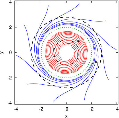
Figure 1: Phase space of the bistable Stuart-Landau oscillator for $a=1,b=2,c=2.8,\gamma=1,\beta=0.01$. Dashed lines: stable cycles; green dots: unstable cycle. Red lines: isochrons of cycle 1; blue lines: isochrons of cycle 2. Black arrows show two kicks: one moves a point on the cycle 1 to the basin of the same cycle (this kick leads to a PRC); another one moves a point on the cycle 1 to the basin of the cycle 2 (this kick leads to a PTC).

IV.2 PRC and PTC for the bistable Stuart-Landau oscillator

Now we derive the PRC and the PTC for the oscillator (2). We assume that the external action is a kick with strength $A$ in $x$-direction: $x\to x+A$. Consider a point on the cycle 1 with the phase $\varphi^{(1)}$. In the polar coordinates the point just after the kick is

$$\tilde{r}=\sqrt{(a\cos\varphi^{(1)}+A)^{2}+a^{2}\sin^{2}\varphi^{(1)}},\qquad\tilde{\theta}=\text{ATAN2}(a\sin\varphi^{(1)},a\cos\varphi^{(1)}+A)\;.$$

This point lies in the basin of cycle 1 if $\tilde{r}<b$, otherwise it belongs to the basin of cycle 2. Thus, according to expressions (4),(6), the new phases are

$$\varphi^{(1)}_{new} =\tilde{\theta}+f_{1}(\tilde{r})\qquad\text{if}\quad\tilde{r}<b\;,$$ (8)

$$\varphi^{(2)}_{new} =\tilde{\theta}+f_{2}(\tilde{r})\qquad\text{if}\quad\tilde{r}>b\;.$$ (9)

Similar expressions describe the target phase if the source point is on cycle 2:

$$\varphi^{(1)}_{new} =\bar{\theta}+f_{1}(\bar{r})\qquad\text{if}\quad\bar{r}<b\;,$$ (10)

$$\varphi^{(2)}_{new} =\bar{\theta}+f_{2}(\bar{r})\qquad\text{if}\quad\bar{r}>b\;,$$ (11)

where

$$\bar{r}=\sqrt{(c\cos\varphi^{(2)}+A)^{2}+c^{2}\sin^{2}\varphi^{(2)}},\qquad\bar{\theta}=\text{ATAN2}(c\sin\varphi^{(2)},c\cos\varphi^{(2)}+A)\;.$$

These expressions give the analytic forms of $\text{PRC}^{(1\to 1)}$ (8), of $\text{PTC}^{(1\to 2)}$ (9), of $\text{PRC}^{(2\to 2)}$ (11), and of $\text{PTC}^{(2\to 1)}$ (10).

We illustrate these curves in Figs. 2,3,4. Fig. 2 shows a case of small kick amplitudes, where there is no transition between the cycles. As a result, only PRCs exist, and there are no PTCs. For an intermediate kick amplitude, there is a possibility for a transition from cycle 2 to cycle 1, but not in the opposite direction (Fig. 3). Finally, for a large kick amplitude, all transitions are possible and all PRCs and PTCs exist (Fig. 4).

An important feature of PTCs and PRCs in the case where PTCs exist, is the singularity of these curves at the boundaries of domains of their definition. The analytic nature of these singularities is determined by terms $\sim\log|r^{2}-b^{2}|$ in expressions (5),(7). The points which are mapped to a vicinity of the basin boundary $r=b$, spend a logarithmically long time before they are attracted to stable cycles 1 or 2, and during this time interval, an extreme sensitivity of the final phase with respect to the initial one is reached. Formally, there is a phase at which both the PRC and the PTC are not defined, this is the point which is mapped exactly on the basin boundary.

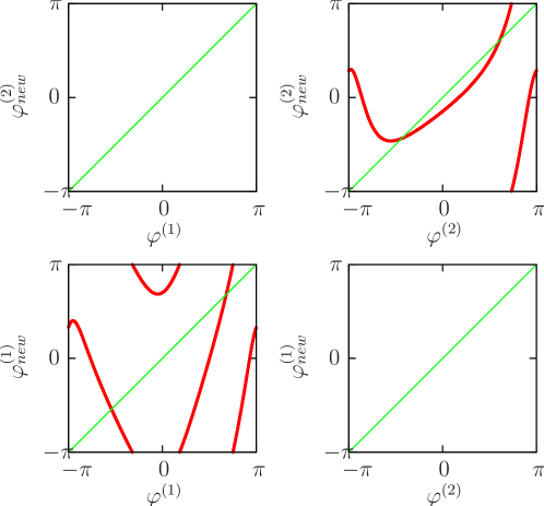
Figure 2: PRC and PTC for the same parameters as in Fig. 1 and $A=0.67$. Two diagonal panels show the PRCs $\varphi^{(1)}\to\varphi^{(1)}_{new}$ and $\varphi^{(2)}\to\varphi^{(2)}_{new}$. Two non-diagonal panels that should show PTCs ($\varphi^{(1)}\to\varphi^{(2)}_{new}$ and $\varphi^{(2)}\to\varphi^{(1)}_{new}$) are in fact empty for this small forcing (no transition from one cycle to another one); however the same plots for larger forcing in Figs. 3 and 4 do show nontrivial PTCs.

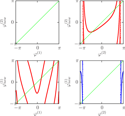
Figure 3: The same as in Fig. 2, but for $A=0.9$. For this moderate amplitude of the kicks also the PTC $\varphi^{(2)}\to\varphi^{(1)}_{new}$ exists.

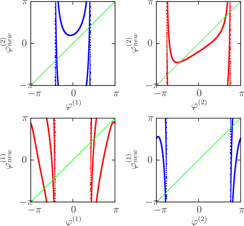
Figure 4: The same as in Fig. 2, but for $A=1.5$. For this large amplitude of the kicks all PRCs and PTCs exist.

V Periodically kicked bistable oscillator

V.1 Validity of one-dimensional approximation

In the previous section we derived the PRCs and PTCs that determine the shift of the phases under a single kick. Here we will apply them to a periodically kicked oscillator

$$\dot{x} =-y\cdot\Phi(x,y)-x\cdot R(x,y)+A\sum_{n}\delta(t-nT)\;,$$ (12)

$$\dot{y} =x\cdot\Phi(x,y)-y\cdot R(x,y)\;.$$

In the case of very large period $T$, one can assume that just prior to the next kick, the state of the system is very close to one of the stable cycles. Thus, the dynamics can be described with the one-dimensional mappings

$$\varphi^{(1)}_{n+1}=\text{PRC}^{(1\to 1)}(\varphi^{(1)}_{n}) \text{ if }r_{n}=a,\tilde{r}_{n}<b\;,$$

$$\varphi^{(2)}_{n+1}=\text{PTC}^{(1\to 2)}(\varphi^{(1)}_{n}) \text{ if }r_{n}=a,\tilde{r}_{n}>b\;,$$

$$\varphi^{(2)}_{n+1}=\text{PRC}^{(2\to 2)}(\varphi^{(2)}_{n}) \text{ if }r_{n}=c,\bar{r}_{n}>b\;,$$

$$\varphi^{(1)}_{n+1}=\text{PTC}^{(2\to 1)}(\varphi^{(2)}_{n}) \text{ if }r_{n}=c,\bar{r}_{n}<b\;.$$

This description will be not so perfect for small periods $T$, because in this case deviations from the limit cycles prior to the next kick will be significant.

To illustrate this, we first derive the exact two-dimensional mapping, with which the one-dimensional mapping based on PRCs and PTCs will be compared. Let us denote $r_{n},\varphi_{n}$ the state just prior to the $n$-th kick. Then $\theta_{n}=\varphi_{n}-f_{1,2}(r_{n})$ and $x_{n}=r_{n}\cos\theta_{n}$, $y_{n}=r_{n}\sin\theta_{n}$. Just after the kick we have

$$\hat{x}=x_{n}+A,\quad\hat{y}=y_{n},\quad\hat{r}=\sqrt{(x_{n}+A)^{2}+y_{n}^{2}},\quad\hat{\theta}=\text{ATAN2}(y_{n},x_{n}+A)\;.$$

The evolution of this point during time $T$ can be calculated using the equation for $r$:

$$\dot{r}=-\beta r(r^{2}-a^{2})(r^{2}-b^{2})(r^{2}-c^{2})\;.$$

Integration of this equation with starting point $\hat{r}$ yields

$$\frac{\ln\left|\frac{r_{n+1}^{2}-c^{2}}{\hat{r}^{2}-c^{2}}\right|}{c^{6}+a^{2}b^{2}c^{2}-c^{4}(a^{2}+b^{2})}+\frac{\ln\left|\frac{r_{n+1}^{2}-b^{2}}{\hat{r}^{2}-b^{2}}\right|}{b^{6}+a^{2}b^{2}c^{2}-b^{4}(a^{2}+c^{2})}+$$

$$+\frac{\ln\left|\frac{r_{n+1}^{2}-a^{2}}{\hat{r}^{2}-a^{2}}\right|}{a^{6}+a^{2}b^{2}c^{2}-a^{4}(b^{2}+c^{2})}-\frac{\ln\left|\frac{r_{n+1}^{2}}{\hat{r}^{2}}\right|}{a^{2}b^{2}c^{2}}=-2\beta T$$

Unfortunately, from this equation it is hardly possible to find the function $r_{n+1}(T,\hat{r})$ explicitly. This function can, however, be found numerically as a root of a function of one variable.

Depending on in which basin the point $\hat{r}$ lies, we then find $\varphi_{n+1}$ from the following expressions:

$$\varphi_{n+1}=\begin{cases}\hat{\theta}+T\Omega_{2}+f_{2}(\hat{r})&\hat{r}>b\;,\\ \hat{\theta}+T\Omega_{1}+f_{1}(\hat{r})&\hat{r}<b\;.\end{cases}$$

We now compare the results of simulations of the exact two-dimensional mapping derived, with the simulations based on the one-dimensional approximation via PRCs and PTCs. In Fig. 5 we show the case of small period $T=4$, in Fig. 6 the period is large $T=27$. In both cases we show, as functions of the kick parameter $A$, three averaged quantities. Quantity $|Z|$ characterizes the distribution of the phases, here the complex “order parameter” of the distribution of the phases is defined as $Z=\langle\exp[i\varphi_{n}]\rangle$. If the state of the system is a stable fixed point, then $|Z|=1$, otherwise $|Z|<1$ (this quantity, however, does not allow distinguishing between regular and chaotic states). Quantity $P$ describes distribution of the points between the two basins of attraction, it is calculated as $\langle\text{ind}_{n}\rangle$, where ind=1 in the basin of cycle 1 and ind=2 in the basin of cycle 2. This quantity allows distinguishing regimes belonging to one basin only, and those with switchings between the cycles 1 and 2. Finally, for the two-dimensional map we characterize deviations from the stable cycles via quantity $\Delta r=\langle(r_{n}-q_{n})^{2}\rangle^{1/2}$, where $q_{n}=a$ if $\text{ind}_{n}=1$, and $q_{n}=c$ if $\text{ind}_{n}=2$.

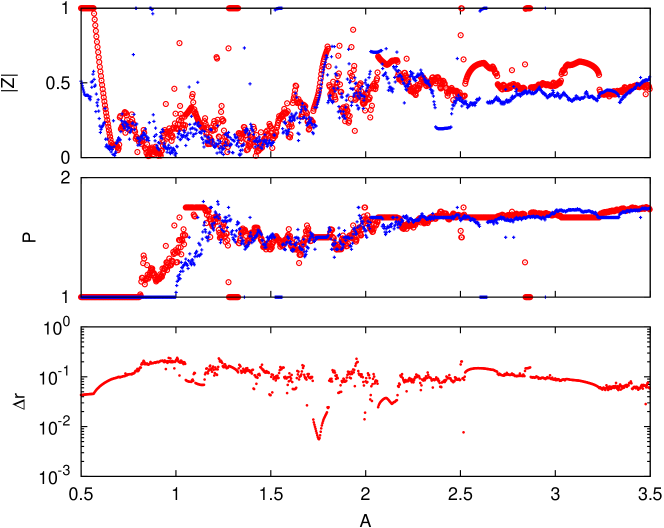
Figure 5: Comparison of the statistical properties of the dynamics (as described in the text) in the full two-dimensional system (red circles) with the one-dimensional map (blue pluses), for $T=4$. In these simulations the starting point was close to cycle 1, therefore bistability of attractors at small values of $A$ is not revealed.

Let us discuss first the quantity $\Delta r$, as it mostly directly characterizes quality of the one-dimensional approximation. One can see that for $T=27$ (Fig. 6) the typical values are $10^{-5}$, what means that here the one-dimensional map is rather close to the exact one. One can also see that the approximation is bad for special values of kick amplitude $A\approx a=1$ and $A\approx c=2.8$. The reason is that at these special values of $A$, points from the stable cycles are mapped exactly on the origin, from the vicinity of which a trajectory only slowly evolves toward the attracting cycle 1. For $T=4$ (Fig. 5) the characteristic values of $\Delta r$ are much larger, around $10^{-1}$, here one cannot expect the one-dimensional approximation to work well. This is indeed evident from the inspection of the average characteristics $|Z|$ and $P$. For $T=4$ their values in the exact solution and in the one-dimensional approximation differ significantly, while for $T=27$ they practically coincide. In Figs. 5,6 we illustrated dependence on the kick amplitude $A$ for the two selected values of time interval $T$. A more thorough study of $T$-dependence shows that the values of $\Delta r$ drastically depend on whether the regime is chaotic (like for cases $T=4$ and $T=27$ presented in Figs. 5,6), or periodic. In the latter case the values of $\Delta r$ can be as small as the accuracy of numerics $\sim 10^{-12}$. If one excludes such periodic cases, the decrease in the value of $\Delta r$ (averaged over the values of kick amplitudes in the same range as in Figs. 5,6) follows an exponential law $\langle\Delta r\rangle_{A}\sim 10^{-0.18T-0.2}$.

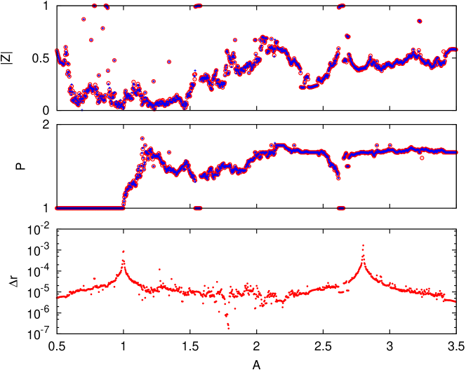
Figure 6: The same as Fig. 5, but for $T=27$.

V.2 Structure of chaos

At many parameters of forcing the bistable oscillator (12) demonstrates chaos. If the kick amplitude is small, there are no transitions from one basin to another, and the properties of chaos are similar to that of the kicked standard monostable Stuart-Landau oscillator [26]. We illustrate this regime in Fig. 7, showing the attractor near the cycle 1 for $T=4$ and $A=0.8$. One can clearly see fractal set of stripes, typical for chaotic two-dimensional sets.

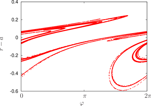
Figure 7: The strange attractor close to cycle 1 for $T=4$ and $A=0.8$.

The structure of chaos in the case where there are transitions between the basins (parameters $T=4$, $A=1.4$), Fig. 8, is more complex. Here we show a neighborhood of cycle 1 in usual coordinates, while to reveal a fine structure close to cycle 2 we plot $\log_{10}|r-c|$ vs $\varphi$. One can see that the fractal structure is somehow smeared: together with well-defined stripes there are also “scattered” points. The reason for this are extreme variations of local expansion/contraction rates at the transitions between the basins. In the one-dimensional approximation these variations are manifested by singularities of the PRCs and PTCs at the boundaries of their definition. Points of the attractor that are mapped due to a kick to a vicinity of the unstable cycle at $r=b$, are extremely scattered; to reveal a fine fractal structure of these scattered sets one needs very long trajectories.

There is also another peculiarity of the system (12): the two stable cycles for the parameters chosen have very different stability properties: the multiplier of cycle 1 is $0.42$, while for cycle 2 it is $0.072$. Therefore, close to cycle 2 the convergence is very strong, and already for moderate time intervals between the kicks $T$, distance of points to cycle 2 reaches machine zero ($\approx 10^{-14}$) for double precision calculations. One can see in Fig. 8, that already for $T=4$ a typical distance of the attractor from the cycle 2 is $\sim 10^{-8}$. For $T\approx 8$, the machine accuracy is reached, and no reliable calculations with double precision of the structure of an attractor close to cycle 2 are possible.

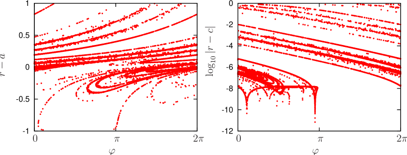
Figure 8: The strange attractor in the basin of cycle 1 (left panel) and in the basin of cycle 2 (right panel) for $T=4$ and $A=1.4$. Stripes on the right panel cross because the absolute value is used for the observable shown.

VI Conclusion

Summarizing, in this paper we have generalized the concept of phase response curves on the case of multistable periodic oscillators. The transitions from one basin to another one can be described by the phase transfer curves. We presented a solvable example, where both phase response curves and phase transfer curves can be found analytically. Furthermore, we checked how good is the phase approximation, based solely on the PRCs and PTCs, in comparison with exact solutions where the variations of the amplitudes are not neglected. While for the illustration only the solvable model of a bistable Start-Landau-type oscillator have been used, we do not see any restriction in application of the concept to other systems with different types of the phase dynamics and of the phase sensitivity (e.g., to relaxation oscillations). Furthermore, the methods of experimental determination of a PRC [11] can be straightforwardly extended to PTC determination as well.

- [1] C. C. Canavier. Phase response curve. 1(12):1332, 2006.
- [2] A. Pikovsky, M. Rosenblum, and J. Kurths. Synchronization. A Universal Concept in Nonlinear Sciences. Cambridge University Press, Cambridge, 2001.
- [3] E. M. Izhikevich. Dynamical Systems in Neuroscience. MIT Press, Cambridge, Mass., 2007.
- [4] S. Abramovich-Sivan and S. Akselrod. A single pacemaker cell model based on the phase response curve. Biological Cybernetics, 79:67–76, 1998.
- [5] M. A. St Hilaire, J. J. Gooley, S. B. S. Khalsa, R. E. Kronauer, C. A. Czeisler, and S. W. Lockley. Human phase response curve to a 1h pulse of bright white light. J. Physiol., 590(13):3035–3045, 2012.
- [6] N. Ikeda. Model of bidirectional interaction between myocardial pacemakers based on the phase response curve. Biological Cybernetics, 43(3):157–167, 1982.
- [7] N. Ikeda, S. Yoshizawa, and T. Sato. Difference equation model of ventricular parasystole as an interaction between cardiac pacemakers based on the phase response curve. Journal of Theoretical Biology, 103(3):439, 1983.
- [8] S. B. S. Khalsa, M. E. Jewett, C. Cajochen, and C. A. Czeisler. A phase response curve to single bright light pulses in human subjects. J. Physiol., 549(3):945–952, 2003.
- [9] B. Kralemann, M. Frühwirth, A. Pikovsky, M. Rosenblum, T. Kenner, J. Schaefer, and M. Moser. In vivo cardiac phase response curve elucidates human respiratory heart rate variability. Nature Communications,, 4:2418, 2013.
- [10] M. Lengyel, J. Kwag, O. Paulsen, and P. Dayan. Matching storage and recall: hippocampal spike timing-dependent plasticity and phase response curves. Nature Neuroscience, 8:1677 – 1683, 2005.
- [11] R. F. Galán, G. B. Ermentrout, and N. N. Urban. Efficient Estimation of Phase-Resetting Curves in Real Neurons and its Significance for Neural-Network Modeling. Phys. Rev. Lett., 94:158101, 2005.
- [12] T. Harada, H.-A. Tanaka, M. J. Hankins, and I. Z. Kiss. Optimal waveform for the entrainment of a weakly forced oscillator. Phys. Rev. Lett., 105:088301, 2010.
- [13] A. Zlotnik, Y. Chen, I. Z. Kiss, H.-A. Tanaka, and J.-S. Li. Optimal waveform for fast entrainment of weakly forced nonlinear oscillators. Phys. Rev. Lett., 111:024102, 2013.
- [14] A. Pikovsky. Maximizing coherence of oscillations by external locking. Phys. Rev. Lett., 115:070602, Aug 2015.
- [15] C. I. Eastman and H. J. Burgess. How to travel the world without jet lag. Sleep Med. Clin., 4(2):241–255, 2009.
- [16] C. H. Johnson. Phase Response Curves: What Can They Tell Us About Circadian Clocks? In T. Hiroshige, K. Honma, editor, Circadian clocks from cell to human : Proceedings of the Fourth Sapporo Symposium on Biological Rhythm, pages 209–249, Sapporo, 1991. Hokkaido University Press.
- [17] T. Ohara, H. Fukuda, and I. T. Tokuda. Phase Response of the Arabidopsis thaliana Circadian Clock to Light Pulses of Different Wavelengths. Journal of Biological Rhythms, 30(2):95–103, 2015.
- [18] Y.-S. Wei and H.-J. Lee. Adjustability of the circadian clock in the cockroaches: a comparative study of two closely, related species, Blattella germanica And Blattella bisignata. Chronobiology International, 18(5):767–780, 2001.
- [19] O. V. Popovych and P. A. Tass. Desynchronizing electrical and sensory coordinated reset neurostimulation. Front. Hum. Neurosci., 6:58, 2012.
- [20] J. Schwabedal, A. Pikovsky, B. Kralemann, and M. Rosenblum. Optimal phase description of chaotic oscillators. Phys. Rev. E, 85:026216, 2012.
- [21] J. T. C. Schwabedal and A. Pikovsky. Phase description of stochastic oscillations. Phys. Rev. Lett., 110:134101, 2013.
- [22] J. Guckenheimer. Isochrons and phaseless sets. J. Math. Biology, 1:259–273, 1975.
- [23] W. Z. Zeng, L. Glass, and A. Shrier. The topology of phase response curves induced by single and paired stimuli. J. Biol. Rhythms, 7:89–104, 1992.
- [24] G. P. Krishnan, M. Bazhenov, and A. Pikovsky. Multi-pulse phase resetting curve. Phys. Rev. E, 88:042902, 2013.
- [25] V. Klinshov, S. Yanchuk, A. Stephan, and V. Nekorkin. Phase response function for oscillators with strong forcing or coupling. EPL (Europhysics Letters), 118(5):50006, 2017.
- [26] G. M. Zaslavsky. The symplest case of a strange attractor. Phys. Lett. A, 69(3):145–147, 1978.