Inexact methods for symmetric stochastic eigenvalue problems

Abstract

We study two inexact methods for solutions of random eigenvalue problems in the context of spectral stochastic finite elements. In particular, given a parameter-dependent, symmetric matrix operator, the methods solve for eigenvalues and eigenvectors represented using polynomial chaos expansions. Both methods are based on the stochastic Galerkin formulation of the eigenvalue problem and they exploit its Kronecker-product structure. The first method is an inexact variant of the stochastic inverse subspace iteration [B. Sousedík, H. C. Elman, SIAM/ASA Journal on Uncertainty Quantification 4(1), pp. 163–189, 2016]. The second method is based on an inexact variant of Newton iteration. In both cases, the problems are formulated so that the associated stochastic Galerkin matrices are symmetric, and the corresponding linear problems are solved using preconditioned Krylov subspace methods with several novel hierarchical preconditioners. The accuracy of the methods is compared with that of Monte Carlo and stochastic collocation, and the effectiveness of the methods is illustrated by numerical experiments.

1 Introduction

Eigenvalue analysis is important in a number of applications, for example in modeling of vibrations of mechanical structures, neutron transport criticality computations, or stability of dynamical systems, to name a few. The behavior of the underlying mathematical models depends on proper choice of parameters entering the model through coefficients, boundary conditions or forces. However, in practice the exact values of these parameters are not known and they are treated as random processes. The uncertainty is translated by discretization into the matrix operators and subsequently into eigenvalues and eigenvectors. The standard techniques to solve this problems include Monte Carlo (MC) methods [2, 25, 31], which are robust but relatively slow, and perturbation methods [15, 17, 32, 38], which are limited to models with low variability of uncertainty.

In this study, we use spectral stochastic finite element methods (SSFEM) [7, 18, 20, 43] for the solution of symmetric eigenvalue problems. The assumption in these methods is that the parametric uncertainty is described in terms of polynomials of random variables, and they compute solutions that are also polynomials in the same random variables in the so-called generalized polynomial chaos (gPC) framework [7, 44]. There are two main approaches: stochastic collocation (SC) and stochastic Galerkin (SG) methods. The first approach is based on sampling, so the problem is translated into a set of independent deterministic systems; the second one is based on stochastic Galerkin projection and the problem is translated into one large coupled deterministic system. While the SSFEM methods have become quite popular for solving stochastic partial differential equations, the literature addressing eigenvalue problems is relatively limited. The stochastic inverse iteration in the context of the SG framework was proposed by Verhoosel et al. [37]. Meidani and Ghanem [22, 23] formulated stochastic subspace iteration using a stochastic version of the modified Gram-Schmidt algorithm. Sousedík and Elman [33] introduced stochastic inverse subspace iteration by combining the two techniques, they showed that deflation of the mean matrix can be used to compute expansions of the interior eigenvalues, and they also showed that the stochastic Rayleigh quotient alone provides a good approximation of an eigenvalue expansion; see also [3, 4, 27] for closely related methods. The authors of [23, 33] used a quadrature-based normalization of eigenvectors. Normalization based on a solution of a small nonlinear problem was proposed by Hakula et al. [12], and Hakula and Laaksonen [13] also provided an asymptotic convergence theory for the stochastic iteration. In an alternative approach, Ghanem and Ghosh [6, 9] proposed two numerical schemes—one based on Newton iteration and another based on an optimization problem (see also [8, 10]). Most recently, Benner et al. [1] formulated an inexact low-rank Newton–Krylov method, in which the stochastic Galerkin linear systems are solved using the BiCGStab method with a variant of mean-based preconditioner. In alternative approaches, Pascual and Adhikari [28] introduced several hybrid perturbation-polynomial chaos methods, and Williams [40, 41, 42] presented a method that avoids the nonlinear terms in the conventional method of stochastic eigenvalue calculation but introduces an additional independent variable.

We formulate two inexact methods for symmetric eigenvalue problems formulated in the SSFEM framework and based on the SG formulation. The first method is an inexact variant of the stochastic inverse subspace iteration from [33], in which the linear stochastic Galerkin systems are solved using the conjugate gradient method with the truncated hierarchical preconditioner [35] (see also [36]). The second method is an inexact variant of the Newton iteration from [6], in which the linear stochastic Galerkin systems are solved using preconditioned MINRES and GMRES. The methods are derived using the Kronecker-product formulation and we also comment on the so-called matricized format. The formulation of the Newton’s method is closely related to that of [1], however we consider general parametrization of stochastic coefficients, the Jacobian matrices are symmetrized, and we propose a class of hierarchical preconditioners, which can be viewed as extensions of the hierarchical preconditioners used for the first method. We also note that we have recently successfully combined an inexact Newton–Krylov method with the stochastic Galerkin framework in a different context [19, 34]. The performance of both methods is illustrated by numerical experiments, and the results are compared to that of MC and SC methods.

The paper is organized as follows. In Section 2 we introduce the stochastic eigenvalue problem, in Section 2.1 we recall the solution techniques using sampling methods (Monte Carlo and stochastic collocation), in Section 2.2 we introduce the stochastic Galerkin formulation, in Section 3 we formulate the inverse subspace iteration and in Section 4 the Newton iteration, in Section 5.1 we report the results of numerical experiments, and in Section 6 we summarize our work. In Appendices A and B we describe algorithmic details, and in Appendix C we discuss the computational cost.

2 Stochastic eigenvalue problem

Let $D$ be a bounded physical domain, and let $\left(\Omega,\mathcal{F},\mathcal{P}\right)$ be a complete probability space, that is, $\Omega$ is the a sample space with a $\sigma$-algebra$~{}\mathcal{F}$ and a probability measure $\mathcal{P}$. We assume that the randomness in the mathematical model is induced by a vector $\xi:\Omega\mapsto\Gamma\subset\mathbb{R}^{m_{\xi}}$ of independent, identically distributed random variables $\xi_{1}(\omega),\dots,\xi_{m_{\xi}}(\omega)$, where $\omega\in\Omega$. Let $\mathcal{B}(\Gamma)$ denote the Borel $\sigma$-algebra on$~{}\Gamma$ induced by $\xi$ and $\mu$ denote the induced measure. The expected value of the product of measurable functions on$~{}\Gamma$ determines a Hilbert space $T_{\Gamma}\equiv L^{2}\left(\Gamma,\mathcal{B}(\Gamma),\mu\right)$ with inner product

$$\left\langle u,v\right\rangle=\mathbb{E}\left[uv\right]=\int_{\Gamma}u(\xi)v(\xi)\,\mu(\xi)d\xi,$$ (1)

where the symbol $\mathbb{E}$ denotes the mathematical expectation.

In computations we will use a finite-dimensional subspace $T_{p}\subset T_{\Gamma}$ spanned by a set of multivariate polynomials $\left\{\psi_{\ell}(\xi)\right\}$ that are orthonormal with respect to the density function $\mu$, that is $\mathbb{E}\left[\psi_{k}\psi_{\ell}\right]=\delta_{k\ell}$, where$~{}\delta_{k\ell}$ is the Kronecker delta, and $\psi_{0}$ is constant. This will be referred to as the gPC basis [44]. The dimension of the space$~{}T_{p}$ depends on the polynomial degree. For polynomials of total degree$~{}p$, the dimension is $n_{\xi}=\binom{m_{\xi}+p}{p}$. We suppose we are given a symmetric matrix-valued random variable$~{}A(x,\xi)$ represented as

$$A(x,\xi)=\sum_{\ell=1}^{n_{a}}A_{\ell}(x)\psi_{\ell}(\xi),$$ (2)

where each$~{}A_{\ell}$ is a deterministic matrix of size $n_{x}\times n_{x}$ with size determined by the discretization of the physical domain, and $A_{1}$ is the mean value matrix, that is $A_{1}=\mathbb{E}\left[A(x,\cdot)\right]$. The representation (2) is obtained from either the Karhunen-Loève expansion or, more generally, a stochastic expansion of an underlying random process.

We are interested in a solution of the following stochastic eigenvalue problem: find a set of stochastic eigenvalues $\lambda^{s}$ and corresponding eigenvectors $u^{s}$, $s=1,\dots,n_{s}$, which almost surely (a.s.) satisfy the equation

$$A(x,\xi)u^{s}(x,\xi)=\lambda^{s}(\xi)u^{s}(x,\xi),\qquad\forall x\in D,$$ (3)

where $\lambda^{s}(\xi)\in\mathbb{R}$ and $u^{s}(\xi)\in\mathbb{R}^{n_{x}}$, along with a normalization condition

$$\left\langle{u^{s}(x,\xi)},u^{s}(x,\xi)\right\rangle_{\mathbb{R}}=1,$$ (4)

where $\left\langle\cdot,\cdot\right\rangle_{\mathbb{R}}$ denotes the inner product of two vectors.

We will search for expansions of eigenpairs$~{}{(\lambda^{s},u^{s})}$, $s=1,\dots,n_{s}$, in the form

$$\lambda^{s}(\xi)=\sum_{k=1}^{n_{\xi}}\lambda_{k}^{s}\psi_{k}(\xi),\qquad u^{s}(x,\xi)=\sum_{k=1}^{n_{\xi}}u_{k}^{s}\psi_{k}(\xi),$$ (5)

where $\lambda_{k}^{s}\in\mathbb{R}$ and $u_{k}^{s}\in\mathbb{R}^{n_{x}}$ are the coefficients corresponding to the basis $\left\{\psi_{k}\right\}$. Equivalently to (5), using the symbol $\otimes$ for the Kronecker product, we write

$$\lambda^{s}(\xi)=\Psi(\xi)^{T}\bar{\lambda}^{s},\qquad u^{s}(x,\xi)=(\Psi(\xi)^{T}\otimes I_{n_{x}})\bar{u}^{s},$$ (6)

where $\Psi(\xi)=[\psi_{1}(\xi),\ldots,\psi_{n_{\xi}}(\xi)]^{T}$, $\bar{\lambda}^{s}=[\lambda_{1}^{s},\ldots,\lambda_{n_{\xi}}^{s}]^{T}$, and $\bar{u}^{s}=[(u_{1}^{s})^{T},\ldots(u_{n_{\xi}}^{s})^{T}]^{T}$.

Remark 1.

One can in general consider different number of terms in the two expansions (5). However, since the numerical experiments in [33] and also in the present work indicate virtually no effect when the number of terms in eigenvalue expansion is larger than in the eigenvector expansion, we consider here the same number of terms in both expansions, see also Remark 2.

2.1 Sampling methods

Both Monte Carlo and stochastic collocation methods are based on sampling. The coefficients are defined by a discrete projection

$$\lambda_{k}^{s}=\left\langle\lambda^{s},\psi_{k}\right\rangle,\quad k=1,\dots,n_{\xi},\qquad u_{k}^{s}=\left\langle u^{s},\psi_{k}\right\rangle,\quad k=1,\dots,n_{\xi}.$$ (7)

The evaluations of coefficients in (7) entail solving a set of independent deterministic eigenvalue problems at a set of sample points$~{}\xi^{(q)}$, $q=1,\dots,n_{MC}$ or$~{}n_{q}$,

$$A(\xi^{(q)})u^{s}(\xi^{(q)})=\lambda^{s}\left(\xi^{(q)}\right)u^{s}\left(\xi^{(q)}\right),\qquad s=1,\dots,n_{s}.$$

In the Monte Carlo method, the sample points$~{}\xi^{(q)}$, $q=1,\dots,n_{MC},$ are generated randomly following the distribution of the random variables$~{}\xi_{i}$, $i=1,\dots,m_{\xi}$, and moments of solution are computed by ensemble averaging. In addition, the coefficients in (5) can be computed as

$$\lambda_{k}^{s}=\frac{1}{n_{MC}}\sum_{q=1}^{n_{MC}}\lambda^{s}(\xi^{(q)})\psi_{k}\left(\xi^{(q)}\right),\qquad u_{mk}^{s}=\frac{1}{n_{MC}}\sum_{q=1}^{n_{MC}}u^{s}(x_{m},\mathbb{\xi}^{(q)})\psi_{k}(\mathbb{\xi}^{(q)}),$$

where $u_{mk}^{s}$ is the $m$th element of $u_{k}^{s}$. For stochastic collocation, which is used here in the form of so-called nonintrusive stochastic Galerkin method, the sample points$~{}\xi^{(q)}$, $q=1,\dots,n_{q},$ consist of a predetermined set of collocation points, and the coefficients $\lambda_{k}^{s}$ and $u_{k}^{s}$ in expansions (5) are determined by evaluating (7) in the sense of (1) using numerical quadrature

$$\lambda_{k}^{s}=\sum_{q=1}^{n_{q}}\lambda^{s}(\mathbb{\xi}^{(q)})\psi_{k}(\mathbb{\xi}^{(q)})w^{(q)},\qquad u_{mk}^{s}=\sum_{q=1}^{n_{q}}u^{s}(x_{m},\mathbb{\xi}^{(q)})\psi_{k}(\mathbb{\xi}^{(q)})w^{(q)},$$ (8)

where $\mathbb{\xi}^{(q)}$ are the quadrature (collocation) points and $w^{(q)}$ are quadrature weights. We refer, e.g., to [18] for a discussion of quadrature rules. Details of the rule we use in our numerical experiments are discussed in Section 5.1.

2.2 Stochastic Galerkin formulation

The main contribution of this paper is the development of two inexact methods based on the stochastic Galerkin formulation of eigenvalue problem (3)–(4). The formulation entails a projection

$$\left\langle Au^{s},\psi_{k}\right\rangle =\left\langle\lambda^{s}u^{s},\psi_{k}\right\rangle, k =1,\dots,n_{\xi},\quad s=1,\dots,n_{s},$$ (9)

$$\left\langle u^{sT}u^{s},\psi_{k}\right\rangle =\delta_{k1}, k =1,\dots,n_{\xi},\quad s=1,\dots,n_{s}.$$ (10)

Let us introduce the notation

$$[H_{\ell}]_{kj}=h_{\ell,kj},\quad h_{\ell,kj}\equiv\mathbb{E}\left[\psi_{\ell}\psi_{k}\psi_{j}\right],\qquad\ell=1,\dots,n_{a},\quad j,k=1,\dots,n_{\xi}.$$ (11)

Substituting (2) and (5) into (9)–(10) yields a nonlinear system,

$$\left(\sum_{\ell=1}^{n_{a}}H_{\ell}\otimes A_{\ell}\right)\overline{u}^{s} = \left(\sum_{i=1}^{n_{\xi}}H_{i}\otimes\lambda_{i}^{s}I_{n_{x}}\right)\overline{u}^{s},\quad s=1,\dots,n_{s},$$ (12)

$$\sum_{j=1}^{n_{\xi}}\sum_{i=1}^{n_{\xi}}\left[H_{k}\circ\left\langle u_{i}^{s},u_{j}^{s}\right\rangle_{\mathbb{R}}\right]_{ij} = \delta_{k1},\qquad k=1,\dots,n_{\xi},\quad s=1,\dots,n_{s},$$ (13)

where the symbol$~{}\circ$ is the Hadamard product, see, e.g., [14, Chapter 5]. An equivalent formulation of (12)–(13) is obtained as follows. Substituting (6) into (3)–(4) and rearranging, we get

$$(\Psi^{T}\otimes A)\bar{u}^{s} = ((\bar{\lambda}^{s})^{T}\Psi\Psi^{T}\otimes I_{n_{x}})\bar{u}^{s},$$

$$\bar{u}^{s}{}^{T}(\Psi(\xi)\Psi(\xi)^{T}\otimes I_{n_{x}})\bar{u}^{s} = 1,$$

and employing Galerkin projection (9)–(10) yields the equivalent formulation

$$\mathbb{E}[\Psi\Psi^{T}\otimes A]\bar{u}^{s} = \mathbb{E}[((\bar{\lambda}^{s})^{T}\Psi)\Psi\Psi^{T}\otimes I_{n_{x}})]\bar{u}^{s},$$ (14)

$$\mathbb{E}[\Psi\otimes(\bar{u}^{s}{}^{T}(\Psi\Psi^{T}\otimes I_{n_{x}})\bar{u}^{s})] = \mathbb{E}[\Psi\otimes 1].$$ (15)

Finally, we note that the methods can be equivalently formulated in the so-called matricized format, which can also simplify the implementation. To this end, we make use of isomorphism between $\mathbb{R}^{n_{x}n_{\xi}}$ and $\mathbb{R}^{n_{x}\times n_{\xi}}$ determined by the operators vec and mat: $\bar{u}^{s}=\text{vec}(\bar{U}^{s})$, $\bar{U}^{s}=\text{mat}$($\bar{u}^{s})$, where $\bar{u}^{s}\in\mathbb{R}^{n_{x}n_{\xi}}$, $\bar{U}^{s}\in\mathbb{R}^{n_{x}\times n_{\xi}}$ and the upper/lower case notation is assumed throughout the paper, so $\bar{R}^{s}=\text{mat}$($\bar{r}^{s})$, etc. Specifically, we define the matricized coefficients of the eigenvector expansion

$$\bar{U}^{s}=\text{mat}(\bar{u}^{s})=\left[u_{1}^{s},u_{2}^{s},\ldots,u_{n_{\xi}}^{s}\right]\in\mathbb{R}^{n_{x}\times n_{\xi}},$$ (16)

where the column $k$ contains the coefficients associated with the basis function$~{}\psi_{k}$.

In the rest of the paper we explore two methods for solving the eigenvalue problem (12)–(13), resp. (14)–(15): the first is based on inverse subspace iteration (Section 3), and the second one is based on Newton iteration (Section 4).

3 Inexact stochastic inverse subspace iteration

We formulate an inexact variant of the inverse subspace iteration from [33] for the solution of (12)–(13). Stochastic inverse iteration was formulated in [37] for the case when a stochastic expansion of a single eigenvalue is sought. It was suggested in [33] that the matrix $A_{1}$ can be deflated, rather than applying a shift, to find an expansion of an interior eigenvalue, and a stochastic version of modified Gram-Schmidt process [23] can be applied if more eigenvalues are of interest. In this section, we formulate an inexact variant of the stochastic inverse subspace iteration [33, Algorithm 3.2], whereby the linear systems (19) are solved only approximately using preconditioned conjugate gradient method (PCG). The method is formulated as Algorithm 1. We now describe its components in detail, and for simplicity we drop the superscript ⁽ⁿ⁾ in the description.

Algorithm 1 Inexact stochastic inverse subspace iteration

1:Find the $n_{s}$ smallest eigenpairs of

$$A_{1}\,w^{s}=\mu^{s}\,w^{s},\qquad s=1,\dots,n_{s}.$$ (17)

2:if $\mu^{1}=\min(\mu^{s})>0$, set $\rho=0$, else shift $A_{1}=A_{1}+\rho I_{n_{x}}$, where $\rho>|\mu^{1}|$. end if

3:Initialize

$$u_{1}^{s,\left(0\right)}=w^{s},\quad u_{i}^{s,\left(0\right)}=0,\qquad s=1,\dots,n_{s},\quad i=2,\dots,n_{\xi}.$$ (18)

4:for $n=0,1,2,\dots$ do

5:     Use conjugate gradients with preconditioner from Algorithm 2 or 3 to solve

$$\left(\sum_{\ell=1}^{n_{a}}H_{\ell}\otimes A_{\ell}\right)\overline{v}^{s,(n)}=\overline{u}^{s,(n)},\quad s=1,\dots,n_{s}.$$ (19)

6:     if $n_{s}=1$ then normalize using the quadrature rule (24): $\overline{u}^{1,\left(n+1\right)}\leftarrow\overline{v}^{1,\left(n\right)}$.

7:     else orthogonalize using the stochastic modified Gram-Schmidt process:
${}\qquad\qquad\overline{u}^{s,\left(n+1\right)}\leftarrow\overline{v}^{s,\left(n\right)},\quad s=1,\dots,n_{s}$.

8:     end if

9:     Check convergence.

10:end for

11:Use the stochastic Rayleigh quotient (21) to compute the eigenvalue expansions.

12:if $\rho>0$, shift $\lambda_{1}^{s}=\lambda_{1}^{s}-\rho$ for $s=1,\dots,n_{s}$. end if

Matrix-vector product

The conjugate gradient method and computation of the stochastic Rayleigh quotient require a stochastic version of a matrix-vector product, which corresponds to evaluation of the projection

$$v_{k}^{s}=\left\langle v^{s},\psi_{k}\right\rangle=\left\langle Au^{s},\psi_{k}\right\rangle,\qquad k=1,\dots,n_{\xi}.$$

Since $(V\otimes W)\text{vec}(X)=\text{vec}(WXV^{T})$, the coefficients of the expansion are

$$\bar{v}^{s}=\mathbb{E}[\Psi\Psi^{T}\otimes A]\bar{u}^{s}=\sum_{\ell=1}^{n_{a}}({H}_{\ell}\otimes A_{\ell})\bar{u}^{s}\quad\Leftrightarrow\quad\bar{V}^{s}=\sum_{\ell=1}^{n_{a}}A_{\ell}\bar{U}^{s}H_{\ell}^{T}.$$ (20)

The use of this computation for the Rayleigh quotient is described below. We also note that Algorithm 1 can be modified to perform subspace iteration [23, Algorithm $4$] for identifying the largest eigenpairs. In this case, the solve (19) is simply replaced by a matrix-vector product (20).

Stochastic Rayleigh quotient

In the deterministic case, the Rayleigh quotient is used to compute the eigenvalue corresponding to a normalized eigenvector$~{}u$ as $\lambda=u^{T}v$, where $v=Au$. For the stochastic Galerkin method, the Rayleigh quotient defines the coefficients of a stochastic expansion of the eigenvalue defined via a projection

$$\lambda_{k}^{s}=\left\langle\lambda^{s},\psi_{k}\right\rangle=\left\langle u^{s}{}^{T}v^{s},\psi_{k}\right\rangle,\qquad k=1,\dots,n_{\xi}.$$

The coefficients of$~{}v^{s}$ are computed using (20) and the coefficients$~{}\lambda_{k}^{s}$ are

$$\lambda_{k}^{s}=\mathbb{E}\left[\left(\left(\Psi^{T}\otimes 1\right)\bar{\lambda}^{s}\right)\psi_{k}\right]=\mathbb{E}\left[\left(\bar{u}^{sT}\left(\Psi\Psi^{T}\otimes I_{n_{x}}\right)\bar{v}^{s}\right)\,\psi_{k}\right],\qquad k=1,\dots,n_{\xi},$$

which is

$$\lambda_{k}^{s}=\sum_{j=1}^{n_{\xi}}\sum_{i=1}^{n_{\xi}}\left[H_{k}\circ\left\langle u_{i}^{s},v_{j}^{s}\right\rangle_{\mathbb{R}}\right]_{ij}=\sum_{j=1}^{n_{\xi}}\sum_{i=1}^{n_{\xi}}\left[H_{k}\circ\left(\bar{U}^{sT}\bar{V}^{s}\right)\right]_{ij},\qquad k=1,\dots,n_{\xi}.$$ (21)

Remark 2.

The Rayleigh quotient (21) finds $n_{\xi}$ coefficients of the eigenvalue expansion, which is consistent with Newton iteration formulated in Section 4 and also with the literature [23, 37]. We note that it would be possible to compute the coefficients$~{}\lambda_{k}$ for $k>n_{\xi}$ as well, because the inner product $u^{T}v$ of two eigenvectors which are expanded using chaos polynomials up to degree $p$ has nonzero chaos coefficients up to degree $2p$. An alternative is to use a full representation of the Rayleigh quotient based on the projection of $u^{T}Au$. However, from our experience in the present and the previous work [33], the representation (21) is sufficient.

Normalization and the Gram-Schmidt process

Let $~{}\left\|\cdot\right\|_{2}$ denote the vector norm, induced by the inner product$~{}\left\langle\cdot,\cdot\right\rangle_{\mathbb{R}}$. That is, for a vector$~{}u$ evaluated at a point$~{}\xi$,

$$\left\|u\left(\xi\right)\right\|_{2}=\sqrt{\sum_{n=1}^{n_{x}}\left(\left[u\left(\xi\right)\right]_{n}\right)^{2}}.$$ (22)

At each step of stochastic iteration the coefficients of a given set of vectors$~{}\left\{v^{s}\right\}_{s=1}^{n_{s}}$ are transformed into an orthonormal set$~{}\left\{u^{s}\right\}_{s=1}^{n_{s}}$ such that the condition

$$\left\langle u^{s}\left(\xi\right),u^{t}\left(\xi\right)\right\rangle_{\mathbb{R}}=\delta_{st},\qquad\text{a.s}.,$$ (23)

and in particular (13), is satisfied. We adopt the same strategy as in [23, 33], whereby the coefficients of the orthonormal eigenvectors are calculated using a discrete projection and a quadrature rule. An alternative approach to normalization, based on solution of a relatively small nonlinear system was proposed by Hakula et al. [12].

Let us first consider normalization of a vector, so $n_{s}=1$. The coefficients in column$~{}k$ of$~{}\bar{U}^{1}$ corresponding to coefficients of a normalized vector are computed as

$$u_{k}^{1}=\sum_{q=1}^{n_{q}}\frac{v^{1}\left(\xi^{\left(q\right)}\right)}{\left\|v^{1}\left(\xi^{\left(q\right)}\right)\right\|_{2}}\,\psi_{k}\left(\xi^{\left(q\right)}\right)\,w^{\left(q\right)}.$$ (24)

When $n_{s}>1$, the orthonormalization (23) is performed by a combination of stochastic Galerkin projection and the modified Gram-Schmidt algorithm as proposed in [23],

$$\mathbb{E}\left[\Psi\otimes u^{s}\right]=\mathbb{E}\left[\Psi\otimes v^{s}\right]-\sum_{t=1}^{s-1}\mathbb{E}\left[\Psi\otimes\left(\frac{\left\langle v^{s},u^{t}\right\rangle_{\mathbb{R}}}{\left\langle u^{t},u^{t}\right\rangle_{\mathbb{R}}}u^{t}\right)\right],\quad s=2,\dots,n_{s},$$ (25)

Using the expansion (6) and rearranging, the coefficients in column$~{}k$ of$~{}\bar{U}^{s}$ are

$$u_{k}^{s}=v_{k}^{s}-\sum_{t=1}^{s-1}\chi_{k}^{ts},\qquad k=1,\dots,n_{\xi},\quad s=2,\dots,n_{s},$$

where

$$\chi^{ts}(\xi)=\frac{\left\langle v^{s}(\xi),u^{t}(\xi)\right\rangle_{\mathbb{R}}}{\left\langle u^{t}(\xi),u^{t}(\xi)\right\rangle_{\mathbb{R}}}u^{t}(\xi),$$

and the coefficients $\chi_{k}^{ts}$ are computed using a discrete projection as in (8),

$$\chi_{k}^{ts}=\sum_{q=1}^{n_{q}}\chi^{ts}\left(\xi^{\left(q\right)}\right)\,\psi_{k}\left(\xi^{\left(q\right)}\right)\,w^{\left(q\right)}.$$

Stopping criteria

The inexact iteration entails in each step of Algorithm 1 a solution of the stochastic Galerkin problem (19) using the preconditioned conjugate gradient method. We use the criteria proposed by Golub and Ye [11, Eq. (1)]; the criteria is satisfied when the relative residual of PCG gets smaller than a factor of the nonlinear residual from the previous step, that is

$$\frac{\|\overline{u}^{s,(n)}\!-\!\left(\sum_{\ell=1}^{n_{a}}H_{\ell}\otimes A_{\ell}\right)\!\overline{v}^{s,(n)}\|_{2}}{\|\overline{u}^{s,(n)}\|_{2}}\!<\!\tau\left\|{\left(\sum_{\ell=1}^{n_{a}}H_{\ell}\otimes A_{\ell}\!-\!\sum_{i=1}^{n_{\xi}}H_{i}\otimes\lambda_{i}^{s,(n-1)}I_{n_{x}}\right)\!\overline{u}^{s,(n-1)}}\right\|_{2},$$ (26)

where the factor $\tau=10^{-2}$. It is important to note that Algorithm 1 provides only the coefficients of expansion of the projection of residual on the gPC basis, that is

$$\widetilde{r}_{k}^{s}=\left\langle Au^{s}-\lambda^{s}u^{s},\psi_{k}\right\rangle,\qquad k=1,\dots,n_{\xi},\quad s=1,\dots,n_{s}$$ (27)

One could assess accuracy using Monte Carlo sampling of this residual by computing

$$r^{s}\left(\xi^{i}\right)=A\left(\xi^{i}\right)u^{s}\left(\xi^{i}\right)-\lambda^{s}\left(\xi^{i}\right)u^{s}\left(\xi^{i}\right),\qquad i=1,\dots,N_{MC},\quad s=1,\dots,n_{s}.$$

However, in the numerical experiments we use a much less expensive computation, which is based on using coefficients$~{}\widetilde{r}_{k}^{s}$ directly as an error indicator. In particular, we monitor the norms of the terms of $\widetilde{r}_{k}^{s}$ corresponding to expected value and variance,

$$\varepsilon_{1}^{s,\left(it\right)}=\left\|\widetilde{r}_{1}^{s,\left(n\right)}\right\|_{2},\qquad\varepsilon_{\sigma^{2}}^{s,\left(it\right)}=\left\|\sum_{k=2}^{n_{\xi}}\left(\widetilde{r}_{k}^{s,\left(n\right)}\right)^{2}\right\|_{2},\qquad s=1,\dots,n_{s}.$$ (28)

3.1 Preconditioners for the stochastic inverse iteration

We use two preconditioners for problem (19) – the mean-based preconditioner [29, 30] and the hierarchical Gauss-Seidel preconditioner [35]. Both preconditioners are formulated in the Kronecker-product format and we also comment on the matricized formulation. We assume that a preconditioner$~{}M_{1}$ for the mean matrix$~{}A_{1}$ is available.

The mean-based preconditioner (MB) is listed as Algorithm 2. Since $H_{1}=I_{n_{\xi}}$, the preconditioner entails$~{}n_{\xi}$ block diagonal solves with$~{}M_{1}$, and recalling that we can write $\bar{R}^{s}=\text{mat}(\bar{r}^{s})$, $\bar{V}^{s}=\text{mat}(\bar{v}^{s})$, its action can be equivalently obtained by solving

$$M_{1}\bar{V}^{s}=\bar{R}^{s}.$$ (29)

Algorithm 2 [29, 30] Mean-based preconditioner (MB)

The preconditioner $M_{\text{MB}}:\bar{r}^{s}\longmapsto\bar{v}^{s}$ for (19) is defined as

$$\left(H_{1}\otimes M_{1}\right)\bar{v}^{s}=\bar{r}^{s}.$$

Algorithm 3 [35, Algorithm 3] Hierarchical Gauss-Seidel preconditioner (hGS)

The preconditioner $M_{\text{hGS}}:\bar{r}^{s}\longmapsto\bar{v}^{s}$ for (19) is defined as follows.

1:Set the initial solution$~{}\bar{v}^{s}$ to zero and update in the following steps:

2:Solve

$$M_{1}v_{1}^{s}=r_{1}^{s}-\mathcal{F}_{1}v_{\left(2:n_{\xi}\right)}^{s},\qquad\text{ where }\mathcal{F}_{1}=\sum_{t\in\mathcal{I}_{t}}\left(\left[h_{t,\left(1\right)\left(2:n_{\xi}\right)}\right]\otimes A_{t}\right).$$ (30)

3:for $d=1,\ldots,p-1$ do

4:     Set $\ell=\left(n_{\ell}+1:n_{u}\right),\text{ where }n_{\ell}=\binom{m_{\xi}+d-1}{d-1}\text{ and }n_{u}=\binom{m_{\xi}+d}{d}$.

5:     Solve

$$\left(I_{n_{u}-n_{\ell}}\otimes M_{1}\right)v_{\left(\ell\right)}^{s}=r_{\left(\ell\right)}^{s}-\mathcal{E}_{d+1}v_{\left(1:n_{\ell}\right)}^{s}-\mathcal{F}_{d+1}v_{\left(n_{u}+1:n_{\xi}\right)}^{s},$$ (31)

where

$$\mathcal{E}_{d+1}=\sum_{t\in\mathcal{I}_{t}}\left(\left[h_{t,\left(\ell\right)\left(1:n_{\ell}\right)}\right]\otimes A_{t}\right),\qquad\mathcal{F}_{d+1}=\sum_{t\in\mathcal{I}_{t}}\left(\left[h_{t,\left(\ell\right)\left(n_{u}+1:n_{\xi}\right)}\right]\otimes A_{t}\right).$$

6:end for

7:Set $\ell=\left(n_{u}+1:n_{\xi}\right)$.

8:Solve

$$\left(I_{n_{\xi}-n_{u}}\otimes M_{1}\right)v_{\left(\ell\right)}^{s}=r_{\left(\ell\right)}^{s}-\mathcal{E}_{p+1}v_{\left(1:n_{u}\right)}^{s},\quad\text{ where }\mathcal{E}_{p+1}=\sum_{t\in\mathcal{I}_{t}}\left(\left[h_{t,\left(\ell\right)\left(1:n_{u}\right)}\right]\otimes A_{t}\right).$$

9:for $d=p-1,\ldots,1$ do

10:     Set $\ell=\left(n_{\ell}+1:n_{u}\right),\text{ where }n_{\ell}=\binom{m_{\xi}+d-1}{d-1}\text{ and }n_{u}=\binom{m_{\xi}+d}{d}$.

11:     Solve (31).

12:end for

13:Solve (30).

The hierarchical Gauss-Seidel preconditioner (hGS) is listed as Algorithm 3. We will denote by $~{}v_{\left(i:n\right)}^{s}$ a subvector of $\bar{v}^{s}$ containing gPC coefficients $i,i+1,\dots,n$, and, in particular,$\ \bar{v}^{s}=v_{\left(1:n_{\xi}\right)}^{s}$. There are two components of the preconditioner. The first component consists of block-diagonal solves with blocks of varying sizes, but computed just as in Algorithm 2, resp. in (29). The second component is used in the setup of the right-hand sides for the solves and consists of matrix-vector products by certain subblocks of the stochastic Galerkin matrix by vectors of corresponding sizes. To this end, we will write $\left[h_{t,(\ell)(k)}\right]$, with $(\ell)$ and $(k)$ denoting a set of (consecutive) rows and columns of matrix $H_{t}$ so that, in particular, ${H}_{t}=\left[h_{t,(1:n_{\xi})(1:n_{\xi})}\right]$. Then, the matrix-vector products can be written, cf. (20) and note the symmetry of$~{}H_{t}$, as

$$v_{(\ell)}^{s}=\sum_{t\in\mathcal{I}_{t}}(\left[h_{t,(\ell)(k)}\right]\otimes A_{t})u_{(k)}^{s}\quad\Leftrightarrow\quad V_{(\ell)}^{s}=\sum_{t\in\mathcal{I}_{t}}A_{t}U_{(k)}^{s}\left[h_{t,(k)(\ell)}\right],$$ (32)

where$~{}\mathcal{I}_{t}$ is an index set$~{}\mathcal{I}_{t}\subseteq\left\{1,\dots,n_{\xi}\right\}$ indicating that the matrix-vector products may be truncated. Possible strategies for truncation are discussed in [35]. In this study, we use $\mathcal{I}_{t}=\left\{1,\dots,n_{t}\right\}$ with $n_{t}=\binom{m_{\xi}+p_{t}}{p_{t}}$ for some $p_{t}\leq p$ and, in particular, we set $t=\{0,1,2\}$. We also note that, since the initial guess is zero in Algorithm 3, the multiplications by$~{}\mathcal{F}_{1}$ and $\mathcal{F}_{d+1}$ vanish from (30)–(31).

4 Newton iteration

Use of Newton iteration to solve (9)–(10) was proposed in [6], and most recently studied in [1]. We use a similar strategy also here and formulate a line-search Newton method as Algorithm 4. To begin, we consider the system of nonlinear equations (14)–(15) and rewrite it as

$$\begin{bmatrix}F(\bar{u}^{s},\bar{\lambda}^{s})\\ G(\bar{u}^{s})\end{bmatrix}=0,\qquad s=1,\dots,n_{s},$$ (33)

where

$$F(\bar{u}^{s},\bar{\lambda}^{s}) \equiv\mathbb{E}[\Psi\Psi^{T}\otimes A]\bar{u}^{s}-\mathbb{E}[((\bar{\lambda}^{s})^{T}\Psi)\Psi\Psi^{T}\otimes I_{n_{x}}]\bar{u}^{s},$$ (34)

$$G(\bar{u}^{s}) \equiv\mathbb{E}[\Psi\otimes\left((\bar{u}^{s}{}^{T}(\Psi\Psi^{T}\otimes I_{n_{x}})\bar{u}^{s})-1\right)].$$ (35)

The Jacobian matrix of (33) is

$$\mathcal{J}(\bar{u}^{s},\bar{\lambda}^{s})=\begin{bmatrix}\frac{\partial F}{\partial\bar{u}^{s}}&\frac{\partial F}{\partial\bar{\lambda}^{s}}\\ \frac{\partial G}{\partial\bar{u}^{s}}&0\end{bmatrix},$$ (36)

where

$$\frac{\partial F}{\partial\bar{u}^{s}}(\bar{\lambda}^{s}) =\mathbb{E}[\Psi\Psi^{T}\otimes A]-\mathbb{E}[((\bar{\lambda}^{s})^{T}\Psi)\Psi\Psi^{T}\otimes I_{n_{x}}],$$ (37)

$$\frac{\partial F}{\partial\bar{\lambda}^{s}}(\bar{u}^{s}) =-\mathbb{E}[\Psi^{T}\otimes(\Psi\Psi^{T}\otimes I_{n_{x}})\bar{u}^{s}],$$ (38)

$$\frac{\partial G}{\partial\bar{u}^{s}}(\bar{u}^{s}) =2\mathbb{E}[\Psi\otimes((\bar{u}^{s})^{T}(\Psi\Psi^{T}\otimes I_{n_{x}}))].$$ (39)

Step$~{}n$ of Newton iteration entails solving a linear system

$$\left[\begin{array}[]{cc}\frac{\partial F}{\partial\bar{u}^{s}}(\bar{\lambda}^{s,(n)})&\frac{\partial F}{\partial\bar{\lambda}^{s}}(\bar{u}^{s,(n)})\\ \frac{\partial G}{\partial\bar{u}^{s}}(\bar{u}^{s,(n)})&0\end{array}\right]\left[\begin{array}[]{c}\delta\overline{u}^{s}\\ \delta\overline{\lambda}^{s}\end{array}\right]=-\left[\begin{array}[]{c}F(\bar{u}^{s,(n)},\bar{\lambda}^{s,(n)})\\ G(\bar{u}^{s,(n)})\end{array}\right],$$ (40)

followed by an update of the solution

$$\left[\begin{array}[]{c}\overline{u}^{s,(n+1)}\\ \overline{\lambda}^{s,(n+1)}\end{array}\right]=\left[\begin{array}[]{c}\overline{u}^{s,(n)}\\ \overline{\lambda}^{s,(n)}\end{array}\right]+\left[\begin{array}[]{c}\delta\overline{u}^{s}\\ \delta\overline{\lambda}^{s}\end{array}\right].$$ (41)

The matrix$~{}\mathcal{J}(\bar{u}^{s},\bar{\lambda}^{s})$ is non-symmetric, but since $\frac{\partial F}{\partial\bar{\lambda}^{s}}(\bar{u}^{s,(n)})=\left[-\frac{1}{2}\frac{\partial G}{\partial\bar{u}^{s}}(\bar{u}^{s,(n)})\right]^{T}$, we modify linear system (40) in our implementation as

$$\left[\begin{array}[]{cc}\frac{\partial F}{\partial\overline{u}^{s}}(\bar{\lambda}^{s,(n)})&\frac{\partial F}{\partial\bar{\lambda}^{s}}(\bar{u}^{s,(n)})\\ \left[\frac{\partial F}{\partial\bar{\lambda}^{s}}(\bar{u}^{s,(n)})\right]^{T}&0\end{array}\right]\left[\begin{array}[]{c}\delta\overline{u}^{s}\\ \delta\overline{\lambda}^{s}\end{array}\right]=\left[\begin{array}[]{c}-F(\bar{u}^{s,(n)},\bar{\lambda}^{s,(n)})\\ \frac{1}{2}G(\bar{u}^{s,(n)})\end{array}\right],$$ (42)

which restores symmetry of linear systems solved in each step of Newton iteration. The symmetric Jacobian matrix in (42) will be denoted by$~{}J(\bar{u}^{s,(n)},\bar{\lambda}^{s,(n)})$. The hierarchical structure of the Jacobian matrix, which is due to the stochastic Galerkin projection, is illustrated by the left panel of Figure 1. The systems (42) are solved inexactly using a preconditioned Krylov subspace method, and the details of evaluation of the right-hand side and the matrix-vector product are given in Appendix A.

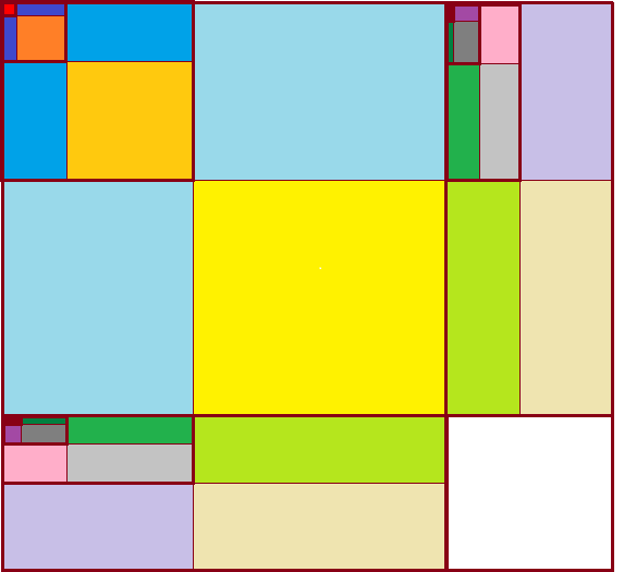
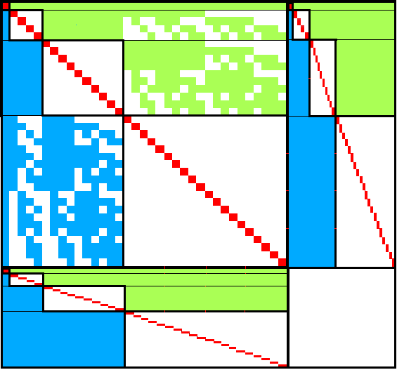
Fig. 1: Hierarchical structure of the symmetric Jacobian matrix from (42) (left) and splitting operator for the constraint hierarchical Gauss-Seidel preconditioner from Algorithm 7–8 (right).

4.1 Inexact line-search Newton method

In order to improve global convergence behavior of Newton iteration, we consider a line-search modification of the method following [26, Algorithm 11.4]. To begin, let us define the merit function as the sum of squares,

$$f(\bar{u}^{s,(n)},\bar{\lambda}^{s,(n)})=\frac{1}{2}\|r(\bar{u}^{s,(n)},\bar{\lambda}^{s,(n)})\|_{2}^{2},$$

where $r$ is the residual of (33), and denote

$$f_{n}=f(\bar{u}^{s,(n)},\bar{\lambda}^{s,(n)}),\qquad r_{n}=r(\bar{u}^{s,(n)},\bar{\lambda}^{s,(n)}),\qquad J_{n}=J(\bar{u}^{s,(n)},\bar{\lambda}^{s,(n)}).$$

As the initial approximation of the solution, we use the eigenvectors and eigenvalues of the associated mean problem given by the matrix $A_{1}$ concatenated by zeros, that is $\bar{u}^{s,(0)}=[(u_{1}^{s,(0)})^{T},0,\ldots]^{T}$ and $\bar{\lambda}^{s,(0)}=[\lambda_{1}^{s,(0)},0,\ldots]^{T}$, and the initial residual is

$$r_{0}=\begin{bmatrix}F(\bar{u}^{s,(0)},\bar{\lambda}^{s,(0)})\\ G(\bar{u}^{s,(0)})\end{bmatrix}.$$

The line-search Newton method is summarized in our setting as Algorithm 4, and the choice of parameters$~{}\rho$ and$~{}c$ in the numerical experiments is discussed in Section 5.1.

Algorithm 4 [26, Algorithm 11.4] line-search Newton method

1:Given $\rho,c\in(0,1)$, set $\alpha^{\ast}=1$.

2:Set $\bar{u}^{(0)}$ and $\bar{\lambda}^{(0)}$.

3:for $n=0,1,2,\ldots$ do

4:     $J_{n}p_{n}=-r_{n}$ (Find the Newton update $p_{n}$.)

5:     $\begin{bmatrix}\delta\bar{u}^{(n)}\\ \delta\bar{\lambda}^{(n)}\end{bmatrix}=p_{n}$

6:     $\alpha_{n}=\alpha^{\ast}$

7:     while  $f(\bar{u}^{(n)}+\alpha_{n}\delta\bar{u}^{(n)},\bar{\lambda}^{(n)}+\alpha_{n}\delta\bar{\lambda}^{(n)})>f_{n}+c\,\alpha_{n}\nabla f_{n}^{T}p_{n}$ do

8:         $\alpha_{n}\leftarrow\rho\,\alpha_{n}$

9:     end while

10:     $\bar{u}^{(n+1)}\leftarrow\bar{u}^{(n)}+\alpha_{n}\delta\bar{u}^{(n)}$

11:     $\bar{\lambda}^{(n+1)}\leftarrow\bar{\lambda}^{(n)}+\alpha_{n}\delta\bar{\lambda}^{(n)}$

12:     Check for convergence.

13:end for

The inexact iteration entails in each step a solution of the stochastic Galerkin linear system in Line 4 of Algorithm 4 given by (42) using a Krylov subspace method. In our algorithm we use the adaptive stopping criteria for the method,

$$\frac{\|r_{n}+J_{n}p_{n}\|_{2}}{\|r_{n}\|_{2}}<\tau\left\|r{{}_{n-1}}\right\|_{2},$$ (43)

where $\tau=10^{-1}$. The for-loop is terminated when the convergence check in Line 12 is satisfied; in our numerical experiments we check if $\left\|r_{n}\right\|_{2}<10^{-10}$.

4.2 Preconditioners for the Newton iteration

The Jacobian matrices in (42) are symmetric, indefinite, and so the linear systems can be ideally solved using MINRES iterative method. It is well known that a preconditioner for MINRES must be symmetric and positive definite cf., e.g., [39]. A popular choice is a block diagonal preconditioner, cf. [24],

$$\left[\begin{array}[]{cc}\widetilde{A}&0\\ 0&\widetilde{S}\end{array}\right],$$

where $\widetilde{A}\approx A$ and the Schur complement $\widetilde{S}\approx BA^{-1}B^{T}$ are obtained as approximations of the blocks in (68). Such preconditioner, based on truncation of the series in (65) and (66) to the very first term, was used in [1]. In such setup, we get

$$\widetilde{A} = I_{n_{\xi}}\otimes A_{1}-(\lambda_{1}^{s}I_{n_{\xi}}\otimes I_{n_{x}})=I_{n_{\xi}}\otimes(A_{1}-\lambda_{1}^{s}I_{n_{x}})$$

$$\approx I_{n_{\xi}}\otimes(1-\lambda_{1}^{s})(A_{1}-I_{n_{x}})$$

$$\approx I_{n_{\xi}}\otimes M_{1}^{s},$$

where the second line was used in [1]. In this study, we use the third line with

$$M_{1}^{s}=A_{1}-\epsilon_{M}\,\mu^{s}I_{n_{x}},$$ (44)

where $\mu^{s}$ is the eigenvalue of the mean problem, cf. (17). We note that it might be desirable to set the parameter $\epsilon_{M}\approx 1$, but $\epsilon_{M}\neq 1$ in order to guarantee nonsingular$~{}M_{1}^{s}$, however more details for setup and use of (44) are given in numerical experiments. Considering the first column of (66), cf. (38) and (67), we get

$$\widetilde{B}^{T}=-(I_{n_{\xi}}\otimes u_{1}^{s}),$$

and the approximation$~{}\widetilde{S}$ is

$$\widetilde{S} = (I_{n_{\xi}}\otimes u_{1}^{sT})\left[I_{n_{\xi}}\otimes(A_{1}-\lambda_{1}^{s}I_{n_{x}})\right]^{-1}(I_{n_{\xi}}\otimes u_{1}^{s})$$

$$\approx I_{n_{\xi}}\otimes\left[u_{1}^{sT}(1-\lambda_{1}^{s})^{-1}\left(A_{1}-I_{n_{x}}\right)^{-1}u_{1}^{s}\right]$$

$$\approx I_{n_{\xi}}\otimes\left[u_{1}^{sT}\left(M_{1}^{s}\right)^{-1}u_{1}^{s}\right],$$

where the second line was used in [1]. In this study, we use the third line with$~{}\left(M_{1}^{s}\right)^{-1}u_{1}^{s}$ denoting an application of$~{}M_{1}^{s}$ to$~{}u_{1}^{s}$. The ideal choice of$~{}u_{1}^{s}$ are the coefficients of the mean of eigenvector$~{}s$, and we consider two approximations here: (a) $u_{1}^{s}$ is set as the corresponding eigenvector of the mean matrix $A_{1}$, or (b) $u_{1}^{s}$ is the approximation of the gPC coefficients of the corresponding eigenvector updated after each step of Newton iteration (Algorithm 4). The preconditioners are thus either (a) fixed during Newton iteration, or (b) updated after each step. These two variants and our version of the mean-based preconditioner (NMB) for problem (42) are summarized in Algorithm 5. Clearly, if$~{}M_{1}^{s}$ is symmetric, positive definite, so is the preconditioner $M_{\text{NMB}}$, but the preconditioner loses positive definiteness if the eigenvalue of interest is not the smallest one, cf. (44), and therefore, along with MINRES, we also use GMRES and develop several preconditioners for this method.

Algorithm 5 Mean-based preconditioner for the Newton iteration (NMB)

The preconditioner $M_{\text{NMB}}:\left(\bar{r}^{(u),s},\bar{r}^{(\lambda),s}\right)\longmapsto\left(\bar{v}^{(u),s},\bar{v}^{(\lambda),s}\right)$ is defined as

$$\left[\begin{array}[]{cc}I_{n_{\xi}}\otimes M^{s}_{1}&0\\ 0&I_{n_{\xi}}\otimes\left[w^{s,(n)T}\left(M_{1}^{s}\right)^{-1}w^{s,(n)}\right]\end{array}\right]\left[\begin{array}[]{c}\bar{v}^{(u),s}\\ \bar{v}^{(\lambda),s}\end{array}\right]=\left[\begin{array}[]{c}\bar{r}^{(u),s}\\ \bar{r}^{(\lambda),s}\end{array}\right],$$ (45)

where $w^{s,(n)}$ is (a) eigenvector $w^{s}$ of $A_{1}$ corresponding to eigenvalue $\mu^{s}$, cf. (17), or (b) the first (mean) gPC coefficients $u^{s,(n)}_{1}$ of eigenvector $s$ at step $n$ of Algorithm 4.

Next, we propose a variant of so-called, constraint preconditioner, cf. [16],

$$\left[\begin{array}[]{cc}\widetilde{A}&\widetilde{B}^{T}\\ \widetilde{B}&0\end{array}\right].$$

Similarly as above, both $\widetilde{A}$ and $\widetilde{B}$ are approximations of the blocks in (68). The preconditioner is clearly indefinite (which also precludes use of MINRES). Our variant of the constraint mean-based preconditioner (cMB) is listed as Algorithm 6.

Algorithm 6 Constraint mean-based preconditioner (cMB)

The preconditioner $M_{\text{cMB}}:\left(\bar{r}^{(u),s},\bar{r}^{(\lambda),s}\right)\longmapsto\left(\bar{v}^{(u),s},\bar{v}^{(\lambda),s}\right)$ is defined as

$$\left[\begin{array}[]{cc}I_{n_{\xi}}\otimes M_{1}^{s}&-I_{n_{\xi}}\otimes w^{s,(n)}\\ -I_{n_{\xi}}\otimes w^{s,(n)T}&0\end{array}\right]\left[\begin{array}[]{c}\bar{v}^{(u),s}\\ \bar{v}^{(\lambda),s}\end{array}\right]=\left[\begin{array}[]{c}\bar{r}^{(u),s}\\ \bar{r}^{(\lambda),s}\end{array}\right],$$ (46)

where $w^{s,(n)}$ is set as in Algorithm 5.

In an analogy to Algorithm 2 and (29), the action of the preconditioners from Algorithms 5 and 6 can be equivalently obtained by solving

$$\mathcal{M}_{1}\left[\begin{array}[]{c}\bar{V}^{(u),s}\\ \bar{V}^{(\lambda),s}\end{array}\right]=\left[\begin{array}[]{c}\bar{R}^{(u),s}\\ \bar{R}^{(\lambda),s}\end{array}\right],$$ (47)

where $\mathcal{M}_{1}$ is the deterministic part the preconditioners from (45) or (46), that is

$$\mathcal{M}_{1}=\left[\begin{array}[]{cc}M_{1}^{s}&0\\ 0&w^{s,(n)T}\left(M_{1}^{s}\right)^{-1}w^{s(n)}\end{array}\right]\quad\text{or}\quad\mathcal{M}_{1}=\left[\begin{array}[]{cc}M_{1}^{s}&-w^{s(n)}\\ -w^{s,(n)T}&0\end{array}\right].$$

We also formulate a constraint version of the preconditioner from Algorithm 3, which is called a constraint hierarchical Gauss-Seidel preconditioner (chGS) and is formulated as Algorithm 7–8. There are two components of the preconditioner. The first component consists of block-diagonal solves with blocks of varying sizes computed just as in Algorithm 6, resp. (47). The second component is used in the setup of the right-hand sides for the solves and consists of matrix-vector products by certain subblocks of the stochastic Jacobian matrices by vectors of corresponding sizes. An example of matrix-vector product with a subblock of the stochastic Jacobian matrix is given in Appendix B. The preconditioner is formulated as Algorithm 7–8, and a scheme of the splitting operator is illustrated by the right panel of Figure 1. We also note that, since the initial guess is zero, the multiplications by$~{}\mathcal{F}_{1}$ and $\mathcal{F}_{d+1}$ vanish from (48)–(51).

Algorithm 7 Constraint hierarchical Gauss-Seidel preconditioner (chGS)

The preconditioner $M_{\text{chGS}}:\left(\bar{r}^{(u),s},\bar{r}^{(\lambda),s}\right)\longmapsto\left(\bar{v}^{(u),s},\bar{v}^{(\lambda),s}\right)$ is defined as follows.

1:Set the initial solution $\left(\bar{v}^{(u),s},\bar{v}^{(\lambda),s}\right)$ to zero and update in the following steps:

2:Solve

$$\mathcal{M}_{1}\left[\begin{array}[]{c}v_{1}^{(u),s}\\ v_{1}^{(\lambda),s}\end{array}\right]=\left[\begin{array}[]{c}r_{1}^{(u),s}\\ r_{1}^{(\lambda),s}\end{array}\right]-\mathcal{F}_{1}\left[\begin{array}[]{c}v_{\left(2:n_{\xi}\right)}^{(u),s}\\ v_{\left(2:n_{\xi}\right)}^{(\lambda),s}\end{array}\right],$$ (48)

where

$$\mathcal{M}_{1} = \left[\begin{array}[]{cc}M_{1}^{s}&-w^{s,(n)}\\ -w^{s,(n)T}&0\end{array}\right],\text{where }w^{s,(n)}\text{ is set as in Algorithm~{}\ref{alg:NMB},}$$

$$\mathcal{F}_{1} = \left[\begin{array}[]{cc}\sum_{t\in\mathcal{I}_{t}}\left[h_{t,\left(1\right)\left(2:n_{\xi}\right)}\right]\otimes A_{t}-\sum_{t\in\mathcal{I}_{t}}\left[h_{t,\left(1\right)\left(2:n_{\xi}\right)}\right]\otimes\lambda_{t}^{s,(n)}I_{n_{x}}&\mathcal{G}_{1}\\ \mathcal{H}_{1}&0\end{array}\right],$$

$$\mathcal{G}_{1} = \sum_{t\in\mathcal{I}_{t}}\left[h_{t,\left(1\right)\left(2:n_{\xi}\right)}\right]\otimes w_{t}^{s,(n)},$$

$$\mathcal{H}_{1} = \sum_{t\in\mathcal{I}_{t}}\left[h_{t,\left(1\right)\left(2:n_{\xi}\right)}\right]\otimes(w_{t}^{s,(n)})^{T},$$

where $w^{s,(n)}$ the eigenvector $s$ at step $n$ of Algorithm 4.

3:for $d=1,\ldots,p-1$ do

4:     Set $\ell=\left(n_{\ell}+1:n_{u}\right),\text{ where }n_{\ell}=\binom{n_{\xi}+d-1}{d-1}\text{ and }n_{u}=\binom{n_{\xi}+d}{d}$.

5:     Solve

$$\mathcal{M}_{d+1}\left[\begin{array}[]{c}v_{\left(\ell\right)}^{(u),s}\\ v_{\left(\ell\right)}^{(\lambda),s}\end{array}\right]=\left[\begin{array}[]{c}r_{\left(\ell\right)}^{(u),s}\\ r_{\left(\ell\right)}^{(\lambda),s}\end{array}\right]-\mathcal{E}_{d+1}\left[\begin{array}[]{c}v_{(1:n_{\ell})}^{(u),s}\\ v_{(1:n_{\ell})}^{(\lambda),s}\end{array}\right]-\mathcal{F}_{d+1}\left[\begin{array}[]{c}v_{(n_{u}+1:n_{\xi})}^{(u),s}\\ v_{(n_{u}+1:n_{\xi})}^{(\lambda),s}\end{array}\right],$$ (51)

where

$$\mathcal{M}_{d+1} = \left(I_{n_{u}-n_{\ell}}\!\otimes\!\left[\begin{array}[]{cc}M_{1}^{s}\!\!&\!\!-w^{s,(n)}\!\!\\ -w^{s,(n)T}\!\!&0\end{array}\right]\right),\text{where }w^{s,(n)}\text{ is set as in Algorithm~{}\ref{alg:NMB},}$$

$$\mathcal{E}_{d+1} = \left[\begin{array}[]{cc}\sum_{t\in\mathcal{I}_{t}}\left[h_{t,(\ell)\left(1:n_{\ell}\right)}\right]\otimes A_{t}-\sum_{t\in\mathcal{I}_{t}}\left[h_{t,(\ell)\left(1:n_{\ell}\right)}\right]\otimes\lambda_{t}^{s,(n)}I_{n_{x}}&\mathcal{G}_{d+1}^{\mathcal{E}}\\ \mathcal{H}_{d+1}^{\mathcal{E}}&0\end{array}\right],$$

$$\mathcal{G}_{d+1}^{\mathcal{E}} = \sum_{t\in\mathcal{I}_{t}}\left[h_{t,(\ell)\left(1:n_{\ell}\right)}\right]\otimes w_{t}^{s,(n)},$$

$$\mathcal{H}_{d+1}^{\mathcal{E}} = \sum_{t\in\mathcal{I}_{t}}\left[h_{t,(\ell)\left(1:n_{\ell}\right)}\right]\otimes(w_{t}^{s,(n)})^{T},$$

$$\mathcal{F}_{d+1} = \left[\!\begin{array}[]{cc}\sum_{t\in\mathcal{I}_{t}}\!\left[h_{t,\left(\ell\right)\left(n_{u}+1:n_{\xi}\right)}\right]\!\otimes\!A_{t}\!-\!\sum_{t\in\mathcal{I}_{t}}\!\left[h_{t,\left(\ell\right)\left(n_{u}+1:n_{\xi}\right)}\right]\!\otimes\!\lambda_{t}^{s,(n)}I_{n_{x}}&\!\mathcal{G}_{d+1}^{\mathcal{F}}\!\\ \mathcal{H}_{d+1}^{\mathcal{F}}&0\end{array}\right],$$

$$\mathcal{G}_{d+1}^{\mathcal{F}} = \sum_{t\in\mathcal{I}_{t}}\left[h_{t,\left(\ell\right)\left(n_{u}+1:n_{\xi}\right)}\right]\otimes w_{t}^{s,(n)},$$

$$\mathcal{H}_{d+1}^{\mathcal{F}} = \sum_{t\in\mathcal{I}_{t}}\left[h_{t,\left(\ell\right)\left(n_{u}+1:n_{\xi}\right)}\right]\otimes(w_{t}^{s,(n)})^{T}.$$

6:end for

Algorithm 8 Constraint hierarchical Gauss-Seidel preconditioner (chGS), continued

7:Set $\ell=\left(n_{u}+1:n_{\xi}\right)$.

8:Solve

$$\mathcal{M}_{p+1}\left[\begin{array}[]{c}v_{\left(\ell\right)}^{(u),s}\\ v_{\left(\ell\right)}^{(\lambda),s}\end{array}\right] = \left[\begin{array}[]{c}r_{\left(\ell\right)}^{(u),s}\\ r_{\left(\ell\right)}^{(\lambda),s}\end{array}\right]-\mathcal{E}_{p+1}\left[\begin{array}[]{c}v_{\left(1:n_{u}\right)}^{(u),s}\\ v_{\left(1:n_{u}\right)}^{(\lambda),s}\end{array}\right],$$

where

$$\mathcal{M}_{p+1} = \left(I_{n_{\xi}-n_{u}}\!\otimes\!\!\left[\begin{array}[]{cc}\!M_{1}^{s}\!&\!\!-w^{s,(n)}\!\!\\ \!-w^{s,(n)T}\!&0\!\end{array}\right]\right),\text{where }w^{s,(n)}\text{ is set as in Algorithm~{}\ref{alg:NMB},}$$

$$\mathcal{E}_{p+1} = \left[\begin{array}[]{cc}\sum_{t\in\mathcal{I}_{t}}\left[h_{t,(\ell)\left(1:n_{u}\right)}\right]\otimes A_{t}-\sum_{t\in\mathcal{I}_{t}}\left[h_{t,(\ell)\left(1:n_{u}\right)}\right]\otimes\lambda_{t}^{s,(n)}I_{n_{x}}&\mathcal{G}_{p+1}^{\mathcal{E}}\\ \mathcal{H}_{p+1}^{\mathcal{E}}&0\end{array}\right],$$

$$\mathcal{G}_{p+1}^{\mathcal{E}} = \sum_{t\in\mathcal{I}_{t}}\left[h_{t,(\ell)\left(1:n_{u}\right)}\right]\otimes w_{t}^{s,(n)},$$

$$\mathcal{H}_{p+1}^{\mathcal{E}} = \sum_{t\in\mathcal{I}_{t}}\left[h_{t,(\ell)\left(1:n_{u}\right)}\right]\otimes(w_{t}^{s,(n)})^{T}.$$

9:for $d=p-1,\ldots,1$ do

10:     Set $\ell=\left(n_{\ell}+1:n_{u}\right),\text{ where }n_{\ell}=\binom{n_{\xi}+d-1}{d-1}\text{ and }n_{u}=\binom{n_{\xi}+d}{d}$.

11:     Solve (51).

12:end for

13:Solve (48).

5 Numerical experiments

We implemented the methods in Matlab, and in this section we present the results of numerical experiments in which the proposed inexact solvers are applied to two benchmark problems: a diffusion problem with stochastic coefficient and stiffness of Mindlin plate with stochastic Young’s modulus.

5.1 Stochastic diffusion problem with lognormal coefficient

For the first benchmark problem we consider the elliptic equation with stochastic coefficient and deterministic Dirichlet boundary condition

$$-\nabla\cdot\left(a(x,\xi)\nabla u(x,\xi)\right) = \lambda(\xi)u(x,\xi)\quad\text{in }D\times\Gamma,$$

$$u(x,\xi) = 0\qquad\qquad\quad\;\text{on }\partial D\times\Gamma,$$

where $D$ is a two-dimensional physical domain. The uncertainty in the model is introduced by the stochastic expansion of the diffusion coefficient, considered as

$$a(x,\xi)=\sum_{\ell=1}^{n_{a}}a_{\ell}(x)\psi_{\ell}(\xi),$$ (58)

to be a truncated lognormal process transformed from the underlying Gaussian process [5]. That it, $\psi_{\ell}(\xi)$, $\ell=1,\dots,n_{a}$, is a set of Hermite polynomials and, denoting the coefficients of the Karhunen-Loève expansion of the Gaussian process by$~{}g_{j}(x)$ and $\eta_{j}=\xi_{j}-g_{j}$, $j=1,\dots,m_{\xi}$, the coefficients in expansion (58) are computed as

$$a_{\ell}(x)=\frac{\mathbb{E}\left[\psi_{\ell}(\eta)\right]}{\mathbb{E}\left[\psi_{\ell}^{2}(\eta)\right]}\exp\left[g_{0}+\frac{1}{2}\sum_{j=1}^{m_{\xi}}\left(g_{j}(x)\right)^{2}\right].$$

The covariance function of the Gaussian field, for points $X_{1}=(x_{1},y_{1})$ and $X_{2}=(x_{2},y_{2})$ in$~{}D$, was chosen to be

$$C\left(X_{1},X_{2}\right)=\sigma_{g}^{2}\exp\left(-\frac{\left|x_{2}-x_{1}\right|}{L_{x}}-\frac{\left|y_{2}-y_{1}\right|}{L_{y}}\right),$$ (59)

where$~{}L_{x}$ and $L_{y}$ are the correlation lengths of the random variables $\xi_{i}$, $i=1,\dots,m_{\xi}$, in the $x$ and $y$ directions, respectively, and $\sigma_{g}$ is the standard deviation of the Gaussian random field. According to [21], in order to guarantee a complete representation of the lognormal process by (58), the degree of polynomial expansion of $a(x,\xi)$ should be twice the degree of the expansion of the solution. We follow the same strategy here. Therefore, the values of $n_{\xi}$ and $n_{a}$ are, cf., e.g. [7, p. 87] or [43, Section 5.2], $n_{\xi}\!=\!\frac{\left(m_{\xi}+p\right)!}{m_{\xi}!p!}$, $n_{a}\!=\!\frac{\left(m_{\xi}+2p\right)!}{m_{\xi}!\left(2p\right)!}$. In the numerical experiments, the lognormal diffusion coefficient (58) is parameterized using $m_{\xi}=3$ random variables. The correlation length is $L_{\text{corr}}=2$, and the coefficient of variation $CoV$ of the lognormal process is set either to $0.1$ ($10\%)$ or $0.25$ ($25\%)$, where $CoV=\sigma/a_{1}$, the ratio of the standard deviation $\sigma$ and the mean of the diffusion coefficient$~{}a_{1}$. For the gPC expansion of eigenvalues/eigenvectors (5), the maximal degree of gPC expansion is $p=3$, so then $n_{\xi}=20$ and $n_{a}=84$.

Finite element discretization leads to a generalized eigenvalue problem

$$K(\xi)u=\lambda Mu,$$ (60)

where $K(\xi)=\sum_{\ell=1}^{n_{a}}K_{\ell}\psi_{\ell}(\xi)$ is the stochastic expansion of the stiffness matrix, and the mass matrix$~{}M$ is deterministic. Using Cholesky factorization $M=LL^{T}$, the generalized eigenvalue problem (60) can be transformed into the standard form

$$A(\xi)w=\lambda w,$$ (61)

where $u=L^{-T}w$ and the expansion of $A$ corresponding to (2) is

$$A=\sum_{\ell=1}^{n_{a}}A_{\ell}\psi_{\ell}(\xi)=\sum_{\ell=1}^{n_{a}}\left[L^{-1}K_{\ell}L^{-T}\right]\psi_{\ell}(\xi).$$ (62)

We consider the physical domain $D=[-1,1]^{2},$ discretized using a structured grid using $256$ bilinear finite elements, that is with $225$ nodes interior to$~{}D$, which determines the size of matrices$~{}A_{\ell}$ in (62). The$~{}25$ smallest eigenvalues of the mean matrix $A_{1}$ are displayed in Figure 2. For the quadrature rule, in Section 2.1, we use Smolyak sparse grid with Gauss-Hermite quadrature and grid level $4$, and $10^{4}$ samples for the Monte Carlo method. With these settings, the size of $h_{\ell,kj}$ in (11) was $84\times 20\times 20$ with $806$ nonzeros, and there were $69$ points on the sparse grid.

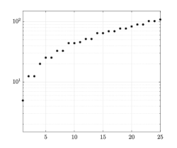
Fig. 2: The smallest 25 eigenvalues of the mean matrix $A_{1}$.

Inexact stochastic inverse subspace iteration

First, we examine the performance of the inexact stochastic inverse subspace iteration (SISI) from Algorithm 1 for computing the five smallest eigenvalues and corresponding eigenvectors of problem (61). Linear systems (19) are solved using the PCG method with the mean-based preconditioner (Algorithm 2) and the hierarchical Gauss-Seidel preconditioner (Algorithm 3). We ran the SISI algorithm with a fixed number of steps set to $20$. Figure 3 illustrates convergence history in terms of the two error indicators$~{}\epsilon_{1}$ and$~{}\epsilon_{\sigma^{2}}$ from (28) with $CoV=10\%$ (left panels) and $25\%$ (right panels). The plots were generated using the hGS preconditioner with $p_{t}=2$ ($\mathcal{I}_{t}=\{1,\ldots,10\}$), but convergence with other preconditioners was virtually identical.

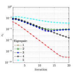
(a)

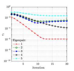
(b)

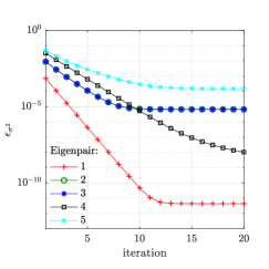
(c)

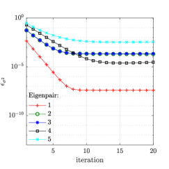
(d)

Fig. 3: Convergence history of the inexact stochastic inverse subspace iteration in terms of indicators $\epsilon_{1}$ (top) and $\epsilon_{\sigma^{2}}$ (bottom) defined by (28) with $CoV=10\%$ (left) and $25\%$ (right).

Next, we examine performance of PCG with the two preconditioners used to solve linear systems (19) with zero initial guess and stopping criterion (26). We computed the five smallest eigenvalues using 20 steps of the inexact SISI method. Table 1 shows the number of the PCG iterations required by the inexact solves, averaged over the 20 steps of the inexact SISI method for the model eigenvalue problem with $CoV=10\%$ and$~{}25\%$. Specifically, we compare the mean-based preconditioner from Algorithm 2 and the hGS preconditioner from Algorithm 3 with varying level of truncation of the matrix-vector multiplications ($p_{t}=\{0,1,2\}$ and $p_{t}=3$, i.e., no truncation). In both preconditioners we used Cholesky factorization of $A_{1}$ for the solves with$~{}M_{1}$. We note that with $p_{t}=0$ the hGS preconditioner reduces to the mean-based preconditioner. In both cases $CoV=10\%$ and $25\%$ the hGS preconditioner outperforms the mean-based preconditioner in terms of the number of PCG iterations for each of the five eigenpairs. Table 1 also shows that solving the eigenvalue problem with higher $CoV$ leads to only a slight increase in the number of iterations.

Table 1: Average number of PCG iterations for computing the five smallest eigenvalues and corresponding eigenvectors of the diffusion problem with $CoV=10\%$ (left) and $25\%$ (right) using inexact stochastic inverse subspace iteration (Algorithm 1).

	$CoV=10\%$					$CoV=25\%$
Preconditioner	1st	2nd	3rd	4th	5th	1st	2nd	3rd	4th	5th
MB	6.45	3.90	3.90	4.60	3.75	8.60	5.55	5.55	6.05	4.75
hGS ($p_{t}=1$)	3.10	1.95	1.95	2.25	1.95	3.65	2.75	2.75	2.65	2.00
hGS ($p_{t}=2$)	2.35	1.70	1.70	1.65	1.00	2.60	1.90	1.90	1.85	1.75
hGS (no trunc.)	2.15	1.00	1.00	1.45	1.00	2.60	1.80	1.80	1.75	1.65

Newton iteration

Next, we examine the inexact line-search Newton method from Algorithm 4 for computing the five smallest eigenvalues and corresponding eigenvectors of problem (61). For the line-search method, we set $\rho=0.9$ for the backtracking and limit the maximum number of backtracks to$~{}25$, and $c=0.05$. The initial guess for the nonlinear iteration is set using the (five smallest) eigenvalues and corresponding eigenvectors of the eigenvalue problem associated with the mean matrix $A_{1}$ as discussed in Section 4.1. The nonlinear iteration terminates when the norm of the residual $\|r_{n}\|_{2}<10^{-10}$. The linear systems in Line 4 in Algorithm 4 are solved using either MINRES or GMRES with the mean-based preconditioner (Algorithm 5), constraint mean-based preconditioner (Algorithm 6) and the contraint hierarchical Gauss-Seidel preconditioner (Algorithm 7–8). Figure 4 illustrates convergence history of the inexact line-search Newton method in terms of norm of the residual$~{}\|r_{n}\|_{2}$ with $CoV=10\%$ (left panel) and$~{}25\%$ (right panel). The plots were generated using GMRES with the chGS preconditioner (Algorithm 7–8) with $p_{t}=2$ ($\mathcal{I}_{t}=\{1,\ldots,10\}$), but convergence with other preconditioners was virtually identical.

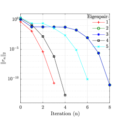
(a)

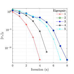
(b)

Fig. 4: Convergence history in terms of the nonlinear residual $\|r_{n}\|_{2}$ of the inexact line-search Newton method with $CoV=10\%$ (left) and $25\%$ (right).

Table 2: Average number of MINRES/GMRES iterations for computing the five smallest eigenvalues and corresponding eigenvectors of the diffusion problem with $CoV=10\%$ (left) and $25\%$ (right) using inexact line-search Newton method (Algorithm 4) with the stopping criteria $\|r_{n}\|_{2}<10^{-10}$.

	$CoV=10\%$					$CoV=25\%$
Preconditioner	1st	2nd	3rd	4th	5th	1st	2nd	3rd	4th	5th
NMB (MINRES)	11.5	59.3	60.2	23.3	217.6	13.3	110.0	109.4	49.3	142.9
NMB (fixed)	11.3	71.5	59.9	29.6	120.5	15.2	79.3	79.5	43.8	101.1
NMB (updated)	13.3	28.9	27.8	16.2	43.0	19.0	68.9	64.5	87.3	122.9
cMB (fixed)	7.0	37.9	39.5	8.8	28.1	13.3	56.6	56.6	14.6	32.4
cMB (updated)	4.3	24.7	25.4	5.3	28.0	7.8	33.4	33.1	8.6	15.6
chGS($p_{t}=1$)	2.3	17.9	17.1	2.8	15.4	3.3	18.3	18.1	2.8	18.9
chGS($p_{t}=2$)	2.0	12.4	12.5	2.0	8.5	3.3	18.9	19.4	2.4	10.3
chGS(full)	2.0	13.8	13.5	2.0	12.3	3.3	15.1	15.1	2.8	14.4

Next, we compare performance of MINRES and GMRES with the preconditioners from Algorithms 5–8 used to solve linear systems at Line 4 in Algorithm 4 with zero initial guess and the stopping criterion (43). Table 2 shows the numbers of MINRES or GMRES iterations required by the inexact solves, averaged over the number of the nonlinear steps. Specifically, we compare the mean-based preconditioner (NMB) from Algorithm 5, contraint mean-based preconditioner (cMB) from Algorithm 6 and the constraint hierarchical Gauss-Seidel preconditioner (chGS) from Algorithm 7–8. For all preconditioners, we need to select the vector$~{}w^{s,(n)}$ as discussed in Algorithm 5. Choice (a) is referred to as fixed because the vector$~{}w^{s,(n)}$ is the corresponding eigenvector of the mean matrix $A_{1}$, and choice (b) is referred to as updated because the vector is updated after each step of Newton iteration. Only the variant (b) was used for the chGS preconditioner. We also need to specify (the solves with) the matrix $M_{1}^{s}$, in particular the choice of$~{}\epsilon_{M}$ in (44). We report values of$~{}\epsilon_{M}$ that, in our experience, worked best. For (both fixed) NMB and cMB, we set $\epsilon_{M}=0.95$. For (updated) cMB and chGS, we set $\epsilon_{M}=1$ and use the SVD decomposition as $\mathcal{M}_{1}=\sum_{i=1}^{\text{rank}(\mathcal{M}_{1})}d_{i}y_{i}z_{i}^{T}$ to solve linear systems in (47). If$~{}\mathcal{M}_{1}$ appears to be numerically singular, the action of the inverse of$~{}\mathcal{M}_{1}$ is replaced by a pseudoinverse $\sum_{i=1}^{\text{rank}(\mathcal{M}_{1})}d_{i}^{-1}z_{i}y_{i}^{T}$. We note that with $p_{t}=0$ the chGS preconditioner reduces to the (updated) cMB preconditioner. With all preconditioners the convergence was faster for simple eigenvalues, and the iteration counts increased in the course of Newton iteration. In both cases with $CoV=10\%$ and $25\%$ the constraint preconditioners outperform the mean-based preconditioners, and updating the vector$~{}w^{s,(n)}$ improves the convergence. The lowest iteration counts were obtained with the chGS preconditioner, in particular with $p_{t}=2$ and full, and we note that the computational cost with $p_{t}=2$ is lower due to the truncation of the matrix-vector products. For these two preconditioners, Tables 2 and 3 show that solving the eigenvalue problem with higher $CoV$ leads to only a slight increase in the number of iterations, and for simple eigenvalues the average iteration counts are only slightly larger than those of SISI.

Table 3: The number of GMRES iterations for computing the five smallest eigenvalues and corresponding eigenvectors of the diffusion problem with $CoV=10\%$ (left) and $25\%$ (right) using inexact line-search Newton method (Algorithm 4) with preconditioners cMB (top) and chGS($p_{t}=2$) (bottom), and with the stopping criteria $\|r_{n}\|_{2}<10^{-10}$.

	$CoV=10\%$					$CoV=25\%$
	1st	2nd	3rd	4th	5th	1st	2nd	3rd	4th	5th
Nonlinear step	cMB (updated)
1	2	2	2	1	1	2	2	2	1	1
2	4	8	8	3	35	5	8	8	3	3
3	7	10	10	6	35	9	11	11	6	10
4		13	14	11	21	15	18	17	12	12
5		23	26		17		34	34	21	16
6		45	46		23		75	74		22
7		72	72		41		86	86		45
8					51
Nonlinear step	chGS($p_{t}=2$)
1	1	1	1	1	1	1	1	1	1	1
2	2	5	5	1	5	2	6	6	1	2
3	3	6	6	2	5	4	4	4	2	5
4		6	6	4	8	6	10	10	3	7
5		7	7		10		12	12	5	11
6		12	12		22		18	22		14
7		21	21				45	45		32
8		41	42				55	55

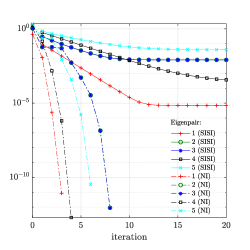
(a)

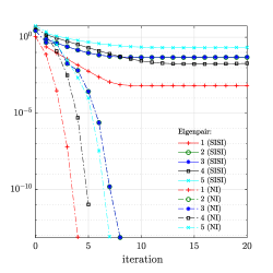
(b)

Fig. 5: Comparison of convergence of the inexact stochastic inverse subspace iteration (SISI) in terms of residual indicator $\|\bar{\widetilde{r}}^{s,\left(n\right)}\|_{2}$ and the inexact line-search Newton method (NI) in terms of $\|F(\bar{u}^{s,(n)},\bar{\lambda}^{s,(n)})\|_{2}$ with $CoV=10\%$ (left) and $25\%$ (right).

Table 4: The first $10$ coefficients of the gPC expansion of the smallest eigenvalue of the diffusion problem with $CoV=10\%$ (left) and $25\%$ (right) using stochastic collocation (SC), inexact stochastic inverse subspace iteration (SISI), and inexact line-search Newton method (NI) with the stopping criteria $\|r_{n}\|_{2}<10^{-10}$. Here $d$ is the polynomial degree and $k$ is the index of basis function in expansion (5).

		$CoV=10\%$			$CoV=25\%$
$d$	$k$	SC	SISI	NI	SC	SISI	NI
0	1	4.9431E+00	4.9431E+00	4.9431E+00	4.9052E+00	4.9052E+00	4.9052E+00
1	2	3.6197E-01	3.6197E-01	3.6197E-01	8.8127E-01	8.8127E-01	8.8127E-01
	3	1.4477E-13	-1.6489E-14	-7.9829E-16	2.0162E-13	-1.5964E-14	-7.3784E-16
	4	-6.6436E-13	-1.7135E-14	-1.3429E-15	9.9476E-14	-1.8588E-14	-1.4099E-15
2	5	1.8642E-02	1.8642E-02	1.8642E-02	1.1205E-01	1.1201E-01	1.1204E-01
	6	-5.4534E-13	-9.5178E-17	-7.4261E-17	-7.1498E-14	-2.9421E-15	-1.6150E-16
	7	-3.0909E-13	-1.1628E-15	-9.5249E-17	-9.4147E-14	-2.4433E-15	-3.7169E-16
	8	-1.5442E-03	-1.5442E-03	-1.5442E-03	-9.1479E-03	-9.1520E-03	-9.1493E-03
	9	-9.7700E-15	-1.1200E-15	1.3125E-18	-8.4643E-13	7.4442E-16	-1.2278E-17
	10	-1.5442E-03	-1.5442E-03	-1.5442E-03	-9.1479E-03	-9.1520E-03	-9.1493E-03

A comparison of the inexact SISI and the inexact Newton iteration (NI) is provided by Figure 5, which shows the $2$-norms of the residual indicator $\bar{\widetilde{r}}^{s,\left(n\right)}=[\widetilde{r}_{1}^{s,(n)T},\dots,\widetilde{r}_{n_{\xi}}^{s,(n)T}]^{T}$ from (27) and the part of the residual in the Newton method given by$~{}F(\bar{u}^{s,(n)},\bar{\lambda}^{s,(n)})$, cf. (33). These quantities correspond to the residual of eq. (9), through eq. (12) and equivalent eq. (14). It can be seen that it takes approximately the same number of steps for the NI to converge and for the SISI residuals to become flat in case of repeated eigenvalues, but more steps of SISI are needed for simple eigenvalues. With respect to the average number of Krylov iterations per a step of SISI and NI, the computational cost of the two methods is comparable for simple eigenvalues, but SISI is significantly more efficient for repeated eigenvalues. On the other hand, NI outperforms SISI in terms of accuracy of the solution residual, which is quite natural since NI is formulated as a minimization algorithm unlike SISI.

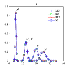
(a)

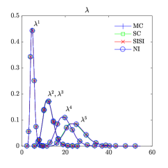
(b)

Fig. 6: Pdf estimates of the five smallest eigenvalues with $CoV=10\%$ (left) and $25\%$ (right).

We also compare the gPC coefficients of eigenvalue expansions computed using the three different methods: the stochastic collocation method, the inexact SISI method, and the inexact line-search Newton method. In Table 4, we tabulate the first ten coefficients of the gPC expansion of the smallest eigenvalues computed using the three methods. A good agreement of coefficients can be seen, in particular for coefficients with values much larger than zero, specifically with indices $k=1,2,5,8$ and$~{}10$. Figure 6 plots the probability density function (pdf) estimates of the five smallest eigenvalues obtained directly by Monte Carlo and the three methods, for which the estimates were obtained using Matlab function ksdensity used for sampled gPC expansions. It can be seen that the pdf estimates overlap in all cases.

Table 5: Average number of PCG iterations for computing the five smallest eigenvalues and corresponding eigenvectors of the diffusion problem with $CoV=10\%$ (left) and $25\%$ (right) using exact and inexact stochastic inverse subspace iteration (Algorithm 1).

		$CoV=10\%$					$CoV=25\%$
		1st	2nd	3rd	4th	5th	1st	2nd	3rd	4th	5th
MB	Inexact	6.45	3.90	3.90	4.60	3.75	8.60	5.55	5.55	6.05	4.75
	Exact	11.00	10.95	10.95	10.85	10.00	17.00	16.90	16.90	16.90	16.90
hGS	Inexact	2.35	1.70	1.70	1.65	1.00	2.60	1.90	1.90	1.85	1.75
$\!\!(p_{t}\!\!=\!\!2)\!\!$	Exact	3.00	3.00	3.00	3.00	3.00	5.00	5.00	5.00	4.00	4.00

Table 6: The number of GMRES iterations for computing the first and the fourth smallest eigenvalues and corresponding eigenvectors of the diffusion problem with $CoV=10\%$ (left) and $25\%$ (right) using exact and inexact line-search Newton method (Algorithm 4) with preconditioners cMB (top) and chGS($p_{t}=2$) (bottom), and with the stopping criteria $\|r_{n}\|_{2}<10^{-10}$.

	$CoV=10\%$				$CoV=25\%$
	Inexact		Exact		Inexact		Exact
	1st	4th	1st	4th	1st	4th	1st	4th
Nonlinear step	cMB (updated)
1	2	1	13	16	2	1	22	39
2	4	3	13	15	5	3	22	27
3	7	6	14	16	9	6	22	27
4		11		16	15	12	22	27
5						21		27
Nonlinear step	chGS($p_{t}=2$)
1	1	1	5	7	1	1	7	16
2	2	1	5	7	2	1	8	15
3	3	2	6	7	4	2	8	11
4		4		7	6	3	8	11
5						5		10
6								10

Inexact vs. exact solves

We present numerical experiments that show the effectiveness of the inexact solvers by comparing them with the exact solvers, for which we fix the stopping tolerance of the PCG and GMRES methods to $10^{-12}$. For the inexact methods we use the adaptive stopping tolerance given for SISI by (26) and for the NI by (43). A comparison of the inexact and exact solves in terms of the PCG iteration counts for computing the smallest five eigenvalues of the diffusion problem is shown in Table 5, and a comparison in terms of the GMRES iterations counts for computing the first and the fourth smallest eigenvalues of the diffusion problem is shown in Table 6. In both cases, for given $CoV$ and the choice of the preconditioner, we observe that the exact methods require more Krylov subspace iterations. It can be seen from Table 6 that virtually the same number of GMRES iterations is required in each nonlinear step of NI since the stopping tolerance of the exact solves is not adjusted to the nonlinear residual.

Effect of increasing the stochastic dimension

Table 7 shows the PCG iteration counts required to compute the smallest five eigenvalues of the diffusion problem for varying number of random variables $m_{\xi}=\{3,5,7\}$ with $CoV=10\%$ and $25\%$, and Table 8 shows the GMRES iteration counts for computing the first and fourth smallest eigenvalues for the same problem and setup. While in both cases we see a relatively small increase in iteration counts for larger $CoV$, increasing the stochastic dimension by setting larger $m_{\xi}$ appears to have no effect on the iteration counts.

Table 7: Average number of PCG iterations for computing the five smallest eigenvalues and corresponding eigenvectors of the diffusion problem with $CoV=10\%$ (left) and $25\%$ (right) for varying $m_{\xi}=\{3,5,7\}$ using inexact stochastic inverse subspace iteration (Algorithm 1).

		$CoV=10\%$					$CoV=25\%$
$m_{\xi}$	Preconditioner	1st	2nd	3rd	4th	5th	1st	2nd	3rd	4th	5th
3	MB	6.45	3.90	3.90	4.60	3.75	8.60	5.55	5.55	6.05	4.75
	hGS ($p_{t}=2$)	2.35	1.70	1.70	1.65	1.00	2.60	1.90	1.90	1.85	1.75
5	MB	6.50	3.90	3.90	4.50	3.85	8.00	4.85	4.85	6.50	4.70
	hGS ($p_{t}=2$)	2.35	1.00	1.00	1.70	1.00	2.60	1.95	1.95	1.90	1.85
7	MB	6.40	3.95	3.95	4.55	3.85	8.00	4.85	4.85	6.50	4.70
	hGS ($p_{t}=2$)	2.35	1.00	1.00	1.70	1.00	2.60	1.95	1.95	1.90	1.85

Table 8: The number of GMRES iterations for computing the first and the fourth smallest eigenvalues and corresponding eigenvectors of the diffusion problem with $CoV=10\%$ (left) and $25\%$ (right) for varying $m_{\xi}$ using inexact line-search Newton method (Algorithm 4) with preconditioners cMB (top) and chGS($p_{t}=2$) (bottom), and with the stopping criteria $\|r_{n}\|_{2}<10^{-10}$.

	$CoV=10\%$						$CoV=25\%$
$m_{\xi}$	3		5		7		3		5		7
	1st	4th	1st	4th	1st	4th	1st	4th	1st	4th	1st	4th
Nonlinear step	cMB (updated)
1	2	1	2	1	2	1	2	1	2	1	2	1
2	4	3	4	3	4	3	5	3	5	3	4	3
3	7	6	7	6	7	6	9	6	9	6	8	6
4		11		11		11	15	12	15	12	16	12
5								21		21		21
Nonlinear step	chGS($p_{t}=2$)
1	1	1	1	1	1	1	1	1	1	1	1	1
2	2	1	2	1	2	1	2	1	2	1	2	1
3	3	2	3	2	3	2	4	2	3	2	4	2
4		4		4		4	6	3	5	3	5	3
5								5		5		5

5.2 Stiffness of Mindlin plate with uniformly distributed Young’s modulus

As the second example, we study eigenvalues of the stiffness of Mindlin plate with Young’s modulus given by the stochastic expansion

$$E(x,\xi)=E_{1}+\sum_{\ell=2}^{m_{\xi}+1}E_{\ell}\xi_{\ell-1},$$ (63)

where $E_{\ell+1}=\sqrt{\lambda_{\ell}}v_{\ell}(x)$ with $\{\left(\lambda_{\ell},v_{\ell}\right)\}_{\ell=1}^{m_{\xi}}$ are the eigenpairs of the eigenvalue problem associated with the covariance kernel

$$C\left(X_{1},X_{2}\right)=\frac{1}{3}\sigma_{u}^{2}\exp\left(-\frac{\left|x_{2}-x_{1}\right|}{L_{x}}-\frac{\left|y_{2}-y_{1}\right|}{L_{y}}\right),$$ (64)

where $L_{x}$, $L_{y}$ are as in (59), and $\sigma_{u}$ is the standard deviation of the random field, the random variables $\xi_{\ell}$ are uniformly distributed over the interval $(-1,1)$, $E_{1}=10920$, and other parameters are set as in [33]. The plate is discretized using $10\times 10$ bilinear (Q4) finite elements with $243$ physical degrees of freedom. We note that we consider only the stiffness matrix in the problem setup, and the mass matrix is taken as identity. For the uniform random variables, the set $\{\psi_{k}\}_{k=1}^{n_{\xi}}$ is given by Legendre polynomials and Smolyak sparse grid with Gauss-Legendre quadrature is considered for the quadrature rule.

Table 9 shows the average numbers of PCG iterations required to solve linear system (19) with zero initial guess and the adaptive stopping criteria (26). As we observed in the results of the diffusion problem in Table 1, PCG with the hGS preconditioning requires less than the half of the iteration counts with the MB preconditioner. Table 10 shows the average numbers of GMRES iterations required to solve the linear systems at Line 4 in Algorithm 4 with zero initial guess and the adaptive stopping criteria (43). As in the results of the diffusion problem in Table 2, we again observe that the updated versions of the preconditioners yield lower iteration counts compared to their fixed variants and the lowest counts are achieved with the chGS preconditioner. Increasing both $CoV$ and stochastic dimension $m_{\xi}$ leads to only a mild increase in iteration counts. Finally, Table 11 shows the first $10$ coefficients of the gPC expansion of the smallest eigenvalue of the Mindlin plate. As for the solution coefficients of the diffusion problem shown in Table 4, a good agreement of coefficients can be seen also here.

Table 9: Average number of PCG iterations for computing the five smallest eigenvalues and corresponding eigenvectors of the Mindlin plate problem with $CoV=10\%$ (left) and $25\%$ (right) using inexact stochastic inverse subspace iteration (Algorithm 1).

	$CoV=10\%$					$CoV=25\%$
Preconditioner	1st	2nd	3rd	4th	5th	1st	2nd	3rd	4th	5th
MB	6.20	4.65	4.65	4.70	4.20	8.15	6.55	6.55	6.75	6.05
hGS ($p_{t}=1$)	2.45	1.95	1.95	1.95	1.95	3.40	2.75	2.75	2.65	2.60
hGS ($p_{t}=2$)	2.45	1.95	1.95	1.95	1.95	3.40	2.75	2.75	2.65	2.60
hGS (no trunc.)	2.45	1.95	1.95	1.95	1.95	3.40	2.75	2.75	2.65	2.60

Table 10: The average number of GMRES iterations for computing the first and the fourth smallest eigenvalues and corresponding eigenvectors of the Mindlin plate problem with $CoV=10\%$ and $25\%$ for varying $m_{\xi}$ (the number of random variables) using inexact line-search Newton method (Algorithm 4) with preconditioners cMB (top) and chGS($p_{t}=2$) (bottom), and with the stopping criteria $\|r_{n}\|_{2}<10^{-10}$.

	$m_{\xi}$	$3$		$5$		$7$		$9$
		1st	4th	1st	4th	1st	4th	1st	4th
$CoV=10\%$	NMB (fixed)	14.25	26.50	15.25	30.75	15.25	33.25	15.25	34.00
	NMB (updated)	12.00	12.00	15.00	13.75	15.00	14.00	15.00	14.25
	cMB (fixed)	10.25	10.25	10.75	11.25	11.00	11.50	11.00	11.75
	cMB (updated)	6.00	5.25	6.25	5.75	6.25	6.00	6.75	6.00
	chGS($p_{t}=1$)	3.00	2.75	3.00	3.00	3.00	3.00	3.00	3.00
	chGS($p_{t}=2$)	3.00	2.75	3.00	2.75	3.00	3.00	3.00	3.00
	chGS(full)	3.00	2.75	3.00	2.75	3.00	3.00	3.00	3.00
$CoV=25\%$	NMB (fixed)	13.25	32.40	14.50	42.80	14.75	61.20	20.00	63.60
	NMB (updated)	14.75	16.60	19.75	29.17	26.40	40.00	27.60	42.67
	cMB (fixed)	11.25	18.17	12.50	22.33	12.50	28.83	17.40	29.50
	cMB (updated)	6.50	10.83	7.25	12.67	10.20	16.33	10.20	17.00
	chGS($p_{t}=1$)	3.25	4.83	3.25	5.33	3.25	7.17	4.60	7.67
	chGS($p_{t}=2$)	3.25	4.83	3.25	5.33	3.25	7.17	4.40	7.50
	chGS(full)	3.25	4.83	3.25	5.50	3.25	6.83	4.40	7.33

Table 11: The first $10$ coefficients of the gPC expansion of the smallest eigenvalue of the Mindlin plate problem with $CoV=10\%$ (left) and $25\%$ (right) using stochastic collocation (SC), inexact stochastic inverse subspace iteration (SISI), and inexact line-search Newton method (NI) with the stopping criteria $\|r_{n}\|_{2}<10^{-10}$. Here $d$ is the polynomial degree and $k$ is the index of basis function in expansion (5).

		$CoV=10\%$			$CoV=25\%$
$d$	$k$	SC	SISI	NI	SC	SISI	NI
0	1	4.6271E-01	4.6271E-01	4.6271E-01	4.5784E-01	4.5784E-01	4.5784E-01
1	2	-2.2476E-02	-2.2476E-02	-2.2476E-02	-5.6737E-02	-5.6734E-02	-5.6735E-02
	3	6.6391E-14	-3.5389E-16	-8.0416E-18	-1.7453E-13	-6.5624E-16	-1.1174E-17
	4	3.2080E-13	-4.2037E-16	1.4672E-17	6.0396E-14	-4.8016E-16	2.5675E-17
2	5	-3.1659E-05	-3.1607E-05	-3.1634E-05	-2.5953E-04	-2.4582E-04	-2.5268E-04
	6	-7.8920E-14	1.7146E-16	-1.0762E-18	-2.2204E-16	9.0132E-16	4.9237E-18
	7	3.1186E-13	3.8511E-16	-4.5709E-19	-6.1270E-15	9.5916E-16	8.0412E-18
	8	-3.8995E-04	-3.8995E-04	-3.8995E-04	-2.5032E-03	-2.5021E-03	-2.5030E-03
	9	-2.8144E-14	-9.5150E-17	-5.8430E-19	1.1297E-13	-9.2077E-17	-1.5950E-18
	10	-3.8995E-04	-3.8995E-04	-3.8995E-04	-2.5032E-03	-2.5021E-03	-2.5030E-03

6 Conclusion

We studied inexact methods for symmetric eigenvalue problems in the context of spectral stochastic finite element discretizations. The performance was compared using eigenvalue problems given by the stochastic diffusion equation with lognormally distributed diffusion coefficient and by the stiffness of Mindlin plate with Young’s modulus depending on uniformly distributed random variables. Both problems were given in a $2$-dimensional physical domain. The methods were formulated on the basis of the stochastic inverse subspace iteration (SISI) and the line-search Newton method (NI). In both formulations we obtained symmetric stochastic Galerkin matrices. In the first case the matrices were also positive definite, so the associated linear systems were solved using preconditioned conjugate gradient (PCG) method. For the PCG we used mean-based and hierarchical Gauss-Seidel preconditioners. The second preconditioner slightly decreased the overall iteration count, but in all cases only a handful of iterations were required for convergence per one step of SISI. The iteration count for PCG also did not appear to be sensitive to algebraic multiplicity of eigenvalues, but in terms of SISI we observed somewhat slower convergence for simple eigenvalues (i.e., those with algebraic multiplicity one). For the second method based on Newton iteration, we proposed several novel preconditioners adapted to the structure of the Jacobian matrices obtained from the stochastic Galerkin discretization. The linear systems were solved using the GMRES (and in a few cases also MINRES) method with various preconditioners. We analytically show that chGS with a truncated matrix-vector product is the most efficient one for high-dimensional problems. The overall iteration count of GMRES was higher compared to PCG, in particular for eigenvalues with algebraic multiplicity larger than one. On the other hand, only a handful of iterations were required with the constraint hierarchical Gauss-Seidel preconditioner for simple eigenvalues. In terms of the iteration count of the SISI and NI, we observed that the two methods are comparable for simple eigenvalues, but SISI appeared more efficient for repeated eigenvalues. Increasing either the value of$~{}CoV$ or the stochastic dimension lead to only a slight increase of the number of iterations, in particular when the constraint hierarchical preconditioners were used. Comparing the accuracy in terms of the solution residual, NI naturally outperformed SISI. Nevertheless both methods identified the coefficients of polynomial chaos expansion of the smallest eigenvalue in a close agreement and matched well those computed by the stochastic collocation. The probability density estimates of all eigenvalues matched, also with the direct Monte Carlo simulation.

From a user’s perspective, the SISI is straightforward to use and in combination with the stochastic modified Gram-Schmidt process allows to compute coefficients of polynomial chaos expansions of several eigenvalues and eigenvectors, while the NI requires some setup of parameters for the line search and backtracking. On the other hand, NI may be more suitable when interior eigenvalues are sought, since the SISI assumes that all smaller eigenvalues were deflated from the mean matrix.

Acknowledgement

We would like to thank Prof. Howard C. Elman for sharing his pearls of wisdom with us and many fruitful discussions. We would also like to thank the anonymous referees for insightful comments. This paper describes objective technical results and analysis. Any subjective views or opinions that might be expressed in the paper do not necessarily represent the views of the U.S. Department of Energy or the United States Government. Sandia National Laboratories is a multimission laboratory managed and operated by National Technology and Engineering Solutions of Sandia, LLC., a wholly owned subsidiary of Honeywell International, Inc., for the U.S. Department of Energy’s National Nuclear Security Administration under contract DE-NA-0003525.

Appendix A Inexact Newton iteration

The inexact nonlinear iteration is based on the Newton–Krylov method, in which each step entails solving the linear system (42) by a Krylov subspace method followed by an update (41). But first, let us describe the evaluation of $F(\bar{u}^{s,(n)},\bar{\lambda}^{s,(n)})$ and $G(\bar{u}^{s,(n)})$. The vector$~{}F(\bar{u}^{s,(n)},\bar{\lambda}^{s,(n)})$, defined by (34), consists of two terms: the first term is evaluated as

$$\mathbb{E}[\Psi\Psi^{T}\otimes A]\bar{u}^{s,(n)}=\sum_{\ell=1}^{n_{a}}({H}_{\ell}\otimes A_{\ell})\bar{u}^{s,(n)}=\text{vec}\left(\sum_{\ell=1}^{n_{a}}A_{\ell}\bar{U}^{s,(n)}H_{\ell}^{T}\right),$$

which is the same as (20), and the second term is evaluated as

$$\mathbb{E}[((\bar{\lambda}^{s,(n)})^{T}\Psi)\Psi\Psi^{T}\otimes I_{n_{x}}]\bar{u}^{s,(n)}=\sum_{i=1}^{n_{\xi}}({\lambda}_{i}^{s,(n)}H_{i}\otimes I_{n_{x}})\bar{u}^{s,(n)}=\text{vec}\left(\sum_{i=1}^{n_{\xi}}{\lambda}_{i}^{s,(n)}\bar{U}^{s,(n)}H_{i}^{T}\right).$$

The vector$~{}G(\bar{u}^{s,(n)})$, defined by (35), is evaluated as

$$G(\bar{u}^{s,(n)})=\mathbb{E}\left[\Psi\otimes\left((\bar{u}^{s,(n)}{}^{T}(\Psi\Psi^{T}\otimes I_{n_{x}})\bar{u}^{s,(n)})-1\right)\right],$$

where the $i$th row of$~{}G(\bar{u}^{s,(n)})$ is

$$\left[G(\bar{u}^{s,(n)})\right]_{i} =\mathbb{E}[\psi_{i}(\bar{u}^{s,(n)}{}^{T}(\Psi\Psi^{T}\otimes I_{n_{x}})\bar{u}^{s,(n)})-\psi_{i}],$$

$$=\bar{u}^{s,(n)}{}^{T}\mathbb{E}[\psi_{i}\Psi\Psi^{T}\otimes I_{n_{x}}]\bar{u}^{s,(n)}-\delta_{1i},$$

and the first term above is evaluated as

$$\bar{u}^{s,(n)}{}^{T}\mathbb{E}[\psi_{i}\Psi\Psi^{T}\otimes I_{n_{x}}]\bar{u}^{s,(n)}=\bar{u}^{s,(n)}{}^{T}(H_{i}\otimes I_{n_{x}})\bar{u}^{s,(n)},$$

or, denoting the trace operator by tr, this term can be also evaluated as

$$\bar{u}^{s,(n)}{}^{T}\mathbb{E}[\psi_{i}\Psi\Psi^{T}\otimes I_{n_{x}}]\bar{u}^{s,(n)}=\text{tr}(\bar{U}^{s,(n)}H_{i}\bar{U}^{s,(n)}{}^{T})=\text{tr}(\bar{U}^{s,(n)}{}^{T}\bar{U}^{s,(n)}H_{i}).$$

Remark 3.

For completeness, let us describe a possible setup of the Jacobian matrices in (40) or (42). Block (37) can be set up as

$$\mathbb{E}[\Psi\Psi^{T}\otimes A]-\mathbb{E}[((\bar{\lambda}^{s,(n)})^{T}\Psi)\Psi\Psi^{T}\otimes I_{n_{x}}]=\sum_{i=1}^{n_{a}}{H}_{i}\otimes A_{i}-\sum_{i=1}^{n_{\xi}}({\lambda}_{i}^{s,(n)}H_{i}\otimes I_{n_{x}}).$$ (65)

Block (38) can be set up as

$$\mathbb{E}[\Psi^{T}\otimes(\Psi\Psi^{T}\otimes I_{n_{x}})\bar{u}^{s,(n)}]=\mathbb{E}[(\psi_{1}\Psi\Psi^{T}\otimes I_{n_{x}})\bar{u}^{s,(n)},\ldots,(\psi_{n_{\xi}}\Psi\Psi^{T}\otimes I_{n_{x}})\bar{u}^{s,(n)}],$$ (66)

and the$~{}i$th column of this block is

$$\mathbb{E}[(\psi_{i}\Psi\Psi^{T}\otimes I_{n_{x}})\bar{u}^{s,(n)}]=(H_{i}\otimes I_{n_{x}})\bar{u}^{s,(n)}=\text{vec}\left(\bar{U}^{s,(n)}H_{i}^{T}\right).$$ (67)

Finally, block (39) is the transpose of (38) scaled by a factor of $-2$, cf. (42).

In implementation, the explicit setup described in Remark 3 is avoided because Krylov subspace methods require only matrix-vector products. Let us write a product with Jacobian matrix from (42) at step$~{}n$ of the nonlinear iteration as

$$J(\bar{u}^{s,(n)},\bar{\lambda}^{s,(n)})\begin{bmatrix}\delta\bar{u}\\ \delta\bar{\lambda}\end{bmatrix},\qquad\text{where\ }\>J(\bar{u}^{s,(n)},\bar{\lambda}^{s,(n)})=\begin{bmatrix}A&B^{T}\\ B&0\end{bmatrix},$$ (68)

with $A$ and $B^{T}$ denoting the matrices in (37) and (38), respectively. Then,

$$A\,\delta\bar{u} \!=\!\left(\sum_{\ell=1}^{n_{a}}H_{\ell}\!\otimes\!A_{\ell}\!-\!\!\sum_{i=1}^{n_{\xi}}H_{i}\!\otimes\!{\lambda}_{i}^{s,(n)}I_{n_{x}}\!\!\right)\!\delta\bar{u}\!=\!\text{vec}\!\left(\sum_{\ell=1}^{n_{a}}A_{\ell}\delta\bar{U}H_{\ell}^{T}\!-\!\!\sum_{i=1}^{n_{\xi}}{\lambda}_{i}^{s,(n)}\delta\bar{U}H_{i}^{T}\!\right)\!,$$ (69)

$$B^{T}\,\delta\bar{\lambda} \!=\!-\sum_{i=1}^{n_{\xi}}\delta\lambda_{i}\mathbb{E}[\Psi^{T}\!\otimes\!(\Psi\Psi^{T}\!\otimes\!I_{n_{x}})]\bar{u}^{s,(n)}\!=\!-\!\text{vec}\left(\sum_{i=1}^{n_{\xi}}\delta\lambda_{i}\bar{U}^{s,(n)}H_{i}^{T}\right),$$ (70)

and

$$B\,\delta\bar{u} =-\mathbb{E}[\Psi\otimes(\bar{u}^{s,(n)}{}^{T}(\Psi\Psi^{T}\otimes I_{n_{x}}))]\delta\bar{u}=-\begin{bmatrix}\bar{u}^{s,(n)}{}^{T}(H_{1}\otimes I_{n_{x}})\delta\bar{u}\\ \vdots\\ \bar{u}^{s,(n)}{}^{T}(H_{n_{\xi}}\otimes I_{n_{x}})\delta\bar{u}\end{bmatrix},$$ (71)

where the $i$th row can be equivalently evaluated as $\text{tr}(H_{i}^{T}\bar{U}^{s,(n)}{}^{T}\delta\bar{U})$.

Appendix B Matrix-vector product in the chGS preconditioner

The matrix-vector product with subblocks of the stochastic Jacobian matrices are performed as in (68)–(71). For example, the matrix-vector product with a subblock of the $A$-part of the Jacobian matrix, cf. (69), can be written as

$$\sum_{t\in\mathcal{I}_{t}}(\left[h_{t,(\ell)(k)}\right]\otimes A_{t})v_{(k)}^{s} = \text{vec}\left(\sum_{t\in\mathcal{I}_{t}}A_{t}V_{(k)}^{s}\left[h_{t,(k)(\ell)}\right]\right),$$ (72)

$$\sum_{t\in\mathcal{I}_{t}}(\left[h_{t,(\ell)(k)}\right]\otimes\lambda_{t}^{s,(n)}I_{n_{x}})v_{(k)}^{s} = \text{vec}\left(\sum_{t\in\mathcal{I}_{t}}\lambda_{t}^{s,(n)}V_{(k)}^{s}\left[h_{t,(k)(\ell)}\right]^{T}\right),$$ (73)

where$~{}V_{(k)}^{s}$ is a subset of the columns of$~{}V^{s}$ specified by the index set$~{}(k)$. We note that the matrix-vector products in (73) depend on the eigenvalue approximation at step $n$ of Newton iteration. The truncation of the matrix-vector products, indicated by summing up over index set$~{}\mathcal{I}_{t}$ is performed using the same strategy as in Algorithm 3.

Appendix C Computational cost

Here, we discuss the computational costs of the GMRES method with different preconditioners. The most computationally intensive operations in the GMRES are matrix-vector products and preconditioning. Each step of the GMRES thus requires $c_{\text{mvp}}+c_{\text{prec}}$, where

$$c_{\text{mvp}}$$ : cost of matrix-vector products described in eqs. (69)–(71),

$$c_{\text{prec}}$$ : cost of preconditioning.

Then the total computational cost of the GMRES is $n_{\text{iter}}(c_{\text{mvp}}+c_{\text{prec}})$, where $n_{\text{iter}}$ refers to the total iteration count. The cost of matrix-vector products is largely due to evaluating the first term, $\sum_{\ell=1}^{n_{a}}A_{\ell}\delta\bar{U}H_{\ell}^{T}$, in (69) and, thus, the cost can be approximately measured as $c_{\text{mvp}}\approx n_{a}(c_{x}+c_{\xi})$, where $c_{x}$ and $c_{\xi}$ are the costs for matrix-matrix products associated with $A_{\ell}$ and $H_{\ell}$ in the expression $A_{\ell}\delta\bar{U}H_{\ell}^{T}$. For the preconditioning, we compare two most efficient preconditioners, cMB and truncated chGS with $p_{t}<p$. Let us denote the computational cost of a solve with $\mathcal{M}_{1}$ in (47) by $c_{\mathcal{M}_{1}}$. The cMB preconditioner (Algorithm 5) requires $c_{\text{prec}}=c_{\mathcal{M}_{1}}$ and the computational cost of the GMRES with the cMB preconditioner can be approximated as

$$c_{\text{cMB}}=n_{\text{iter}}^{\text{\tiny cMB}}(\underbrace{n_{a}(c_{x}+c_{\xi})}_{c_{\text{mvp}}}+\underbrace{c_{\mathcal{M}_{1}}}_{c_{\text{prec}}}).$$

The chGS preconditioner (Algorithms 7–8) requires two truncated matrix-vector products (72)–(73), where the truncation is specified by the set $\mathcal{I}_{t}$, and applications of the cMB preconditioners for $2p$ times (in the forward and the backward sweep of the Algorithms 7–8) and, thus, the cost can be assessed as $c_{\text{prec}}\approx 2n_{t}(c_{x}+c_{\xi})+2p\>c_{\mathcal{M}_{1}}$, where $n_{t}=\text{dim}(\mathcal{I}_{t})$. Now we can write the total computational cost of the GMRES method with the chGS preconditioner as

$$c_{\text{chGS}}=n_{\text{iter}}^{\text{\tiny chGS}}(\underbrace{n_{a}(c_{x}+c_{\xi})}_{c_{\text{mvp}}}+\underbrace{2n_{t}(c_{x}+c_{\xi})+2p\>c_{\mathcal{M}_{1}}}_{c_{\text{prec}}}).$$

From the analytic expressions of the costs, we can see that $c_{\text{prec}}$ for chGS is larger than $c_{\text{prec}}$ for cMB as chGS requires two truncated matrix-vector products $2n_{t}(c_{x}+c_{\xi})$ at each GMRES iteration. On the other hand, typically, $n_{\text{iter}}^{\text{cMB}}\gg n_{\text{iter}}^{\text{chGS}}$ and, thus, the cMB preconditioner requires more iterations. Specifically, the cMB preconditioner needs to perform extra $n_{\text{iter}}^{\text{cMB}}-n_{\text{iter}}^{\text{chGS}}$ matrix-vector products, with cost $n_{a}(c_{x}+c_{\xi})$. To compare the computational costs of the two methods cMB and chGS($p_{t}=2$) in practice, we tabulate the values of $n_{\xi}$, $n_{a}$ and $n_{t}$ for varying $m_{\xi}=\{3,5,7\}$ and $p=\{3,4,5\}$, see Table 12. For problems with coefficients characterized by linear expansion in $\xi$ such as (63), cMB could be less expensive since $n_{a}$ is typically smaller than $n_{t}$. For problems with coefficients characterized by more general (nonlinear) expansions such as (58), chGS with truncated matrix-vector products become more cost efficient because $n_{a}$ grows exponentially as $m_{\xi}$ and $p$ become larger, whereas $n_{t}$ remains small. Note that an analogous comparison can be made for chGS and NMB.

Table 12: The number of terms, $n_{a}$, in the expansion (2) modeling linear and nonlinear coefficient expansions such as (58) and  (63), respectively, and the number of terms $n_{t}$ in the truncation set $\mathcal{I}_{t}$ with $p_{t}=2$ for varying number of random variables $m_{\xi}$ and the maximum polynomial degree $p$ of the solution expansion (5).

$m_{\xi}$	3			5			7
$p$	3	4	5	3	4	5	3	4	5
$n_{\xi}$	20	35	56	56	126	252	120	330	792
$n_{a}$ (nonlinear)	84	165	286	462	1287	3003	1716	6435	19448
$n_{a}$ (linear)	4			6			8
$n_{t}$	10			21			36

References

- [1] P. Benner, A. Onwunta, and M. Stoll, An inexact Newton-Krylov method for stochastic eigenvalue problems. arXiv:1710.09470, 2017.
- [2] D. Brockway, P. Soran, and P. Whalen, Monte-Carlo eigenvalue calculation, in Monte-Carlo Methods and Applications in Neutronics, Photonics and Statistical Physics, Lecture Notes in Physics, vol 240, R. Alcouffe, R. Dautray, A. Forster, G. Ledanois, and B. Mercier, eds., Springer, Berlin, Heidelberg, 1985, pp. 378–387.
- [3] X. Chen, Y. Kawamura, and T. Okada, Solution of stochastic eigenvalue problem by improved stochastic inverse power method (I-SIPM), Journal of Marine Science and Technology, (2017).
- [4] H. C. Elman and T. Su, Low-rank solution methods for stochastic eigenvalue problems. arXiv:1803.03717v1, 2018.
- [5] R. Ghanem, The nonlinear Gaussian spectrum of log-normal stochastic processes and variables, J. Appl. Mech., 66 (1999), pp. 964–973.
- [6] R. G. Ghanem and D. Ghosh, Efficient characterization of the random eigenvalue problem in a polynomial chaos decomposition, Int. J. Numer. Methods Eng., 72 (2007), pp. 486–504.
- [7] R. G. Ghanem and P. D. Spanos, Stochastic Finite Elements: A Spectral Approach, Springer-Verlag New York, Inc., New York, NY, USA, 1991. (Revised edition by Dover Publications, 2003).
- [8] D. Ghosh, Application of the random eigenvalue problem in forced response analysis of a linear stochastic structure, Archive of Applied Mechanics, 83 (2013), pp. 1341–1357.
- [9] D. Ghosh and R. G. Ghanem, Stochastic convergence acceleration through basis enrichment of polynomial chaos expansions, Int. J. Numer. Methods Eng., 73 (2008), pp. 162–184.
- [10] , An invariant subspace-based approach to the random eigenvalue problem of systems with clustered spectrum, Int. J. Numer. Methods Eng., 91 (2012), pp. 378–396.
- [11] G. H. Golub and Q. Ye, Inexact inverse iteration for generalized eigenvalue problems, BIT Numerical Mathematics, 40 (2000), pp. 671–684.
- [12] H. Hakula, V. Kaarnioja, and M. Laaksonen, Approximate methods for stochastic eigenvalue problems, Applied Mathematics and Computation, 267 (2015), pp. 664–681.
- [13] H. Hakula and M. Laaksonen, Asymptotic convergence of spectral inverse iterations for stochastic eigenvalue problems. arXiv:1706.03558, 2017.
- [14] R. A. Horn and C. R. Johnson, Topics in Matrix Analysis, Cambridge University Press, 1991.
- [15] M. Kamiński, The Stochastic Perturbation Method for Computational Mechanics, John Wiley & Sons, 2013.
- [16] C. Keller, N. I. M. Gould, and A. J. Wathen, Constraint preconditioning for indefinite linear systems, SIAM J. Matrix Anal. Appl., 21 (2000), pp. 1300–1317.
- [17] M. Kleiber, The Stochastic Finite Element Method: Basic Perturbation Technique and Computer Implementation, Wiley, New York, 1992.
- [18] O. Le Maître and O. M. Knio, Spectral Methods for Uncertainty Quantification: With Applications to Computational Fluid Dynamics, Scientific Computation, Springer, 2010.
- [19] K. Lee, H. C. Elman, and B. Sousedík, A low-rank solver for the Navier-Stokes equations with uncertain viscosity. arXiv:1710.05812, 2017.
- [20] G. J. Lord, C. E. Powell, and T. Shardlow, An Introduction to Computational Stochastic PDEs, Cambridge Texts in Applied Mathematics, Cambridge University Press, 2014.
- [21] H. G. Matthies and A. Keese, Galerkin methods for linear and nonlinear elliptic stochastic partial differential equations, Comput. Meth. Appl. Mech. Eng., 194 (2005), pp. 1295–1331.
- [22] H. Meidani and R. G. Ghanem, A stochastic modal decomposition framework for the analysis of structural dynamics under uncertainties, in Proceedings of the 53rd Structures, Structural Dynamics, and Materials Conference, Honolulu, HI, 2012.
- [23] , Spectral power iterations for the random eigenvalue problem, AIAA Journal, 52 (2014), pp. 912–925.
- [24] M. F. Murphy, G. H. Golub, and A. J. Wathen, A note on preconditioning for indefinite linear systems, SIAM J. Sci. Comput., 21 (2000), pp. 1969–1972.
- [25] M. P. Nightingale and C. J. Umrigar, Monte Carlo Eigenvalue Methods in Quantum Mechanics and Statistical Mechanics, John Wiley & Sons, 2007, pp. 65–115.
- [26] J. Nocedal and S. J. Wright, Numerical Optimization, Springer, New York, first ed., 1999.
- [27] E. Pagnacco, E. Souza de Cursi, and R. Sampaio, Subspace inverse power method and polynomial chaos representation for the modal frequency responses of random mechanical systems, Computational Mechanics, (2016), pp. 1–21.
- [28] B. Pascual and S. Adhikari, Hybrid perturbation-Polynomial Chaos approaches to the random algebraic eigenvalue problem, Comput. Meth. Appl. Mech. Eng., 217-220 (2012), pp. 153–167.
- [29] M. F. Pellissetti and R. G. Ghanem, Iterative solution of systems of linear equations arising in the context of stochastic finite elements, Advances in Engineering Software, 31 (2000), pp. 607–616.
- [30] C. E. Powell and H. C. Elman, Block-diagonal preconditioning for spectral stochastic finite-element systems, IMA J. Numer. Anal., 29 (2009), pp. 350–375.
- [31] H. Pradlwarter, G. Schuëller, and G. Szekely, Random eigenvalue problems for large systems, Computers & Structures, 80 (2002), pp. 2415–2424.
- [32] M. Shinozuka and C. J. Astill, Random eigenvalue problems in structural analysis, AIAA Journal, 10 (1972), pp. 456–462.
- [33] B. Sousedík and H. C. Elman, Inverse subspace iteration for spectral stochastic finite element methods, SIAM/ASA Journal on Uncertainty Quantification, 4 (2016), pp. 163–189.
- [34] , Stochastic Galerkin methods for the steady-state Navier-Stokes equations, Journal of Computational Physics, 316 (2016), pp. 435–452.
- [35] B. Sousedík and R. G. Ghanem, Truncated hierarchical preconditioning for the stochastic Galerkin FEM, International Journal for Uncertainty Quantification, 4 (2014), pp. 333–348.
- [36] B. Sousedík, R. G. Ghanem, and E. T. Phipps, Hierarchical Schur complement preconditioner for the stochastic Galerkin finite element methods, Numerical Linear Algebra with Applications, 21 (2014), pp. 136–151.
- [37] C. V. Verhoosel, M. A. Gutiérrez, and S. J. Hulshoff, Iterative solution of the random eigenvalue problem with application to spectral stochastic finite element systems, Int. J. Numer. Meth. Engng, 68 (2006), pp. 401–424.
- [38] J. vom Scheidt and W. Purkert, Random eigenvalue problems, North Holland series in probability and applied mathematics, North Holland, New York, 1983.
- [39] A. J. Wathen, Preconditioning, Acta Numerica, 24 (2015), pp. 329–376.
- [40] M. Williams, A method for solving a stochastic eigenvalue problem applied to criticality, Annals of Nuclear Energy, 37 (2010), pp. 894–897.
- [41] , A method for solving stochastic eigenvalue problems, Applied Mathematics and Computation, 215 (2010), pp. 3906–3928.
- [42] , A method for solving stochastic eigenvalue problems II, Applied Mathematics and Computation, 219 (2013), pp. 4729–4744.
- [43] D. Xiu, Numerical Methods for Stochastic Computations: A Spectral Method Approach, Princeton University Press, 2010.
- [44] D. Xiu and G. E. Karniadakis, The Wiener-Askey polynomial chaos for stochastic differential equations, SIAM J. Sci. Comput., 24 (2002), pp. 619–644.