Coexistence phenomena in the Hénon family

Abstract

We study the classical Hénon family $f_{a,b}:(x,y)\mapsto(1-ax^{2}+y,bx)$, $0<a<2$, $0<b<1$, and prove that given an integer $k\geq 1$, there is a set of parameters $E_{k}$ of positive two-dimensional Lebesgue measure so that $f_{a,b}$, for $(a,b)\in E_{k}$, has at least $k$ attractive periodic orbits and one strange attractor of the type studied in [BC2]. A corresponding statement also holds for the Hénon-like families of [MV], and we use the techniques of [MV] to study homoclinic unfoldings also in the case of the original Hénon maps. The final main result of the paper is the existence, within the classical Hénon family, of a positive Lebesgue measure set of parameters whose corresponding maps have two coexisting strange attractors.

1 Introduction

1.1 History

In $1976$, the French astronomer and applied mathematician M. Hénon made a famous computer experiment where he numerically detected but did not rigorously prove the existence of a non-trivial attractor for a two-dimensional perturbation of the one-dimensional quadratic map, $f_{a,b}:\mathbb{R}^{2}\to\mathbb{R}^{2}$ defined by

$$f_{a,b}\left(\begin{matrix}x\\ y\end{matrix}\right)=\left(\begin{matrix}1-ax^{2}+y\\ bx\end{matrix}\right)$$

with $a=1.4$ and $b=0.3$, see [H]. Since then, several studies, both numerical and theoretical, have been conducted with the aim of understanding this family of maps which is now known as Hénon family. The complete understanding of Hénon maps is still quite far from being achieved.

In his experiments Hénon also verified that attractive periodic orbits do indeed occur for other parameter values from the same family. In view of this and of the result of S. Newhouse, [N1], stating that periodic attractors are generic, there were no reason, at the time, to eliminate the possibility that the attractor observed by Hénon was just a periodic orbit with a very high period.

However in $1991$, L. Carleson and the first author proved the existence of the attractor observed by Hénon for a positive Lebesgue measure set of parameter values near $a=2$ and $b=0$, see [BC2]. More precisely, in the paper it was shown that if $b>0$ is small enough, then for a positive measure set of $a$-values near $a=2$, the corresponding maps $f_{a,b}$ exhibit a strange attractor.

To define what we mean by a strange attractor we first recall that a trapping region for a map $f$ is an open set $U$ such that

$$\overline{f(U)}\subset U.$$

An attractor in the sense of Conley for a map $f$ which has a trapping region is the set

$$\Lambda=\bigcap_{j=0}^{\infty}{f^{j}(U)}=\bigcap_{j=0}^{\infty}\overline{f^{j}(U)}.$$

The attractor is topologically transitive if there is a point with a dense orbit. In [BC2] it was proved for a positive two-dimensional Lebesgue measure set of parameters ${\mathcal{A}}$ in the $(a,b)$ space, that there is a point $z_{0}(a,b)$ such that $z_{1}=f_{a,b}(z_{0})$ satisfies the Collet-Eckmann condition, i.e. that there is a constant $\kappa>0$ such that

$$\left|Df^{n}(z_{1})\bigl{(}\begin{smallmatrix}1\\ 0\end{smallmatrix}\bigr{)}\right|\geq e^{\kappa n},\qquad\text{for all}\ n\geq 0.$$

It is fairly easy to see that the attractor $\Lambda$ for this set of parameters can be identified as $\overline{W^{u}(\hat{z})}$, where $\hat{z}$ is the unique fixed point of $f_{a,b}$ in the first quadrant, [BV]. Moreover, the fact that the Collet-Eckmann conditions are satisfied leads to topological transitivity, see [BC2], and the combination of $\Lambda=\overline{W^{u}(\hat{z})}$ and topological transitivity makes it appropriate to call the attractor strange.

The techniques used in [BC2] are a non trivial generalizations of the ones presented in [BC1] by the same authors for the one-dimensional quadratic family. Those techniques opened the way for the understanding of a new class of non-hyperbolic dynamical systems.

Further results have been achieved for Hénon maps by using and developing the techniques in [BC2]. In [MV] the results of [BC2] are obtained for a general perturbation of the family of quadratic maps on the real line, called Hénon-like family. The statistical properties, the existence of a Sinai-Ruelle-Bowen (SRB) measure, exponential decay of correlation and a central limit theorem were studied in [BY1] and [BY2]. Furthermore the metric properties of the basin of attraction of the strange attractor was studied in [BV]. In that paper it was proven that Lebesgue almost all points in the topological basin for the attractor

$$B=\bigcup_{j=0}^{\infty}f^{-j}(U),$$

are generic for the SRB measure. Here $U$ is the trapping region as above.

Other more recent approaches to generalizations of this class of dissipative attractors were given by Wang and Young in [WY1], [WY2] and by Berger in [Be].

In the present paper in Theorem 1.4, we show that coexistence of periodic attractors and strange attractors occur in the Hénon family for a positive Lebesgue measure set of parameters. Our proof is mainly based on the techniques in [BC2]. However the construction of the periodic attractors is inspired by [T], where H. Thunberg proved the existence of attractive periodic orbits for one-dimensional quadratic maps for parameters that accumulate on the ones corresponding to the quadratic maps with absolutely continuous invariants measures of [BC1] and [BC2]. A result similar to that of [T] has been obtained for Hénon maps in [U].

After the completion of this paper it was pointed out to the authors by P. Berger that there is an alternative approach to Theorem 1.3 using the method of Newhouse [N1],[N2], in particular the version of the Newhouse theory for one-dimensional families of map presented in [Ro]. The present approach is however gives a different, more constructive, approach to the phenomena of Newhouse. In particular Baire Category arguments are avoided.

Furthermore this constructive method allows us to we prove the existence of a positive two-dimensional Lebesgue measure set of parameters in the Hénon family for which there exist two coexisting strange attractors. This result is stated as Theorem 1.6 and is the main result of the present paper,

The next section contains more details about our main results.

1.2 Statement of the results

We now present our main results. We first give the definition of Hénon-like families as in [MV].

Definition 1.1.

An $a$-dependent one-dimensional parameter family of maps $F_{a}$ is called a Hénon-like family if

$$F_{a}(x,y;b)=\begin{pmatrix}1-ax^{2}\\ 0\end{pmatrix}+\psi(a,x,y;b),$$

and we have the following properties:

• $\psi$ satisfies the condition

  $$||\psi||_{C^{3}}\leq Kb^{t}.$$

• Let $A,B,C,\,D$ be the matrix element of

  $$DF_{a}=\begin{pmatrix}A&B\\ C&D\end{pmatrix},$$

  and assume $A$, $B$, $C$, $D$, satisfies the conditions stated in Theorem 2.1 of [MV],

• $|A|\leq K,\sqrt{b}/K\leq|B|\leq K\sqrt{b},\sqrt{b}/K\leq|C|\leq K\sqrt{b},\ b/K\leq|\det\ DF_{a}|\leq Kb$, $||DF_{a}a||\leq K$ and $||DF_{a}^{-1}a||\leq K/b$.

• $||D_{(a,x,y)}A||\leq K$, $||D_{(a,x,y)}B||\leq K^{1/2+t}$, $||D_{(a,x,y)}C||\leq K^{1/2+t}$, $||D_{(a,x,y)}D||\leq K^{1+2t}$. Moreover $||D_{(a,x,y)}(\det DF_{a})||\leq Kb^{1+t}$ and $||D^{2}F_{a}||\leq K$.

• $||D^{2}_{(a,x,y)}A||\leq Kb^{t}$, $||D^{2}_{(a,x,y)}B||\leq Kb^{1/2+2t}$, $||D^{2}_{(a,x,y)}C||\leq Kb^{1/2+2t}$, $||D^{2}_{(a,x,y)}D||\leq Kb^{1+3t}$. Finally $||D^{2}_{(a,x,y)}(\det DF_{a})||\leq Kb^{1+2t}$ and $||D^{3}F_{a}||\leq Kb^{t}$.

Remark 1.2.

The original Hénon family corresponds to

$$\varphi(x,y;b)=\sqrt{b}\begin{pmatrix}y\\ x\end{pmatrix}.$$

Theorem 1.3.

Suppose $F_{a}(.,.;b)$ is an $a$-dependent Hénon-like family as in Definition 1.1. Then there is a $b_{0}>0$ so that for all $k\geq 1$, and all $0<b<b_{0}$, there is a set of $a$-parameters $A_{k,b}$ ( with fixed $b$) which has positive one-dimensional Lebesgue measure, i.e. $|A_{k,b}|>0$ and such that for all $a\in A_{k,b}$, $F_{a}(.,.;b)$ has at least $k$ attractive periodic orbits and at least one strange attractor of the type constructed in [BC2] and [MV].

The method introduced to prove Theorem 1.3 gives also the following result.

Theorem 1.4.

Suppose $F_{a}(.,.;b)$ is a Hénon-like family as in Definition 1.1. If $b_{0}>0$ is sufficiently small, then for all $0<b<b_{0}$ and for all $a$ in some set $A_{\infty,b}$, $F_{a}(.,.;b)$ has infinitely many coexisting attractive periodic orbits (the Newhouse phenomenon).

Theorem 1.3 and Theorem 1.4 hold for the original Hénon family.

Theorem 1.5.

Consider the original Hénon family $f_{a,b}$, $0<a<2$, $0<b<1$.

• There is a set of positive two-dimensional Lebesgue measure of parameters with at least $k\geq 1$ attractive periodic orbits and one Hénon-like strange attractor.

• There are parameters in the Hénon family for which there are infinitely many attractive periodic orbits.

The existence of Hénon and Hénon-like maps in one-parameter families with infinitely many sinks has already been established in [Ro], [GST] and [GS]. In difference to the previous approaches, the present methods of proof are completely constructive. In particular, the methods avoid Baire category arguments, the Newhouse thickness criterium and the persistance of tangencies is not used.

Our method allows also to obtain a stronger result about the coexistence of two chaotic, non-periodic attractors. The following can be considered as the main theorem of the paper.

Theorem 1.6.

There is a positive two-dimensional Lebesgue measure set of parameters ${\mathcal{A}}$, such that for $(a,b)\in{\mathcal{A}}$, the maps of the Hénon family $f_{a,b}$ have two coexisting strange attractors.

Our results can be viewed as some steps in the Palis program, see [P], aiming to describe coexistence phenomena for dissipative surface maps. Other coexistence results has been obtained in e.g. [BMP, Be1, Pal].

Acknowledgements.

The first author was supported by the Swedish Research Council Grant 2016-05482. The second author was supported by the Trygger Foundation, Project CTS 17:50 and the research was partially summorted by the NSF grant 1600554 and the IMS at Stony Brook University. The authors would like to thank P. Berger, L. Carleson and J-P Eckmann for helpful discussions. The project was initiated at Institute Mittag Leffler during the program Fractal Geometry and Dynamics, September 04 – December 15, 2017.

2 Overview of results and methods on Hénon and Hénon-like maps

In this section we collect definitions and constructions by [BC2] and [MV] which will be used in the sequel. We briefly review the construction of Collet-Eckmann maps in the quadratic family and the Hénon family of [BC1], [BC2], and the corresponding construction in [MV]. For more details we refer to the original papers.

2.1 The one-dimensional case

Let us first consider the quadratic family $q_{a}(x)=1-ax^{2}$ and we write $\xi_{j}(a)=q_{a}^{j}(0)$, $j\geq 0$. We start with an interval $\omega_{0}=[a^{\prime},a^{\prime\prime}]\subset(0,2)$ and very close to 2. We partition $(-\delta,\delta)=\bigcup_{|r|\geq r_{\delta}}I_{r}$, where $I_{r}=(e^{-r},e^{-r+1})$, $I_{r}=-I_{r}$ and $I_{r}=\bigcup_{\ell=0}^{r^{2}-1}I_{r,\ell}$, where the intervals $I_{r,\ell}$ are disjoint and of equal length. The definition is similar for negative $r$:s. We do an explicit preliminary construction of the first free return so that it satisfies

$$\xi_{n_{1}}(\omega)=I_{r_{\delta},\ell},$$

i.e. a parameter interval $\omega$ is mapped by the parameter dynamics $a\mapsto\xi_{n_{1}}(a)$ to a parameter interval in the partition $\{I_{r,\ell}\}$. Here $r$ is chosen so that $e^{-r}\geq e^{-\alpha n(\omega)}$, and therefore Assertion 4, (ii), in Subsection 2.2 is satisfied. This condition is called the basic assumption (BA) in [BC2].

We give a brief description of the constructions in [BC1], [BC2]. At the $n$:th stage of the construction, we have a partition ${\mathcal{P}_{n}}$ and for $\omega\in{\mathcal{P}}_{n}$, when $n=n_{k}$ is a free return, we have

$$\xi_{n}(\omega)\subset I_{r}\cup I_{r-1}\qquad\text{if}\ r>0.$$

(The case $r<0$ is analogous.) We define the bound period at a free return as the maximum integer $p$ so that

$$|\xi_{n+j}(a)-\xi_{j}(a^{\prime})|\leq e^{-\beta j}\qquad\forall a,a^{\prime}\in\omega,\ \forall j\leq p.$$ (2.1)

After the bound period there is a free period of length $L$, during which the corresponding iterates are called free, and at time $n+p+L$ we have a return, at which

$$\xi_{n+p+L}(\omega)\cap(-\delta,\delta)\neq\emptyset.$$

This corresponds to a new free return to an interval $I_{r}$, which can either be essential, i.e. the image covers a whole $I_{r,\ell}$-interval or it is contained in the union of two adjacent such intervals. The latter case is called an inessential free return. If we have an essential return the part of $\omega\in{\mathcal{P}}_{n-1}$, which is mapped to $(-e^{-\alpha n},e^{-\alpha n})$ is deleted and we define the partition ${\mathcal{P}}_{n}$ by pulling back the intervals $\{I_{r,\ell}\}$ to the parts of $\omega$ that remain after deletions. The union of the partition elements of the parameter space that remain at time $k$ is written as $A_{k}=\bigcup_{\omega\in{\mathcal{P}}_{k}}$. The numbers $\alpha$ and $\beta$ are small and positive. In the one-dimensional case one can choose $\alpha=\frac{1}{400}$ and $\beta=\frac{1}{100}$. Define $\rho_{k}=|r_{k}|$, $k=0,\dots,r_{s}$. Then $(\rho_{0},\dots,\rho_{s})$ is an itinerary, which essentially determine the derivative expansion that from free return time $n_{k}$ to free time $n_{k+1}$ is always

$$\geq\frac{e^{-3\beta\rho_{k}}}{e^{-\rho_{k}}}.$$ (2.2)

A combinatorial argument shows, see Section 2.2 in [BC2], that there are escape situations for partition elements $\omega$ at times $\tilde{E}(\omega)$. The definition of an escape situation is somewhat arbitrary but let us define it as a pair $(\omega,\tilde{E})$, $\omega\in{\mathcal{P}}_{\tilde{E}}$ which is defined so that $\omega$, under the parameter dynamics, is mapped to an interval of size $\geq\frac{1}{10}$ at time $\tilde{E}$.

The escape time $\tilde{E}$ has a distribution depending essentially on the itineraries $(\rho_{0},\rho_{1},\dots,\rho_{s})$ of the subintervals of $\omega\in{\mathcal{P}}_{n_{0}}$. By Section 2.2 of [BC2] we have

• the total time $T$ spent in an itinerary $(\rho_{0},\rho_{1},\dots,\rho_{s})$ satisfies

  $$T\sim\sum_{j=0}^{s}\rho_{j}$$

• $z_{n_{i}}$, at the return times $n_{i}$, $i=1,2,\dots,s$, can be viewed as almost independent random variable,

• the distribution of the escape times after the parameter selection satisfies

  $$\left|\left\{a\in\omega_{0}\left|\right.E(a)>t\right\}\right|\leq C\left|\omega_{0}\right|e^{-\gamma t}$$

  with $\gamma,C>0$.

This is known as the large deviation argument.

2.2 The two-dimensional case

By perturbing the quadratic family interpreted as an endomorphism $(x,y)\mapsto(1-ax^{2},0)$, where $a$ is close to 2, we obtain a Hénon-like map of the type given in Definition 1.1.

If the map is orientation reversing it has a fixed point $\hat{z}\approx(\frac{1}{2},0)$ in the first quadrant. For small $b$, the unstable eigenvalue $\lambda_{u}$ is approximately equal to $-2$ and the product of the stable and unstable eigenvalues $\lambda_{u}$ and $\lambda_{s}$, i.e. $\lambda_{u}\cdot\lambda_{s}=\hat{d}$, where $\hat{d}=\det(DF_{a}(\hat{z}))$.

One of the main new ingredients in the two-dimensional theory is that the critical point 0 of the one-dimensional map in the $n$:th stage of the induction is replaced by a critical set ${\mathcal{C}}_{g}$, $g\leq Cn/\log(1/b)$. There is also a special set of critical points $\Gamma_{N}\subset{\mathcal{C}}_{g}$ on which the induction is carried on, and which is increased as the induction index $n$ grows. (Note that the critical set $\Gamma_{N}$ in the construction is only changed for a special sequence $\{N_{k}\}$ of times $n$. The induction on $n$ is done for $n$ satisfying $N_{k}\leq n\leq N_{k+1}$.) In the case of Hénon-like maps it is most natural to define instead of the critical point, the critical value. The unstable manifold $W^{u}(\hat{z})$ of the fixed point has a sharp turn close to $x=1$. The critical value $z_{1}$ has the property that there is $\kappa>0$ so that

$$\left|DF^{j}(z_{1})\bigl{(}\begin{smallmatrix}1\\ 0\end{smallmatrix}\bigr{)}\right|\geq e^{\kappa j}\qquad\text{\rm for all}\quad 0\leq j\leq n.$$ (2.3)

The first approximation of $z_{1}$ is defined as the tangency point between the vector field defined by the most contracting direction of $DF(z)$ close to $(1,0)$. Successively the equation (2.3) is verified by induction for higher and higher $n$ and this allows most contracting directions of higher orders to be defined. This makes better and better approximations of the critical value. This allows us to define the image $z_{2}$ of the critical value $z_{1}$ under the maps $F$, and also the critical point $z_{0}$ as $z_{0}=F^{-1}(z_{1})$. The critical point $z_{0}$ will play a crucial role in our construction. Note that all this is defined for an interval $\omega\in{\mathcal{P}}_{n}$ and all points $a$ of $\omega$ have equivalent $z_{0}$, $z_{1}$ and $z_{2}$. An arbitrary point $a\in\omega$ can be used for the definitions.

We now define for $a\in\omega$ the first generation $G_{1}$ of $W^{u}(\hat{z})$ as the segment of $W^{u}(\hat{z})$ from $z_{1}$ to $z_{2}$. We also make the notation $W_{1}=G_{1}$ and inductively define $W_{k+1}=F_{a}(W_{k})$ and then $G_{k}=W_{k+1}\setminus W_{k}$ for $k\geq 1$.

The induction proceeds by using information of the critical points $\Gamma_{N}$ (and corresponding critical values) defined on segments of $W^{u}(\hat{z})$ of generation $\leq g=CN/\log(1/b)$, where $C$ is a numerical constant. One can consider $\Gamma_{N}$ as the set of “precritical points”. A succesive modification procedure at the times $N_{k}$ will make the “precritical points” converge to the final critical points.

We require the following:

Consider a free return time $n$ of the induction, and for all $\omega\in{\mathcal{P}}_{n}$ all critical values $z_{1}$ associated with $\Gamma_{N}$ satisfy

Assertion 4 of [BC2], equation (12b), p.42. in [MV]

There is a constant $\kappa>0$ so that

• $\left|DF_{a}^{j}(z_{1})\bigl{(}\begin{smallmatrix}1\\ 0\end{smallmatrix}\bigr{)}\right|\geq e^{\kappa j}\qquad\forall j\leq n$;

• $\text{dist}_{h}(F_{a}^{j}(z_{1}),\Gamma_{N})\geq e^{-\alpha j}\qquad\forall j\leq n$.

The formal definition of $\text{dist}_{h}(F_{a}^{i}(z_{0}),\Gamma_{N})$, denoted by $d_{i}$ in [BC2], is given in Assertion 1, p. 127, in that paper and this quantity at returns satisfies

$$3|z_{i}-\tilde{z}_{0}^{(i)}|\leq d_{i}(z_{0})\leq 5|z_{i}-\tilde{z}_{0}^{(i)}|,$$

where $z_{i}$ is at returns, by construction located horizontally to its binding point $\tilde{z}_{0}^{(i)}\in\Gamma_{N}$. The condition (ii) is called the Basic Assumption (BA) in [BC1], [BC2]. Roughly speaking, a binding point is chosen at a suitable horizontal location so that the splitting argument, and the bound period distorsion estimates of the corresponding $w_{\nu}^{*}$-vectors will be valid, see Subsection 2.3 below.

2.3 Splitting algorithm

Now we recall the splitting algorithm for expanded vectors as in [BC2], and [MV] p. 40-41. Let $w_{\nu}=DF^{\nu}(z_{0})\bigl{(}\begin{smallmatrix}1\\ 0\end{smallmatrix}\bigr{)}$, and we write

$$w_{\nu}=E_{\nu}+w_{\nu}^{*}.$$

$E_{\nu}$ corresponds to the part of $w_{\nu}$ that is in a folding situation, i.e. there are various terms in $E_{\nu}$ that come from a splitting at a previous return. In particular if $\nu$ is outside of all bound periods $w_{\nu}=w_{\nu}^{*}$.

We now summarize an essential part of Assertion 4 concerning distorsion of the vectors $w_{\nu}^{*}$ during the bound period, which has an analogous definition to that in the one-dimensional case given in (2.1).

There are constants $C_{0}$ and $C$, such that for all critical points $z_{0}\in\Gamma_{N}$

• If $p$ is the binding time for $\zeta_{0}$ to $z_{0}$

  $$C^{-1}\leq\frac{||w_{\nu}^{*}(\zeta_{0})||}{||w_{\nu}^{*}(z_{0})||}\leq C,\qquad 0\leq\nu\leq p.$$

• Let $z_{0}\in\Gamma_{N}$, let $\zeta_{0}$ and $\zeta_{0}^{\prime}$ be two points bound to $z_{0}$ during time $[0,p]$ and let $n$ be the first free return $n\geq p$. Furthermore let $w_{\nu}^{*}(\zeta_{0})$ and $w_{\nu}^{*}(\zeta_{0}^{\prime})$ be the associated vectors of the splitting algorithm. We write the vectors in polar coordinates, where $M_{\nu}(\cdot)$ denotes the absolute value and $\theta_{\nu}(\cdot)$ the argument, and measure the distance between the orbits using

  $$\Delta_{i}(\zeta_{0},\zeta_{0}^{\prime})=\max_{0\leq j\leq i}|\zeta_{j}-\zeta_{j}^{\prime}|.$$

  Then there is a constant $C_{0}$ such that, if

  $$\sum_{j=1}^{k}\frac{\Delta_{j}}{d_{j}(z_{0})}\leq\frac{1}{C_{0}},\qquad\text{and}\ k\leq\min(n,N),$$

  then if $\nu\leq k$

  $$\frac{M_{\nu}(\zeta_{0})}{M_{\nu}(\zeta_{0}^{\prime})}\leq\exp\left\{C_{0}\sum_{j=1}^{\nu}\frac{\Delta_{j}}{d_{j}(z_{0})}\right\},$$ (2.4)

  and

  $$|\theta_{\nu}(\zeta_{0})-\theta_{\nu}(\zeta_{0}^{\prime})|\leq 2b^{1/4}\Delta_{\nu}.$$ (2.5)

Very similar estimates appear in Lemma 10.2, in [MV]. Their estimate in the Modulus equation (2.4) is better with the quantity

$$\Theta_{k}=\Theta_{k}(\zeta_{0},\zeta_{0}^{\prime})=\sum_{s=1}^{\nu}b^{(s-\nu)/4}|\zeta_{s}-\zeta_{s}^{\prime}|,$$

instead of $\Delta_{i}(\zeta_{0},\zeta_{0}^{\prime})=\max_{0\leq j\leq i}|\zeta_{j}-\zeta_{j}^{\prime}|$.

We have written (2.5) with the constant $2b^{1/4}$ as in [MV] instead of $2b^{1/2}$ as in [BC2] since our estimates are required to work also in the more general setting of Hénon-like maps.

2.4 Derivative estimates and $C^{2}(b)$ curves for Hénon-like maps

We also need at several places that uniform expansion of the $x$-derivative of the $n$:th iteration of a function $F(x;a)$ automatically gives a uniform comparasion of $a$ and $x$-derivatives of the iterated function. In the one-dimensonal case this is formulated abstractly in Lemma 2.1 in [BC2]. The corresponding estimate in the two-dimensional case is [BC2] lemmas 8.1 and 8.4 and [MV] Lemma 11.3, which we formulate as a distorsion result for the $w_{\nu}^{*}$ vectors of the splitting algoritm.

Lemma 2.6.

We consider the critical orbit $z_{\nu}(a)$ as a function of the parameter $a$. We denote its derivative with respect to $a$ by $\dot{z}_{\nu}(a)$. Then the following holds

For all $2\leq\nu\leq n$ and $a\in{\mathcal{P}}_{\nu-1}(\omega)\subset E_{\nu-1}(z_{0})$ we have

• $$\frac{1}{100}\leq\frac{||\dot{z}_{\nu}(a)||}{||w_{\nu}^{*}(a)||}\leq 100.$$

  Moreover if $\nu$ is a free iterate then

• $|\text{\rm angle}(\dot{z}_{\nu}(a),w_{\nu}^{*})|\leq b^{t/2}$.

We also need a statement about distorsion for the tangent vectors of the parameter dependent curves $a\mapsto z_{\nu}(a)$, which can be formulated as follows.

Corollary 2.7.

There is a constant $C(K,\alpha,\beta,\delta)$, so that if $\nu$ is a free return then if $\omega\in{\mathcal{P}}_{\nu-1}(z_{0})$ then for all $a,a^{\prime}\in\omega$

$$\frac{||\dot{z}_{\nu}(a^{\prime})||}{||\dot{z}_{\nu}(a)||}\leq C\quad\text{\rm and}\quad\text{\rm angle}(\dot{z}_{\nu}(a^{\prime}),\dot{z}_{\nu}(a))\leq 10b^{1/4}.$$

For the construction of two strange attractors, Theorem 1.5, we also need the distorsion control of the $b$-derivatives given in Lemma LABEL:pardist below.

In several places, in particular for parameter dependent curves and pieces of unstable manifolds, it is relevant that the corresponding curves segments are $C^{2}(b)$-curves which in the setting of the Hénon-like maps of [MV], has the following definition.

Definition 2.8.

A curve $\gamma(x)=(x,h(x))$, $x_{1}\leq x\leq x_{2}$ is called a $C^{2}(b)$-curve if the curve is $C^{2}$, and there is a constant $C$ so that $|h^{\prime}(x)|\leq Cb^{t}$ and $|h^{\prime\prime}(x)|\leq Cb^{t}$ for $x_{1}\leq x\leq x_{2}$. The constant $t>0$ appears in the definition of the Hénon-like maps.

2.5 Stable and unstable manifold

We also need some geometric information on the attractor. A reference is [MV], Section 4, but we will also need two quantitative statements on the stable and unstable manifolds of the fixed point formulated in lemmas 2.9, 2.10 and 2.11 below.

Lemma 2.9.

Let $\gamma^{s}_{a}$, $a\in\tilde{\omega}_{0}$, be the first leg of the stable manifold of $\hat{z}(a)$ pointing in the negative $y$ direction. Then $\gamma^{s}_{a}$ at all points has slope bounded below by $K/\sqrt{b}$ where $K$ is a numerical constant. Moreover $\gamma^{s}$ has a $C^{1}$ dependence on $a$. Also the downwards pointing leg $\gamma^{s}_{a}$ of $W^{s}(\hat{z})$ intersects $W^{u}(\hat{z})$ at a homoclinic point $\hat{z}^{\prime}$.

Proof.

We consider the orientation reversing case when the fix point $(\hat{x},\hat{y})$ satisfies $\hat{y}>0$.

By the $C^{1}$-version of the stable manifold theorem, there is a small segment of the $\gamma_{s}$-leg pointing down. Note that we do not have control of the size of this leg. It depends on $a_{0}$, the middle point of $\tilde{\omega}_{0}$, and $b$. By $C^{1}$ continuity of the stable manifold we can choose a sufficiently small segment $\Gamma_{0}$ so that its slope is close to the slope at the fixed point. As in [MV] the derivative of the map is defined as

$$DF_{a}(x,y)=\left(\begin{matrix}A&B\\ C&D\end{matrix}\right)(a,x,y).$$

The stable direction at the fixed point has approximate slope $s_{0}$, where

$$s_{0}=\frac{-2a\hat{x}}{B},$$

and by continuity this is true also for points of $\Gamma_{0}$. Now define inductively $\Gamma_{n+1}=F_{a}^{-1}(\Gamma_{n})$ for $n\leq n_{0}$, where $n_{0}$ is determined so that $(x,y)\in\Gamma_{n}$ for $n\leq n_{0}$ should satisfy $y\geq\frac{7}{8}\hat{y}$. Note that we have strong expansion of the inverse map $F_{a}^{-1}$ and $n_{0}$ is finite.

Next we verify that the cone defined by

$$|s-s_{0}|\leq\frac{1}{10}|s_{0}|$$

is invariant under $DF_{a}^{-1}$. For this we use the derivative estimates of $A$, $B$, $C$, $D$ and the determinant $AD-BC$ in [MV], Theorem 2.1. This will hold for the sequence of curve segments $\{\Gamma_{n}\}$, $n\leq n_{0}$. The length of $\Gamma_{n_{0}}$, will be greater or equal to $\frac{1}{8}\hat{y}>0$. We now do two final iterates and conclude that $\Gamma_{n_{0}+2}$ has a subcurve with vertical slope $\geq K/\sqrt{b}$ and length $\geq C\hat{y}b^{-1}$. It follows that we have the required homoclinic intersection $\hat{z}^{\prime}$, compare Lemma 3.4. ∎

Lemma 2.10.

Consider a family of Hénon-like maps $F_{a}(.,.;b)$ which is area reversing. Let a time $\nu$ be given and let a parameter interval of $a$-values, $\omega\in{\mathcal{P}_{\nu}}$. For $a\in\omega$ there is a critical point $z_{0}$ and a critical orbit $z_{1}$, $z_{2}$, $z_{3}$ located on $W^{u}(\hat{z})$. Let $\gamma_{u}$ be the segment of $W^{u}(\hat{z})$ from $z_{2}$ to $z_{3}$. Then for a suitable choice of $\delta_{0}$, the curve segment

$$\gamma^{u}_{1}=\gamma_{u}\cap\{(x,y):x\geq-1+\delta_{0}\}$$

is an approximate parabola and the two segments

$$\gamma^{u}_{1}\cap\{(x,y):x\leq 1-\delta_{0}\}$$

are two $C^{2}(b)$ curves.

Sketch of proof. For the first part of the proof we follow [MV], Section 7. In formula (2), p.30, they state that the unstable manifold restricted to $G_{0}\cap\{|x|\leq 1-\delta_{0}\}$ can be viewed as the graph $y(x)=y_{\varphi}(a,x)$ with

$$||y_{\varphi}||_{C^{2}}\leq\text{const}\,b^{t},$$

If we iterate the unstable manifold once it follows that it folds to a parabola. From a curvature argument, see [MV] Lemma 9.3, it follows that the curve is $C^{2}(b)$.  $\square$

We will later need information on the structure of the stable manifold of the fixed point $\hat{z}$.

Lemma 2.11.

There is an approximate equidistribution of pieces of the stable manifold $W^{s}(\hat{z})$, with a definite slope $s$, $|s|\geq\text{\rm Const.}\ \delta$ that intersect $\{(x,y):|x|\geq\delta\}$. The interspacing of the the legs of $W^{s}(\hat{z})$ is $\sim\frac{\pi}{2}\cdot\frac{1}{3\cdot 2^{k}}$.

Proof.

Consider the tent map $\xi\mapsto 1-2|\xi|$. It has a fixed point $\xi=\frac{1}{3}$. The preimages of this fixed point are located at

$$\xi_{\nu,k}=\frac{\nu}{3\cdot 2^{k}},\qquad\nu=-3\cdot 2^{k}+1,\dots,3\cdot 2^{k}-1$$

The corresponding points for the quadratic map $x\mapsto 1-2x^{2}$ are given by $x_{\nu,k}=\sin\frac{\pi}{2}\xi_{\nu,k}$. This means that the interspacing of the legs of $W^{s}(\hat{z})$ is as required. ∎

2.6 The Stable Foliation and its properties

The stable foliation of order $n$ for different values of $n$ will play an important role in the following, in particular in the capturing argument in Section 4 and in the construction of the sink in Section 3. This construction of the stable foliation appears in [BC2], but we will use the version in [MV], Section 6.

We will need some lemmas about the expansion properties of the maps. Because of the dissipative properties of the maps these will lead also to the existence of contractive vector fields and a corresponding stable foliation.

Let $F$ be a Hénon-like map and denote by $M^{\nu}(z)=DF^{\nu}(z)$. Let $u_{0}$ be a tangent vector of $W^{u}(\hat{z})$ near $\hat{z}$. Let $\zeta_{0}=(\xi_{0},\eta_{0})$ be a point on the unstable manifold, satisfying $|\xi_{0}|\geq\delta$ and for any $1\leq\nu\leq n$, $\left\|M^{\nu}(\zeta_{0})u_{0}\right\|\geq\kappa^{\nu}$. We get an expansive behaviour of horizontal vectors, compare Corollary 6.2 in [MV]. Here $\kappa<1$ is allowed. We need a condition similar to partial hyperbolicity relating $b$ and $\kappa$ such as $\sqrt{b}\leq\left(\kappa/{10K^{2}}\right)^{4}$, compare the hypothesis of Lemma 2.15 below.

Lemma 2.12.

Assume that $\zeta_{0}=(\xi_{0},\eta_{0})$ is a point on the unstable manifold satisfying $|\xi_{0}|\geq\delta$ and

$$\left\|M^{\nu}(\zeta_{0})u_{0}\right\|\geq\kappa^{\nu},\qquad 1\leq\nu\leq n.$$ (2.13)

Then all $1\leq\nu\leq n$ and for all unit vector $v_{0}$ with $|\text{\rm slope}(v_{0})|\leq\frac{1}{10}$,

$$\left\|M^{\nu}(\zeta_{0})v_{0}\right\|\geq\frac{1}{2}\left\|M^{\nu}(\zeta_{0})\right\|.$$

We will also need Lemma $6.3$ in [MV] which implies estimates of the norms and angles of the expanded vectors.

Lemma 2.14.

Let $\zeta^{\prime}_{0}$ and norm $1$ vectors $u,v$ satisfying

$$|\zeta_{0}-\zeta^{\prime}_{0}|\leq\sigma^{n}\text{ and }\left\|u-v\right\|\leq\sigma^{n}$$

with $\sigma\leq\left(\frac{\kappa}{10K^{2}}\right)^{2}$, then

• $\frac{1}{2}\leq\frac{\left\|M^{\nu}(\zeta_{0})u\right\|}{\left\|M^{\nu}(\zeta^{\prime}_{0})v\right\|}\leq 2$,

• $\left|\text{\rm angle}\left(M^{\nu}(\zeta_{0})u,M^{\nu}(\zeta^{\prime}_{0})v\right)\right|\leq\left(\sqrt{\sigma}\right)^{2n-\nu}\leq\left(\sqrt{\sigma}\right)^{n}$.

Observe that, by Lemma 2.12, the conclusions of Lemma 2.14 are verified for all unit vectors $u,v$ such that $\left\|u-v\right\|\leq\sigma^{n}$ and $|\text{slope}(u)|\leq\frac{1}{10}$. Similarly, because by construction, $\zeta_{0}=(\xi_{0},\eta_{0})$, with $|\xi_{0}|>\delta$ is $\kappa$-expanding up to time $n$ and therefore we can apply Lemma $6.4$ of [MV], that in our setting becomes:

Lemma 2.15.

Let $\zeta^{\prime}_{0}$ be such that $|\zeta_{\nu}-\zeta^{\prime}_{\nu}|\leq\sigma^{\nu}$ for every $1\leq\nu\leq n$ with $\sqrt{b}\leq\sigma\leq\left(\kappa/{10K^{2}}\right)^{4}$. Then

• $\frac{1}{2}\leq\frac{\left\|M^{\nu}(\zeta_{0})u\right\|}{\left\|M^{\nu}(\zeta^{\prime}_{0})v\right\|}\leq 2$,

• $\left|\text{\rm angle}\left(M^{\nu}(\zeta_{0})u,M^{\nu}(\zeta^{\prime}_{0})v\right)\right|\leq\left(\frac{K^{2}\sqrt{\sigma}}{\kappa}\right)^{\nu+1}$

for any $1\leq\nu\leq n$ and any norm $1$ vectors $u,v$ with $|\text{\rm slope}(u)|\leq\frac{1}{10}$ and $|\text{\rm slope}(v)|\leq\frac{1}{10}$.

The above result combined with results at the end of Section 6 and Section 7C in [MV] gives the following lemma on the existence of the stable vector field $e^{(n)}$ and the corresponding stable foliation which will be instrumental for the capture argument, Section 4, and also for the construction of the sink, Section 3.

Lemma 2.16.

Let $\zeta_{0}$ satisfy equation (2.13) and let $s$ be a segment of $W^{u}(\hat{z})$ centered in $\zeta_{0}=$ of length $\sigma^{2n}$. The stable vector field $e^{(n)}$ through $s$ can be integrated from $s$ to $G_{1}=F(G_{0})$. Let $s_{1}$ be the arc of end points obtained on $G_{1}$, then

• $\text{\rm dist}\left(F^{n}(s),F^{n}(s_{1})\right)=K\kappa^{n}$,

• $\left|\text{\rm angle}\left(M^{n}(\zeta^{\prime}_{0})u,M^{n}(\zeta^{\prime\prime}_{0})v\right)\right|\leq\left(\frac{K^{2}\sqrt{\sigma}}{\kappa}\right)^{4}$,

where $\zeta^{\prime}_{0}\in s$, $\zeta^{\prime\prime}_{0}\in s_{1}$, $u=\tau(\zeta^{\prime}_{0})$ and $v=\tau(\zeta^{\prime\prime}_{0})$.

We also need Lemma 6.1. from [MV].

Lemma 2.17.

If $e_{\nu}(z)$ is the most contractive direction, then for $1\leq\mu\leq\nu\leq n$

• $\left|\text{\rm angle}(e_{\mu}(z),e_{\nu}(z))\right|\leq\left(\frac{3K}{\kappa}\right)\left(\frac{Kb}{\kappa^{2}}\right)^{\mu}$ ,

• $\left\|Df^{\mu}(z)e_{\nu}(z)\right\|\leq\left(\frac{4K}{\kappa}\right)\left(\frac{K^{2}b}{\kappa^{2}}\right)^{\mu}$.

We consider the integral curves of the vector field

$$\left(\begin{matrix}\dot{x}\\ \dot{y}\end{matrix}\right)=e_{1}(z).$$

Since

$$DF(z)^{-1}=\frac{1}{\text{det}DF(z)}\left(\begin{matrix}D&-B\\ -C&A\end{matrix}\right)$$

and $A=-2ax+O(b^{t})$, $C_{1}\sqrt{b}\leq|B|\leq C_{2}\sqrt{b}$, it is easy to see that

$$\text{slope }e_{1}(z)=-\frac{A}{B}\approx\frac{2ax}{\sqrt{b}}.$$

As a conclusion we get that the integral curves of the stable vector field $e^{(1)}$ are approximate parabolas. At the critical value $z_{1}$, the expansive property (2.13) is valid and we obtain the following result, see Figure 1.

Lemma 2.18.

Suppose that $F$ satisfies the assumption of Lemma 2.16. Then there is a quadrilateral containing the critical value, which is completely foliated with leaves that are integral curves of $e_{k}(z)$ given that $k=\left[\frac{n}{10}\right]$.

Proof.

This is a small variation of Lemma $5.8$ in [BC2], which we are going to pursue in the following with more detail. The idea is to successively define smaller and smaller quadrilaterals $Q_{n}$ which are foliated by integral curves of the most contractive vector field $e_{k}(z)$ of $DF^{k}(z)$.

We know that for the point $\tilde{z}_{0}=z_{1}$

$$\left|DF(z_{1})\bigl{(}\begin{smallmatrix}1\\ 0\end{smallmatrix}\bigr{)}\right|\geq e^{\tilde{\kappa}\nu},\qquad\nu=1,\dots,n.$$

Moreover we will only use this estimate in the range $1\leq\nu\leq k$, $k=\left[\frac{n}{10}\right]$. We will inductively define a sequence $\left\{\gamma_{i}\right\}$ of integral curves of $e_{i}(z)$ through $z=z_{1}$. We start by defining $\gamma_{1}$ as the integral curve of $e_{1}(z)$ through $z_{1}$. We now pick $\tilde{z}_{0}=z_{1}$. Suppose $\gamma_{i}$ is defined and stretches from $y=-1$, $y=1$. Pick a point $\zeta_{0}\in\gamma_{i}$. Then by Lemma 6.1 $(b)$ in [MV],

$$d(\zeta_{j},\tilde{z}_{j})\leq\left(\frac{4K}{\kappa}\right)\left(\frac{K^{2}b}{\kappa^{2}}\right)^{j}.$$

Let $\zeta^{\prime}_{0}$ be on the horizontal segment containing $\zeta_{0}$ at distance $\left(\frac{4K}{\kappa}\right)\left(\frac{Kb}{\kappa^{2}}\right)^{i}$,

$$d(\zeta^{\prime}_{j},\tilde{z}_{j}) \leq \left(\frac{4K}{\kappa}\right)\left(\frac{K^{2}b}{\kappa^{2}}\right)^{j}+5^{j}\left(\frac{Kb}{\kappa^{2}}\right)^{i}$$

$$\leq \left(\frac{8K}{\kappa}\right)\left(\frac{K^{2}b}{\kappa^{2}}\right)^{j}.$$

Define

$$\Omega_{i}=\left\{z\left|\right.\text{dist}_{\text{h}}(z,\gamma_{i})\leq 16K\left(\frac{Kb}{\kappa^{2}}\right)^{i}\right\}.$$

Then the integral curves of $e_{i+1}(z)$ are defined in $\Omega_{i}$ and do not leave $\Omega_{i}$. We define $\Omega_{i+1}$ by the restrictive condition

$$\Omega_{i+1}=\left\{z\left|\right.\text{dist}_{\text{h}}(z,\gamma_{i+1})\leq 16K\left(\frac{Kb}{\kappa^{2}}\right)^{i+1}\right\}.$$

We proceed in this way by induction. Finally we can vary the point $\tilde{z}_{0}$ on a horizontal line segment $s$ through $z$, providing that $|s|\leq c^{n}$ (for a suitably choosen $c$). ∎

Figure 1: Stable foliation at the critical value

3 Construction of a sink

In the following we work in the Hénon-like setting. Let $z_{0}\in\Gamma_{E}$ be the critical point on the left leg of $W^{u}(\hat{z})$, see Subsection 2.2. One can choose $z_{0}$ uniquely for all $a\in\omega_{0}\in\mathcal{P}_{E}$, see Section $5$ in [MV] or Section $6$ in [BC2]. We nox fix $E_{0}$ to be such that $z_{E_{0}}(\omega_{0})$ is in an escape situation as defined in the end of Subsection 2.1.

3.1 Construction of a long escape situation

The aim of this section is to prove that long escape situations occur. In these situations we can guide the dynamics to behave in the direction we wish, in particular, we can create attractive periodic orbits.

Definition 3.1.

We say that $z_{E}(\omega)$, $\omega\subset\mathcal{P}_{E}$, is in a long escape situation at time $E$ if $z_{E}(\omega)$ is a $C^{2}(b)$ curve such that

$$\pi_{1}z_{E}(\omega)\supset\left[\frac{3}{8},\frac{5}{8}\right],$$

where $\pi_{1}$ is the projection on the first coordinate, i.e. if $\gamma(t)=(\gamma_{1}(t),\gamma_{2}(t))$ then $\pi_{1}\gamma(t)=\gamma_{1}(t)$.

Lemma 3.2.

There exist $\tilde{\omega}_{0}\subset\omega_{0}$ and a time $E$ such that $z_{E}(\tilde{\omega}_{0})$ is in a long escape situation.

Proof.

This proof is purely one-dimensional, since $b$ is small and the dynamics is outside of $\left(-\delta,\delta\right)\times\mathbb{R}$. We use an argument very similar to that in [T]. By [MV], there is a time $n$ and an interval $\omega_{0}\in\mathcal{P}_{n}$ so that $\pi_{1}z_{n}(\omega_{0})\cap(-\delta,\delta)\neq\emptyset$ and $\left|\pi_{1}z_{n}(\omega_{0})\right|\geq\sqrt{\delta}$. Consequently, one of the components, $L_{n}^{\prime}$ of $\pi_{1}z_{n}(\omega_{0})\setminus\left(-\delta,\delta\right)$ has length bigger than $\sqrt{\delta}/3$. Let $\omega^{\prime}=\left[a_{1},a_{2}\right]$ be defined by the relation

$$\pi_{1}z_{n}(\omega^{\prime})=L_{n}^{\prime}=\left[\pi_{1}u,\pi_{1}v\right],$$

where $u$ and $v$ are the end points of the curve $z_{n}(\omega^{\prime})$. Consider then the future iterates $z_{n+i}(\omega^{\prime})$, $i=1,2,\dots,$ under the parameter dynamics. Observe that $\pi_{1}z_{n+2}(\omega^{\prime})$ is located at

$$\left(\pi_{1}F^{2}_{a_{1}}(u),\pi_{1}F^{2}_{a_{2}}(v)\right) = \left(1-a_{1}\left(1-a_{1}\delta^{2}\right)^{2}+O(b^{t}),\pi_{1}F^{2}_{a_{2}}(v)\right)$$

$$= \left(1-a_{1}+O\left(\delta^{2}\right)+O(b^{t}),1-a_{2}+\Theta\left(\delta^{\frac{4}{3}}\right)\right),$$

where the function $\Theta(x)$ satisfies $c_{1}x\leq\Theta(x)\leq c_{2}x$ for some numerical constants $c_{1}$ and $c_{2}$. Observe that $F^{2}_{a_{1}}(u)$ and $F^{2}_{a_{2}}(v)$ and consequently $\left(\pi_{1}F^{2}_{a_{1}}(u),\pi_{1}F^{2}_{a_{2}}(v)\right)$ are located near the saddle fixed point close to $(-1,0)$ where the dynamics is expanding in the $x$-direction by a factor bigger than $3$ as long as

$$\pi_{1}F^{2+i}_{a_{2}}(v)\leq-\frac{3}{4}$$ (3.3)

Denote by $i_{0}$ the last $i$ for which (3.3) is verified. Then $\pi_{1}F^{2+i_{0}}_{a_{1}}(u)$ is still close to $-1$; its distance to $-1$ is of order $O\left(\delta^{2-\frac{4}{3}}\right)$. After $2$ more iterates

$$\left(\pi_{1}F^{4+i_{0}}_{a_{1}}(u),\pi_{1}F^{4+i_{0}}_{a_{2}}(v)\right)\supset\left[\frac{3}{4},\frac{5}{4}\right].$$

∎

To the fixed point $(\hat{x},\hat{y})$ there is a symmetric point on $W^{u}(\hat{x},\hat{y})$, $(\hat{x_{1}},\hat{y_{1}})$, located approximately at $(-\hat{x},\hat{y})$. The leg of $W^{s}(\hat{z})$ in the negative $y$-direction crosses this homoclinic point and the slope $s$ of the curve segment of $\gamma_{s}$ joining the two points $(\hat{x},\hat{y})$ and $(\hat{x_{1}},\hat{y_{1}})$ satisfies $s\geq C/\sqrt{b}$ on all points of $\gamma_{s}$, see Lemma 2.9. We choose the intersection with the preimage to ensure that at the next iterate when the curve segment intersects the stable manifold, the distance to the fixed point $\hat{z}$ is defined by a high accuracy and is very close to the width of the parabola at this $x$-coordinate. This is needed to make the time $E^{\prime}$, which will appear later, well defined, see Lemma 3.7.

Lemma 3.4.

There is a subinterval $\tilde{\omega}_{0}^{\prime}\subset\tilde{\omega}_{0}$ such that, for all $a\in\tilde{\omega}_{0}^{\prime}$, the stable leg of $W^{s}(\hat{z})$ pointing downwards, denoted by $\gamma^{s}_{a}$, intersects the middle half of $z_{E}(\tilde{\omega}_{0}^{\prime})$.

Proof.

Let $\tilde{a}_{0}$ be the midpoint of $\tilde{\omega}_{0}$ and let $p_{1}=\gamma^{s}_{\tilde{a}_{0}}\cap z_{E}(\tilde{\omega}_{0})$. Let $\tilde{a}_{0}^{\prime}$ be the preimage of $p_{1}$ in $\tilde{\omega}_{0}$. Observe that $\gamma^{s}_{\tilde{a}_{0}^{\prime}}$ intersects $z_{E}(\tilde{\omega}_{0})$ at $p_{2}$. By Lemma 2.6,

$$|p_{1}-p_{2}|\leq K|\tilde{\omega}_{0}|\leq Ke^{-cE},$$

where $K$ is a positive constant. We choose now a subinterval $\tilde{\omega}_{0}^{\prime}\subset\tilde{\omega}_{0}$ having midpoint $\tilde{a}_{0}^{\prime}$ and such that $z_{E}(\tilde{\omega}_{0}^{\prime})$ has length $e^{-cE}$. Then $\tilde{\omega}_{0}^{\prime}$ has the required property, i.e. for all $a\in\tilde{\omega}_{0}^{\prime}$, $\gamma^{s}_{a}$ intersects $z_{E}(\tilde{\omega}_{0}^{\prime})$ in its middle half. ∎

The following lemma allows us to control the dynamics so that part of the parameter interval returns close to a critical point with a controlled geometry, see Figure 3. This will create an attractive periodic orbit for all selected parameters.

Lemma 3.5.

There is a subinterval $\tilde{\omega}_{0}^{\prime\prime}\subset\tilde{\omega}_{0}^{\prime},$ with midpoint $\tilde{a}_{0}^{\prime\prime}$ and a time $N$ so that, $z_{N}(\tilde{\omega}_{0}^{\prime\prime})$ has the following properties:

• $z_{N}(\tilde{\omega}_{0}^{\prime\prime})$ is a ${{C}^{2}}(b)$ curve,

• $|z_{N}(\tilde{\omega}_{0}^{\prime\prime})|=\frac{1}{100}\frac{1}{D_{N}}$,

• $\text{\rm dist}\left(\pi_{1}z_{0}(\tilde{a}_{0}^{\prime\prime}),z_{N}(\tilde{\omega}_{0}^{\prime\prime})\right)\leq\frac{1}{50}\frac{1}{D_{N}}$,

where $D_{N}=|w_{N}|$.

Figure 2: Stable foliation at the fixpoint

The proof of Lemma 3.5 consists of several steps, formulated in a sequence of lemmas.

Consider the phase curve $\gamma=z_{E}(\tilde{\omega}_{0}^{\prime})$ and denote by $\tilde{a}_{0}^{\prime}$ the midpoint of $\tilde{\omega}_{0}^{\prime}$. We recall the $\lambda$-lemma, see e.g. [PdMM], Lemma 7.1.

Lemma 3.6.

Let 0 be a saddle fixed point of a $C^{2}$ map. Let $V=B^{u}\times B^{s}$ be the cartesian product of an unstable and stable ball at the fixed point 0, let $q\in W^{s}(q)\setminus\{0\}$ and let $D^{u}$ be a disk transverse to $W^{s}$ intersecting $W^{s}$ in $q$. Let $D^{u}_{n}$ be the connected component of $F^{n}(D^{u})\cap V$ to which $F^{n}(q)$ belongs. Given $\varepsilon>0$ there exists $n_{0}\in{\mathbb{N}}$ such that if $n>n_{0}$, then $D^{u}_{n}$ is $\varepsilon>0$ $C^{1}$ close to $B^{u}$.

In our present setting we can obtain a quantative version of the $\lambda$-lemma adapted to our situation. In the following we refer to Figure 2.

Lemma 3.7.

Suppose a $C^{2}(b)$-curve $\gamma$ of size $e^{-\kappa E}$ crosses the leg of $W^{s}(\hat{z})$ in the negative $y$-direction. Then after $E^{\prime}$ iterates where $E^{\prime}\sim E$, $F^{E^{\prime}}_{a}(\gamma)$ will be a $C^{2}(b)$ curve stretching along $W^{u}(\hat{z})$ and across the ordinate axis $x=0$ to $x=-\frac{1}{4}$. Close to $x=0$ the vertical distance between $W^{u}(\hat{z})$ and $F^{E^{\prime}}_{a}(\gamma)$ can be estimated as

$$\leq\text{\rm const. }\left(\lambda_{s}\right)^{\frac{1}{10}E^{\prime}}.$$ (3.8)

and the angles between points with the same $x$-coordinate satisfies

$$\leq\text{\rm const. }\left(\lambda_{s}\right)^{\frac{1}{40}E^{\prime}}.$$ (3.9)

Proof.

We apply the construction of the stable foliation in lemmas 2.6 and 2.18. For each point of $\zeta_{0}\in\gamma$ we connect it to a corresponding point $\zeta_{0}^{\prime}$ on $W^{u}(\hat{z})$. It is then possible to apply Lemma 2.15 with $\tilde{z}_{0}=\zeta_{0}$, $\tilde{z}_{0}^{\prime}=\zeta_{0}^{\prime}$ and $\kappa=(1+\varepsilon)\lambda_{s}$, for a suitable $\varepsilon>0$. We conclude that the estimates of (3.8) and (3.9) hold. ∎

Remark 3.10.

Note that $\lambda_{u}\cdot\lambda_{s}=\det DF_{a}(\hat{z})$ and that the factor $\frac{1}{10}$ comes from the comparison between $\kappa$ and $\log|\lambda_{u}|$, where $\log 2-\varepsilon\leq\log|\lambda_{u}|\leq\log 2$, and where $\varepsilon$ depends on $2-a$.

Proof of Lemma 3.5. For the following we refer to Figure 3 .

Figure 3: The capturing argument

• We apply Lemma 3.6 to a fixed parameter $\tilde{a}_{0}^{\prime}\in\tilde{\omega}_{0}^{\prime}$ from Lemma 2.16, (b), to $\gamma$ with fixed parameter $\tilde{a}_{0}^{\prime}$. At a certain time $E^{\prime}\sim E$, $F_{\tilde{a}_{0}^{\prime}}^{E^{\prime}}(\tilde{\omega}_{0}^{\prime})$ stretches along $W^{u}(\tilde{a}_{0}^{\prime})$ covering its $x$-projection $\left[-\frac{1}{4},\frac{1}{4}\right]$.

• By the comparability of $x$ and $a$ derivatives, see Corollary 2.7, during the time from $E$ to $E+E^{\prime}$ and the fact that $|\tilde{\omega}_{0}^{\prime}|\sim e^{-2cE}$, one can check that $z_{E+E^{\prime}}(\tilde{\omega}_{0}^{\prime})$ covers the $x$-projection $\left[-\frac{1}{8},\frac{1}{8}\right]$. Now restrict $\tilde{\omega}_{0}^{\prime}$ to a subinterval $\tilde{\omega}_{0}^{\prime\prime}$ with midpoint $\tilde{a}_{0}^{\prime\prime}$ so that for $N=E+E^{\prime}$, $|z_{N}(\tilde{\omega}_{0}^{\prime\prime})|=\frac{1}{100}{D_{N}}^{-1}$.

• Note that, as in [MV], Section 7, $z_{N}(\tilde{\omega}_{0}^{\prime\prime})$ is a ${{C}^{2}}(b)$ curve and $\text{\rm dist}\left(\pi_{1}z_{0}(\tilde{a}_{0}^{\prime\prime}),z_{N}(\tilde{\omega}_{0}^{\prime\prime})\right)\leq\frac{1}{50}D_{N}^{-1}$ and we also obtain by Lemma 2.16, (b), (3.9) that the angle $\theta$ between the points of $z_{N}(\tilde{\omega}_{0}^{\prime\prime})$ with the same $x$-coordinate on the first leg of $W^{u}(\hat{z})$ satisies

  $$\theta\leq\text{\rm const. }\left(\lambda_{s}\right)^{\frac{1}{40}E^{\prime}}.$$ (3.11)

  Here we again have to use the comparasion of parameter and phase derivatives, Lemma 2.6 and the distorsion of the the $a$-derivative within a partition interval, see Corollary 2.7.

3.2 Construction of an invariant contractive region

In this section we prove the existence of an invariant contractive region around the critical point. We pick an arbitrary $a\in\tilde{\omega}_{0}^{\prime\prime}$, with $\tilde{\omega}_{0}^{\prime\prime}$ as in Lemma 3.5. We refer to Figure 4.

Figure 4: Stable foliation at the critical point

Associated to $a$ there is a critical point $z_{0}(a)$ located on the first left leg of $W^{u}(\hat{z})$, see Subsection 2.2. We fix now a curve $\gamma:(-\rho^{\prime},\rho)\to\mathbb{R}^{2}$ on this left leg so that $\gamma(0)=z_{0}$, where $\rho=\frac{1}{10}{D_{N}}^{-1}$. and $\rho^{\prime}$ will be choosen as follows.

Close to the critical value $z_{1}$ there is, by Lemma 2.18, a quadrilateral foliated by leaves of the stable vector field $e_{[N/10]}$. The leave $\gamma_{3}^{\prime}$ of $e_{[N/10]}$ through $F(\gamma(\rho))$ hits $W^{u}(\hat{z})$ in another point $\zeta^{\prime}$ and $\rho^{\prime}$ is defined so that $F(-\rho^{\prime})=\zeta^{\prime}$. The pullback of the stable leave $\gamma_{3}^{\prime}$ by $F$ is denoted by $\gamma_{3}$.

We define $\mathcal{D^{\prime}_{N}}$ as the domain bounded by $f\left(\gamma_{|(-\rho^{\prime},\rho)}\right)$ and the stable leave $\gamma_{3}^{\prime}$. Let $\mathcal{D}_{N}$ be the pullback under $F$, namely $\mathcal{D}_{N}=F^{-1}\left(\mathcal{D}^{\prime}_{N}\right)$. We will prove that $\mathcal{D}_{N}^{\prime}$ and hence also $\mathcal{D}_{N}$ are invariant under $F_{a}^{N}$ for all $a$ in $\tilde{\omega}_{0}^{\prime\prime}$.

Consider the tangent vector $\tau_{1}(s)$ of $\gamma_{1}(s)=F_{a}(\gamma(s))$ and write it, following Lemma 9.6 in [MV] as

$$\tau_{1}(s)=\alpha(s)e_{E-1}(s)+\beta(s)w_{1},$$

with $\frac{3}{2}a|s|\leq\left|\beta(s)\right|\leq\frac{5}{2}a|s|$ and $w_{1}=\bigl{(}\begin{smallmatrix}1\\ 0\end{smallmatrix}\bigr{)}$. Observe that, at time $E$,

$$\left\|DF^{E-1}_{a}e_{E-1}\right\|=O\left(b^{E-1}\right).$$

Denote by $\gamma_{E}^{1}$ and $\gamma_{E}^{2}$ the two sub-curves of $\gamma$ defined by restricting the arclength to $(-\rho^{\prime},0)$ and $(0,\rho)$ respectively. For the image of these curves the tangent vector decomposes as

$$\tau_{E}(s)=\alpha(s)DF^{E-1}e_{E-1}(s)+\beta(s)w_{E-1}.$$

Since, by the induction, $\|w_{E}\|\geq e^{\kappa E}$, we conclude that

$$\left|\alpha(s)DF^{E-1}\left(e_{E-1}(s)\right)\right|\leq O(b^{E-1})\leq\frac{1}{2}|s|\|w_{E}\|$$

and since $\text{slope}(w_{E})=O(b^{t})$, it follows that $\gamma^{1}_{E}\setminus\tilde{\gamma}^{1}_{E}$ and $\gamma^{2}_{E}\setminus\tilde{\gamma}^{2}_{E}$ are $C^{2}(b)$ curves. The curves $\tilde{\gamma}^{1}_{E}$ and $\tilde{\gamma}^{2}_{E}$ correspond to the subsegments close to $z_{E}$, which are still in fold periods of the initial binding to $z_{0}$, and those segments are of size $(Cb)^{E}$. The curve $\gamma^{3}_{E}=F^{E}(\gamma_{3})$ has, by Lemma 2.17 (b), length $|\gamma^{3}_{E}|\leq(Cb)^{E}$.

There is, by Lemma 2.17, a stable vector field $e_{E^{\prime}}$ defined in a vertical region containing the curves $\gamma^{1}_{E}$, $\gamma^{2}_{E}$ and $\gamma^{3}_{E}$. By [BC2] the curves $F^{E^{\prime}}(\gamma^{1}_{E})$, $F^{E^{\prime}}(\gamma^{2}_{E})$ and $F^{E^{\prime}}(\gamma^{3})$ are located below $\gamma$ and at distance $O(b^{E^{\prime}})$. By the angle estimate (3.11) it follows that except for the points still in fold period to $z_{0}$ at time $N=E+E^{\prime}$, the slopes of points of the curves $\gamma^{\prime}=F^{E^{\prime}}(\gamma^{1}_{E})$ and $\tilde{\gamma}^{\prime}=F^{E^{\prime}}(\gamma^{2}_{E})$ with the same $x$-coordinates is $\leq(Cb)^{E^{\prime}/40}$.

The curve $F^{E^{\prime}}(\gamma^{3})$ has diameter $\leq 2\cdot 5^{E^{\prime}}\cdot(Cb)^{E}$, and it is located close to $z_{N}$. At this point we choose $\rho^{\prime}$ so that $F(\gamma(\rho))$ and $F(\gamma(-\rho^{\prime}))$ are on the same stable leave of $e_{E}$ close to $\hat{z}$. The curve segment $F^{N}(\gamma^{1})$ has length

$$\text{length}(F^{N}(\gamma^{1})) \leq \int_{0}^{\rho}|\beta(s)|\|w_{N}(s)\|ds+\int_{0}^{\rho}O(b^{N})d\rho$$

$$\leq \int_{0}^{\rho}4sD_{N}ds+O(\rho b^{N})=2\rho^{2}D_{N}+O(\rho b^{N})$$

$$\leq 3\left(\frac{1}{10}D_{N}^{-1}\right)^{2}\cdot D_{N}=\frac{3}{100}\frac{1}{D_{N}}.$$

The length of $F^{N}(\gamma^{2})$ is estimated similarly. Finally

$$\text{diam}(F^{N}(\gamma^{3}))\leq 5^{E^{\prime}}(Cb)^{E}\leq\frac{2}{100}\frac{1}{D_{N}}.$$

It follows that $F^{N-1}\left(\mathcal{D}^{\prime}_{N}\right)$ has diameter $\leq\frac{5}{100}D_{N}^{-1}$ and it is at distance $O(b^{N-1})$ to $\gamma$. Since $\|DF\|_{{{\mathcal{C}}^{1}}}\leq 5$, then

$$F^{N}\left(\mathcal{D}^{\prime}_{N}\right)\subset\mathcal{D}^{\prime}_{N}.$$

The discussion above can be summarized in the following lemma (see Figure 5).

Lemma 3.12.

For all $a\in\tilde{\omega}_{0}^{\prime\prime}$ , there exists a domain ${\mathcal{D}}_{N}(a)$ around the critical point $z_{0}(a)$, so that

$$F_{a,b}^{N}\left(\mathcal{D}_{N}(a)\right)\subset\mathcal{D}_{N}(a).$$

A corresponding statement holds for the region $\mathcal{D}_{N}^{\prime}(a)$ close to the critical value $F_{a}(z_{0})$

Figure 5: The invariant region at the critical point

Lemma 3.13.

There exists an integer $k$ such that, for all $a\in\tilde{\omega}_{0}^{\prime\prime}$, $F_{a,b}^{Nk}$ contracts.

Proof.

Take an arbitrary point $z\in\mathcal{D}^{\prime}_{N}(a)$ and as in Subsection 2.3, consider the unit vector

$$v=\alpha_{0}e_{n}(z)+\beta_{0}w_{1},$$

where $w_{0}=\bigl{(}\begin{smallmatrix}1\\ 0\end{smallmatrix}\bigr{)}$ and $e_{n}(z)$ is the contracting direction of order $n=\left[\frac{N}{10}\right]$ at $z$. Consider the decomposition of $DF^{N}(z)v$ as

$$DF^{N}(z)v=\alpha_{0}DF^{N}(z)e_{n}(z)+\beta_{0}w_{N+1}.$$

Observe that, at the first return time $N$, $e_{n}(z)$ is mapped to $DF^{N}(z)e_{n}(z)$ with

$$\left\|DF^{N}(z)e_{n}(z)\right\|\leq 5^{N-n}b^{n}.$$ (3.14)

Let us decompose $\alpha_{0}DF^{N}(z)e_{n}(z)$ as

$$\alpha_{0}DF^{N}(z)e_{n}(z)=\alpha_{1}^{s}e_{n}\left(F^{N}(z)\right)+\beta_{1}^{s}w_{1},$$

where, by (3.14), $|\alpha_{1}^{s}|,|\beta_{1}^{s}|\leq 5^{N-n}b^{n}|\alpha_{0}|$.

Observe now that $\left\|DF^{N}w_{1}\right\|=D_{N}$. As a consequence

$$DF^{N}(z)\beta_{0}w_{0}=\alpha_{1}^{u}e_{n}\left(F^{N}(z)\right)+\beta_{1}^{u}w_{0},$$

where $|\alpha_{1}^{u}|\leq D_{N}|\beta_{0}|$ and $|\beta_{1}^{u}|\leq\frac{5}{10}\frac{1}{D_{N}}D_{N}|\beta_{0}|$. Using the notation $\alpha_{\nu}=(\alpha_{\nu}^{u},\alpha_{\nu}^{s})$, $\beta_{\nu}=(\beta_{\nu}^{u},\beta_{\nu}^{s})$, it follows that

$$\left\{\begin{matrix}|\alpha_{1}|&\leq&|\alpha_{1}^{s}|+|\alpha_{1}^{u}|&\leq&5^{N-n}b^{n}|\alpha_{0}|+D_{N}|\beta_{0}|,\\ |\beta_{1}|&\leq&|\beta_{1}^{s}|+|\beta_{1}^{u}|&\leq&5^{N-n}b^{n}|\alpha_{0}|+\frac{5}{10}|\beta_{0}|.\end{matrix}\right.$$

Let $A$ be the matrix Observe that $A$ has spectral radius at most $\frac{1}{2}$. Finally we choose $k>0$ such that $\left(\frac{1}{2}\right)^{k}D_{N}^{2}<1$. Then $A^{k}$ is a contraction and therefore also $DF^{Nk}$ is a contraction. ∎

4 Capturing of a new critical point

The next step in the construction is to create a new attractor for the same parameter values of maps with a sink, see Section 3. This attractor can be another sink or a strange attractor. In order to do so, we need to select another critical point and follow its evolution for the same parameter values as those of the first sink constructed in the previous section.

It is important that we can use the binding critical points for the intitial critical point. By chosing its distance appropropriately $z_{\nu}(\omega)$ will follow the intitial critical point and the new critical point will still be bound to the first at its first return time $N$. At this time there will be a secondary bound period after which the secondary critical point again is bound. After the third bound period we will essentially be in a situation corresponding to the intial inductive situation in [BC2], [MV]. Using the machinery of [BC2], we will prove that the new critical point also will reach an escape situation. At this point we will be able to choose parameters which go through an unfolding of a homoclinic tangency. Following [PT] and [MV], this will allow to create a new Henon-like family and to consequently set up the inductive procedure. More precisely, to this new Henon-like family, one could apply Section 3 to create a new sink or [MV] to create a strange attractor.

Figure 6: Capturing of the second critical point

Our aim is first to capture a new critical point $z^{\prime}_{0}$ at a specific distance to $z_{0}$. We will show that the critical point $z_{0}$ and the segment $W^{u}(\hat{z})$ are accumulated by leaves of $W^{u}(\hat{z})$ which contain other critical points. Fix $a\in\omega=\tilde{\omega}_{0}^{\prime\prime}$ and let $z_{0}=z_{0}(\omega)$ be a critical point. We select a segment $L$ of the unstable manifold of length $2\sigma^{n_{1}}$ aroung $\hat{z}^{\prime}$, see Lemma 2.9, where $n_{1}$ is a prescribed integer. By Lemma 2.16 and Lemma 2.17 it follows that the image $F^{n_{2}}(L)$ has length $\approx 2\sigma^{n_{1}}\cdot(2a)^{n_{2}}$. By adjusting $n_{1}$ and $n_{2}$, we obtain a sequence of long leaves $\gamma_{j}$ which accumulate on the first leg of $W^{u}(\hat{z})$ restricted to $-\frac{1}{2}\leq x\leq\frac{1}{2}$.

This is formulated in the next lemma, where ${\rm dist}_{\rm v}(\hat{z}_{0},z_{0})$ denotes the vertical distance between the leaves of the unstable manifold containing the critical points $\hat{z}_{0}$ and $z_{0}$.

Lemma 4.1.

There are constants $C_{1}$, $C_{2}$ such that for all $j\geq 16$ there is a critical point $\hat{z_{0}}$ and a corresponding segment $\hat{\gamma}^{u}$ containing $\hat{z_{0}}$

$$C_{1}\left(\frac{\hat{d}}{2a}\right)^{j+1}\leq\text{\rm dist}_{\rm v}(\hat{z}_{0},z_{0})\leq C_{2}\left(\frac{\hat{d}}{2a}\right)^{j}$$ (4.2)

where $\hat{d}=\det DF(\hat{z})$.

Proof.

The exact estimates of (4.2) is obtained since most of the time is spent in the linearization domain of the saddle point $\hat{z}$ where the eigenvalues are $\sim 2a$ and $\sim\hat{d}/2a$

∎

4.1 The new critical point

Observe that, for each $n$, $\gamma_{n}$ and $\mathcal{F}^{s}_{p}$ intersects in a unique point, $z^{\prime}_{0}$ and that $p$ depends on $n$. Pick $n$ so that the vertical distance

$$d_{v}(\gamma_{u},\gamma_{n})=d_{n}=\frac{1}{D^{\eta}_{N}}$$

for a suitable $\eta$ satisfying $1<\eta<2$ to be chosen later. Moreover, by Lemma 2.17, $(b)$, there exists a constant $K$ close to $1$ so that

$$\frac{1}{K}\leq\frac{\max_{\pi_{1}\gamma_{n}}\left|h_{u}(x)-h_{n}(x)\right|}{\min_{\pi_{1}\gamma_{n}}\left|h_{u}(x)-h_{n}(x)\right|}\leq K$$

where $h_{u}$ and $h_{j}$ are the graphs of $\gamma_{u}$ and $\gamma_{n}$ and $\pi_{1}\gamma_{n}$ is the projection of $h_{n}$ on the $x$-axe.

Lemma 4.3.

Suppose that the horizontal distance satisfies

$$d_{h}(\gamma_{u},\gamma_{n})=d_{n},$$

then

$$d_{h}(z_{0},z_{0}^{(n)})\leq\sqrt{d_{n}}$$

Proof.

This is a reformulation of Lemma $5$, Section $2.3.1$ of [BY1] and the same proof applies also in our setting. ∎

Lemma 4.4.

At time $N$, $z^{\prime}_{N}(\omega)=F^{N}(z^{\prime}_{0})$ is located in horizontal position to $z_{0}$. Moreover there exists a constant $K$ close to $1$ so that

$$\frac{1}{K}d_{h}(z_{0},z^{\prime}_{N})\leq d_{h}(z_{N},z^{\prime}_{N})\leq Kd_{h}(z_{0},z^{\prime}_{N}).$$

Furthermore

$$\frac{1}{K_{1}}D_{N}^{1-\eta}\leq d_{h}(z_{0},z^{\prime}_{N})\leq K_{1}D_{N}^{1-\eta}$$

for some constant $K_{1}$ close to $1$.

Proof.

Let $\Gamma_{0}$ be a curve joining $z_{0}$ and $z^{\prime}_{0}$ and let $\Gamma_{1}$ be its image joining $z_{1}$ and $z^{\prime}_{1}$ close to the critical value. On $\Gamma_{0}$, using Subsection 2.3, we decompose the tangent vector as

$$\tau(z)=\alpha(y)e_{N}(z)+\beta(y)\bigl{(}\begin{smallmatrix}1\\ 0\end{smallmatrix}\bigr{)}$$

with $z=(x,y)\in\Gamma_{0}$. Consider now the vertical segment from $z_{0}$ to $\gamma_{n}$ and let $y_{n},y^{\prime}_{n}$ be the $y$-coordinates of its end points. Then

$$\frac{1}{K}d_{n}\leq\int^{y_{n}}_{y^{\prime}_{n}}\beta(y)dy\leq Kd_{n}$$

with $K$ a constant close to $1$. Use the notation $w_{j}=DF^{j}(z_{0})\bigl{(}\begin{smallmatrix}1\\ 0\end{smallmatrix}\bigr{)}$ and apply the distortion estimates during the bound period for $w_{j}$, see Lemma $10.2$ in [MV], which gives

$$\frac{1}{K}D_{N}\leq\left\|w_{N}\right\|\leq KD_{N}.$$

Furthermore

$$\frac{1}{K}\frac{1}{D^{\eta}_{N}}\leq d_{n}\leq K\frac{1}{D^{\eta}_{N}}.$$

This proves the last inequality of the lemma. ∎

Observe now that, by Corollary $5.7$ in [BC2], $w_{N}$ and the tangent vector $\tau_{N}$ are aligned with $\gamma_{u}$ forming an angle smaller than $d^{4}_{n}$. Note that Lemma $5.5$ and Corollary $5.7$ in [BC2] do not depend on the special form of the map and applies also in our context. As final remark, one can notice that the distortion during the bound period are stated in the case of phase space dynamics. Moreover they are valid also in the parameter dependent setting because of the uniform comparison between the $x$ and $a$-derivatives, see Corollary 2.7.

The second bound period from time $N$ to time $2N$.

Note that, for $\eta$ close to $2$, $z^{\prime}_{2N}(\omega)$ will still be bound to $z_{N}$ and that $z^{\prime}_{N}(\omega)$ is located in horizontal position with respect to $z_{0}$. We repeat the same procedure as in Lemma 4.4. Join $z_{0}$ and $z^{\prime}_{N}(\omega)$ by a curve $\Gamma^{\prime}_{0}$ and decompose the tangent vector of $\Gamma^{\prime}_{1}=F(\Gamma^{\prime}_{0})$ as

$$\tau(s)=A(s)e_{N}(s)+B(s)\bigl{(}\begin{smallmatrix}1\\ 0\end{smallmatrix}\bigr{)},$$

where $B(s)$ satisfies $\frac{3a}{2}s\leq B(s)\leq\frac{5a}{2}s$, see Lemma $9.6$ in [MV] and Assertion $4(c)$ in [BC2]. Again by the bound distortion lemma in [MV] (Lemma $10.2$), $d(z_{N},z^{\prime}_{2N}(\omega))$ and $d(z_{0},z^{\prime}_{2N}(\omega))$ can be estimated from below and above using

$$\frac{1}{K}s^{2}D_{N}\leq\left|\left(\int_{0}^{s}B(t)dt\right)w_{N}\right|\leq Ks^{2}D_{N}$$

where $s=d(z_{0},z^{\prime}_{2N}(\omega))$. A similar statement for points in horizontal position appear in [BC2], Assertion $4$, $(b)$ and $(c)$ and in [MV], Corollary $10.7$. We conclude that

• $d(z_{0},z^{\prime}_{2N}(\omega))$ is comparable with a fixed constant to $\left(D^{1-\eta}_{N}\right)^{2}D_{N}=D_{N}^{3-2\eta}$,

• $|z^{\prime}_{2N}(\omega)|$ is comparable to $|z^{\prime}_{N}(\omega)|D^{1-\eta}_{N}D_{N}$, which is comparable to $D^{1-\eta}_{N}$.

Let us now study the period when $z^{\prime}_{2N+\nu}(\omega)$, $\nu\geq 0$, is bound to $z_{0}(\omega)$.

We define the preliminary binding period $p_{1}$ as the maximal integer so that, for all $\nu\leq p_{1}$,

$$\left|z^{\prime}_{2N+\nu}(\omega)-z_{\nu}\right|\leq e^{-\beta\nu}.$$

In principle $p_{1}$ could be infinite, but this is not the case.

Lemma 4.5.

The preliminary binding period $p_{1}<\infty$.

Proof.

The proof of this fact will follow after the proof of Lemma 4.6.

∎

Lemma 4.6.

Let $\rho=\left|z^{\prime}_{2N+\nu}(\omega)-z_{\nu}\right|$. If $\nu\geq\nu_{0}$ is outside of all folding periods, then

$$\frac{3a}{2}\rho^{2}\left\|w_{\nu}\right\|\leq\left|z^{\prime}_{2N+\nu}(\omega)-z_{\nu}\right|\leq\frac{5a}{2}\rho^{2}\left\|w_{\nu}\right\|,$$ (4.7)

where $w_{\nu}=DF^{\nu}(z_{0})w_{0}$.

Proof.

We introduce an horizontal curve $\Gamma_{0}$ joining $z_{0}$ and $z^{\prime}_{2N}$ with tangent vector $\tau(s)$. The lengh of $\Gamma_{\nu}=F^{\nu}(\Gamma_{0})$ is equal to

$$\int_{0}^{\rho}\left\|DF^{\nu}(\Gamma_{0}(s))\tau_{0}(s)\right\|ds.$$

We decompose

$$\tau_{1}(s)=A(s)e_{\nu-1}+B(s)\bigl{(}\begin{smallmatrix}1\\ 0\end{smallmatrix}\bigr{)},$$

and then

$$\tau_{\nu}(s)=A(s)DF^{\nu-1}(\Gamma_{0}(s))e_{\nu-1}+B(s)DF^{\nu-1}(\Gamma_{0}(s))\bigl{(}\begin{smallmatrix}1\\ 0\end{smallmatrix}\bigr{)},$$

where, by Lemma 4.7

$$\frac{3a}{2}s\leq\left|B(s)\right|\leq\frac{5a}{2}s,$$ (4.8)

see Section $8$ in [MV]. We apply the splitting algoritm from Section $8$, $(i)-(v)$ in [MV] to $DF^{\nu-1}(\Gamma_{0}(s))$. If $v$ is outside of it follows from (4.8) and integrating that

$$\frac{3}{4}a\rho^{2}\left\|w_{v}\right\|\leq\int_{0}^{\rho}\left\|\tau_{v}(s)\right\|ds\leq\frac{5}{4}a\rho^{2}\left\|w_{v}\right\|.$$

We conclude that Lemma 4.6 holds.

∎

Proof of Lemma 4.5. By the basic assumption which is part of the induction, see Assertion 4 (ii) in Subsection 2.2,

$$d(z_{v}(a),\mathcal{C})\geq e^{-\alpha v},$$

and $\rho=d(z_{v}(a),\mathcal{C})$. Since by the induction $||w_{\nu}||\geq e^{\kappa\nu}$, $\nu=1,2,\dots,n$, it follows that $p_{1}<\infty$.  $\square$

Suppose now at the time $p_{1}$

$$\left\|z^{\prime}_{2N+p_{1}+1}(\omega)-z_{2N+p_{1}+1}(\omega)\right\|\geq e^{-\beta(p_{1}+1)}.$$

We follow an argument from [BC2], Subsection 6.2. It follows from the basic assumption, see Assertion 4 (ii) in Subsection 2.2, that

$$d(z_{v}(a),\mathcal{C})\geq e^{-\alpha v}$$

that the deepest and longest bound period for $z_{j}$ satisfies $\tilde{p}_{1}\leq 4\alpha p_{1}$. The next level bound period satisfies $\tilde{p}_{2}\leq 4\alpha\tilde{p}_{1}$. As consequence the lenght of the combined bound period of $z_{p_{1}}$ will be less than

$$\sum_{\nu}{\tilde{p}_{v}}\leq 4\alpha p_{1}+(4\alpha)^{2}p_{1}+\dots=\frac{4\alpha}{1-4\alpha}p_{1}.$$

This means that at the time $p$,

$$3\rho^{2}\left\|w_{p}\right\|\geq e^{-\beta p_{1}}\frac{1}{4^{4\alpha p_{1}(1-4\alpha)}}.$$

But $p_{1}\leq p\leq\left(1+\frac{4\alpha}{1-4\alpha}\right)p_{1}$. If we chose $\beta=10\alpha$ as in [BC2] we obtain

$$3\rho^{2}\left\|w_{p}\right\|\geq e^{-\frac{3}{4}\beta p_{1}}$$ (4.9)

and also

$$3\rho^{2}\left\|w_{p}\right\|\geq\rho^{2}e^{-\beta p}.$$ (4.10)

We can choose $\beta_{1}$ satisfying

$$\frac{3}{4}\beta\leq\beta_{1}\leq\beta$$

so that we have the estimate

$$\rho^{2}\left\|w_{p}\right\|\geq C^{-1}e^{-\beta_{1}p}.$$

Let us also denote $D_{p}=\left\|w_{p}\right\|$. This means that with $p$ as in 4.10

$$C^{-1}e^{-\beta_{1}p}\leq D_{p}\left(D_{N}^{1-\eta}\right)^{2}\leq e^{-\beta_{1}p}.$$

On the other hand

$$e^{(c_{1}-\alpha)p}\leq D_{p}\leq e^{c_{1}p}$$

so we obtain that

$$C^{-1}D_{p}^{-\beta_{2}}\leq D_{p}\left(D_{N}^{1-\eta}\right)^{2}\leq CD_{p}^{-\beta_{2}},$$

where $\frac{\beta_{1}}{c_{1}}\leq\beta_{2}\leq\frac{\beta_{1}}{c_{1}-\alpha}$. Hence

$$C^{-1}D_{N}^{\frac{2(\eta-1)}{1+\beta_{2}}}\leq D_{p}\leq CD_{N}^{\frac{2(\eta-1)}{1+\beta_{2}}}.$$

Note that the estimate

$$C^{-1}D_{p}^{-\beta_{2}}\leq\rho^{2}D_{p}\leq CD_{p}^{-\beta_{2}}$$

implies that

$$C^{-1/2}D_{p}^{-\frac{1}{2}\beta_{2}}\leq\rho D_{p}^{\frac{1}{2}}\leq C^{1/2}D_{p}^{-\frac{1}{2}\beta_{2}}$$

and we obtain that

$$\left|z^{\prime}_{2N+p}(\omega)\right|\sim\left|z^{\prime}_{2N}(\omega)\right|2apD_{p}\sim 2aD_{N}^{1-\eta}D_{p}^{\frac{1}{2}-\frac{1}{2}\beta_{2}}.$$

We now choose $\eta=\frac{3}{2}+\epsilon$. This means that

$$\left|z^{\prime}_{2N+p}(\omega)\right|\geq 2aD_{N}^{-\frac{1}{2}-\epsilon}D_{p}^{\frac{1}{2}-\frac{1}{2}\beta_{2}}=2aD_{N}^{-\frac{1}{2}-\epsilon}D_{N}^{\left(\frac{1}{2}-\frac{1}{2}\beta_{2}\right)\frac{2\left(\frac{1}{2}+\epsilon\right)}{1+\beta_{2}}}.$$

If $\epsilon=\frac{\beta_{2}}{2}$ we obtain that $2aD_{N}^{-\frac{\beta_{2}}{2}-\frac{\beta_{2}}{2}}=2aD_{N}^{-{\beta_{2}}}$.

We then follow the segment until the next return $2N+p+\ell$ and

$$\left|z^{\prime}_{2N+p+\ell}(\omega)\right|\geq\text{const}\,D_{N}^{-{\beta_{2}}}.$$

Since $D_{N}\geq e^{\kappa N}$, we obtain

$$\left|z^{\prime}_{2N+p+\ell}(\omega)\right|\geq\text{const}\,e^{-\kappa\beta_{2}N}$$

and the free period satisfies $\ell\leq\beta_{2}\kappa\kappa_{1}^{-1}N$, where $\kappa_{1}$ is the Lyapunov exponent associated to the dynamics outside of $(-\delta,\delta)$. Moreover, the time $2N+p+\ell$ is less than or equal to $3N$. We can now relax the condition of the basic assumption, see Subsection 2.2 and apply the machinery to a subinterval $\omega^{\prime}\subset\omega$ which is chosen so that

$$\left|z^{\prime}_{2N+p+\ell}(\omega^{\prime})\right|\geq\frac{1}{4}\left|z^{\prime}_{2N+p+\ell}(\omega)\right|.$$

As a consequence

$$\left|z^{\prime}_{2N+p+\ell}(\omega^{\prime})\right|\geq\text{const'}\,e^{-\kappa\beta_{2}N}.$$

The corresponding bound period for a return time to a position at horizontal distance $e^{-r^{\prime}}$ with $r^{\prime}\leq\beta_{2}N$ has length smaller than or equal to $4\beta_{2}N<N$. In particular, we can use that the induction is valid up to time $N$ and we can repeat the argument for $\left|z^{\prime}_{2N+p+\ell}(\omega^{\prime})\right|.$ At the expiration time of the new bound period $p_{1}$, $\left|z^{\prime}_{2N+p+\ell+p_{1}}(\omega^{\prime})\right|$ satisfies

$$\left|z^{\prime}_{2N+p+\ell+p_{1}}(\omega^{\prime})\right|\geq\text{const}\,e^{r^{\prime}(1-3\beta)}\left|z^{\prime}_{2N+p+\ell}(\omega^{\prime})\right|,$$

see (2.2). After a finite number of steps $s$, at time $n_{s}$ and for a parameters interval $\omega^{(s)}$, we have

$$\left|z_{n_{s}}\left(\omega^{(s)}\right)\right|\geq\frac{1}{10}.$$

We are then in an escape situation and the argument in Section 3 applies.

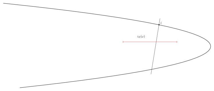
Figure 7: Long escape situation for the second critical point

5 Construction of a tangency

We aim to construct a non-degenerate quadratic tangency at the long escape time $\tilde{N}$. We consider a parameter interval $\tilde{\omega}$. For each $a$ in $\tilde{\omega}$ there is a critical point $\tilde{z}_{0}$ and a fixed point $\hat{z}_{a}$ For each fixed $a\in\tilde{\omega}$ a segment $\gamma_{u}^{a}\subset W^{u}(\hat{z}_{a})$ which contains $\tilde{z}_{a}$ and $\hat{z}_{a}$. We aim to prove that $F_{a}^{\tilde{N}}(\gamma_{u}^{a})$ has very high curvature near $F_{a}^{\tilde{N}}(\tilde{z}_{0}(a))$. It is advantageous to study the curvature of $F_{a}^{\tilde{N}-1}(\tilde{\gamma}_{u}^{a})$ where $\tilde{\gamma}_{u}^{a}$ is the curve $F_{a}(\gamma_{u}^{a})$ which is located close to the critical value.

We decompose the tangent vector $\tau(u)$ along $\tilde{\gamma}_{u}^{a}$ as

$$\tau(u)=A(u)E_{\tilde{N}-1}(u)+B(u)W_{\tilde{N}-1}(u)$$

where

$$\left\{\begin{matrix}E_{\tilde{N}-1}(u)=e_{\tilde{N}-1}(\zeta_{1}(u))\\ W_{\tilde{N}-1}(u)=DF_{a}^{\tilde{N}-1}(\zeta_{1}(u))\left(\begin{matrix}1\\ 0\end{matrix}\right)\end{matrix}\right.$$

and $\zeta_{1}(u)$ is the parametrization of $\tilde{\gamma}_{u}^{a}$ by arclength.

We have

$$\zeta_{\tilde{N}}(\rho)-\tilde{z}_{\tilde{N}}=\int_{0}^{\rho}\left(A(u)E_{\tilde{N}-1}(u)+B(u)W_{\tilde{N}-1}(u)\right)du.$$ (5.1)

Here $\zeta_{1}=\zeta_{1}(\rho)$ is an arbitrary point on $\tilde{\gamma}_{a}^{u}$ at arclength $\rho$ from $\tilde{z}_{1}(a)$ and $\zeta_{\tilde{N}}(\rho)=F_{a}^{\tilde{N}-1}\left(\zeta_{1}(\rho)\right)$.

Differentiating (5.1) twice, we get

$$\zeta^{\prime}_{\tilde{N}}(\rho)=A(\rho)E_{\tilde{N}-1}(\rho)+B(\rho)W_{\tilde{N}-1}(\rho)$$ (5.2)

and

$$\zeta^{\prime\prime}_{\tilde{N}}(\rho)=A^{\prime}(\rho)E_{\tilde{N}-1}(\rho)+A(\rho)E^{\prime}_{\tilde{N}-1}(\rho)+B^{\prime}(\rho)W_{\tilde{N}-1}(\rho)+B(\rho)W^{\prime}_{\tilde{N}-1}(\rho)$$ (5.3)

Lemma 5.4.

For all $\rho>0$

$$\left|W^{\prime}_{\tilde{N}-1}(\rho)\right|\leq 25^{\tilde{N}-1}.$$

Proof.

Observe that

$$W_{\tilde{N}-1}(\rho)=DF(x_{\tilde{N}-1},y_{\tilde{N}-1})\dots DF(x_{1},y_{1})\bigl{(}\begin{smallmatrix}1\\ 0\end{smallmatrix}\bigr{)}.$$

By differentiating with respect to $\rho$ and taking the matrix norm, one gets,

$$\left|W^{\prime}_{\tilde{N}-1}(\rho)\right|=\sum_{i}\left(\prod_{j\neq i}\left\|DF(x_{j},y_{j})\right\|\right)\left\|P_{i}\right\|$$

where

$$P_{i}=\frac{d}{d\rho}\left[\begin{matrix}-2ax_{i}+\partial_{x}\psi_{1}&\partial_{y}\psi_{1}\\ \partial_{x}\psi_{2}&\partial_{y}\psi_{2}\end{matrix}\right].$$

Since the $C^{2}$ norms of $\psi_{1}$ and $\psi_{2}$ have the bound $Cb^{t/2}$, see [MV], Section 7A, we get

$$\left|W^{\prime}_{\tilde{N}-1}(\rho)\right|\leq\sum_{i}\left[\left(\frac{9}{2}\right)^{\tilde{N}-2}\cdot 3\left(\frac{9}{2}\right)^{i}\right]\leq 25^{\tilde{N}}$$

where we used that $\left\|W_{i}\right\|<\left(\frac{9}{2}\right)^{i}$ (since $\left\|DF\right\|<\frac{9}{2}$). ∎

Proposition 5.5.

Let $|\rho_{0}|=\frac{\left|E_{\tilde{N}}(0)\right|}{\left\|W_{\tilde{N}}(0)\right\|}$, then for a suitably chosen $\rho^{\prime}_{0}$, and for all $\rho^{\prime}_{0}\leq|\rho|\leq\rho_{0}$, the curvature of $\zeta_{\tilde{N}}(\rho)$, $\kappa\left(\zeta_{\tilde{N}}(\rho)\right)$ satisfies the following:

$${2C_{1}}\frac{|W_{\tilde{N}}(\rho)|}{|E_{\tilde{N}}(\rho)|^{2}}\geq\kappa\left(\zeta_{\tilde{N}}(\rho)\right)\geq\frac{C_{1}}{2}\frac{|W_{\tilde{N}}(\rho)|}{|E_{\tilde{N}}(\rho)|^{2}}$$

with $2\leq C_{1}\leq 4$.

Remark 5.6.

Observe that the numbers $\frac{1}{2}$ and 2 appearing in the curvature estimates above can be chosen arbitrarily close to 1, if $b$ is sufficiently small.

Proof.

Recall that

$$\kappa(\rho)=\frac{\left|\zeta^{\prime}_{\tilde{N}}(\rho)\times\zeta^{\prime\prime}_{\tilde{N}}(\rho)\right|}{\left|\zeta^{\prime}_{\tilde{N}}(\rho)\right|^{3}}.$$

We start by computing $\zeta^{\prime}_{\tilde{N}}(\rho)\times\zeta^{\prime\prime}_{\tilde{N}}(\rho)$. We get

$$\zeta^{\prime}_{\tilde{N}}(\rho)\times\zeta^{\prime\prime}_{\tilde{N}}(\rho) = A(\rho)A^{\prime}(\rho)E_{\tilde{N}-1}(\rho)\times E_{\tilde{N}-1}(\rho)+A(\rho)^{2}E_{\tilde{N}-1}(\rho)\times E^{\prime}_{\tilde{N}-1}(\rho)$$

$$+ A(\rho)B^{\prime}(\rho)E_{\tilde{N}-1}(\rho)\times W_{\tilde{N}-1}(\rho)+A(\rho)B(\rho)E_{\tilde{N}-1}(\rho)\times W^{\prime}_{\tilde{N}-1}(\rho)$$

$$+ A^{\prime}(\rho)B(\rho)W_{\tilde{N}-1}(\rho)\times E_{\tilde{N}-1}(\rho)+A(\rho)B(\rho)W_{\tilde{N}-1}(\rho)\times E^{\prime}_{\tilde{N}-1}(\rho)$$

$$+ B(\rho)B^{\prime}(\rho)W_{\tilde{N}-1}(\rho)\times W_{\tilde{N}-1}(\rho)+B(\rho)^{2}W_{\tilde{N}-1}(\rho)\times W^{\prime}_{\tilde{N}-1}(\rho)$$

and since $E_{\tilde{N}-1}(\rho)\times E_{\tilde{N}-1}(\rho)=W_{\tilde{N}-1}(\rho)\times W_{\tilde{N}-1}(\rho)=0$

$$\zeta^{\prime}_{\tilde{N}}(\rho)\times\zeta^{\prime\prime}_{\tilde{N}}(\rho) = \left(A(\rho)B^{\prime}(\rho)-A^{\prime}(\rho)B(\rho)\right)E_{\tilde{N}-1}(\rho)\times W_{\tilde{N}-1}(\rho)$$

$$+ A(\rho)^{2}E_{\tilde{N}-1}(\rho)\times E^{\prime}_{\tilde{N}-1}(\rho)+B(\rho)^{2}W_{\tilde{N}-1}(\rho)\times W^{\prime}_{\tilde{N}-1}(\rho)$$

$$+ A(\rho)B(\rho)E_{\tilde{N}-1}(\rho)\times W^{\prime}_{\tilde{N}-1}(\rho)+A(\rho)B(\rho)W_{\tilde{N}}(\rho)\times E^{\prime}_{\tilde{N}-1}(\rho).$$

In [BC2], Section 7.5 there are estimates of $A$, $A^{\prime}$, $B$ and $B^{\prime}$ in the classical Hénon case. We have new similar estimates in the Hénon-like case as follows:

Claim.

There are constants $\gamma_{1}$ and $C_{1}=2a/\gamma_{0}^{2}$ such that

$$\frac{2}{\gamma_{0}^{2}}\rho\leq B(\rho) \leq\frac{4}{\gamma_{0}^{2}}\rho,$$ (5.7)

$$B^{\prime}(\rho) = \frac{2a}{\gamma_{0}^{2}}\frac{dy}{d\rho}+O(b)=C_{1}+O(b),$$ (5.8)

$$A(\rho) = 1+O(\rho^{2}),$$ (5.9)

$$A^{\prime}(\rho) = O(\rho).$$ (5.10)

We prove now the previous Claim. Observe that for $(x,y)$ close to the critical value $\tilde{z}_{1}$

$$Df_{a}=\left(\begin{matrix}-2ax+\psi_{1x}&\psi_{1y}\\ \psi_{2x}&\psi_{2y}\end{matrix}\right)=\left(\begin{matrix}-2ax+\alpha_{1}&\beta_{1}\\ \gamma_{1}&\delta_{1}\end{matrix}\right)$$

and

$$Df_{a}^{-1}=\frac{1}{\text{det}Df_{a}}\left(\begin{matrix}\delta_{1}&-\beta_{1}\\ -\gamma_{1}&-2ax+\alpha_{1}\end{matrix}\right).$$

It follows that

$$(Df_{a}^{-1})^{2}\left(\begin{matrix}.0\\ 1\end{matrix}\right)=\frac{1}{(\text{det}Df_{a})^{2}}\left(\begin{matrix}-\delta\beta_{1}-\beta_{1}(-2ax+\alpha_{1})\\ \beta_{1}\gamma_{1}+(-2ax+\alpha_{1})^{2}\end{matrix}\right)$$

This means that the most contractive direction for $(x,y)$ close to $\tilde{z}_{1}(a)$ has slope

$$s\approx\frac{2ax-\alpha_{1}}{\beta_{1}}.$$

By the construction of the local stable manifold, see [BC2] pp. 110-111, it follows that there is a temporary stable foliation with slope of $\approx{2ax_{1}}/{\beta}$ with $x_{1}\approx 1$.

We claim that the image of the leg of the unstable manifold near the critical value is an approximate parabola. The unstable direction at $\hat{z}$ is given by the unstable direction of the fixed point located approximately at $\left(\begin{matrix}1/2\\ 0\end{matrix}\right)$. The slope of $W^{u}$ near $\tilde{z}_{0}$ is given by

$$\left(\begin{matrix}-2ax_{-1}+\alpha_{-1}&\beta_{-1}\\ \gamma_{-1}&\delta_{-1}\end{matrix}\right)\left(\begin{matrix}-2ax_{-2}+\alpha_{-2}&\beta_{-2}\\ \gamma_{-2}&\delta_{-2}\end{matrix}\right)\dots\left(\begin{matrix}-2ax_{-k}+\alpha_{-k}&\beta_{-k}\\ \gamma_{-k}&\delta_{-k}\end{matrix}\right)v_{0}$$

where $v_{0}$ is the slope of $W^{u}(\hat{z})$ which is essentially horizontal. Observe that $x_{-1}$ is approximately given by $1-ax_{-1}^{2}=0$. The slope of $W^{u}$ near $\tilde{z}_{0}$ is approximately given by ${\gamma_{-1}}/{-2ax_{-1}}$.

By approximating the unstable manifold by a straight line

$$\begin{cases}x=x_{0}+t\\ y=y_{0}+kt\end{cases}$$

where $k={\gamma_{-1}}/{-2ax_{-1}}$ we have that the image of $W^{u}$ is the curve $(x_{1}(t),y_{1}(t)$ with the derivative

$$\begin{cases}x_{1}^{\prime}(t)=-2a(t+x_{0})+\alpha_{0}+k\beta_{0}\\ y_{1}^{\prime}(t)=\gamma_{0}+k\delta_{0}\end{cases}$$

so The curvature is then given by $\kappa(t)=|\gamma_{1}^{\prime}(t)\times\gamma_{2}^{\prime\prime}(t)|/|\gamma_{1}^{\prime}(t)|^{3}\approx 2a/\gamma_{0}^{2}$.

This means that, in a suitable almost orthogonal coordinate system $(\eta_{1},\xi_{1})$, one can use a version of Hadamard’s lemma, see Lemma 8.7 in [BC2] to get that the image parabola looks approximately as

$$\xi_{1}=1-a\left(\frac{\eta_{1}}{\gamma_{0}}\right)^{2}.$$

For convenience of the reader we recall here Lemma 8.7,[BC2] which we just used. Let $f\in C^{2}(A,A+\ell)$ and suppose that

$$|f(a)|\leq M_{0},\qquad|f^{\prime\prime}(a)|\leq M_{2}.$$

Then if

$$4M_{0}<\ell^{2}$$

it hold that

$$|f^{\prime}(a)|\leq\sqrt{M_{0}}(1+M_{2}).$$

This completes the proof of the Claim.

The following estimates hold.

$$\left|\left(A(\rho)B^{\prime}(\rho)-A^{\prime}(\rho)B(\rho)\right)E_{\tilde{N}-1}(\rho)\times W_{\tilde{N}-1}(\rho)\right| \geq \frac{3}{4}C_{1}\left|E_{\tilde{N}-1}(\rho)\times W_{\tilde{N}-1}(\rho)\right|$$

$$\geq \frac{C_{1}}{2}\left|E_{\tilde{N}-1}(\rho)\right|\left|W_{\tilde{N}-1}(\rho)\right|,$$

where we used the fact that the angle between $W_{\tilde{N}-1}$ and $E_{\tilde{N}-1}$ is very close to $\pi/2$l, see formula $(9)$, Section $6$ in [MV]. By Lemma $6.8$ in [MV], we get

$$\left|E_{\tilde{N}-1}(\rho)\times E^{\prime}_{\tilde{N}-1}(\rho)\right| \leq \left|E_{\tilde{N}-1}(\rho)\right|\left|E^{\prime}_{\tilde{N}-1}(\rho)\right|$$

$$\leq \left|E_{\tilde{N}-1}(\rho)\right|\left(K_{1}b\right)^{\tilde{N}-4}$$

with $K_{1}>0$. By Lemma 5.4 we have

$$\left|B(\rho)^{2}W_{\tilde{N}-1}(\rho)\times W^{\prime}_{\tilde{N}-1}(\rho)\right| \leq \left|W_{\tilde{N}-1}(\rho)\right|\frac{4^{2}}{\gamma_{0}^{2}}\rho^{2}25^{\tilde{N}-1}$$

$$\leq \left|W_{\tilde{N}-1}(\rho)\right|\left|E_{\tilde{N}-1}(\rho)\right|\cdot\frac{16}{\gamma_{0}^{2}}\left(\frac{\left|E_{\tilde{N}-1}(\rho_{0})\right|^{2}}{\left|W_{\tilde{N}-1}(\rho_{0})\right|^{2}|E_{\tilde{N}-1}(\rho)|}25^{\tilde{N}-1}\right)$$

$$\leq \frac{1}{100}\left|W_{\tilde{N}-1}(\rho)\right|\left|E_{\tilde{N}-1}(\rho)\right|,$$

. We have used the distorsion estimate for $W$-vectors, see [MV], Lemma 10.2. to conclude that $W_{\tilde{N}-1}(\rho)$ and $W_{\tilde{N}-1}(\rho_{0})$ are comparable, the estimate that $|W_{\tilde{N}-1}(\rho)|\cdot|E_{\tilde{N}-1}(\rho)|\approx b^{t(\tilde{N}-1)}$ and the estimate $\left|E_{\tilde{N}-1}(\rho)\right|<\left({Kb}/{\kappa}\right)^{\tilde{N}-1}$

By Lemma $6.8$ in [MV],

$$\left|A(\rho)B(\rho)W_{\tilde{N}-1}(\rho)\times E^{\prime}_{\tilde{N}-1}(\rho)\right| \leq \frac{8}{\gamma_{0}^{2}}|\rho|\left|W_{\tilde{N}-1}(\rho)\right|\left(K_{1}b\right)^{\tilde{N}-4}$$

$$\leq \frac{8}{\gamma_{0}^{2}}\frac{\left|E_{\tilde{N}-1}(\rho_{0})\right|}{\left|W_{\tilde{N}-1}(\rho_{0})\right|}\left|W_{\tilde{N}-1}(\rho_{0})\right|\left(K_{1}b\right)^{\tilde{N}-2}$$

$$\leq \frac{1}{100}\left|E_{\tilde{N}-1}(\rho_{0})\right|\left|W_{\tilde{N}-1}(\rho_{0})\right|.$$

By Lemma 5.4 we have

$$\left|A(\rho)B(\rho)E_{\tilde{N}-1}(\rho)\times W^{\prime}_{\tilde{N}-1}(\rho)\right| \leq \frac{8}{\gamma_{0}^{2}}|\rho|\left|E_{\tilde{N}-1}(\rho)\right|25^{\tilde{N}-1}$$

$$\leq \frac{8}{\gamma_{0}^{2}}\left|W_{\tilde{N}-1}(\rho_{0})\right|\left|E_{\tilde{N}-1}(\rho_{0})\right|\frac{\left|E_{\tilde{N}-1}(\rho_{0})\right|}{\left|W_{\tilde{N}-1}(\rho_{0})\right|^{2}}25^{\tilde{N}-1}$$

$$\leq \frac{1}{100}\left|W_{\tilde{N}-1}(\rho_{0})\right|\left|E_{\tilde{N}-1}(\rho_{0})\right|,$$

where we used that $|\rho|^{2}\leq|\rho_{0}|^{2}={\left|E_{\tilde{N}}(\rho_{0})\right|^{2}}/{\left|W_{\tilde{N}}(\rho_{0})\right|^{2}}$ and $\left|E_{\tilde{N}-1}(\rho)\right|<\left({Kb}/{\kappa}\right)^{\tilde{N}-1}$, $K,\kappa>0$, see formula $(5)$ of Section $6$ in [MV].

The term that dominates is $A(\rho)B^{\prime}(\rho)E_{\tilde{N-1}}(\rho)\times W_{\tilde{N-1}}(\rho)$. The proof of the lemma is concluded by combining the previous five estimates. ∎

5.1 Quadratic Tangency

We prove that in a long escape situation a quadratic tangency appears.

Proposition 5.11.

Let $z_{E}(\omega)$ be a curve segment of critical values in an escape situation that intersect $\gamma^{s}$, the leg of $W^{s}(\hat{z})$ pointing downwards. Then there exists a unique $a_{0}\in\omega$ such that the tangency between $\gamma^{s}_{a_{0}}$ and $\gamma^{u}_{a_{0}}$ is quadratic.

Remark 5.12.

Actually, the curvature of $\gamma^{s}_{a_{0}}$ is close to zero while the curvature of $\gamma^{u}_{a_{0}}$ is close to its maximal which is $2\frac{|W_{N}|}{|E_{N}|^{2}}$ within a factor close to $1$.

Proof.

By Proposition 5.5, the $\rho$ which makes the slope equal to $-{C}/{\sqrt{b}}$ is roughly

$$\rho=-\frac{|E_{N}|}{2C|W_{N}|}\sqrt{b}.$$

Observe that this $\rho$ satisfies the estimate $|\rho|\geq\rho_{0}$, so we avoid the exact tip of the parabola like image of the unstable manifold. We use the bounds in Proposition 5.5for the curvature and the angle between $E_{\tilde{N}}(0)$ and $W_{\tilde{N}}(0)$ is $\frac{\pi}{2}$. Using that $||W_{\tilde{N}}||\leq 25^{\tilde{N}}$ (Lemma 5.4) and $||DE_{\tilde{N}}||\leq C\sqrt{b}$ ([MV], Lemma 6.6), the statement follows.

∎

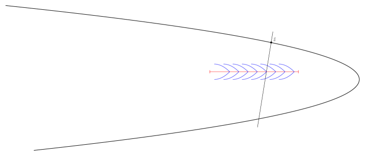
Figure 8: Quadratic tangency

6 Proof of theorems 1.3, 1.4 and 1.5

The proof of theorems 1.3, 1.4 and 1.5 is done by induction. From sections 3 and 5 we selected maps with a sink and a new tangency. We reapply now Section 3 to get a second sink and Section 5 to get a new tangency. One could stop this process after $k$ steps. At this moment one would have $k$ sinks and a new tangency. This tangency will then be used to create a strange attractor using [MV] and give the proof of Theorem 1.3. Alternatively, one could continue the process infinitely many times to get infinitely many sinks. This leads to the proof of Theorem 1.4. The inductive procedure is formulated in the next proposition.

Proposition 6.1.

There exists $K>0$ such that, for all $k=0,1,\dots,K$, there are parameters intervals $\omega_{k}$ with $\omega_{k}\subset\omega_{k-1}$, so that, for all $a\in\omega_{k}$, there is a $\mathcal{C}^{2}(b)$ curve $\gamma_{k}(a)\subset W^{u}(\hat{z})$ with $z_{k}(a)\in\gamma_{k}(a)$. Moreover, for all $k=0,1,\dots,K$ there are regions $\mathcal{D}_{N_{k}}(a)$ with $\mathcal{D}_{N_{j}}(a)\cap\mathcal{D}_{N_{i}}(a)=\emptyset$ for all $i\neq j$ such that $\mathcal{D}_{N_{k}}(a)$ is bounded by $\gamma_{k}(a)$ and parabolic leaves of $W^{s}_{\text{loc}}$ and it contains a unique sink.

Proof.

We proceed by induction and the case of one sink appears in Section 3. Assume that we have already constructed $k$ sinks and that a parameter interval $\omega^{(k)}$ corresponding to the critical point $z^{(k+1)}_{0}$ is in escape situation and intersects $W^{s}(\hat{z})$. We now have an unfolding of a homoclinic tangency as in Palis-Takens [PT] and [MV]. We can then do the renormalization procedure associated to this unfolding as in these papers and we obtain a new renormalized Hénon-like family. This allows us to create a new sink as in Section 3, and we obtain also a new escape situation following the argument in Section 4. ∎

Proof of Theorem 1.3. The proof is a small modification of that of Proposition 6.1. The only difference is that, at the time $k$, instead of construct a new sink one can create a strange attractor as in [MV] at the homoclinic unfolding.  $\square$

Proof of Theorem 1.4. The proof is a minor modification of that of Theorem 1.3. The only difference is that instead of switching to construction of a strange attractor after $k$ steps, we continue to construct more and more sinks. We obviously obtain Newhouse parameters in the limit. Note that the renormalizations take parameters of a specific Hénon-like family linearly to new renormalized parameters of the corresponding Hénon-like family. For each renormalization of order $k$, we get a set $A^{\prime}_{k}$ of parameters in the renormalized Hénon-like family of maps with $k$ sinks. We denote by $A_{k}$ the pullback of $A^{\prime}_{k}$ containing parameters of the original Hénon-like family. Consider now a non-empty closed subset of $A_{k}$, $B_{k}$ and denote by $B^{\prime}_{k}$ the push-forward of $B_{k}$. We do at this point, another renormalization and we get a sequence of inclusions

$$A_{1}\supset B_{1}\supset\dots\supset A_{k}\supset B_{k}\supset A_{k+1}\supset\dots.$$

The intersection

$$\bigcap_{k=1}^{\infty}A_{k}$$

is then non-empty and so is then the set of maps with infinitely many sinks.

 $\square$

Proof of Theorem 1.5. This result is a direct consequence of Theorem 1.3 and Theorem 1.4, since the Hénon family is a special example of a Hénon-like family.  $\square$

7 Construction of two coexisting strange attractors

In this section we prove the existence of two strange attractors for a parameter set of positive Lebesgue measure within the classical Hénon family.

We first outline the proof. The idea is to find parameters with two coexisting homoclinic tangencies. To do this we consider two very close critical points which are in escape situation simultaneously. We must chose them very carefully so that their images are at suitable distance at the escape situation. To do this we have to chose carefully their initial distance and the time they spend in the hyperbolic region outside of $(-\delta,\delta)$. We will create one true tangency for the first critical point at the point $a_{0}$ and then we create a tangency for a second critical point but for a different parameter value $a_{0}^{\prime}$. Both critical points will have associated parameter sets of positive one-dimensional Lebesgue measure with different strange attractors. These parameter sets will intersect if the parameters with the respective strange attractor are abundant at the respective points.

We return to the construction of the first critical point $z_{0}$ and the corresponding long escape situation of Section 3.1. We fix $b<b_{0}$ and by Lemma 3.2 we see that there is a subinterval $\tilde{\omega}_{0}$ such that $z_{E}(\tilde{\omega}_{0})$ is in a long escape situation.

We now construct a second critical point $\tilde{z}_{0}$. The construction is similar to the corresponding one in Section 4. The difference is that $\tilde{z}_{0}$ will be chosen much closer to $z_{0}$ vertically than $\tilde{z}_{0}$ is to $z_{0}$ and its distance can be chosen exponentially well spaced, see (4.2). From Lemma 4.1, choose $j$ and the corresponding $\hat{z}_{0}$ so that $j$ is the minimal integer so that for all $a\in\tilde{\omega}_{0}$ at time $E$, $\tilde{z}_{E}$ is still bound to $z_{E}$.

7.1 Proof of Theorem 1.6

We start with the construction of the first critical point $z_{0}$ and follow it until the first escape situation which appears at time $T_{0}$.

Close to $z_{0}$ we have a number of critical points which are inter-spaced as follows.

Proposition 7.1.

Close to the critical point $z_{0}$ we have a sequence of critical points $\tilde{z}_{0}^{(j)}$ so that with $\lambda_{1}$ denoting the unstable eigenvalue,

$$|z_{0}-\tilde{z}_{0}^{(j)}|\leq C\left(\frac{b}{|\lambda_{1}|}\right)^{j}$$

and

$$C^{\prime}\frac{b}{|\lambda_{1}|}|\tilde{z}_{0}^{(j)}-\tilde{z}_{0}^{(j-1)}|\leq|\tilde{z}_{0}^{(j+1)}-\tilde{z}_{0}^{(j)}|\leq C^{\prime\prime}\frac{b}{|\lambda_{1}|}|\tilde{z}_{0}^{(j)}-\tilde{z}_{0}^{(j-1)}|.$$

Proof.

The stable manifold at the fixed point $\hat{z}$ intersects the first leg of the unstable manifold in a homoclinic point $z_{h}$. Segments around $z_{h}$ are captured towards $\hat{z}$ and by the Lambda lemma these segments are accumulated on the unstable manifold, in particular at $z_{0}$. The behaviour is dominated by the behaviour at the fixed point $\hat{z}$ and is dominated by the stable eigenvalue $\lambda_{2}=b/\lambda_{1}$. ∎

We want to chose a $j$ so that $\tilde{z}_{0}^{(j)}$ is a suitable distance to $z_{0}$ so that at an escape time $E$ booth the point $z_{0}$ and $\tilde{z}_{0}^{(j)}$ escapes.

Consider a subinterval $\omega$ in the parameter space that escapes at time $T_{0}$. We can accomplish that $|z_{0}(\omega)|\sim\frac{1}{10}$. Now chose a second critical point $\tilde{z}_{0}^{(j)}(a)$ for $a\in\omega$. Denote the initial distance between $z_{0}(a)$ and $\tilde{z}_{0}^{(j)}(a)$ for a fixed $a\in\omega$ by $d_{j}$. By Proposition 7.1 it follows that

$$d_{j}=\mathcal{O}\left(\frac{b}{|\lambda_{1}|}\right)^{j}.$$

It follows that at an escape time $T_{0}$

$$|z_{T_{0}}(a)-\tilde{z}_{T_{0}}^{(j)}(a)|\sim\left(\frac{b}{|\lambda_{1}|}\right)^{j}||W_{T_{0}}(a)||,$$

where $\sim$ denotes that the quotients of the two sides are bounded above and below with fixed constants.

We want to accomplish that at a suitable time $T_{0}+L$ there are simultaneous intersections of $z_{T_{0}+L}(\omega^{\prime})$ and $\tilde{z}_{T_{0}}^{(j)}(\omega^{\prime})$ with different legs of the stable manifold $W^{s}(\hat{z})$ for all $a\in{\omega^{\prime}}$. To achieve this we study the distribution of the vertical segments of $W^{s}$. We consider the tent map

$$y\mapsto 1-2|y|$$

which is conjugate to the full quadratic map

$$1-2x^{2}$$

The preimages of the fixed point $y=\frac{1}{3}$ of the tent map are located in

$$y_{k,\nu}=\frac{k}{3\cdot 2^{\nu}},\qquad k=-3\cdot 2^{\nu}-1,\dots,3\cdot 2^{\nu}+1.$$

These points correspond to $x_{k,\nu}=\sin\frac{\pi}{2}y_{k,\nu}$ and by continuity this is approximately true for all $a$ close to 2. To each $x_{\nu,k}$ there corresponds an almost vertical branch $\gamma_{k,\nu}$ of $W^{s}$ and, by chosing $j$ and $L$ appropriately, we will have the situation that $\tilde{z}_{0}^{(j)}(a_{0})$ is located between $\gamma_{k,\nu}$ and $\gamma_{k+1,\nu}$ for suitable chosen $k$ and $\nu$. This follows by the following argument. Suppose that for a given orbit $z_{E+j}(\omega^{\prime})$, $j\geq 0$, moves outside $(-\delta,\delta)\times{\mathbb{R}}$. Note that $||Df||\leq 5$. By Lemma 4.5 in [BC2] it follows that the slope $s_{T+j}$ of $w_{T_{0}+j}$ satisfies $|s_{T_{0}+j}|\leq b/\delta$ if we restrict to a suitable parameter interval $\omega^{\prime}$.

After restricting $\omega^{\prime}$ further if necessary we can obtain that for some $j=L$, say $z_{T_{0}+j}(\omega^{\prime})$, stretches across one $\gamma_{k,\nu}$ and the stable leg of $W^{s}(\hat{z})$. Denote the intersection points by $a_{0}^{\prime}$ and $a_{0}^{\prime\prime}$ respectively.

We will need information about the local behavior at the image. It follows from Propostion 5.5 that there are points of tangencies for parameters $\tilde{a}_{0}^{\prime}$, $\tilde{a}_{0}^{\prime\prime}]$ close to $a_{0}^{\prime}$ respectively.

Let us consider the homoclinic tangencies that appears in Proposition 5.11 for the parameters $as=\tilde{a}^{\prime}_{0}$ and $as=\tilde{a}^{\prime\prime}_{0}$ at time $T_{0}+L$

Suppose that the common tangency occurs for a parameter $a_{0}$. We consider the normalization argument in [PT].

The curvature is given, by

$$Q_{1}=\frac{|W_{N}^{1}(\rho)|}{|E_{N}^{1}|^{2}\left({1+\left(\frac{|B(\rho)||W_{N}^{1}|}{|E_{N}^{1}|^{2}}\right)^{2}}\right)^{3/2}}$$

The maps $\varphi_{\mu}^{N}$ are written in coordinates

$$(1+x,y)\mapsto(0,1)+(H_{1}(\mu,x,y),H_{2}(\mu,x,y))$$

with

$$H_{1}(\mu,x,y) =v\cdot x^{2}+\mu+wy+\tilde{H}_{1}(\mu,x,y)$$

$$H_{2}(\mu,x,y) =u\cdot y+\tilde{H}_{2}(\mu,x,y).$$

They define $N$ dependent on reparametrization of the parameter $\mu$ and a $\mu$-dependent change of coordinates renormalizations. The parameter renormalization is given by

$$\overline{\mu}=\sigma^{2N}\cdot\mu+w\cdot\kappa^{N}\cdot\sigma^{2N}-\sigma^{N}.$$

In the renormalized coordinates the parameter interval is $[\overline{\mu}^{\prime}_{0},2]$. We write

$$[\overline{\mu}^{\prime}_{0},2]=\bigcup_{r\geq r_{0}}J^{\prime}_{r}=J^{\prime}_{r,\ell}$$ (7.2)

with $J^{\prime}_{r,\ell}$ disjoint and $|J^{\prime}_{r,\ell}|=\frac{1}{r^{2}}|J_{r}^{\prime}|$.

We do a similar decompostion of $[\overline{\mu}^{\prime\prime}_{0},2]$.

$$[\overline{\mu}^{\prime\prime}_{0},2]=\bigcup_{r\geq r_{0}}J^{\prime\prime}_{r}=J^{\prime\prime}_{r,\ell}$$ (7.3)

To each of the decompostions (7.2) and (7.3) we get two decompostions

$$[\tilde{a}^{\prime}_{0,0},\tilde{a}_{0}^{\prime}]=\bigcup_{r\geq r_{0}}\omega^{\prime}_{r}=\omega^{\prime}_{r,\ell},$$ (7.4)

and

$$[\tilde{a}^{\prime\prime}_{0,0},\tilde{a}_{0}^{\prime\prime}]=\bigcup_{r\geq r_{0}}\omega^{\prime\prime}_{r}=\omega^{\prime\prime}_{r,\ell}.$$ (7.5)

There is a uniform distorsion bound for the parameter maps $a^{\prime}\mapsto\nu^{\prime}$ and $a^{\prime\prime}\mapsto\nu^{\prime\prime}$

For each $\omega=\omega_{r,\ell}^{\prime}$ we do the parameter selection to create a strange attractor as in [MV].

Let $n$ be an essential free return time and let $E_{n}(z_{0})$ be the set kept at time $n$ where we take into accont the parameter deletions because of the (BA) conditions and the large deviation estimate. By formula (1) in Section 12 in [MV] the measure of the deleted set $\omega\setminus E_{n}(\omega)$ satisfies

$$m(\omega\setminus E_{n}(\omega))\leq B_{0}e^{-\alpha_{0}n}m(\omega),$$ (7.6)

where $B_{0}$ and $\alpha_{0}$ depend on $K,\alpha,\beta$ and $\delta$ but not on $N$ and $b$.

We define

$$E_{n}(\omega)=E_{n-1}(\omega)\setminus\left(\bigcup_{z_{0}}(\omega\setminus E_{n}(z_{0}))\right).$$ (7.7)

The number of critical points is

$$\#C_{n}\leq 4\left(\frac{K}{\rho_{0}}\right)^{\theta n}$$

by Section 12 in [MV].

This leads to

$$m(E_{n-1}\setminus E_{n}) \leq 4B_{0}4\left(\frac{K}{\rho_{0}}\right)^{\theta n}e^{-\alpha_{0}n}m(\omega)$$

$$= 4B_{0}\left(\left(\frac{K}{\rho_{0}}\right)^{\theta}e^{-\alpha_{0}}\right)^{n}m(\omega)$$

$$\leq 4B_{0}e^{-\alpha_{0}n/2}m(\omega)$$

and

$$m(\bigcup_{n\geq N}(E_{n-1}\setminus E_{n}))\leq\sum_{n\geq N}4B_{0}e^{-\alpha_{0}n/2}m(\omega).$$ (7.8)

This means that for $N$ sufficiently large only a small proportion of $\omega$ will be deleted.

We now turn to the construction of simultanous attractors.

The first attractor will be contructed as above and the second attractor will be chosen corresponding to intervals $\omega^{\prime\prime}=\omega^{\prime\prime}_{r,\ell}$.

We now prove the coexistence of two attractors. To the critical point $z_{0}$ there corresponds a parameter interval $\Omega_{0}=[{a}_{0,0}^{\prime},{a}^{\prime}_{0}]$ and to $\tilde{z}_{0}$ there corresponds the parameter interval $\Omega_{0}^{\prime\prime}=[a_{0,0}^{\prime\prime},a_{0}^{\prime\prime}]$. The subintervals $\omega^{\prime}_{r^{\prime},\ell^{\prime}}$ and $\omega^{\prime\prime}_{r^{\prime\prime},\ell^{\prime\prime}}$ will have intersections for suitable chosen $r^{\prime},\ell^{\prime},r^{\prime\prime},\ell^{\prime\prime}$, even for a number of adjacent $(r^{\prime},\ell^{\prime})$ and $\omega^{\prime\prime}_{r^{\prime\prime},\ell^{\prime\prime}}$. Because of the estimate (7.8) the corresponding sets $E^{\prime}_{r^{\prime},\ell^{\prime}}$ and $E^{\prime\prime}_{r^{\prime\prime},\ell^{\prime\prime}}$ will have a nonempty intersection.

We also have to verify that the two attractors are distict. This follows since the attractors can be chosen to be arbitrarily well localized and close to the different homoclinic tangencies.

We can now finish the proof of the main theorem of the section.

Proof of Theorem 1.6. Consider a $b$ interval $(b_{1},b_{2})$, $b_{2}>b_{1}>0$, and $b_{2}$ sufficiently small. For each $b\in(b_{1},b_{2})$ there is a set $E_{b}$ of positive Lebesgue measure so that there are two strange attractors and the result follows by Fubinis’ theorem.

References

- [BC1] Benedicks, M. and Carleson, L., On iterations of on , Ann. of Math. (2), 122, 1985, 1, 1-25.
- [BC2] Benedicks, M. and Carleson, L., The dynamics of the Hénon map, Ann. of Math. (2), 133, 1991, 1, 73–169.
- [BMP] Benedicks, M., Martens, M. and Palmisano, L., Newhouse Laminations, arXiv:1811.00617.
- [BV] Benedicks, M. and Viana, M., Solution of the basin problem for Hénon like attractors, Invent. math., 143, 2001, 375-434.
- [BY2] Benedicks, M. and Young, L.-S., Markov extensions and decay of correlations for certain Hénon maps, Astérisque, 261, 2000, xi,13-56.
- [BY1] Benedicks, M. and Young, L.-S., Sinai-Bowen-Ruelle measures for certain Hénon map, Invent. math., 112, 1993, 541-576.
- [Be] Berger, P., Abundance of non-uniformly hyperbolic Hénon like endomorphisms. arXiv:0903.1473.
- [Be1] Berger, P., Zoology in the Hénon family: twin babies and Milnor’s swallows, arXiv:1801.05628 .
- [GS] Gavrilov, N.K. and Silnikov, L.P., On the three dimensional dynamical system close to a system with a structually unstable homoclinic curve.. I. Math. USSR Sbornik, 17, 1972, 467-485; II. Math USSR Sbornik, 19, 1972, 139-156.
- [GST] Gonchenko, S., Shilnikov, L. and Turaev, D. On dynamical properties of multidimensional diffeomorphisms from Newhouse regions: I, Nonlinearity, 21, 2008, 923–972.
- [H] Hénon, M., A two dimensional mapping with a strange attractor, Comm. Math. Phys., 50, 1976, 1, 66-77.
- [MV] Mora, L. and Viana, M., Abundance of strange attractors, Acta Math., 171, 1993, 1-71.
- [N1] Newhouse, S., Diffeomorphisms with infinitely many sinks, Topology, 13, 1974, 9-18.
- [N2] Newhouse, S., The abundance of wild hyperbolic sets and non-smooth stable sets for diffeomorphisms, Publ. Math. IHES, 50, 1979, 101-151.
- [P] Palis, J. Jr., A global view of dynamics and a conjecture on the denseness of finitude of attractors, Astérisque, 261, 2000, 335-347.
- [PdMM] Palis, J. Jr., de Melo, W., Manning, A.K., Geometric Theory of Dynamical Systems An Introduction, 1982.
- [PT] Palis, J. and Takens, F., Hyperbolicity and sensitive chaotic dynamics at homoclinic bifurcations, Cambridge Studies in Advanced Mathematics, 35,1993, x+234.
- [Pal] Palmisano, L., Coexistence of non-periodic attractors, arXiv:1903.01446.
- [Ro] Robinson, Clark, Bifurcation to infinitely many sinks, Comm. Math. Phys., 90, 1983, 3, 433–459.
- [T] Thunberg, H., Unfolding of chaotic unimodal maps and the parameter dependence of natural measures, Nonlinearity (2), 14, 2001, 323–337.
- [U] Ures, Raúl, On the approximation of Hénon-like attractors by homoclinic tangencies., Ergodic Theory Dynam. Systems, 15, 1995, 1223-1229.
- [WY1] Wang, Q. and Young L.-S., Strange attractors with one direction of instability, Comm. Math. Phys., 218, 2001, 1–97.
- [WY2] Wang, Q. and Young L.-S., Towards a theory of rank one attractors, Ann of Math., 167, 2008, 349–480.