Abstract

Canonical variables for the Poisson algebra of quantum moments are introduced here, expressing semiclassical quantum mechanics as a canonical dynamical system that extends the classical phase space. New realizations for up to fourth order in moments for a single classical degree of freedom and to second order for a pair of classical degrees of freedom are derived and applied to several model systems. It is shown that these new canonical variables facilitate the derivation of quantum-statistical quantities and effective potentials. Moreover, by formulating quantum dynamics in classical language, these methods result in new heuristic pictures, for instance of tunneling, that can guide further investigations.

1 Introduction

Semiclassical physics can often be described by classical equations of motion amended by correction terms and possible new degrees of freedom. For instance, Ehrenfest’s theorem shows that the expectation values of position and momentum in an evolving quantum state obey equations of motion which are identical with the classical equations to zeroth order in $\hbar$ but, in general, have a modified quantum force given by $-\langle\nabla V(\hat{x})\rangle$ not equal to the classical force $-\nabla V(\langle\hat{x}\rangle)$ evaluated at $\langle\hat{x}\rangle$. The difference depends on $\langle\hat{x}\rangle$, but also on the variance $(\Delta x)^{2}$ and higher moments, which constitute new, non-classical degrees of freedom.

A moment expansion can be used to derive quantum corrections systematically. In this way, one can formulate quantum dynamics as classical-type dynamics on an extended phase space, given by expectation values and moments equipped with a Poisson bracket that follows from the commutator of operators [1, 2]. Moments, however, do not directly form canonical variables on this Poisson manifold, which complicates some of the usual procedures of canonical mechanics. Darboux’ theorem guarantees the existence of local canonical coordinates, but it is not always easy to find them. Using a procedure we developed in [3], as well as other new methods, we present here detailed derivations of canonical variables for moments of up to fourth order for a single degree of freedom, as well as to second order for a pair of degrees of freedom. The resulting expressions can be used to make interesting observations about the behavior of states, and they are crucial for the derivation of effective potentials. We present several applications, including tunneling which is also discussed in more detail in [4].

2 Canonical Effective Methods

We use a quantum system of $N$ degrees of freedom with basic operators $\hat{q}_{j}$ and $\hat{\pi}_{k}$, $1\leq j,k\leq N$ that are canonically conjugate,

$$[\hat{q}_{j},\hat{\pi}_{k}]=i\hbar\delta_{jk}\,.$$ (1)

In a semiclassical truncation [1, 2], the state space is described by a finite-dimensional phase space with coordinates given by the basic expectation values $q_{j}=\langle\hat{q}_{j}\rangle$ and $\pi_{k}=\langle\hat{\pi}_{k}\rangle$ and, for positive integers $k_{i}$ and $l_{i}$ such that $\sum_{i=1}^{N}(k_{i}+l_{i})\geq 2$, the moments

$$\Delta\left(q_{1}^{k_{1}}\cdots q_{N}^{k_{N}}\pi_{1}^{l_{1}}\cdots\pi_{N}^{l_{N}}\right)=\langle(\hat{q}_{1}-q_{1})^{{k_{1}}}\cdots(\hat{q}_{N}-q_{N})^{{k_{N}}}(\hat{\pi}_{1}-\pi_{1})^{{l_{1}}}\cdots(\hat{\pi}_{N}-\pi_{N})^{{l_{N}}}\rangle_{\mathrm{Weyl}}\,,$$ (2)

where the product of operators is Weyl (totally symmetrically) ordered. The phase-space structure is defined by the Poisson bracket

$$\{\langle\hat{A}\rangle,\langle\hat{B}\rangle\}=\frac{1}{i\hbar}\langle[\hat{A},\hat{B}]\rangle\,,$$ (3)

extended to all moments by using linearity and the Leibniz rule. The phase space has boundaries according to Heisenberg’s uncertainty relation

$$\Delta(q_{j}^{2})\Delta(\pi_{k}^{2})-\Delta(q_{j}\pi_{k})^{2}\geq\frac{\hbar^{2}}{4}\delta_{jk}$$ (4)

and higher-order analogs.

Any given state (which may be pure or mixed) is therefore represented by a point in phase space defined by the corresponding basic expectation values and moments. A state is considered semiclassical if its moments obey the hierarchy

$$\Delta\left(q_{1}^{k_{1}}\cdots q_{N}^{k_{N}}\pi_{1}^{l_{1}}\cdots\pi_{N}^{l_{N}}\right)=O\left(\hbar^{\frac{1}{2}\sum_{n}(l_{n}+k_{n})}\right)$$ (5)

which is satisfied, for instance, by a Gaussian, but includes also a more general class of states. A semiclassical truncation of order $s$ of the quantum system is defined as the submanifold spanned by the basic expectation values and moments such that $\sum_{n}(l_{n}+k_{n})\leq s$, which implies variables up to order $\frac{1}{2}s$ in $\hbar$ according to the semiclassical hierarchy. The Poisson bracket that results from (3) can consistently be restricted to any semiclassical truncation by ignoring in $\{\Delta_{1},\Delta_{2}\}$ all terms of order higher than $s$ in moments. In this restriction, the product of a moment of order $s_{1}$ and a moment of order $s_{2}$ is considered of semiclassical order $s_{1}+s_{2}$, while the product of a moment of order $s_{1}$ with $\hbar^{s_{2}}$ is of order $s_{1}+2s_{2}$ [5]. For given $s$, the Poisson tensor on the semiclassical truncation of order $s$ is, in general, not invertible. Therefore, semiclassical truncations and the resulting effective potentials cannot be formulated within symplectic geometry.

The Hamilton operator $\hat{H}$ determines a Hamilton function $\langle\hat{H}\rangle$ on state space, which can be restricted to any semiclassical truncation of order $s$ to define an effective Hamilton function of semiclassical order $s$. We assume that each contribution to the Hamilton operator is Weyl-ordered in basic operators. Any Hamilton operator that does not obey this condition can be brought to Weyl-ordered form by using the canonical commutation relations, which results in terms that explicitly depend on $\hbar$. In order to compute an effective Hamiltonian of order $s$ for a given Hamilton operator $H(\hat{q}_{j},\hat{\pi}_{k})$, we use

$$H_{{\rm eff},s} = \langle H(\hat{q}_{j}+(\hat{q}_{j}-q_{j}),\hat{\pi}_{k}+(\hat{\pi}_{k}-\pi_{k}))\rangle$$

$$= H(q_{j},\pi_{k})+\sum\limits_{\sum_{n}(j_{n}+k_{n})=2}^{s}\frac{\partial^{n}H(q,\pi)}{\partial q_{1}^{j_{1}}\cdots\partial q_{N}^{j_{N}}\partial\pi_{1}^{k_{1}}\cdots\partial\pi_{N}^{k_{N}}}\frac{\Delta\left(q_{1}^{j_{1}}\cdots q_{N}^{j_{N}}\pi_{1}^{k_{1}}\cdots\pi^{k_{N}}\right)}{j_{1}!\cdots j_{N}!k_{1}!\cdots k_{N}!}\,.$$

This expansion is reduced to a finite sum if $\hat{H}$ is polynomial in basic operators, in which case the expansion serves the purpose of expressing the expectation value of products of basic operators in terms of central moments. For a non-polynomial Hamilton operator, the expansion is a formal power series in $\hbar$. The definition of our Poisson bracket ensures that Hamilton’s equations

$$\dot{f}(\langle\cdot\rangle,\Delta)=\{f(\langle\cdot\rangle,\Delta),H_{{\rm eff,s}}\}$$ (7)

on any semiclassical truncation are consistent with Heisenberg’s equations of motion evaluated in a state.

2.1 Examples

For a single pair of classical degrees of freedom, $N=1$, the phase space of the semiclassical truncation of order two is five-dimensional (and therefore cannot be symplectic). In addition to the basic expectation values $q$ and $\pi$, there are two fluctuation variables, $\Delta(q^{2})$ and $\Delta(\pi^{2})$, and the covariance $\Delta(q\pi)$. The non-zero Poisson brackets of these variables are given by

$$\{q,\pi\} = 1$$ (8)

$$\{\Delta(q^{2}),\Delta(q\pi)\} = 2\Delta(q^{2})$$ (9)

$$\{\Delta(q\pi),\Delta(\pi^{2})\} = 2\Delta(\pi^{2})$$ (10)

$$\{\Delta(q^{2}),\Delta(\pi^{2})\} = 4\Delta(q\pi)$$ (11)

which are linear and equivalent to the Lie algebra ${\rm sp}(2,{\mathbb{R}})$.

More generally, the second-order semiclassical truncation for $N$ pairs of classical degrees of freedom is equivalent to ${\rm sp}(2N,{\mathbb{R}})$ [3]. Third-order semiclassical truncations also have linear Poisson brackets which are no longer semisimple: Within a higher-order semiclassical truncation, the Poisson bracket of two third-order moments is a sum of fourth-order moments and products of second-order moments, all of which are of order four and set to zero in a third-order truncation. Moreover, the Poisson bracket of a second-order moment and a third-order moment is proportional to a third-order moment, for instance

$$\{\Delta(q^{2}),\Delta(q^{2}\pi)\}=2\Delta(q^{3})\quad,\quad\{\Delta(q^{2}),\Delta(q\pi^{2})\}=4\Delta(q^{2}\pi)\quad,\quad\{\Delta(q^{2}),\Delta(\pi^{3})\}=6\Delta(q\pi^{2})$$ (12)

for $N=1$. The third-order moments in a semiclassical truncation of order three therefore form an Abelian ideal, and the corresponding Lie algebra is not semisimple. (For $N=1$, the Lie algebra is the semidirect product ${\rm sp}(2,{\mathbb{R}})\ltimes{\mathbb{R}}^{4}$ where ${\rm sp}(2,{\mathbb{R}})$ acts according to its spin-$3/2$ representation [3].)

For orders higher than three, the Poisson brackets are non-linear and therefore do not define Lie algebras. A general expression is given by [1, 6]

$$\{\Delta(q^{b}p^{a}),\Delta(q^{d}p^{c})\} = a\,d\,\Delta(q^{b}p^{a-1})\Delta(q^{d-1}p^{c})-bc\Delta(q^{b-1}p^{a})\Delta(q^{d}p^{c-1})$$ (13)

$$+\sum_{{\rm odd}\;n=1}^{M}\left(\frac{i\hbar}{2}\right)^{n-1}K_{abcd}^{n}\,\Delta(q^{b+d-n}p^{a+c-n})$$

where $M={\rm min}(a+c,b+d,a+b,c+d)$ and

$$K_{abcd}^{n}=\sum_{m=0}^{n}(-1)^{m}m!(n-m)!\left(\!\!\begin{array}[]{c}a\\ m\end{array}\!\!\right)\left(\!\!\begin{array}[]{c}b\\ n-m\end{array}\!\!\right)\left(\!\!\begin{array}[]{c}c\\ n-m\end{array}\!\!\right)\left(\!\!\begin{array}[]{c}d\\ m\end{array}\!\!\right)\,.$$ (14)

The inclusion of only odd $n$ in the sum ensures that all coefficients are real. Terms containing $\Delta(q)$ or $\Delta(p)$ are considered zero: They correspond to expectation values of the form $\langle\hat{a}-a\rangle=0$ which are identically zero.

2.2 Purity

The collection of all moments determines a state, provided it obeys conditions that follow from uncertainty relations. Since moments are defined using expectation values, which can be computed from a pure or mixed state, they may describe a pure or mixed state. In general, it is not easy to determine the purity of a state described by moments without first reconstructing a density matrix from them. As we will see, however, canonical variables for moments can provide indications as to possible impurity parameters. In preparation of this application, we discuss here ingredients for possible reconstructions of states from a given set of moments.

If the state is pure, it is sufficient to consider only the moments $\Delta(q^{n})$ and $\Delta(q^{n-1}\pi)$ to reconstruct a wave function [1]. For instance, we can use Hermite polynomials $H_{n}(q)$ and their coefficients $h_{n,l}$ defined such that $H_{n}(q)=\sum_{l}h_{n,l}q^{l}$. The expectation values $a_{n}=\langle\hat{q}^{n}\rangle$ can then be used to compute

$$c_{n}=\sum_{l}h_{n,l}a_{l}=\int{\rm d}q|\psi(q)|^{2}H_{n}(q)\,,$$ (15)

from which we obtain the probability density

$$|\psi(q)|^{2}=e^{-q^{2}}\sum_{n}\frac{c_{n}}{2^{n}\pi n!}H_{n}(q)$$ (16)

using the orthonormality relation of Hermite polynomials.

Using $b_{n}=\langle\hat{q}^{n}\hat{\pi}\rangle$, the phase $\alpha(q)$ of the wave function $\psi(q)=\exp(i\alpha(q))|\psi(q)|$ then follows from

$${\rm Re}b_{n} = {\rm Re}\int{\rm d}q\psi^{*}q^{n}\frac{\hbar}{i}\frac{{\rm d}\psi}{{\rm d}q}$$ (17)

$$= {\rm Re}\int{\rm d}qe^{-i\alpha}|\psi|q^{n}\frac{\hbar}{i}\left(i\frac{{\rm d}\alpha}{{\rm d}q}e^{i\alpha}|\psi|+e^{i\alpha}\frac{{\rm d}|\psi|}{{\rm d}q}\right)$$ (18)

$$= \hbar\int{\rm d}q|\psi|^{2}q^{n}\frac{{\rm d}\alpha}{{\rm d}q}\,.$$ (19)

If we define

$$d_{n}=\sum_{l}h_{n,l}{\rm Re}b_{n}=\hbar\int{\rm d}q|\psi|^{2}\frac{{\rm d}\alpha}{{\rm d}q}H_{n}(q)\,,$$ (20)

we reconstruct

$$\frac{{\rm d}\alpha}{{\rm d}q}=\frac{e^{-q^{2}}}{\hbar|\psi|^{2}}\sum_{n}\frac{d_{n}}{2^{n}\pi n!}H_{n}(q)\,.$$ (21)

Integration gives $\alpha(q)$ up to an arbitrary constant phase.

In order to reconstruct a density matrix, we need all moments. First, position moments are given by

$$\Delta(q^{a})={\rm tr}((\hat{q}-\langle\hat{q}\rangle)^{a}\hat{\rho})=\int(q-\langle\hat{q}\rangle)^{a}\rho(q,q){\rm d}q$$ (22)

from which we can reconstruct the diagonal part $\rho(q,q)$ using orthogonal polynomials. Using momentum-dependent moments, we can compute the values of

$${\rm tr}((\hat{q}-\langle\hat{q}\rangle)^{a}\hat{\pi}^{b}\hat{\rho})=\left(\frac{\hbar}{i}\right)^{b}\int(q-\langle\hat{q}\rangle)^{a}\left.\frac{\partial^{b}\rho(y,q)}{\partial y^{b}}\right|_{y=q}{\rm d}q$$ (23)

and use them in

$$\sum_{b}\frac{1}{b!}\left(\frac{id}{\hbar}\right)^{b}{\rm tr}((\hat{q}-\langle\hat{q}\rangle)^{a}\hat{\pi}^{b}\hat{\rho}) = \int(q-\langle\hat{q}\rangle)^{a}\sum_{b}\frac{d^{b}}{b!}\left.\frac{\partial^{b}\rho(y,q)}{\partial y^{b}}\right|_{y=q}{\rm d}q$$ (24)

$$= \int(q-\langle\hat{q}\rangle)^{a}\rho(q+d,q){\rm d}q$$

to reconstruct $\rho(q+d,q)$ for arbitrary $q$ and $d$.

In a semiclassical truncation we have incomplete information about the moments and it may be impossible to tell with certainty whether truncated moments correspond to a pure or mixed state. However, if there are parameters that appear only in moments of the form $\Delta(q^{a}\pi^{b})$ with $b>1$, they may be considered candidates for impurity parameters. We will see several examples in our derivation of canonical variables for moments.

2.3 Casimir–Darboux coordinates

Since the brackets (13) are non-canonical, it is not possible to interpret the moments directly in terms of configuration variables and momenta. However, the Darboux theorem and its generalization to Poisson manifolds guarantees that one can always choose coordinates that are canonical, together with a set of Casimir coordinates that have vanishing Poisson brackets with all other variables. The required transformation from moments to Casimir–Darboux variables of this form is, in general, non-linear. In [3], we have developed a systematic method to derive such transformations, based on a proof of Darboux’ theorem given in [7]. We have applied this method to semiclassical truncations in [3], which we review here with further details in the relevant integrations.

2.3.1 Single pair of degrees of freedom at second order

We illustrate the method for the case of a semiclassical truncation of order two for a single canonical pair of degrees of freedom. In this case, Casimir–Darboux variables had already been found independently in [8, 9].

The relevant Poisson brackets of second-order moments are given in (8). The procedure starts by choosing a function that plays the role of the first canonical coordinate. It is convenient to have a quantum fluctuation as one of the configuration variables, and therefore we choose $s=\sqrt{\Delta(q^{2})}$. This function, viewed formally as a Hamiltonian, is the generator of a Hamiltonian flow on phase space defined by

$$\frac{{\rm d}f(\Delta(q^{2}),\Delta(q\pi),\Delta(\pi^{2})}{{\rm d}\epsilon}=\{f(\Delta(q^{2}),\Delta(q\pi),\Delta(\pi^{2}),s\}\,.$$ (25)

If we already knew canonical coordinates, it would be obvious that the Poisson bracket on the right-hand side of this equation changes only the variable $p_{s}$ canonically conjugate to $s$, and therefore the derivative should be equal to the (negative) partial derivative of $f$ by $p_{s}$. Since we do not know $p_{s}$ yet, we revert this argument and implicitly define $p_{s}$ such that the derivatives in (25) equal the negative partial deirvative by $p_{s}$ for any function $f$. In particular, for the three second-order moments we obtain

$$\frac{\partial\Delta(q^{2})}{\partial p_{s}} = -\{\Delta(q^{2}),\sqrt{\Delta(q^{2})}\}=0$$ (26)

$$\frac{\partial\Delta(q\pi)}{\partial p_{s}} = -\{\Delta(q\pi),\sqrt{\Delta(q^{2})}\}=\sqrt{\Delta(q^{2})}=s$$ (27)

$$\frac{\partial\Delta(\pi^{2})}{\partial p_{s}} = -\{\Delta(\pi^{2}),\sqrt{\Delta(q^{2})}\}=2\frac{\Delta(q\pi)}{\sqrt{\Delta(q^{2})}}=2\frac{\Delta(q\pi)}{s}\,.$$ (28)

By construction, these are partial differential equations in which $s$ is held constant. We can easily solve (27) by

$$\Delta(q\pi)=sp_{s}+f_{1}(s)$$ (29)

with a free function $f_{1}$ depending only on $s$. Inserting this solution in (28), we have

$$\Delta(\pi^{2})=p_{s}^{2}+2\frac{f_{1}(s)}{s}p_{s}+f_{2}(s)$$ (30)

with another free function $f_{2}$ depending only on $s$.

Computing $\{\Delta(q\pi),\Delta(\pi^{2})\}$ using the canonical nature of the variables $s$ and $p_{s}$, and requiring that it equal $2\Delta(\pi^{2})$ implies two equations:

$$\frac{{\rm d}f_{1}}{{\rm d}s}=\frac{f_{1}}{s}\quad,\quad\frac{{\rm d}f_{2}}{{\rm d}s}=2\frac{f_{1}}{s^{2}}\frac{{\rm d}f_{1}}{{\rm d}s}-2\frac{f_{2}}{s}\,.$$ (31)

They are solved by

$$f_{1}(s)=U_{2}s\quad,\quad f_{2}(s)=\frac{U_{1}}{s^{2}}+U_{2}^{2}$$ (32)

with constants $U_{1}$ and $U_{2}$. We can eliminate $U_{2}$ by a canonical transformation replacing $p_{s}$ with $p_{s}+U_{2}$. The constant $U_{1}$ is the Casimir coordinate. The resulting moments in terms of Casimir–Darboux variables are

$$\Delta(q^{2})=s^{2}\quad,\quad\Delta(q\pi)=sp_{s}\quad,\quad\Delta(\pi^{2})=p_{s}^{2}+\frac{U_{1}}{s^{2}}$$ (33)

as in [8, 9].

In general, it may be difficult to recognize a variable such as $U_{1}$ as a Casimir coordinate. In such a case, the flow generated by $s$ or $s^{2}=\Delta(q^{2})$ is again useful:

$$\frac{{\rm d}\Delta(q\pi)}{{\rm d}\epsilon}=-2\Delta(q^{2})\quad,\quad\frac{{\rm d}\Delta(\pi^{2})}{{\rm d}\epsilon}=-4\Delta(q\pi)\,.$$ (34)

The solutions are similar to what we already used, $\Delta(q\pi)[\epsilon]=-2\Delta(q^{2})\epsilon+d$ for the first equation and $\Delta(\pi^{2})[\epsilon]=4\Delta(q^{2})\epsilon^{2}-4d\epsilon+e$ for the second equation, with constants $d$ and $e$. But now we use these equations to eliminate $\epsilon$ instead of solving for $p_{s}$. Inserting $\epsilon=\frac{1}{2}(d-\Delta(q\pi)[\epsilon])/s^{2}$ in $\Delta(\pi^{2})[\epsilon]$ implies

$$\Delta(\pi^{2})[\epsilon]=\frac{\Delta(q\pi)[\epsilon]^{2}}{\Delta(q^{2})}-3\frac{d^{2}}{\Delta(q^{2})}+e\,.$$ (35)

The combination $U_{1}=\Delta(q^{2})\Delta(\pi^{2})[\epsilon]-\Delta(q\pi)[\epsilon]^{2}=-3d^{2}+es^{2}$ is therefore independent of $\epsilon$. Since ${\rm d}U_{1}/{\rm d}\epsilon=\{U_{1},\Delta(q^{2})\}=0$, $U_{1}$ is a coordinate Poisson orthogonal to $s$. It is also Poisson orthogonal to $p_{s}$ by construction, and therefore represents the Casimir variable of this system.

2.3.2 Single pair of degrees of freedom at third order

We now try to find an extension of our Casimir–Darboux coordinates to third order. There are now seven moments, and the rank of the Poisson tensor shows that there is a single Casimir variable. We must therefore derive two additional pairs of canonical degrees of freedom. Since Darboux coordinates are defined only up to canonical transformations, the form in which they appear in the moments is not unique and subject to choices. For now, we make a choice motivated by the canonical form we just derived at second order: We assume that $\Delta(q^{2})$ depends only on one of the new canonical pairs,

$$\Delta(q^{2})=s_{1}^{2}$$ (36)

from which it quickly follows, by a calculation similar to our second-order example, that

$$\Delta(q\pi)=s_{1}\,p_{1}$$ (37)

is a consistent (but not unique) choice of introducing the first momentum.

The remaining canonical pairs must be such that they have zero Poisson brackets with $s_{1}$ and $p_{1}$, or with $\Delta(q^{2})$ and $\Delta(q\pi)$ according to our first choices. The same procedure that we used to derive $U_{1}$ as a coordinate Poisson orthogonal to both $s$ and $p_{s}$ at second order can also be used here, but now we have five additional moments which should be expressed in terms of functions Poisson orthogonal to $s$ and $p_{s}$. By systematically computing the flows of all the remaining moments generated by $s_{1}$ and $p_{1}$ and eliminating flow parameters, it follows that the following functions of moments are Poisson orthogonal to $s_{1}$ and $p_{1}$:

$$f_{1} = \Delta(q^{2})\Delta(\pi^{2})-\Delta(q\pi)^{2}$$

$$f_{2} = \Delta(q^{2})\frac{\Delta(q^{2}\pi)}{\Delta(q^{3})}-\Delta(q\pi)$$

$$f_{3} = \frac{\Delta(q^{2})^{2}}{\Delta(q^{3})^{2}}\left(\Delta(q^{2}\pi)^{2}-\Delta(q\pi^{2})\Delta(q^{3})\right)$$

$$f_{4} = 2\Delta(q\pi)+\Delta(q^{2})\frac{\Delta(q^{3})\Delta(\pi^{3})-\Delta(q\pi^{2})\Delta(q^{2}\pi)}{\Delta(q^{2}\pi)^{2}-\Delta(q\pi^{2})\Delta(q^{3})}\,.$$

One additional variable can be derived independently from the Casimir function of the Lie algebra that corresponds to third-order moments,

$$f_{5}:=U_{1}^{4} = \left(\Delta(q^{2}\pi)\Delta(q\pi^{2})-\Delta(q^{3})\Delta(\pi^{3})\right)^{2}$$ (39)

$$-4\left(\Delta(q\pi^{2})^{2}-\Delta(q^{2}\pi)\Delta(\pi^{3})\right)\left(\Delta(q^{2}\pi)^{2}-\Delta(q^{3})\Delta(q\pi^{2})\right)\,.$$

(The fourth power of $U_{1}$ is chosen such that $U_{1}$ is of third order just like the moment order considered here.) While $f_{5}$ Poisson commutes with all other $f_{i}$, $(f_{1},f_{2},f_{3},f_{4})$ have non-linear brackets

$$\left\{f_{1},f_{2}\right\} = 2f_{1}+2f_{2}^{2}+4f_{3}$$ (40)

$$\left\{f_{1},f_{3}\right\} = 12f_{2}f_{3}+2f_{3}f_{4}$$ (41)

$$\left\{f_{1},f_{4}\right\} = -4f_{1}-f_{4}^{2}+4f_{3}-\left(2f_{2}+f_{4}\right)^{2}$$ (42)

$$\left\{f_{2},f_{3}\right\} = -4f_{3}$$ (43)

$$\left\{f_{2},f_{4}\right\} = -4f_{2}-2f_{4}$$ (44)

$$\left\{f_{3},f_{4}\right\} = -8f_{3}$$ (45)

with one another.

We are now ready to choose our second configuration variable. We define

$$s_{2}=f_{3}\,,$$ (46)

such that

$$\frac{\partial f_{1}}{\partial p_{2}}=-12s_{2}f_{2}-2s_{2}f_{4}\quad,\quad\frac{\partial f_{2}}{\partial p_{2}}=4s_{2}\quad,\quad\frac{\partial f_{4}}{\partial p_{2}}=-8s_{2}$$ (47)

can be used to determine the second momentum variable. Integrating the last two equations and inserting the results in the first one gives

$$f_{1} = -16s_{2}^{2}p_{2}^{2}-s_{2}\left(12g_{2}+2g_{4}\right)p_{2}+g_{1}$$ (48)

$$f_{2} = 4s_{2}p_{2}+g_{2}$$ (49)

$$f_{4} = -8s_{2}p_{2}+g_{4}$$ (50)

with three functions $g_{1}$, $g_{2}$ and $g_{4}$ independent of $p_{2}$. (They can therefore depend on $s_{2}$ and the remaining canonical pair, $s_{3}$ and $p_{3}$, as well as the Casimir variable $U_{1}$.) Since we are interested in deriving $p_{2}$, we can choose the free functions such that it is easy to invert (48), (49) or (50) for $p_{2}$. A wrong choice at this point could result in a degenerate system that does not allow us to derive all canonical pairs. Since we know how many canonical pairs we obtain, a little bit of trial and error quickly shows when a choice is suitable. If we choose $g_{4}=-6g_{2}$, we obtain

$$p_{2}=\frac{6f_{2}+f_{4}}{16s_{2}}$$ (51)

from a combination of (49) and (50), as well as

$$g_{1}=f_{1}+\frac{\left(6f_{2}+f_{4}\right)^{2}}{16}\quad,\quad g_{2}=-\frac{1}{2}f_{2}-\frac{1}{4}f_{4}\,.$$ (52)

By construction, $g_{1}$ and $g_{2}$ do not depend on $p_{2}$, but we have not made sure yet that they do not depend on $s_{2}$ either. Since $s_{2}$ is defined as $s_{3}$, the Poisson brackets (40)–(45) can be used to show that $g_{1}$ and $g_{2}$ do, in fact, depend on $s_{2}$. The same Poisson brackets determine the canonical flow generated by $p_{2}$ in (51) on $g_{1}$ and $g_{2}$. By eliminating the flow parameter as in some of the previous steps, we find that the combinations

$$p_{3} = \frac{g_{2}}{\sqrt{s_{2}}}$$ (53)

$$s_{3} = \frac{2g_{1}-7s_{2}+10p_{3}^{2}s_{2}}{6\sqrt{s_{2}}(4p_{3}^{2}-1)}$$ (54)

are independent of $s_{2}$ and are therefore Poisson orthogonal to all previously constructed canonical pairs. They determine our final pair $(s_{3},p_{3})$.

In order to express moments in terms of canonical pairs and the Casimir variable, we insert the functions

$$f_{1} = 3\sqrt{s_{2}}\left(-1+4p_{3}^{2}\right)s_{3}+\frac{1}{2}\left(7s_{2}-10s_{2}p_{3}^{2}\right)-16s_{2}^{2}p_{2}^{2}$$ (55)

$$f_{2} = \sqrt{s_{2}}p_{3}+4s_{2}p_{2}$$ (56)

$$f_{3} = s_{2}$$ (57)

$$f_{4} = -4\sqrt{s_{2}}p_{3}-8s_{2}p_{2}$$ (58)

$$f_{5} = U_{1}^{4}$$ (59)

in (2.3.2) and (39) and invert the resulting relations for

$$\Delta(q^{2}) = s_{1}^{2}\quad,\quad\Delta(q\pi)=s_{1}p_{1}$$ (60)

$$\Delta(\pi^{2}) = p_{1}^{2}+\frac{f_{1}}{s_{1}^{2}}=p_{1}^{2}+\frac{3\sqrt{s_{2}}\left(4p_{3}^{2}-1\right)s_{3}+\frac{1}{2}s_{2}\left(7-10p_{3}^{2}\right)-16s_{2}^{2}p_{2}^{2}}{s_{1}^{2}}$$ (61)

$$\Delta(\pi^{3}) = \frac{U_{1}}{s_{1}^{3}\sqrt{2s_{2}^{3/2}\sqrt{1-4p_{3}^{2}}}}\Phi(s_{i},p_{i})$$ (62)

$$\Delta(q\pi^{2}) = \frac{U_{1}}{s_{1}\sqrt{2s_{2}^{3/2}\sqrt{1-4p_{3}^{2}}}}\left(p_{1}s_{1}+\left(p_{3}-1\right)\sqrt{s_{2}}+4s_{2}p_{2}\right)$$ (64)

$$\times\left(p_{1}s_{1}+\left(1+p_{3}\right)\sqrt{s_{2}}+4s_{2}p_{2}\right)$$

$$\Delta(q^{2}\pi) = \frac{U_{1}}{\sqrt{2s_{2}^{3/2}\sqrt{1-4p_{3}^{2}}}}\left(p_{1}s_{1}^{2}+s_{1}\left(p_{3}\sqrt{s_{2}}+4s_{2}p_{2}\right)\right)$$ (65)

$$\Delta(q^{3}) = \frac{U_{1}s_{1}^{3}}{\sqrt{2s_{2}^{3/2}\sqrt{1-4p_{3}^{2}}}}\,,$$ (66)

where

$$\Phi(s_{i},p_{i}) = p_{1}^{3}s_{1}^{3}+3p_{1}^{2}p_{3}s_{1}^{2}\sqrt{s_{2}}+3p_{1}s_{1}s_{2}\left(-1+p_{3}^{2}+4p_{1}s_{1}p_{2}\right)+64p_{2}^{3}s_{2}^{3}$$

$$+p_{3}s_{2}^{3/2}\left(-7+p_{3}^{2}+24p_{1}p_{2}s_{1}\right)+48p_{3}p_{2}^{2}s_{2}^{5/2}+12p_{2}s_{2}^{2}\left(-1+p_{3}^{2}+4p_{1}s_{1}p_{2}\right)\,.$$

More compactly, some of the momentum-dependent moments can be written as

$$\Delta(\pi^{3}) = \frac{U_{1}\left(P^{3}-3P-4p_{3}s_{2}^{3/2}\right)}{s_{1}^{3}\sqrt{2s_{2}^{3/2}\sqrt{1-4p_{3}^{2}}}}$$ (68)

$$\Delta(q\pi^{2}) = \frac{U_{1}\left(P^{2}-s_{2}\right)}{s_{1}\sqrt{2s_{2}^{3/2}\sqrt{1-4p_{3}^{2}}}}$$ (69)

$$\Delta(q^{2}\pi) = \frac{U_{1}s_{1}P}{\sqrt{2s_{2}^{3/2}\sqrt{1-4p_{3}^{2}}}}$$ (70)

if we introduce $P=p_{1}s_{1}+p_{3}\sqrt{s_{2}}+4s_{2}p_{2}$. Note that $s_{3}$ does not appear in any $\Delta(q^{a}\pi^{b})$ with $b\leq 1$, and may therefore be a candidate for the impurity of a state.

2.3.3 Third order by ansatz

As we have seen, several choices have to be made in the process of deriving Casimir–Darboux coordinates. Some choices may lead to degenerate systems in which a smaller number of canonical pairs results, and which should therefore be discarded. However, even within the class of non-degenerate systems, there cannot be a unique set of Casimir–Darboux coordinates because one can always apply canonical transformations of Darboux variables. Depending on the application, some choices may lead to more useful realizations of canonical variables than others. Staying with the third-order system for a single pair of canonical degrees of freedom, we now apply an alternative method which works by ansatz and therefore is somewhat less systematic than the previous procedure. However, it makes it easier to implement certain properties such as a simplified version of $\Delta(\pi^{2})$ in (61) with $s_{i}$-independent coefficients. As we will see, such a version greatly simplifies the effective dynamics, but it does not always exist, in particular if we have more than one pair of classical degrees of freedom.

We make the ansatz

$$\Delta(\pi^{2})=\sum_{i=1}^{3}p_{i}^{2}+F(s_{1},s_{2},s_{3})\quad \quad\Delta(q\pi)=\sum_{i=1}^{3}s_{i}p_{i}$$ , (71)

$$\Delta(q^{2})=\sum_{i=1}^{3}s_{i}^{2}\quad \quad\Delta(q^{3})=\sum_{i=1}^{3}s_{i}^{3}$$ , (72)

introducing three canonical pairs, as required. The function $F(s_{1},s_{2},s_{3})$, which is assumed to be independent of the momenta, is subject to consistency conditions that follow from the required Poisson brackets of moments. Once we have a consistent $F$, we can generate all the remaining moments by taking successive Poisson brackets with $\Delta(\pi^{2})$:

$$\Delta(q^{m-1}\pi^{n+1})=-\frac{1}{2m}\left\{\Delta(\pi^{2}),\Delta(q^{m}\pi^{n})\right\}\,,$$ (73)

starting with $m=3$, $n=0$ in which case we have defined $\Delta(q^{3})$ in (72) and can derive

$$\Delta(q^{2}\pi) = \sum_{i}p_{i}s_{i}^{2}$$ (74)

$$\Delta(q\pi^{2}) = \sum_{i}p_{i}^{2}s_{i}-\frac{1}{4}\sum_{i}s_{i}^{2}\frac{\partial F}{\partial s_{i}}$$ (75)

$$\Delta(\pi^{3}) = \sum_{i}p_{i}^{3}-\frac{1}{4}\sum_{i}p_{i}\left(4s_{i}\frac{\partial F}{\partial s_{i}}+\sum_{j}s_{j}^{2}\frac{\partial^{2}F}{\partial s_{i}\partial s_{j}}\right)\,.$$ (76)

Since we have explicitly used all three canonical pairs expected for a third-order truncation, $F$ depends on one further parameter, $U$, which will be the Casimir coordinate. Since $F$ and therefore $U$ appear only in moments which have at least two momentum factors, $U$ is a candidate for an impurity parameter in this mapping.

Equation (73) also applies to second-order moments, $m+n=2$. Since we have defined all three second-order moments in (71), we obtain consistency conditions on $F$. We first compute

$$\{\Delta(\pi^{2}),\Delta(q^{2})\}=-4\sum_{i}s_{i}p_{i}$$ (77)

and from this

$$\{\Delta{\pi^{2}},\{\Delta(\pi^{2}),\Delta(q^{2})\}\}=8\sum_{i}p_{i}^{2}-4\sum_{i}s_{i}\frac{\partial F}{\partial s_{i}}\,.$$ (78)

The condition

$$\{\Delta{\pi^{2}},\{\Delta(\pi^{2}),\Delta(q^{2})\}\}=8\Delta(\pi^{2})$$ (79)

then implies

$$\sum_{i}s_{i}\frac{\partial F}{\partial s_{i}}=-2F$$ (80)

and therefore $F$ is homogeneous of degree $-2$ if all $s_{i}$ are rescaled by the same constant.

Applying further Poisson brackets with $\Delta(\pi^{2})$ does not give new conditions. For instance,

$$0=\left\{\Delta(\pi^{2}),\left\{\Delta(\pi^{2}),\left\{\Delta(\pi^{2}),\Delta(q^{2})\right\}\right\}\right\}$$ (81)

is equivalent to

$$0=8\left(3\sum_{i}p_{i}\frac{\partial F}{\partial s_{i}}+\sum_{i,j}p_{i}s_{j}\frac{\partial^{2}F}{\partial s_{i}\partial s_{j}}\right)\,.$$ (82)

Since the $s_{i}$ and $p_{i}$ can be varied independently, the condition implies that all three $\partial F/\partial s_{i}$ are homogeneous of degree $-3$ if all $s_{i}$ are rescaled by the same constant, which follows from $F$ being of degree $-2$.

Another consistency condition can be derived by looking at the third order moments:

$$0=\left\{\Delta(\pi^{2}),\left\{\Delta(\pi^{2}),\left\{\Delta(\pi^{2}),\left\{\Delta(\pi^{2}),\Delta(q^{3})\right\}\right\}\right\}\right\}$$ (83)

is equivalent to

$$0 = 6\sum_{i}p_{i}^{2}\frac{\partial F}{\partial s_{i}}+4\sum_{ij}p_{i}s_{i}p_{j}\frac{\partial^{2}F}{\partial s_{i}\partial s_{j}}+\frac{1}{2}\sum_{ijk}s_{i}^{2}p_{j}p_{k}\frac{\partial^{3}F}{\partial s_{i}\partial s_{j}\partial s_{k}}$$ (85)

$$-\frac{3}{2}\sum_{i}s_{i}\left(\frac{\partial F}{\partial s_{i}}\right)^{2}-\frac{1}{4}\sum_{ij}s_{i}^{2}\frac{\partial F}{\partial s_{j}}\frac{\partial^{2}F}{\partial s_{i}\partial s_{j}}\,.$$

This condition is generally independent from (80). For example, the solution $F=\sum_{i}U/s_{i}^{2}$ of (80) is not a solution of (85).

One further condition has to be imposed, which is the invertibility of the mapping from moments to $(s_{i},p_{s_{j}})$. (Otherwise one could choose the trivial solution $F=0$.) For any given $F$, this condition can be checked by computing the Jacobian of the transformation, and it is fulfilled, for instance, by the solutions

$$F(s_{1},s_{2},s_{3})=\sum_{i<j}\frac{U}{(s_{i}-s_{j})^{2}}$$ (86)

of (80) and (85), where $U$ is the Casimir variable. Therefore, there is a faithful mapping from moments to canonical coordinates at the third order, such that moments are quadratic in the new momenta with $s$-independent coefficients. The ansatz used here provides a simplified procedure to compute Casimir–Darboux coordinates, but only if moments quadratic in momenta exist. The choice (86) is not unique, but it is interesting because for $U>0$ it implies repulsive potentials between the $s_{i}$ in an effective potential.

At this point, we have obtained two different canonical systems for the third-order semiclassical truncation of a single classical degree of freedom, with Casimir variables $U_{1}$ and $U$, respectively. However, a direct comparison of these two versions of the Casimir variable is difficult because the two Poisson algebras we have canonically realized, in fact, differ from each other in a subtle way: For the mapping derived with the ansatz we have Poisson brackets of third order moments of the form $\left\{\Delta^{3}_{i},\Delta^{3}_{j}\right\}=\mathcal{O}(\hbar^{2})$. The right-hand side is considered zero in a third-order semiclassical truncation, which corresponds to an $\hbar$-order of $3/2$. For the mapping derived systematically, however, we were able to exactly impose $\left\{\Delta^{3}_{i},\Delta^{3}_{j}\right\}=0$. Therefore, the two Casimir variables are likely to differ from each other by terms of the order $\hbar^{2}$.

Nevertheless, it is instructive to compute the Poisson bracket of the moments derived with the ansatz with the Casimir $U_{1}$ that was derived systematically. Assuming that $s$ and $p$ are of the order $\mathcal{O}(\sqrt{\hbar})$ in a semiclassical state, computer algebra shows that the Taylor expansion of the Poisson brackets $\left\{\Delta_{\rm ansatz},U_{1}(\Delta_{\rm ansatz})\right\}=\mathcal{O}(\hbar^{5/2})$ in $\sqrt{\hbar}$ is zero within the third-order truncation. Therefore, the Casimir variable derived systematically is a Casimir variable also for the realization derived using an ansatz, up to a truncation error.

2.3.4 Fourth order

The solution at the third order can be extended in a rather direct manner to the fourth order. Inspection of the rank of the Poisson tensor at this order shows that we expect five canonical pairs of quantum degrees of freedom and two Casimir variables. We then try the ansatz

$$\Delta(\pi^{2}) = \sum_{i=1}^{5}p_{i}^{2}+\sum_{i>j}\frac{U}{(s_{i}-s_{j})^{2}}$$ (87)

$$\Delta(q^{2}) = \sum_{i}s_{i}^{2}$$ (88)

$$\Delta(q^{3}) = C\sum_{i}s_{i}^{3}\,.$$ (89)

In addition to an extension of the third-order ansatz to five pairs of canonical degrees of freedom, we have inserted a new parameter $C$ which will play the role of the second Casimir variable.

The moment $\Delta(q^{4})$ can be generated from the Poisson bracket $\left\{\Delta(\pi q^{2}),\Delta(q^{3})\right\}=3\Delta(q^{2})^{2}-3\Delta(q^{4})$:

$$\Delta(q^{4})=C^{2}\sum_{i}s_{i}^{4}+\sum_{i,j}s_{i}^{2}s_{j}^{2}$$ (90)

We also need to check that the Poisson bracket is consistent at this order. For instance, while an expansion of the right-hand side of

$$0=\left\{\Delta(\pi^{2}),\left\{\Delta(\pi^{2}),\left\{\Delta(\pi^{2}),\left\{\Delta(\pi^{2}),\left\{\Delta(\pi^{2}),\Delta(q^{4})\right\}\right\}\right\}\right\}\right\}\,,$$ (91)

would be too complex to be shown here, computer algebra confirms that (91) is indeed satisfied for our ansatz. This result supports the physical principle that (when $U>0$) the quantum coordinates feel a repulsive potential between one another that goes as one over the square of the distance between them.

2.3.5 Second-order truncation for two pairs of classical degrees of freedom

For two pairs of classical degrees of freedom, we have a ten-dimensional submanifold of second-order moments. The Poisson tensor has rank eight, so that we have to construct four canonical pairs and two Casimir variables.

First step:

The system contains two subalgebras that correspond to a single degree of freedom, given by $\langle\Delta(q_{1}^{2}),\Delta(q_{1}\pi_{1}),\Delta(\pi_{1}^{2})\rangle$ and $\langle\Delta(q_{2}^{2}),\Delta(q_{2}\pi_{2}),\Delta(\pi_{2}^{2})\rangle$. We can therefore make use of some of our previous derivations if we choose the first two configuration variables as $s_{1}=\sqrt{\Delta(q_{1}^{2})}$ and $s_{2}=\sqrt{\Delta(q_{2}^{2})}$. We obtain solutions similar to (29) and (30) with (32), but now the free functions $f_{q_{1}\pi_{1}}$, $f_{\pi_{1}^{2}}$, $f_{q_{2}\pi_{2}}$ and $f_{\pi_{2}^{2}}$ in

$$\Delta(q_{1}\pi_{1})=s_{1}p_{1}+f_{q_{1}\pi_{1}}\quad,\quad\Delta(\pi_{1}^{2})=p_{1}^{2}+2\frac{p_{1}}{s_{1}}f_{q_{1}\pi_{1}}+f_{q_{1}\pi_{1}}^{2}+\frac{f_{\pi_{1}^{2}}}{s_{1}^{2}}$$ (92)

and

$$\Delta(q_{2}\pi_{2})=s_{2}p_{2}+f_{q_{2}\pi_{2}}\quad,\quad\Delta(\pi_{2}^{2})=p_{2}^{2}+2\frac{p_{2}}{s_{2}}f_{q_{2}\pi_{2}}+f_{q_{2}\pi_{2}}^{2}+\frac{f_{\pi_{2}^{2}}}{s_{2}^{2}}$$ (93)

may still depend on the remaining two canonical pairs, as well as the two Casimirs.

Since $f_{q_{1}\pi_{1}}$, $f_{\pi_{1}^{2}}$, $f_{q_{2}\pi_{2}}$ and $f_{\pi_{2}^{2}}$ do not depend on $s_{1}$, $p_{1}$, $s_{2}$ and $p_{2}$ by construction, they parameterize coordinate Poisson orthogonal to the first two canonical pairs. However, it is convenient to choose $f_{q_{1}\pi_{1}}=0=f_{q_{2}\pi_{2}}$ because the condition of being Poisson orthogonal to $s_{1}$, $p_{1}$, $s_{2}$ and $p_{2}$ is then equivalent to having vanishing Poisson brackets with the basic moments $\Delta(q_{1}^{2})=s_{1}^{2}$, $\Delta(q_{1}\pi_{1})=s_{1}p_{1}$, $\Delta(q_{2}^{2})=s_{2}^{2}$ and $\Delta(q_{2}\pi_{2})=s_{2}p_{2}$. This leaves two functions,

$$f_{\pi_{1}^{2}}=s_{1}^{2}\Delta(\pi_{1}^{2})-s_{1}^{2}p_{1}^{2}=\Delta(q_{1}^{2})\Delta(\pi_{1}^{2})-\Delta(q_{1}\pi_{1})^{2}=:f_{1}$$ (94)

and

$$f_{\pi_{2}^{2}}=s_{2}^{2}\Delta(\pi_{2}^{2})-s_{2}^{2}p_{2}^{2}=\Delta(q_{2}^{2})\Delta(\pi_{2}^{2})-\Delta(q_{2}\pi_{2})^{2}=:f_{2}\,,$$ (95)

out of the original free functions in (92) and (93), which we can easily write in terms of moments.

In addition to $f_{1}$ and $f_{2}$, we need four further functions that Poisson commute with the first two canonical pairs, or with $\Delta(q_{1}^{2})$, $\Delta(q_{1}\pi_{1})$, $\Delta(q_{2}^{2})$ and $\Delta(q_{2}\pi_{2})$. As before, we find such variables by considering the flows generated by $\Delta(q_{1}^{2})$, $\Delta(q_{1}\pi_{1})$, $\Delta(q_{2}^{2})$ and $\Delta(q_{2}\pi_{2})$. For instance, for $\Delta(q_{1}\pi_{1})$, the flows ${\rm d}/{\rm d}\epsilon=\{\cdot,\Delta(q_{1}\pi_{1})\}$ on the remaining moments are

$$\frac{{\rm d}\Delta(q_{1}q_{2})}{{\rm d}\epsilon}=\Delta(q_{1}q_{2})\quad \quad\frac{{\rm d}\Delta(q_{1}\pi_{2})}{{\rm d}\epsilon}=\Delta(q_{1}\pi_{2})\quad,\quad\frac{{\rm d}\Delta(q_{2}\pi_{1})}{{\rm d}\epsilon}=-\Delta(q_{2}\pi_{1})\quad,\quad$$ ,

$$\frac{{\rm d}\Delta(\pi_{1}\pi_{2})}{{\rm d}\epsilon}=-\Delta(\pi_{1}\pi_{2})\quad \quad\frac{{\rm d}\Delta(q_{1}^{2})}{{\rm d}\epsilon}=2\Delta(q_{1}^{2})\,.$$ , (96)

These linear differential equations can easily be solved by

$$\Delta(q_{1}q_{2})=c_{1}e^{\epsilon}\quad \quad\Delta(q_{1}\pi_{2})=c_{2}e^{\epsilon}\quad,\quad\Delta(q_{2}\pi_{1})=c_{3}e^{-\epsilon}\quad,\quad$$ ,

$$\Delta(\pi_{1}\pi_{2})=c_{4}e^{-\epsilon}\quad \quad\Delta(q_{1}^{2})=c_{5}e^{2\epsilon}\,.$$ , (97)

By eliminating $\epsilon$, we find that $\Delta(q_{1}q_{2})\Delta(q_{2}\pi_{1})$, $\Delta(q_{1}q_{2})\Delta(\pi_{1}\pi_{2})$, $\Delta(q_{1}\pi_{2})\Delta(q_{2}\pi_{1})$, $\Delta(q_{1}\pi_{2})\Delta(\pi_{1}\pi_{2})$ and $\Delta(q_{1}^{2})\Delta(\pi_{1}\pi_{2})\Delta(q_{2}\pi_{1})$ Poisson commute with $\Delta(q_{1}\pi_{1})$. However, these combinations are not necessarily invariant under the flows generated by $\Delta(q_{1}^{2})$, $\Delta(q_{2}^{2})$ and $\Delta(q_{2}\pi_{2})$. After computing variables invariant with respect to any one of these four flows, we find that the combinations

$$f_{3} = \Delta(q_{1}\pi_{2})\Delta(q_{2}\pi_{1})-\Delta(q_{1}q_{2})\Delta(\pi_{1}\pi_{2})$$ (98)

$$f_{4} = \Delta(q_{1}^{2})\frac{\Delta(q_{2}\pi_{1})}{\Delta(q_{1}q_{2})}-\Delta(q_{1}\pi_{1})$$ (99)

$$f_{5} = \Delta(q_{2}^{2})\frac{\Delta(q_{1}\pi_{2})}{\Delta(q_{1}q_{2})}-\Delta(q_{2}\pi_{2})$$ (100)

$$f_{6} = \frac{\Delta(q_{1}^{2})\Delta(q_{2}^{2})}{\Delta(q_{1}q_{2})^{2}}\,,$$ (101)

in addition to $f_{1}$ and $f_{2}$, are Poisson orthogonal to $s_{1}$, $p_{1}$, $s_{2}$ and $p_{2}$. Moreover, their mutual Poisson brackets are closed,

$$\{f_{1},f_{2}\} = 0=\{f_{1},f_{3}\}=\{f_{2},f_{3}\}$$ (102)

$$\{f_{1},f_{4}\} = 2(f_{1}+f_{4}^{2})\quad,\quad\{f_{1},f_{5}\}=2f_{3}f_{6}\quad,\quad\{f_{1},f_{6}\}=4f_{4}f_{6}$$ (103)

$$\{f_{2},f_{4}\} = 2f_{3}f_{6}\quad,\quad\{f_{2},f_{5}\}=2(f_{2}+f_{5}^{2})\quad,\quad\{f_{2},f_{6}\}=4f_{5}f_{6}$$ (104)

$$\{f_{3},f_{4}\} = f_{1}+f_{3}f_{6}+f_{4}^{2}\quad,\quad\{f_{3},f_{5}\}=f_{2}+f_{3}f_{6}+f_{5}^{2}\quad,\quad\{f_{3},f_{6}\}=2(f_{4}+f_{5})f_{6}$$ (105)

$$\{f_{4},f_{5}\} = (f_{5}-f_{4})f_{6}\quad,\quad\{f_{4},f_{6}\}=-2f_{6}(1-f_{6})=\{f_{5},f_{6}\}$$ (106)

and therefore form a Poisson manifold on which we can iterate our procedure, expressing the $f_{1}$ in terms of further Casimir–Darboux variables.

Second step:

We now define $s_{3}=f_{6}$, equal to the inverse of the correlation between the two positions. It generates a flow to be identified with the negative partial derivative with respect tp $p_{3}$,

$$\frac{\partial f_{1}}{\partial p_{3}} = -\{f_{1},f_{6}\}=-4s_{3}f_{4}$$ (107)

$$\frac{\partial f_{2}}{\partial p_{3}} = -4s_{3}f_{5}\quad,\quad\frac{\partial f_{3}}{\partial p_{3}}=-2s_{3}(f_{4}+f_{5})$$ (108)

$$\frac{\partial f_{4}}{\partial p_{3}} = 2s_{3}(1-s_{3})\quad,\quad\frac{\partial f_{5}}{\partial p_{3}}=2s_{3}(1-s_{3})\,.$$ (109)

The last two equations are solved by

$$f_{4}=2s_{3}p_{3}(1-s_{3})+g_{4}\quad\mbox{and}\quad f_{5}=2s_{3}p_{3}(1-s_{3})+g_{5}\,,$$ (110)

after which the remaining equations can be solved by

$$f_{1} = -4s_{3}^{2}(1-s_{3})p_{3}^{2}-4s_{3}p_{3}g_{4}+g_{1}$$ (111)

$$f_{2} = -4s_{3}^{2}(1-s_{3})p_{3}^{2}-4s_{3}p_{3}g_{5}+g_{2}$$ (112)

$$f_{3} = -4s_{3}^{2}(1-s_{3})p_{3}^{2}-2s_{3}p_{3}(g_{4}+g_{5})+g_{3}\,.$$ (113)

The functions $g_{i}$ are independent of $p_{3}$.

As before, a choice is required to proceed because we have five free functions $g_{i}$ but only one more canonical pair and two Casimir variables. The choice $g_{5}=-g_{4}$ simplifies $f_{3}$ and eliminates these functions from $f_{4}+f_{5}$ according to (110) and we obtain our third momentum

$$p_{3}=\frac{f_{4}+f_{5}}{4s_{3}(1-s_{3})}\,.$$ (114)

We are left with four functions $g_{1},\ldots,g_{4}$ which, by construction, are independent of $p_{3}$. But they may depend on $s_{3}$ and are therefore not Poisson orthogonal to the third canonical pair. In order to find combinations which Poisson commute with $p_{3}$, we consider the flow generated by $f_{4}+f_{5}=4s_{3}(1-s_{3})p_{3}$. From

$$g_{1} = f_{1}+\frac{(f_{4}+f_{5})^{2}}{4(1-f_{6})}+\frac{1}{2}\frac{(f_{4}+f_{5})(f_{4}-f_{5})}{1-f_{6}}$$ (115)

$$g_{2} = f_{2}+\frac{(f_{4}+f_{5})^{2}}{4(1-f_{6})}-\frac{1}{2}\frac{(f_{4}+f_{5})(f_{4}-f_{5})}{1-f_{6}}$$ (116)

$$g_{3} = f_{3}+\frac{(f_{4}+f_{5})^{2}}{4(1-f_{6})}$$ (117)

$$g_{4} = \frac{1}{2}(f_{4}-f_{5})\,,$$ (118)

We obtain the brackets

$$\{g_{1},f_{4}+f_{5}\} = 2(g_{1}+s_{3}g_{3}+g_{4}^{2})$$ (119)

$$\{g_{2},f_{4}+f_{5}\} = 2(g_{2}+s_{3}g_{3}+g_{4}^{2})$$ (120)

$$\{g_{3},f_{4}+f_{5}\} = g_{1}+g_{2}+2s_{3}g_{3}+2g_{4}^{2}$$ (121)

$$\{g_{4},f_{4}+f_{5}\} = -2s_{3}g_{4}\,.$$ (122)

We see that $\{g_{1}+g_{2}-2g_{3},f_{4}+f_{5}\}=0$, and if we trace back all the dependencies on moments, we find that

$$g_{1}+g_{2}-2g_{3}=U_{1}$$ (123)

is, in fact, the quadratic Casimir. The remaining independent variables can conveniently be chosen as $g_{1}+g_{2}$, $g_{1}-g_{2}$ and $g_{4}$, with mutual Poisson brackets

$$\{g_{1}+g_{2},g_{4}\} = g_{1}-g_{2}$$ (124)

$$\{g_{1}-g_{2},g_{4}\} = g_{1}+g_{2}-2s_{3}g_{3}+2\frac{1+s_{3}}{1-s_{3}}g_{4}^{2}$$ (125)

$$\{g_{1}+g_{2},g_{1}-g_{2}\} = 4\frac{g_{4}}{1-s_{3}}(g_{1}+g_{2}+2s_{3}g_{3}+2g_{4}^{2})\,.$$ (126)

Final step:

We now consider the flow $\partial/\partial s_{3}=\{\cdot,p_{3}\}$, using (114):

$$\frac{\partial g_{4}}{\partial s_{3}} = \frac{g_{4}}{2(s_{3}-1)}\quad,\quad\frac{\partial(g_{1}-g_{2})}{\partial s_{3}}=\frac{g_{1}-g_{2}}{2s_{3}(1-s_{3})}\quad,\quad$$

$$\frac{\partial(g_{1}+g_{2})}{\partial s_{3}} = \frac{g_{1}+g_{2}+2s_{3}g_{3}+2g_{4}^{2}}{2s_{3}(1-s_{3})}=\frac{(g_{1}+g_{2})(1+s_{3})-s_{3}U_{1}+2g_{4}^{2}}{2s_{3}(1-s_{3})}\,.$$ (127)

Solving these equations, we find that

$$h_{1} = \frac{g_{4}}{\sqrt{s_{3}-1}}$$ (128)

$$h_{2} = (g_{1}-g_{2})\sqrt{\frac{s_{3}-1}{s_{3}}}$$ (129)

$$h_{3} = \frac{(1-s_{3})(g_{1}+g_{2})+s_{3}U_{1}+2(1+s_{3})(1-s_{3})^{-1}g_{4}^{2}}{\sqrt{s_{3}}}\,,$$ (130)

in addition to $U_{1}$, are Poisson orthogonal to $s_{3}$ as well as $p_{3}$. They have closed brackets

$$\{h_{1},h_{2}\}=h_{3}\quad,\quad\{h_{1},h_{3}\}=-h_{2}\quad,\quad\{h_{2},h_{3}\}=8h_{1}U_{1}-32h_{1}^{3}\,.$$ (131)

As our final canonical momentum, we choose $p_{4}=h_{1}$. Its flow equations

$$\frac{\partial h_{2}}{\partial s_{4}}=-h_{3}\quad,\quad\frac{\partial h_{3}}{\partial s_{4}}=h_{2}$$ (132)

have trigonometric solutions with a phase that can be set to zero by shifting $s_{4}$. Therefore,

$$h_{2}=A(p_{4})\cos(s_{4})\quad,\quad h_{3}=A(p_{4})\sin(s_{4})\,.$$ (133)

The required Poisson brackets provide a condition on the function $A(p_{4})$,

$$A(p_{4})\frac{{\rm d}A(p_{4})}{{\rm d}p_{4}}=-8p_{4}U_{1}+32p_{4}^{3}\,,$$ (134)

solved by

$$A(p_{4})=\sqrt{U_{2}-8p_{4}^{2}U_{1}+16p_{4}^{4}}\,.$$ (135)

The new free parameter $U_{2}$ is a constant and is our second Casimir variable.

Casimir–Darboux variables:

Inverting all intermediate relations, we obtain the moments in terms of Casimir–Darboux variables,

$$\Delta(q_{1}^{2}) = s_{1}^{2}\quad,\quad\Delta(q_{1}\pi_{1})=s_{1}p_{1}$$ (136)

$$\Delta(\pi_{1}^{2}) = p_{1}^{2}+\frac{\Phi(s_{3},p_{3},s_{4},p_{4})}{s_{1}^{2}}$$ (137)

with

$$\Phi(s_{3},p_{3},s_{4},p_{4}) = -\frac{s_{3}+1}{s_{3}-1}p_{4}^{2}-4s_{3}\sqrt{s_{3}-1}p_{3}p_{4}+4s_{3}^{2}\left(s_{3}-1\right)p_{3}^{2}$$

$$+\frac{1}{2}\frac{s_{3}}{s_{3}-1}U_{1}$$

$$-\frac{1}{2}\frac{\sqrt{s_{3}}}{s_{3}-1}\sqrt{U_{2}-8p_{4}^{2}U_{1}+16p_{4}^{4}}\left(\sqrt{s_{3}-1}\cos{(s_{4})}+\sin{(s_{4})}\right)\,,$$

for moments of the second classical pair of degrees of freedom,

$$\Delta(q_{2}^{2}) = s_{2}^{2}\quad,\quad\Delta(q_{2}\pi_{2})=s_{2}p_{2}$$ (139)

$$\Delta(\pi_{2}^{2}) = p_{2}^{2}+\frac{\Gamma(s_{3},p_{3},s_{4},p_{4})}{s_{2}^{2}}$$ (140)

with

$$\Gamma(s_{3},p_{3},s_{4},p_{4}) = -\frac{s_{3}+1}{s_{3}-1}p_{4}^{2}+4s_{3}\sqrt{s_{3}-1}p_{3}p_{4}+4s_{3}^{2}\left(s_{3}-1\right)p_{3}^{2}$$

$$+\frac{1}{2}\frac{s_{3}}{s_{3}-1}U_{1}$$

$$-\frac{1}{2}\frac{\sqrt{s_{3}}}{s_{3}-1}\sqrt{U_{2}-8p_{4}^{2}U_{1}+16p_{4}^{4}}\left(-\sqrt{s_{3}-1}\cos{(s_{4})}+\sin{(s_{4})}\right)\,,$$

and

$$\Delta(\pi_{1}\pi_{2}) = \frac{p_{1}p_{2}}{\sqrt{s_{3}}}+\sqrt{\frac{s_{3}-1}{s_{3}}}\left(\frac{p_{2}}{s_{1}}-\frac{p_{1}}{s_{2}}\right)p_{4}$$

$$-2\sqrt{s_{3}}\left(s_{3}-1\right)\left(\frac{p_{1}}{s_{2}}+\frac{p_{2}}{s_{1}}\right)p_{3}+\frac{\left(3s_{3}-1\right)}{s_{1}s_{2}\sqrt{s_{3}}\left(s_{3}-1\right)}p_{4}^{2}$$

$$-4\frac{\left(s_{3}-1\right)s_{3}^{3/2}}{s_{1}s_{2}}p_{3}^{2}-\frac{\sqrt{s_{3}}}{2s_{1}s_{2}\left(s_{3}-1\right)}U_{1}$$

$$+\frac{s_{3}}{2s_{1}s_{2}\left(s_{3}-1\right)}\sin{(s_{4})}\sqrt{U_{2}-8p_{4}^{2}U_{1}+16p_{4}^{4}}$$

$$\Delta(\pi_{1}q_{2}) = \frac{p_{1}s_{2}}{\sqrt{s_{3}}}+\sqrt{\frac{s_{3}-1}{s_{3}}}\frac{s_{2}}{s_{1}}p_{4}-2\left(s_{3}-1\right)\sqrt{s_{3}}\frac{s_{2}}{s_{1}}p_{3}$$ (143)

$$\Delta(\pi_{2}q_{1}) = \frac{p_{2}s_{1}}{\sqrt{s_{3}}}-\sqrt{\frac{s_{3}-1}{s_{3}}}\frac{s_{1}}{s_{2}}p_{4}-2\left(s_{3}-1\right)\sqrt{s_{3}}\frac{s_{1}}{s_{2}}p_{3}$$ (144)

$$\Delta(q_{1}q_{2}) = \frac{s_{1}s_{2}}{\sqrt{s_{3}}}$$ (145)

for the cross-covariances.

Canonical transformation:

We can change our Darboux coordinates by canonical transformations. An intersting example is suggested by the trigonometric form in which $s_{4}$ appears in the equations derived so far, which can be extended to $s_{3}$ by using the canonical pair

$$\beta=\arctan\sqrt{s_{3}-1}\quad,\quad p_{\beta}=2s_{3}\sqrt{s_{3}-1}p_{3}\,.$$ (146)

Computing $s_{3}=1+\tan^{2}\beta=1/\cos^{2}\beta$, we see that the new variable $\beta$ interprets the cross-correlation

$$\frac{\Delta(q_{1}q_{2})}{\sqrt{\Delta(q_{1}^{2})\Delta(q_{2}^{2})}}=\frac{1}{\sqrt{s_{3}}}=\cos\beta$$ (147)

as an angle. Uncorrelated canonical pairs are therefore orthogonal to each other in the sense that $\cos\beta=0$.

Because $s_{4}$ already appears in trigonometric functions in our realization, we rename it by defining

$$\alpha=s_{4}\quad,\quad p_{\alpha}=p_{4}\,.$$ (148)

The canonical mapping then takes the form

$$\Delta(q_{1}^{2}) = s_{1}^{2}\quad,\quad\Delta(q_{1}\pi_{1})=s_{1}p_{1}\quad,\quad\Delta(\pi_{1}^{2})=p_{1}^{2}+\frac{\Phi}{s_{1}^{2}}$$ (149)

$$\Delta(q_{2}^{2}) = s_{2}^{2}\quad,\quad\Delta(q_{2}\pi_{2})=s_{2}p_{2}\quad,\quad\Delta(\pi_{2}^{2})=p_{2}^{2}+\frac{\Gamma}{s_{2}^{2}}$$ (150)

where

$$\Phi(\beta,p_{\beta},\alpha,p_{\alpha}) = (p_{\alpha}-p_{\beta})^{2}$$

$$+\frac{1}{2\sin(\beta)^{2}}\left(U_{1}-4p_{\alpha}^{2}-\sqrt{U_{2}-U_{1}^{2}+(U_{1}-4p_{\alpha}^{2})^{2}}\sin(\alpha+\beta)\right)$$

$$\Gamma(\beta,p_{\beta},\alpha,p_{\alpha}) = (p_{\alpha}+p_{\beta})^{2}$$

$$+\frac{1}{2\sin(\beta)^{2}}\left(U_{1}-4p_{\alpha}^{2}-\sqrt{U_{2}-U_{1}^{2}+(U_{1}-4p_{\alpha}^{2})^{2}}\sin(\alpha-\beta)\right)\,,$$

as well as

$$\Delta(\pi_{1}\pi_{2}) = p_{2}p_{2}\cos(\beta)-\frac{\cos(\beta)}{s_{1}s_{2}}p_{\beta}^{2}+\frac{\cos(\beta)+2\cot(\beta)\csc(\beta)}{s_{1}s_{2}}p_{\alpha}^{2}$$

$$-\sin(\beta)p_{\beta}\left(\frac{p_{2}}{s_{1}}+\frac{p_{1}}{s_{1}}\right)+p_{\alpha}\sin(\beta)\left(\frac{p_{2}}{s_{1}}-\frac{p_{1}}{s_{2}}\right)$$

$$-\frac{\cot(\beta)\csc(\beta)}{s_{1}s_{2}}U_{1}+\frac{\csc(\beta)^{2}\sin(\alpha)}{2s_{1}s_{2}}\sqrt{16p_{\alpha}^{2}-8p_{\alpha}^{2}U_{1}+U_{2}}$$

$$\Delta(\pi_{1}q_{2}) = p_{1}s_{2}\cos(\beta)+\sin(\beta)\frac{s_{2}}{s_{1}}\left(p_{\alpha}-p_{\beta}\right)$$ (154)

$$\Delta(\pi_{2}q_{1}) = p_{2}s_{1}\cos(\beta)+\sin(\beta)\frac{s_{1}}{s_{2}}\left(p_{\beta}+p_{\alpha}\right)$$ (155)

$$\Delta(q_{1}q_{2}) = s_{1}s_{2}\cos(\beta)\,.$$ (156)

3 Applications

As shown in the preceding section, the inclusion of moments in semiclassical truncations leads to several new degrees of freedom. In this section, we highlight some of the physical effects implied by them. At the same time, we show that the form in which canonical variables appear in various realizations of the moment algebras suggests truncations to smaller canonical subsystems which are easier to analyze by analytic means and often show physical effects more intuitively.

3.1 Partition and two-point function of a free massive scalar field

Our first example is an application of the second-order mapping (33), rederived here from [8, 9], to a free field theory. We start with the Hamiltonian,

$$H=\int{\rm d}x\left(\frac{1}{2}\pi^{2}+\frac{1}{2}\left(\partial_{x}\phi\right)^{2}+\frac{1}{2}m^{2}\phi^{2}\right)$$ (157)

of a 1-dimensional real scalar field with mass $m$. We transform to momentum space by writing

$$\phi_{k}=\frac{1}{\sqrt{2\pi}}\int{\rm d}x\,\phi(x)e^{-ikx}\quad,\quad\pi_{k}=\frac{1}{\sqrt{2\pi}}\int{\rm d}x\,\pi(x)e^{-ikx}$$ (158)

with a real wave number $k$. Reality of $\phi(x)$ and $\pi(x)$ implies that $\phi_{k}^{*}=\phi_{-k}$ and $\pi_{k}^{*}=\pi_{-k}$.

If we assume that the spatial manifold with coordinate $x$ is compact and of length $2\pi$, thus describing a scalar field on a unit circle, $k$ takes integer values and we have finite Poisson brackets

$$\{\phi_{k},\pi_{k^{\prime}}\}=\delta_{kk^{\prime}}$$ (159)

replacing the field-theory Poisson brackets $\{\phi(x),\pi(y)\}=\delta(x-y)$ in the position representation. Each mode with fixed $k$ is then described by an independent canonical pair $(\phi_{k},\pi_{k})$, which can easily be quantized to a pair $(\hat{\phi}_{k},\hat{\pi}_{k})$ of operators.

The classical reality condition implies the adjointness relations

$$\hat{\phi}_{k}^{\dagger}=\hat{\phi}_{-k}\quad,\quad\hat{\pi}^{\dagger}_{k}=\hat{\pi}_{-k}\,.$$ (160)

The Hamilton operator can therefore be expressed as

$$\hat{H}=\frac{1}{2}\sum_{k=-\infty}^{\infty}\left(\hat{\pi}_{k}\hat{\pi}_{k}^{\dagger}+\omega_{k}^{2}\hat{\phi}_{k}\hat{\phi}_{k}^{\dagger}\right)$$ (161)

with $\omega_{k}=\sqrt{m^{2}+k^{2}}$. A further transformation,

$$\hat{\phi}_{k}=\frac{1}{2}\left(\hat{\phi}_{k}^{\rm R}-i\hat{\phi}_{k}^{\rm L}\right)\quad,\quad\hat{\pi}_{k}=\frac{1}{2}\left(\hat{\pi}_{k}^{\rm R}+i\hat{\pi}_{k}^{\rm L}\right)\,,$$ (162)

explicitly decouples left and right-moving modes, $\hat{\phi}_{k}^{\rm L}$ and $\hat{\phi}_{k}^{\rm R}$, respectively. The Hamilton operator then reads

$$\hat{H}=\frac{1}{2}\sum_{k=-\infty}^{\infty}\left(\left(\hat{\pi}^{\rm R}_{k}\right)^{2}+\left(\hat{\pi}^{\rm L}_{k}\right)^{2}+\frac{1}{4}\omega_{k}^{2}\left(\hat{\phi}^{\rm R}_{k}\right)^{2}+\frac{1}{4}\omega_{k}^{2}\left(\hat{\phi}^{\rm L}_{k}\right)^{2}\right)\,.$$ (163)

3.1.1 Partition function

Since all the modes decouple and have harmonic Hamiltonians, the mapping for a single degree of freedom at the second order provides an exact effective description in any state in which cross-correlations between different modes vanish. In the absence of interaction terms in the Hamiltonian, the latter condition is satisfied in the ground state. More generally, we can also consider ensemble averages in finite-temperature states. Since cross-correlations do not contribute the the energy of our non-interacting system, they will not be affected by a turning on a finite temperature. Moreover, correlations in harmonic systems have oscillatory solutions around zero and therefore vanish in an ensemble average.

Mode fluctuations parameterized by the canonical variable $s_{k}$ with momentum $p_{k}$ and Casimir $U_{k}$, by contrast, are bounded from below by the uncertainty relation and do not average to zero. For every fixed mode and at finite temperature $T$, we can compute the partition function

$$\mathcal{Z}(\beta,\omega_{k},\lambda)=\int_{0}^{\infty}\int_{-\infty}^{\infty}\int_{U_{\rm min}}^{\infty}\,{\rm d}s_{k}\,{\rm d}p_{k}\,{\rm d}U_{k}\exp{\left(-\beta\left(\frac{1}{2}p_{k}^{2}+\lambda\frac{U_{k}}{2s_{k}^{2}}+\frac{1}{8}\omega_{k}^{2}s_{k}^{2}\right)\right)}\,,$$ (164)

where $\beta=1/k_{\rm B}T$ and $U_{\rm min}=\hbar^{2}/4$ and we have restricted $s_{k}$ to positive values. We have inserted the auxiliary parameter $\lambda$ in anticipation of an application below in which a $\lambda$-derivative of ${\cal Z}$ will give us the ensemble average of the quantum uncertainty $U_{k}$. For all other purposes, we use the physical value $\lambda=1$. If we perform the $U_{k}$-integral before the $s_{k}$-integral, the partition function

$$\mathcal{Z}(\beta,\omega_{k},\lambda)=4\pi\lambda^{-1}\omega_{k}^{-3}\beta^{-3}\left(2+\beta\omega_{k}\sqrt{U_{\rm min}\lambda}\right)\exp{\left(-\frac{1}{2}\beta\omega_{k}\sqrt{U_{\rm min}\lambda}\right)}$$ (165)

can be obtained in closed form.

A derivative by $\omega_{k}$ (at $\lambda=1$) results in the ensemble averages

$$\langle(s_{k}^{\rm R})^{2}\rangle_{\rm E}=\langle(s_{k}^{\rm L})^{2}\rangle_{\rm E}=\frac{12}{\omega_{k}^{2}\beta}+\frac{U_{\rm min}\beta}{1+\frac{1}{2}\sqrt{U_{\rm min}}\omega_{k}\beta}.$$ (166)

of dispersions in a thermal state. Moreover, the average energy per mode is

$$\langle E_{k}\rangle_{\rm E}=-\frac{\partial\log{\mathcal{Z}}}{\partial\beta}=\frac{12+\beta\omega_{k}\left(6\sqrt{U_{\rm min}}+U_{\rm min}\omega_{k}\beta\right)}{2\beta\left(2+\beta\sqrt{U_{\rm min}}\omega_{k}\right)}.$$ (167)

In the limit $T\rightarrow 0$, the value

$$\langle E_{k}\rangle_{E}=\sqrt{U_{\rm min}}\frac{\omega_{k}}{2}$$ (168)

agrees with the ground-state energy if we use $U_{\rm min}=\hbar^{2}/4$, noting that a single mode used here appears with frequency $\omega_{k}/2$ in (163). (The combination of $\phi_{k}^{\rm R}$ and $\phi_{k}^{\rm L}$ has the standard harmonic-oscillator energy $\frac{1}{2}\hbar\omega_{k}$ on average.) Finally, the ensemble average of the quantum uncertainty in a thermal state can be determined as

$$\langle U_{k}\rangle_{E}=\frac{8}{\beta^{2}\omega_{k}}\frac{1}{\mathcal{Z}}\left.\frac{\partial^{2}\mathcal{Z}}{\partial\omega_{k}\partial\lambda}\right|_{\lambda=1}=U_{\rm min}+\frac{24}{\beta^{2}\omega_{k}^{2}}+\frac{4U_{\rm min}}{2+\sqrt{U_{\rm min}}\beta\omega_{k}}\,,$$ (169)

which approaches $U_{\rm min}$ as $T\rightarrow 0$. For $T\not=0$, $\langle U_{k}\rangle_{\rm E}>U_{\rm min}$ in a mixed, finite-temperature state. The difference $U-U_{\rm min}$ is therefore an impurity parameter in this situation, which is in agreement with our discussion in Sec. 2.2 and the fact that the Casimir $U$ only appears in the second-order moment $\Delta(\pi^{2})$.

We see that canonical variables for semiclassical truncations can give easy access to thermodynamical quantities by rewriting a quantum statistical system in the form of a classical system. The canonical nature of variables parameterizing quantum moments makes it possible to determine the correct phase-space volume for the partition function.

3.1.2 Two-point function

We extend the definition of moments to our field theory by applying the quantum-mechanics definition to each mode $\phi_{k}$. Introducing $\widehat{\delta\phi}_{k}=\hat{\phi}_{k}-\langle\hat{\phi}_{k}\rangle_{\rm Q}$, we then have $\Delta(\phi_{k}\phi_{k^{\prime}})=\langle\widehat{\delta\phi}_{k}\widehat{\delta\phi}_{k^{\prime}}\rangle_{\rm Q}$, from which we can obtain correlations in the position representation by Fourier transformation. In these definitions, we have explicitly indicated that expectation values $\langle\cdot\rangle_{\rm Q}$ refer to a quantum state as opposed to the ensemble average used in (166).

The two-point function

$$\langle\Delta\left(\phi(x)\phi(y)\right)\rangle_{\rm E} = \sum_{kk^{\prime}}\langle\langle\widehat{\delta\phi}_{k}\widehat{\delta\phi}_{k^{\prime}}\rangle_{\rm Q}\rangle_{\rm E}e^{ikx}e^{ik^{\prime}y}$$

$$= \frac{1}{4}\sum_{kk^{\prime}}\left\langle\left\langle\left(\widehat{\delta\phi}{}_{k}^{\rm R}-i\widehat{\delta\phi}{}^{\rm L}_{k}\right)\left(\widehat{\delta\phi}{}_{k^{\prime}}^{\rm R}-i\widehat{\delta\phi}{}^{\rm L}_{k^{\prime}}\right)\right\rangle_{\rm Q}\right\rangle_{\rm E}e^{ikx}e^{ik^{\prime}y}$$

combines both types of averages. We can simplify the double summation using $\widehat{\delta\phi}{}^{\rm L}_{-k}=-\widehat{\delta\phi}{}^{\rm L}_{k}$, which follows from the adjointness relation for $\hat{\phi}_{k}$. Using zero cross-covariances between the modes as well as the fact that the fluctuations only depend on the wave number $k$ but not on whether the mode is left or right-moving, the double summation is then reduced to

$$\langle\Delta\left(\phi(x)\phi(y)\right)\rangle_{\rm E}=\frac{1}{2}\sum_{k}\langle\langle\widehat{\delta\phi}{}^{\rm R}_{k}\widehat{\delta\phi}{}^{\rm R}_{k}\rangle_{\rm Q}\rangle_{\rm E}\cos{\left(k(x-y)\right)}\,.$$ (170)

Inserting (166), we obtain

$$\langle\Delta\left(\phi(x)\phi(y)\right)\rangle_{\rm E}=\frac{1}{2}\sum_{k}\left(\frac{12}{\omega_{k}^{2}\beta}+\frac{U_{\rm min}\beta}{1+\frac{1}{2}\sqrt{U_{\rm min}}\omega_{k}\beta}\right)\cos{\left(k(x-y)\right)}\,.$$ (171)

In the limit in which the radius of the circle goes to infinity, we can replace $\sum_{k}$ by $(2\pi)^{-1}\int{\rm d}k$, such that

$$\langle\Delta\left(\phi(x)\phi(y)\right)\rangle_{\rm E}=\frac{1}{2}\int\frac{{\rm d}k}{2\pi}\left(\frac{12}{\omega_{k}^{2}\beta}+\frac{U_{\rm min}\beta}{1+\frac{1}{2}\sqrt{U_{\rm min}}\omega_{k}\beta}\right)\cos{\left(k(x-y)\right)}\,.$$ (172)

It is instructive to consider the low-temperature limit $\beta\rightarrow\infty$. The result,

$$\lim_{\beta\to\infty}\langle\Delta\left(\phi(x)\phi(y)\right)\rangle_{\rm E} = \hbar\int\frac{{\rm d}k}{4\pi\omega_{k}}\cos{(k(x-y))}$$ (173)

$$= \frac{\hbar}{2\pi}K_{0}(m|x-y|)$$

with a Bessel function $K_{0}$, agrees exactly with the equal-time two-point function obtained using path integral methods.

We can also consider the case where the temperature is nonzero but still small enough for the semi-classical approximation to be valid. Taylor expanding the integrand about $\beta=\infty$, the first-order temperature correction to the two-point function is $8/(\omega_{k}^{2}\beta)$:

$$\langle\Delta\left(\phi(x)\phi(y)\right)\rangle_{\rm E}=\frac{\hbar}{2\pi}K_{0}(m|x-y|)+\frac{9kT}{4m}\exp{(-m|x-y|)}+O(T^{2})\,.$$ (174)

The asymptotic behavior $K_{0}(z)\sim\sqrt{\frac{1}{2}\pi/z}\;e^{-z}$ for large $z$ shows that the term linear in the temperature decreases more slowly with the distance than the temperature-independent term. For large-distance correlations, this correction from a non-zero temperature may therefore be relevant.

3.2 Closure conditions

Our third and fourth order mappings suggest new closure conditions (in the sense of [10]) that can be used to describe moments by a small number of parameters. In particular, we may assume that the second-order fluctuation parameter $s$ contributes to higher-order moments such that $\Delta(q^{n})=s^{n}$, at least for even $n$. For the third-order moments $\Delta(q^{3})$ in the fourth-order truncation, we have seen that the cubic dependence on $s_{i}$ is multiplied by a free parameter, given by the Casimir variable $C$, which is lacking in even-order moments $\Delta(q^{2})$ and $\Delta(q^{4})$. Since odd-order moments are often sub-dominant, for instance in the family of Gaussian states, we can set $C=0$ and assume that this behavior extends to higher orders. These considerations suggest the closure conditions

$$\Delta(q^{n})=\left\{\begin{array}[]{cl}s^{n}&\mbox{for even }n\\ 0&\mbox{for odd }n\end{array}\right.$$ (175)

for all moments, replacing a truncation to finite order. In an effective Hamiltonian, we then obtain the all-orders effective potential

$$V_{\rm all-orders}(q,s)=V(q)+\frac{U}{2ms^{2}}+\sum_{n}\frac{1}{(2n)!}\frac{{\rm d}^{2n}V(q)}{{\rm d}q^{2n}}s^{2n}=\frac{U}{2ms^{2}}+\frac{1}{2}\left(V(q+s)+V(q-s)\right)$$ (176)

for a classical potential $V(q)$. The Casimir variable $U$ may be set equal to the minimum value $\hbar^{2}/4$ allowed by the uncertainty relation.

3.2.1 Non-differentiable potentials

Semiclassical physics is usually based on an expansion which requires a smooth potential. Our all-orders effective potential, by contrast, explicitly sums up a perturbative series and expresses quantum effects via finite shifts of the classical potential. It can therefore be applied to potentials that are not smooth or not even differentiable.

As an example, consider the potential $V(q)=|q|$. In particular, we can check the ground state energy. In the static case of zero momentum (and using atomic units in which $\hbar=1$ and $m=1$), we have

$$V_{\rm all-orders}(q,s)=\frac{1}{8s^{2}}+\frac{1}{2}\left(|q+s|+|q-s|\right)\,.$$ (177)

This function has a minimum at $q=0$ and $s=2^{-2/3}$, and the minimum value is $E_{\rm ground}=0.94$. We can calculate the exact value of the ground state energy using a truncated oscillator basis. The result is $E_{\rm ground}^{\rm exact}=0.81$.

It is possible obtain this non-differentiable potential as a limit of a differentiable one. To this end, consider the Hamiltonian

$$H=\sqrt{1+\pi^{2}}+\frac{1}{2}q^{2}$$ (178)

which can be interpreted as describing a relativistic particle with position-dependent mass $\sqrt{H^{2}-\pi^{2}}=\sqrt{1+\frac{1}{2}q^{2}}$. After a simple canonical transformation $(q,\pi)\mapsto(-\pi,q)$ the Hamiltonian

$$H=\frac{\pi^{2}}{2}+\sqrt{1+q^{2}}$$ (179)

appears in standard form for a non-relativistic system. Now the all-orders effective potential with $U=1/4$ is given by

$$V_{\rm all-orders}(q,s)=\frac{1}{8s^{2}}+\frac{1}{2}\left(\sqrt{1+(q+s)^{2}}+\sqrt{1+(q-s)^{2}}\right)$$ (180)

and minimized when $q=0$. Minimizing

$$V_{\rm all-orders}(0,s)=\frac{1}{8s^{2}}+\sqrt{1+s^{2}}$$ (181)

with respect to $s$, we find the minimum value

$$E_{\rm ground}=1.47\,.$$ (182)

The exact ground state energy is

$$E^{\rm exact}_{\rm ground}=1.44.$$ (183)

The agreement here is better than in the preceding example, which can be interpreted as a limit of a potential in which $\sqrt{1+q^{2}}$ is replaced by $\lim_{d\to 0}\sqrt{d+q^{2}}$.

3.2.2 Canonical tunneling in polynomial potentials

The regimes of validity of the all-orders potential can be tested in the case of tunneling escape. For this purpose, we consider a fourth-order polynomial potential in order to describe tunneling escape from a metastable state:

$$V_{\rm poly}(q)=\frac{27}{4}V_{\rm top}\gamma q^{2}\left(q-1\right)\left(q-\frac{1}{\gamma}\right)\,,$$ (184)

where $V_{\rm top}$ is a parameter that controls the height of the barrier and $\gamma$ controls the location of the global minimum of this potential. When $\gamma$ is small, this potential has the following approximate critical points with the corresponding potential values: The top of the barrier is characterized by

$$q_{\rm top}\approx\frac{2}{3}\quad,\quad V_{\rm poly}(q_{\rm top})=V_{\rm top}$$ (185)

and the global minimum is characterized by

$$q_{\rm min}\approx\frac{3}{4\gamma}\quad,\quad V_{\rm poly}(q_{\rm min})\approx-\frac{729\,V_{\rm top}}{1024\gamma^{3}}\,.$$ (186)

In addition to the global minimum, there is a local minimum at $q=0$ with $V_{\rm poly}(0)=0$.

Classically, if the particle starts close to the local minimum at $q=0$ with an energy less than $V_{\rm top}$, the particle will remain confined. However if quantum degrees of freedom are taken into account, we know that the particle can tunnel through the barrier and into the lower basin. We can account for this modified dynamics using second-order variables if the barrier is sufficiently small. If the barrier is large, higher-order corrections need to be taken into account in order to see tunneling. The all-orders effective potential, given by

$$V_{\rm all-orders}(q,s)=\frac{U}{2ms^{2}}+\frac{1}{2}\left(V_{\rm poly}(q+s)+V_{\rm poly}(q-s)\right)$$ (187)

includes some of the terms that result from higher-order moments.

For escape from a metastable state, the particle is initially at the local minimum at $q=0$, around which

$$V_{\rm poly}(q)\approx\frac{27}{4}V_{\rm top}q^{2}\,.$$ (188)

For this quadratic approximation, the effective potential is

$$V_{\rm eff}(q,s)\approx\frac{27}{4}V_{\rm top}\left(q^{2}+s^{2}\right)+\frac{U}{2s^{2}}\,.$$ (189)

This potential has a minimum at

$$q=0\quad,\quad s=\left(\frac{2U}{27V_{\rm top}}\right)^{1/4}$$ (190)

which give the approximate ground state energy

$$V_{0}\approx\frac{3}{8}\sqrt{\frac{3U}{V_{\rm top}}}\left(V_{\rm top}+2\right)\,.$$ (191)

Given the initial conditions (190) we can track the particle dynamics numerically; see Fig. 1. If the parameter $V_{\rm top}$ becomes large the particles no longer tunnels if one only considers the second-order canonical mapping. Second-order dynamics can provide good approximations in certain regimes, but for deep tunneling we need an extension to higher orders. The all-orders effective potential is then useful for understanding the escape from a local minimum in deep tunneling situations.

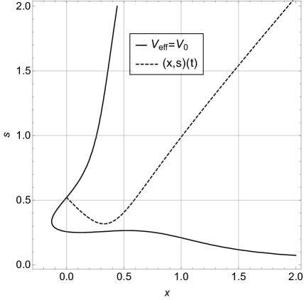
Figure 1: Dynamics in the all-orders effective potential (187): The potential is represented by its ground-state equipotential curve $V_{\rm{eff}}=V_{0}$ (solid line), together with a tunneling trajectory starting from the local minimum (dashed line). For this plot we chose the parameters $V_{\rm top}=1$, $\gamma=0.1$, $U=1/4$. The “extra dimension” given by the fluctuation parameter $s$ provides the particle with an escape route around the classical barrier, without violating energy conservation.

Using the all-orders potential, we estimate the tunneling time as a function of the tunnel exit position of the particle, which corresponds to the particle position around the critical point $q_{\rm{top}}\approx 2/3$. Figures 2 and 3 show numerical comparison of the canonical tunneling time and the exit momentum of the particle, using the all-orders potential and exact solutions, respectively.

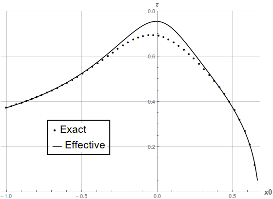
Figure 2: Tunneling times as a function of the starting position, for an exact calculation and the all-orders potential, respectively. There is good agreement, with larger discrepancies close to the origin where we have deep tunneling.

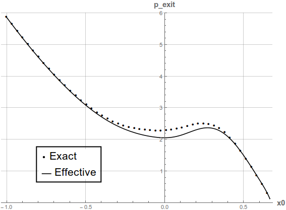
Figure 3: The exit momentum of the particle as a function of the initial position.

In [4] we used the all-orders effective potential for atomic systems, based on the all-orders closure condition. In a further approximation, it was possible to eliminate some of the basic variables such that $s\approx q$ inside the barrier. For the polynomial potential we can test the same behavior by computing the evolution of the expectation value $q$ and its fluctuation $s$. As shown Fig. 4, the approximate relationship between $q$ and $s$ during tunneling is maintained also here.

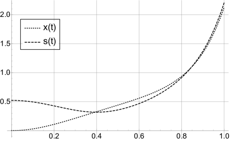
Figure 4: Trajectories of the tunneling coordinate $q$ and its fluctuation $s$ for the all-orders effective potential (187).

Finally, it is interesting to note that the tunneling time can be sensitive to the parameter $\gamma$ which specifies the location of the global minimum of the classical potential (184). We estimate the tunneling time in terms of $\gamma$, starting with $\gamma=0.1$, as shown in Fig. 5.

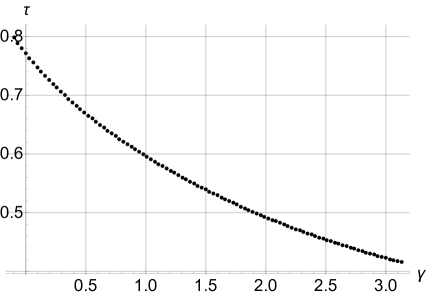
Figure 5: The tunneling time as a function of $\gamma$ in the potential (184).

3.3 Effective potentials

Casimir–Darboux coordinates for moments, in combination with the effective Hamiltonian (2), allow us to identify the dynamics of a semiclassical truncation with a dynamical canonical system. The classical momentum $\pi$ (derived from the momentum expectation value) is then accompanied by one or more new momenta that parameterize fluctuations, correlations, and higher moments.

For a single classical pair of degrees of freedom to second semiclassical order, the moments are quadratic in the new momentum $p_{s}$ with constant coefficients. A dynamical system with standard kinetic term is therefore obtained [9]:

$$\langle\hat{H}\rangle = \frac{\langle\hat{\pi}^{2}\rangle}{2m}+V(\hat{q})=\frac{\pi^{2}+\Delta(\pi^{2})}{2m}+V(q)+\frac{1}{2}V^{\prime\prime}(q)\Delta(q^{2})+\cdots$$ (192)

$$= \frac{\pi^{2}}{2m}+\frac{p_{s}^{2}}{2m}+\frac{U}{2ms^{2}}+V(q)+\frac{1}{2}V^{\prime\prime}(q)s^{2}+\cdots$$

with effective potential

$$V_{\rm eff}(q,s)=\frac{U}{2ms^{2}}+V(q)+\frac{1}{2}V^{\prime\prime}(q)s^{2}\,.$$ (193)

Our third-order moments provide an extension to the next order, now with three non-classical momenta. The first version, (61), is quadratic in momenta but with coefficients depending on the configuration variables $s_{i}$. The second version, (71), results in a simplified system with constant coefficients in the extended kinetic term.

However, for two pairs of degrees of freedom, it is not possible to have momentum fluctuations which are quadratic in Darboux momenta with constant coefficients [3]. The resulting effective theories are therefore more involved in such cases. Nevertheless, it is possible to extract an effective potential. Using the Taylor expansion (2) of the effective Hamiltonian $\langle\hat{H}\rangle$ and setting all canonical momenta equal to zero, we obtain an expression depending only on the canonical coordinates. We do not require that the momenta vanish for all solutions of interest, which would then be adiabatic, but rather extract a term from the effective Hamiltonian that serves as an effective potential. For this purpose, canonical variables are required in order to know which functions of the moments should be considered momenta.

For two classical degrees of freedom to second semiclassical order, this procedure leads to the effective potential

$$V^{(1)}_{\mathrm{eff}}(q_{1},q_{2},s_{1},s_{2},\alpha,\beta,U_{1},U_{2}) = V(q_{1},q_{2})$$

$$+\frac{1}{4\sin^{2}(\beta)}\left(\frac{U_{1}-\sqrt{U_{2}}\sin(\alpha+\beta)}{s_{1}^{2}}+\frac{U_{1}-\sqrt{U_{2}}\sin(\alpha-\beta)}{s_{2}^{2}}\right)$$

$$+\frac{1}{2}V_{11}(q_{1},q_{2})s_{1}^{2}+V_{12}(q_{1},q_{2})s_{1}s_{2}\cos{\left(\beta\right)}+\frac{1}{2}V_{22}(q_{1},q_{2})s_{2}^{2}$$

We have used the notation $V_{ij}=\partial^{2}V/\partial q_{i}\partial q_{j}$, and $V(q_{1},q_{2})$ is the classical potential. The two Casimir coordinates $U_{1}$ and $U_{2}$ are constants of motion for any classical dynamics and can be considered (state-dependent) parameters of the effective potential, while the remainder in the effective Hamiltonian is a non-standard kinetic term.

We define the low-energy effective potential $V_{\rm low}(q_{1},q_{2})$ as the effective potential $V_{\rm eff}$ restricted to values of the moments (that is, $s_{1}$, $s_{2}$, $\alpha$, $\beta$, $U_{1}$ and $U_{2}$) obtained in the ground state of the interaction system. We therefore determine the moments by minimizing the effective potential with respect to $s_{1}$, $s_{2}$, $\alpha$, $\beta$ and the two Casimir coordinates while keeping the classical-type variables $q_{1}$ and $q_{2}$ free.

In this process, we have to respect the boundaries imposed by uncertainty relations. Since $W$ is linear in $U_{1}$ and $\sqrt{U_{2}}$, minimization sends these two values to the boundary. (From (135), we know that $U_{2}>0$ for $p_{4}=0$ to be possible.) The relevant boundary components, at zero momenta, can be obtained from Heisenberg’s uncertainty relation applied to each canonical pair:

$$\Phi(\beta,0,\alpha,0) = \frac{1}{2\sin{(\beta)}^{2}}\left(U_{1}-\sqrt{U_{2}}\sin{(\alpha+\beta)}\right)\geq\frac{\hbar^{2}}{4}$$ (195)

$$\Gamma(\beta,0,\alpha,0) = \frac{1}{2\sin{(\beta)}^{2}}\left(U_{1}-\sqrt{U_{2}}\sin{(\alpha-\beta)}\right)\geq\frac{\hbar^{2}}{4}\,.$$ (196)

For fixed $U_{1}$ and $U_{2}$, these two relations must be true for all $\alpha$ and $\beta$. Moreover, for any choice of $U_{1}$ and $U_{2}$ there must be solutions of $\alpha$ and $\beta$ such that both relations are saturated: If the coupling between the two degrees of freedom is turned off adiabatically we expect saturation in the ground state. Since $U_{1}$ and $U_{2}$ are constants of motion for any Hamiltonian, their values do not change during this adiabatic decoupling. Therefore, any choice of $U_{1}$ and $U_{2}$ must allow some solutions of $\alpha$ and $\beta$ such that the uncertainty relations are saturated.

At saturation, we can subtract (195) and (196) and obtain

$$-\frac{1}{2}\sqrt{U_{2}}\frac{\cos(\alpha)}{\sin(\beta)}=0\,,$$ (197)

and thus $U_{2}=0$ or $\cos(\alpha)=0$. In the latter case, the $U_{2}$-dependent term in the effective potential,

$$V_{U_{2}}=-\frac{\sqrt{U_{2}}\cos(\beta)}{4\sin^{2}(\beta)}\left(\frac{1}{s_{1}^{2}}+\frac{1}{s_{2}^{2}}\right)\,,$$ (198)

is, for any classical potential, unbounded from below in $\sqrt{U_{2}}$ for any $\beta$ such that $\cos(\beta)>0$. This solution of (197) is therefore ruled out by the condition that a stable ground state must exist for a large class of classical potentials. We conclude that $U_{2}=0$.

Given this solution, the smallest value of $U_{1}$ for which (195) can be fulfilled is $U_{1}=\hbar^{2}/2$. Therefore,

$$\Phi|_{p_{3}=p_{4}=U_{2}=0,U_{1}=\hbar^{2}/2}=\frac{\hbar^{2}}{4\sin{\beta}^{2}}=\Gamma_{p_{3}=p_{4}=U_{2}=0,U_{1}=\hbar^{2}/2}$$ (199)

from (2.3.5) and (2.3.5). The effective potential then reads

$$V^{(2)}_{\mathrm{eff}}(q_{1},q_{2},s_{1},s_{2},\beta) = V(q_{1},q_{2})$$ (200)

$$+\frac{\hbar^{2}}{8\sin{(\beta)}^{2}s_{1}^{2}}+\frac{\hbar^{2}}{8\sin{(\beta)}^{2}s_{2}^{2}}+\frac{1}{2}V_{11}s_{1}^{2}$$

$$+V_{12}s_{1}s_{2}\cos{\left(\beta\right)}+\frac{1}{2}V_{22}s_{2}^{2}\,.$$

Although we have not minimized the potential in the direction of $\alpha$, the $\alpha$-dependence has disappeared. There should, however, be a unique pure state that corresponds to the ground state where the effective potential has its minimum. Since minimization does not determine $\alpha$, it must be the pure-state condition that fixes its value. This conclusion is in agreement with our earlier discussion of impurity parameters: In the mapping (149)–(156), $\alpha$ appears only in moments of the form $\Delta(\pi_{i}\pi_{j})$ which are not required to reconstruct a pure state in the position representation.

Minimization by $s_{1}$, $s_{2}$ and $\beta$ gives us three equations:

$$0 = \frac{\partial V^{(2)}_{\rm eff}}{\partial s_{1}}=-\frac{\hbar^{2}}{4s_{1}^{3}\sin^{2}\beta}+V_{11}s_{1}+V_{12}s_{2}\cos\beta$$ (201)

$$0 = \frac{\partial V^{(2)}_{\rm eff}}{\partial s_{2}}=-\frac{\hbar^{2}}{4s_{2}^{3}\sin^{2}\beta}+V_{22}s_{2}+V_{12}s_{1}\cos\beta$$ (202)

$$0 = \frac{\partial V^{(2)}_{\rm eff}}{\partial\beta}=-\frac{\hbar^{2}(s_{1}^{2}+s_{2}^{2})\cos\beta}{4s_{1}^{2}s_{2}^{2}\sin^{2}\beta}-V_{12}s_{1}s_{2}\sin\beta\,.$$ (203)

Subtracting $s_{2}$ times (202) from $s_{1}$ times (201), we obtain

$$\sin^{2}\beta=\frac{\hbar^{2}}{4s_{1}^{2}s_{2}^{2}}\frac{s_{2}^{2}-s_{1}^{2}}{V_{11}s_{1}^{2}-V_{22}s_{2}^{2}}\,.$$ (204)

Using the sum of $s_{2}$ times (202) and $s_{1}$ times (201), we derive

$$4V_{12}^{2}s_{1}^{2}s_{2}^{2}\cos^{2}\beta = \left(\frac{\hbar^{2}(s_{1}^{2}+s_{2}^{2})}{4s_{1}^{2}s_{2}^{2}\sin^{2}\beta}-(V_{11}s_{1}^{2}+V_{22}s_{2}^{2})\right)^{2}$$ (205)

$$= \left(\frac{s_{1}^{2}+s_{2}^{2}}{s_{1}^{2}-s_{2}^{2}}(V_{11}s_{1}^{2}-V_{22}s_{2}^{2})+(V_{11}s_{1}^{2}+V_{22}s_{2}^{2})\right)^{2}$$ (206)

$$= 4\frac{(V_{11}s_{1}^{4}-V_{22}s_{2}^{4})^{2}}{(s_{1}^{2}-s_{2}^{2})^{2}}\,.$$ (207)

Alternatively, we can derive $4V_{12}^{2}s_{1}^{2}s_{2}^{2}\cos^{2}\beta$ as follows: The sum of $s_{1}\sin^{2}\beta$ times (201) and $\cos\beta\sin\beta$ times (203) implies

$$0 = -\frac{\hbar^{2}(s_{1}^{2}+s_{2}^{2})}{4s_{1}^{2}s_{2}^{2}\sin^{2}\beta}+\frac{\hbar^{2}}{4s_{2}^{2}}+V_{11}s_{1}^{2}\sin^{2}\beta$$ (208)

$$= \frac{s_{1}^{2}+s_{2}^{2}}{s_{1}^{2}-s_{2}^{2}}(V_{11}s_{1}^{2}-V_{22}s_{2}^{2})+\frac{\hbar^{2}}{4}\frac{V_{11}-V_{22}}{V_{11}s_{1}^{2}-V_{22}s_{2}^{2}}$$ (209)

using (204). This equation together with (204) also gives us

$$4V_{12}^{2}s_{1}^{2}s_{2}^{2}\cos^{2}\beta = 4V_{12}^{2}s_{1}^{2}s_{2}^{2}\left(1-\frac{2\hbar^{2}}{s_{1}^{2}s_{2}^{2}}\frac{s_{2}^{2}-s_{1}^{2}}{V_{11}s_{1}^{2}-V_{22}s_{2}^{2}}\right)$$ (210)

$$= 4V_{12}^{2}\left(s_{1}^{2}s_{2}^{2}+(s_{1}^{2}+s_{2}^{2})\frac{V_{11}s_{1}^{2}-V_{22}s_{2}^{2}}{V_{11}-V_{22}}\right)$$ (211)

$$= 4V_{12}^{2}\frac{V_{11}s_{1}^{4}-V_{22}s_{2}^{4}}{V_{22}-V_{11}}\,.$$ (212)

Equating (205) and (210), we have

$$V_{11}s_{1}^{4}-V_{22}s_{2}^{4}=\frac{V_{12}^{2}}{V_{22}-V_{11}}(s_{1}^{2}-s_{2}^{2})^{2}$$ (213)

which can be interpreted as a quadratic equation for $s_{1}^{2}/s_{2}^{2}$ with solution

$$\frac{s_{1}^{2}}{s_{2}^{2}}=\frac{(V_{22}-V_{11})\sqrt{V_{11}V_{22}-V_{12}^{2}}-V_{12}^{2}}{V_{11}(V_{22}-V_{11})-V_{12}^{2}}\,.$$ (214)

(There is a unique sign choice implied by $s_{1}^{2}/s_{2}^{2}>0$.)

This solution implies

$$\frac{s_{1}^{2}+s_{2}^{2}}{s_{1}^{2}-s_{2}^{2}} = \frac{(V_{22}-V_{11})\left(\sqrt{V_{11}V_{22}-V_{12}^{2}}+V_{11}\right)-2V_{12}^{2}}{(V_{22}-V_{11})\left(\sqrt{V_{11}V_{22}-V_{12}^{2}}-V_{11}\right)}$$ (215)

$$V_{11}\frac{s_{1}^{2}}{s_{2}^{2}}-V_{22} = (V_{22}-V_{11})\sqrt{V_{11}V_{22}-V_{12}^{2}}\frac{V_{11}-\sqrt{V_{11}V_{22}-V_{12}^{2}}}{V_{11}(V_{22}-V_{11})-V_{12}^{2}}$$ (216)

which can be used in (208) to obtain

$$s_{2}^{4}=\frac{\hbar^{2}}{4}\frac{V_{11}V_{22}-V_{12}^{2}-V_{11}^{2}}{V_{11}V_{22}-V_{12}^{2}}\frac{V_{11}+\sqrt{V_{11}V_{22}-V_{12}^{2}}}{(V_{22}-V_{11})\sqrt{V_{11}V_{22}-V_{12}^{2}}+V_{11}V_{22}-V_{11}^{2}-2V_{12}^{2}}\,.$$ (217)

We also have

$$s_{1}^{4} = s_{2}^{4}(V_{11}\leftrightarrow V_{22})$$ (218)

$$= \frac{\hbar^{2}}{4}\frac{V_{11}V_{22}-V_{12}^{2}-V_{22}^{2}}{V_{11}V_{22}-V_{12}^{2}}\frac{V_{22}+\sqrt{V_{11}V_{22}-V_{12}^{2}}}{(V_{11}-V_{22})\sqrt{V_{11}V_{22}-V_{12}^{2}}+V_{11}V_{22}-V_{22}^{2}-2V_{12}^{2}}\,,$$ (219)

and the angle $\beta$ can be obtained by (204).

If we insert these solutions in the effective potential, the results can be seen to equal the low-energy effective potential [11]

$$V_{\mathrm{low}}(q_{1},q_{2}) = V(q_{1},q_{2})+\frac{\hbar}{2}\sqrt{\frac{1}{2}\left(V_{11}+V_{22}+\sqrt{\left(V_{11}-V_{22}\right)^{2}+4V_{12}^{2}}\right)}$$ (221)

$$+\frac{\hbar}{2}\sqrt{\frac{1}{2}\left(V_{11}+V_{22}-\sqrt{\left(V_{11}-V_{22}\right)^{2}+4V_{12}^{2}}\right)}\,.$$

although it initially appears in a rather different algebraic form. Our derivation automatically provides results for the ground-state variances and covariance at the minimum of the effective potential. For instance, while the actual expression for $\beta$ is quite complicated and not given here, for small $V_{12}$ we can use a Taylor expansion and obtain

$$\beta=\frac{\pi}{2}+\frac{V_{12}}{(V_{11}V_{22})^{1/4}\left(\sqrt{V_{11}}+\sqrt{V_{22}}\right)}+O(V_{12}^{2})\,.$$ (222)

In the limit of weak coupling, the moment $\Delta(q_{1}q_{2})$ therefore goes to zero.

As a simple example, consider the Hamiltonian

$$H=\frac{1}{2}\pi_{1}^{2}+\frac{1}{2}\pi_{2}^{2}+\frac{\omega^{2}}{2}q_{1}^{2}+\frac{\omega^{2}}{2}q_{2}^{2}+\gamma\omega^{2}q_{1}q_{2}\,.$$ (223)

Its quantization has the exact ground-state energy

$$E=\frac{1}{2}\hbar\omega\left(\sqrt{1+\gamma}+\sqrt{1-\gamma}\right)$$ (224)

agreeing with what we get from (221).

4 Discussion

Our extensions of canonical variables for moments from second order for a single degree of freedom demonstrate several new features of semiclassical states and their dynamics. In particular, we have identified various parameters related to the impurity of a state, a result which also plays a role in the determination of semiclassical potentials. Canonical moment variables are therefore useful tools to understand features of the quantum state space.

Our other applications illustrate the fact that canonical mappings of the form derived here can be relevant in a large set of different physical fields. For instance, they allow one to rewrite quantum statistics in classical terms and thereby provide convenient access to new types of variables (Section 3.1). Interestingly, there is a well-defined partition function for second-order moments even though these variables are subject to a non-invertible Poisson structure. For a derivation of the correct phase-space volume element it is therefore crucial to identify Casimir–Darboux variables. Casimir variables do not have momenta and therefore do not contribute the usual $2\pi\hbar$-volume to a partition function. Nevertheless, in our example we saw that we have to integrate over them in order to obtain the correct thermodynamical results for fluctuations.

In tunneling situations, canonical moment variables demonstrate a new heuristic picture of tunneling in which an external field literally opens up a tunnel through a higher-dimensional extension of the classical potential (Fig. 1). During tunneling, higher than second-order moments are crucial, which we have captured by the new all-orders effective potential (176) defined here for any classical potential. A separate paper [4] provides a detailed application to tunneling ionization in atoms with a successful comparison with recent discussions of experimental results, for which the closure conditions discussed here provide the foundation.

References

- [1] M. Bojowald and A. Skirzewski, Effective Equations of Motion for Quantum Systems, Rev. Math. Phys. 18 (2006) 713–745, [math-ph/0511043]
- [2] M. Bojowald and A. Skirzewski, Quantum Gravity and Higher Curvature Actions, Int. J. Geom. Meth. Mod. Phys. 4 (2007) 25–52, [hep-th/0606232]
- [3] B. Baytaş, M. Bojowald, and S. Crowe, Faithful realizations of semiclassical truncations, [arXiv:1810.12127]
- [4] B. Baytaş, M. Bojowald, and S. Crowe, Canonical Tunneling Time in Ionization Experiments, [arXiv:1810.12804]
- [5] A. Tsobanjan, Semiclassical states on Lie algebras, J. Math. Phys. 56 (2015) 033501, [arXiv:1410.0704]
- [6] M. Bojowald, D. Brizuela, H. H. Hernandez, M. J. Koop, and H. A. Morales-Técotl, High-order quantum back-reaction and quantum cosmology with a positive cosmological constant, Phys. Rev. D 84 (2011) 043514, [arXiv:1011.3022]
- [7] V. I. Arnold, Mathematical Methods of Classical Mechanics, Springer, 1997
- [8] F. Arickx, J. Broeckhove, W. Coene, and P. van Leuven, Gaussian Wave-packet Dynamics, Int. J. Quant. Chem.: Quant. Chem. Symp. 20 (1986) 471–481
- [9] O. Prezhdo, Quantized Hamiltonian Dynamics, Theor. Chem. Acc. 116 (2006) 206
- [10] C. Kühn, Moment Closure—A Brief Review, In Control of Self Organizing Non-Linear Systems, pages 253–271, Springer International Publishing, 2016
- [11] F. Cametti, G. Jona-Lasinio, C. Presilla, and F. Toninelli, Comparison between quantum and classical dynamics in the effective action formalism, In Proceedings of the International School of Physics “Enrico Fermi”, Course CXLIII, pages 431–448, Amsterdam, 2000. IOS Press, [quant-ph/9910065]