Modeling Attention Flow on Graphs

Abstract

Real-world scenarios demand reasoning about process, more than final outcome prediction, to discover latent causal chains and better understand complex systems. It requires the learning algorithms to offer both accurate predictions and clear interpretations. We design a set of trajectory reasoning tasks on graphs with only the source and the destination observed. We present the attention flow mechanism to explicitly model the reasoning process, leveraging the relational inductive biases by basing our models on graph networks. We study the way attention flow can effectively act on the underlying information flow implemented by message passing. Experiments demonstrate that the attention flow driven by and interacting with graph networks can provide higher accuracy in prediction and better interpretation for trajectory reasoning.

1 Introduction

Many practical applications have the need to infer latent causal chains or to construct interpretations for observations or some predicted results. For example, in a physical world, we want to reason the trajectories of moving objects given very few observed frames; in a video streaming system, we wish recommendation models that track the evolving user interests to provide personalized recommendation reasons linking users’ watched videos to the recommended ones. Here, we focus on graph-based scenarios, and aim to infer latent chains that might cause observed results described by nodes and edges in a given graph.

Graph networks [1, 2, 3, 4, 5] are a family of neural networks that operate on graphs and carry strong relational inductive biases. It is believed that graph networks have a powerful fitting capacity to deal with graph-structured data. However, its black-box nature makes it less competitive than other differentiable logic-based reasoning [6, 7, 8] when modeling the reasoning process with interpretations provided. In this work, we develop a new attention mechanism on graphs, called attention flow, to model the reasoning process to predict the final outcome with the interpretability. We use the message passing algorithm in graph networks to derive a transition matrix evolving with time steps to drive the attention flow. We also let the attention flow act back on the passed messages, called information flow. To evaluate the models, we design a set of trajectory reasoning tasks, where only the source and destination ends of trajectories are observed.

Our contributions are two-fold. First, our attention flow mechanism, built on graph networks, introduces a new way to construct interpretations and increase the transparency when applying graph networks. Second, we show how attention flow can effectively intervene back in message passing conducted in graph networks, analogous to that of reinforcement learning where actions taken by agents would affect states of the environment. Experiments demonstrate that the graph network models with the explicit and backward-acting attention flow compare favorably both in prediction accuracy and in interpretability against those without it.

Related Works. Graph networks[3, 4, 5], dating back to a decade ago [1, 2], are thought to support relational reasoning and combinatorial generalization over graph-structured representations. Recently, this area has grown rapidly and many versions of graph networks have been proposed, including Gated Graph Neural Networks [9], Interaction Networks [10], Relation Networks [11], Message Passing Neural Networks [12], Graph Attention Networks [13], Non-Local Neural Networks [14], and the graph convolutional network family [15], spectral [16, 17, 18, 19] or non-spectral [20, 21, 22, 23, 24]. From a unified perspective, [12] introduces the message passing mechanism to generalize computation frameworks on graphs; [3] uses the term of graph networks to generalize and extend several lines in this area. While graph networks give reasoning over graphs more fitting capacity, we look back on the old-fashioned logic and rules-based reasoning to seek the interpretability. Recent probabilistic logic programming, such as TensorLog [6, 7] and NeuralLP [8], develops differentiable reasoning based on a knowledge graph, learning soft logic rules in an end-to-end style, and the process is much like a rooted random walk computing conditional probabilities based on paths. People also studied reasoning over paths or graphs using reinforcement learning to deal with discrete actions of choosing nodes or edges, such as MINERVA [25], Structure2Vec Deep Q-learning [26], and Neural Combinatorial Optimization [27]. Attention mechanisms, derived from sequence-based tasks [28], developed in [29] referred to as self-attention, have been brought in graphs recently by attending over neighbors of each node [13, 30] or non-local areas [14]. Here, we present the attention flow mechanism not only for the computation need but also for the interpretation purpose.

2 Tasks

Real-world scenarios often demand reasoning about process, that is, constructing interpretations by listing a series of causal connections linking an opening to an outcome. We need a simulation system to generate a trajectory of events with the dynamics governed by latent factors, such as the trajectory of a moving object controlled by an external force. Instead of full observation, we only allow events at the source and the destination observed, treating the task as a trajectory reasoning problem.

We build a corrupted $N\times N$ grid world with a small fraction of nodes or edges randomly removed. There are 8 types of directed edges at most for each node, connecting it to its neighbors, such as east (E) and northeast (NE). Picking an arbitrary node as the source $v^{0}$, we draw a sequence of consecutive nodes to construct a trajectory $(v^{0},v^{1},\ldots,v^{T})$ and obtain the final node $v^{T}$ as the destination. Each node on the trajectory except the source is chosen from the neighborhood of the previous node $v_{x,y}$ by drawing one of the 8 edge types $e$ from the distribution below driven by latent direction function $\vec{d}_{t,x,y}$ varying with time $t$ and location $(x,y)$:

$$\begin{split}&P(e)\propto\exp{\Big{(}\big{\langle}\vec{d}_{e}/\|\vec{d}_{e}\|,\vec{d}_{t,x,y}/\|\vec{d}_{t,x,y}\|\big{\rangle}/\sigma^{2}\Big{)}},\quad e\in\{E,NE,N,NW,W,SW,S,SE\}\\ &\vec{d}_{t,x,y}=(a_{1}\cos{\theta_{t,x,y}}+b_{1},a_{2}\sin{\theta_{t,x,y}}+b_{2}),\quad\theta_{t,x,y}=\omega t+\lambda_{1}x+\lambda_{2}y+\phi\end{split}$$ (1)

The trajectory terminates by either choosing a non-existent edge or reaching the maximal steps. To be specific, we generate four types of trajectories governed by:

• $\vec{d}_{t,x,y}=(1,0.4)$, a straight line with a slope.

• $\vec{d}_{t,x,y}=(1,\sin(0.4t+1.6))$, a sine curve with directions varying with time $t$.

• $\vec{d}_{t,x,y}=(\cos\theta_{x,y},\sin\theta_{x,y})$, $\theta_{x,y}=0.2x+0.2y$, directions varying with the current location.

• $\vec{d}_{t,x,y}=(\cos\theta_{x,y},\sin\theta_{x,y})$, $\theta_{x,y}=0.2\max{\{x_{i}\}}+0.2\max{\{y_{i}\}}$, depending on location history.

Instead of learning a latent model to solve the trajectory reasoning problem, we use a supervised setting. Considering only the source and the destination available, we train a discriminative model to predict the destination node by inputting the source node. We leverage the graph structure in the corrupted grid world, as the problem implies strong inductive biases on graphs, relational (sequences of consecutive nodes) and non-relational (latent direction functions depending on time, location and history). The trajectory reasoning problem is difficult considering that many candidate paths link the source to the destination. The only clue we can observe is the destination nodes resulting from the blocked trajectories caused by removed nodes or edges. Note that we do not look for the shortest paths but the true trajectory pattern governed by some latent dynamics. The evaluation criteria should be based on both the accuracy of prediction and the human readability of interpretation.

3 Models

Modeling attention flow on graphs. We view the problem of predicting the destination given the source as predicting the output attention distribution over nodes given the input attention distribution. We use the term of attention distribution to represent the probability distribution of attending over nodes. For each pair $(v_{src},v_{dst})$, the input attention distribution has all the probability mass concentrated on the source node. After a series of computation on the graph, the resulting output attention distribution predicts the most likely node to be the destination. Attention transfers from the source to the destination, implying a flow through the graph mimicking latent causal chains. The followings attempt to model the attention flow on graphs from three different perspectives.

Implicit attention flow in graph networks. Modern graph networks (GNs) mostly employ the message passing mechanism implemented by neural network building blocks, such as MLP and GRU modules. Representations in GNs include node-level states $\mathbf{h}_{i}\in\mathbb{R}^{d}$, edge-level messages $\mathbf{m}_{ij}\in\mathbb{R}^{d}$ and sometimes graph-level global state $\mathbf{g}\in\mathbb{R}^{d}$. A GN framework has three phases: the initialization phase, the propagation phase, and the output phase. The model in the propagation phase includes:

• Message function: $\mathbf{m}^{t}_{ij}=f_{\mathrm{msg}}(\mathbf{h}^{t}_{i},\mathbf{h}^{t}_{j},\mathbf{g}^{t};\theta_{e_{ij}})$, where $\theta_{e_{ij}}$ is edge type-specific parameters.

• Message aggregation operation: $\mathbf{\bar{m}}^{t}_{j}=\sum_{i}\mathbf{m}^{t}_{ij}$, aggregating all received messages from neighbors.

• Node update function: $\mathbf{h}^{t+1}_{i}=f_{\mathrm{node}}(\mathbf{h}^{t}_{i},\mathbf{\bar{m}}^{t}_{i},\mathbf{g}^{t},\mathbf{u}_{i})$, where $\mathbf{u}_{i}$ is stationary node embeddings.

• Global update function: $\mathbf{g}^{t+1}=f_{\mathrm{global}}(\mathbf{g}^{t},\mathbf{\bar{h}}^{t},\mathbf{\bar{m}}^{t})$, where $\mathbf{\bar{h}}^{t}=\frac{1}{|\mathcal{V}|}\sum_{i}\mathbf{h}^{t}_{i},\;\mathbf{\bar{m}}^{t}=\frac{1}{|\mathcal{V}|}\sum_{i}\mathbf{\bar{m}}^{t}_{i}$.

To model the attention flow, we modify the initialization phase by defining $\mathbf{h}^{0}_{i}:=[\mathbf{\dot{h}}^{0}_{i}:\mathbf{\ddot{h}}^{0}_{i}]$ where $\mathbf{\dot{h}}^{0}_{i}\in\mathbb{R}^{d^{\prime}}$ is attention channels and $\mathbf{\ddot{h}}^{0}_{i}\in\mathbb{R}^{d-d^{\prime}}$ auxiliary channels. We initialize $\mathbf{\dot{h}}^{0}_{\mathrm{src}}=\mathbf{\tilde{1}}$ for the source and $\mathbf{\dot{h}}^{0}_{i}=\mathbf{0}$ for the rest where $\mathbf{\tilde{1}}:=\mathbf{1}/\|\mathbf{1}\|$ acts as a reference vector for computing attention distributions, so that score $\langle\mathbf{\dot{h}}^{0}_{i},\mathbf{\tilde{1}}\rangle$ is $1$ on the source node and $0$ on the rest. We set $\mathbf{\ddot{h}}^{0}_{i}=f_{\mathrm{init}}(\mathbf{u}_{i})$. At the output phase, we compute the output attention distribution by $\mathrm{softmax}({\langle\mathbf{\dot{h}}^{T}_{i},\mathbf{\tilde{1}}\rangle}_{i=1}^{n})$.

This model wraps the attention flow in the messages passing process at the beginning and takes it out at the end. Neural network-based computation makes the propagation model a black box, lacking an explicit way to depict the attention flow, helpless for the interpretation purpose.

Explicit attention flow by random walks. To explicitly model the attention flow, we use random walks with learnable transition $\mathbf{T}$. The dynamics of attention flow are driven by $\mathbf{a}^{t+1}=\mathbf{T}\mathbf{a}^{t}$ where $\mathbf{a}^{t+1}$ and $\mathbf{a}^{t}$ represent two consecutive attention distributions. Here, we take two model settings:

• Stationary transition setting: $\tau_{ij}=f_{\mathrm{trans}}(\mathbf{u}_{i},\mathbf{u}_{j};\phi_{e_{ij}})$ and do the row-level softmax to get entry $T_{ij}$. The transition $\mathbf{T}$ is stationary across inputs and steps.

• Dynamic transition setting: $\tau^{t}_{ij}=f_{\mathrm{trans}}(\mathbf{h}^{t}_{i},\mathbf{h}^{t}_{j};\phi_{e_{ij}})$ where $\mathbf{h}^{t+1}_{i}=f_{\mathrm{node}}(\mathbf{h}^{t}_{i},\mathbf{g}^{t},\mathbf{u}_{i})$, $\mathbf{g}^{t+1}=f_{\mathrm{global}}(\mathbf{g}^{t},\mathbf{\bar{h}}^{t})$ and $\mathbf{\bar{h}}^{t}=\sum_{i}a^{t}_{i}\mathbf{h}^{t}_{i}$. Note that no message passing is applied. The update on global state $\mathbf{g}^{t}$ is based on the weighted sum of node states affected by $\mathbf{a}^{t}$. We emphasize that attention distributions can act as more than output of internal states and effectively impact back on the internal. The graph context captured this way is still limited without leveraging message passing.

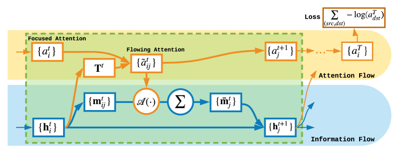
Figure 1: The two-flow model architecture.

Explicit attention flow with graph networks. The interpretability benefit of explicit attention flow can be gained even when enjoying the expressivity of graph networks. We present the attention flow mechanism by introducing the node-level attention, called focused attention $\mathbf{a}$, and the edge-level attention, called flowing attention $\mathbf{\tilde{a}}$. With the superscript step $t$, the dynamics are driven by:

$$\tilde{a}^{t}_{ij}=T^{t}_{ij}a^{t}_{i},\quad a^{t+1}_{j}=\sum_{i}\tilde{a}^{t}_{ij},\quad\mathrm{s.t.}\sum_{i}a^{t}_{i}=1,\quad\sum_{ij}\tilde{a}^{t}_{ij}=1,$$ (2)

where transition $\mathbf{T}^{t}$ relies on the rich context carried by the underlying message passing in GNs, thus called information flow, in addition to attention flow. See the two-flow model architecture in Figure 1.

It is obvious that the information flow determines the attention flow, but we are more curious about how the attention flow can affect back the information flow. We have seen the node-level backward acting of the focused attention on the sum of node states as above. Here, we study on the edge level how the flowing attention acts on the information flow by defining the message-attending function $\mathbf{\tilde{m}}^{t}_{ij}=\mathcal{A}(\tilde{a}^{t}_{ij},\mathbf{m}^{t}_{ij})$ to produce attended message $\mathbf{\tilde{m}}^{t}_{ij}$ to replace original message $\mathbf{m}^{t}_{ij}$:

• No acting: $\mathcal{A}(\tilde{a}^{t}_{ij},\mathbf{m}^{t}_{ij}):=\mathbf{m}^{t}_{ij}$

• Multiplying: $\mathcal{A}(\tilde{a}^{t}_{ij},\mathbf{m}^{t}_{ij}):=\tilde{a}^{t}_{ij}\cdot\mathbf{m}^{t}_{ij}$

• Non-linear acting after multiplying: $\mathcal{A}(\tilde{a}^{t}_{ij},\mathbf{m}^{t}_{ij}):=\mathrm{MLP}(\tilde{a}^{t}_{ij}\cdot\mathbf{m}^{t}_{ij})$

To design a meaningful $\mathcal{A}(\tilde{a}^{t}_{ij},\mathbf{m}^{t}_{ij})$, when $\tilde{a}^{t}_{ij}=0$ we make $\mathcal{A}(0,\mathbf{m}^{t}_{ij})$ independent from $\mathbf{m}^{t}_{ij}$, implying no attention paid to this piece of message but not necessarily being $0$. We find $\mathrm{MLP}(\tilde{a}^{t}_{ij}\cdot\mathbf{m}^{t}_{ij})$ performs the best in most cases, revealing not only the importance of backward acting but also the necessity of keeping information flow even if not being attended.

Connections to reinforcement learning and probabilistic latent models. If we inject noises and then pick the top-1 attended node each step, the process becomes similar to reinforcement learning in some way. If we apply noises but keep it soft in the Gumbel-Softmax [31] or Concrete [32] distribution, it turns into a probabilistic latent model. Attention flow can be viewed as graph-level computation operating directly andnumerically in a probability space rather than in a discrete sample space.

4 Experiments

4.1 Experimental Procedure

Dataset generation and statistics. We generate a number of dataset groups each representing a randomized grid world with a specific version of trajectories, consisting of sequences of nodes, driven by a specific setting of latent dynamics applied. More specifically, for each dataset group, we build a corrupted $N\times N$ grid world and then apply a latent direction function $\vec{d}_{t,x,y}$ to draw multiple trajectories starting from each node. The data generation parameters include:

• $N$: The size of a grid map. Without nodes and edges dropped, we have $N^{2}$ nodes and $2(2N-1)(2N-2)$ directed edges at most, where each internal node is connected to 8 incoming edges as well as 8 outgoing edges. In the experiments, we test models in two sizes: $32\times 32$ and $64\times 64$.

• $p_{\mathrm{node\_drp}}$ and $p_{\mathrm{edge\_drp}}$: The dropping probabilities of randomly removing a node or an edge. If a node is removed, all its connected edges should be gone; if a node is left with no edges, that is, a single isolated point, we remove it. When we remove an edge connected by a pair of nodes $v_{1}$ and $v_{2}$, we drop edges $(v_{1},v_{2})$ and $(v_{2},v_{1})$ in both directions. In the experiments, we try two settings: dropping nodes only with $p_{\mathrm{node\_drp}}=0.1$, and dropping edges only with $p_{\mathrm{edge\_drp}}=0.2$.

• $T$: The maximal steps of a trajectory. Without being blocked, a trajectory would end with a maximal length of $T$. In the experiments, we set $T=16$ in $32\times 32$ and $T=32$ in $64\times 64$. Therefore, the total problem scale depends on $N$, $p_{\mathrm{node\_drp}}$ and $p_{\mathrm{edge\_drp}}$, and $T$.

• $\sigma$: The standard deviation of sampling an edge around latent direction $\vec{d}_{t,x,y}$. Larger $\sigma$ increases the chance to bypass gaps caused by removed nodes and edges, and also brings a larger deviation of positions of the destination nodes given the same source, leading to a larger exploring area and more uncertainty for prediction. In the experiments, we pick two values, $\sigma=0.2$ and $\sigma=0.5$.

• $n_{\mathrm{rollout}}$: The number of rollouts to draw a trajectory starting from a specific node. With each node as a source, we try $n_{\mathrm{rollout}}$ times and then remove the duplicated source-destination pairs. In the experiments, we use $n_{\mathrm{rollout}}=10$.

• $\vec{d}_{t,x,y}$: The latent direction function. In the experiments, we try four settings as shown in Section 2: (1) a straight line with a constant sloped direction; (2) a sine curve with time-dependent varying directions; (3) a curve with location-dependent varying directions; (4) a curve with location history-dependent varying directions.

• $seed$: The datasets in each group share the same generation parameters listed above except $seed$. The purpose is to make experimental results less impacted by accidental factors. We use five random seeds in the experiments.

We generate $24$ dataset groups with their names and generation parameters listed in Table 4 in the appendix. Each dataset group contains five datasets with different $seed$s. The observed part of each dataset includes a grid map containing all edge information and a list of source-destination pairs used for training, validation and test. We make the training, validation and test sets by an $8:1:1$ splitting on source nodes, so that we can assess models based on their performances of handling pairs with unseen source nodes. The statistics of datasets are given in Table 5 in the appendix.

Models in comparison. To fully evaluate the attention flow mechanism, we choose three types of graph networks plus two random walk-based models to set the benchmark. Graph networks include a full Graph Network (FullGN) [3], a Gated Graph Neural Network (GGNN) [9], and a Graph Attention Network (GAT) [13]. Note that the regular versions of these graph networks are incapable to explicitly model attention flow and fulfill the trajectory reasoning purpose, though able to make predictions. We remodel them with the attention flow mechanism imposed respectively, which is implemented in three different ways on how the flowing attention acts back on the passed messages.

Regular graph networks. Node states $\mathbf{h}^{t}_{i}=[\mathbf{\dot{h}}^{t}_{i}:\mathbf{\ddot{h}}^{t}_{i}]\in\mathbb{R}^{d}$ have $d=40$ channels (or dimensions) where the number of attention channels is $d^{\prime}=8$ and the rest channels are left for carrying auxiliary messages. We tried several combinations for the pair of channel numbers and found 8 attention channels performed the best. To initialize $\mathbf{\dot{h}}^{0}_{i}$, we set $\mathbf{\dot{h}}^{0}_{src}=\mathbf{\tilde{1}}=\mathbf{1}/\sqrt{d^{\prime}}$ for the source node and $\mathbf{\dot{h}}^{0}_{i}=\mathbf{0}$ for the rest. We also initialize $\mathbf{\ddot{h}}^{0}_{i}=f_{\mathrm{init}}(\mathbf{u}_{i})$ where $\mathbf{u}_{i}\in\mathbb{R}^{d}$ represents stationary node embeddings and $f_{\mathrm{init}}$ is a single-layer feedforward network with the $\mathrm{tanh}$ activation function. The loss is defined in the cross entropy between the one-hot true destination labels and the predicted probability distribution by $\mathrm{softmax}({\langle\mathbf{\dot{h}}^{T}_{i},\mathbf{\tilde{1}}\rangle}_{i=1}^{n})$.

• FullGN: This model has global state $\mathbf{g}^{t}$, and both the message function and the node update function take $\mathbf{g}^{t}$ as one of their inputs. Here, each function uses a single-layer feedforward network.

  • Message function: $\mathbf{m}^{t}_{ij}=\tanh(\mathbf{W}_{e_{ij}}[\mathbf{h}^{t}_{i}:\mathbf{h}^{t}_{j}:\mathbf{g}^{t}]+\mathbf{b}_{e_{ij}})$.

  • Node update function: $\mathbf{h}^{t+1}_{i}=\tanh(\mathbf{W}_{\mathrm{node}}[\mathbf{h}^{t}_{i}:\mathbf{\bar{m}}^{t}_{i}:\mathbf{u}_{i}:\mathbf{g}^{t}]+\mathbf{b}_{\mathrm{node}})$.

  • Global update function: $\mathbf{g}^{t+1}=\tanh(\mathbf{W}_{\mathrm{global}}[\mathbf{g}^{t}:\mathbf{\bar{h}}^{t}:\mathbf{\bar{m}}^{t}]+\mathbf{b}_{\mathrm{global}})$.

• GGNN: This model computes messages in a non-pairwise linear manner that depends on sending nodes and edge types. It ignores the global state and changes the node update function into a gated recurrent unit (GRU).

  • Message function: $\mathbf{m}^{t}_{ij}=\mathbf{W}_{e_{ij}}\mathbf{h}^{t}_{i}+\mathbf{b}_{e_{ij}}$.

  • Node update function: $\mathbf{h}^{t+1}_{i}=\mathrm{GRU}(\mathbf{h}^{t}_{i},\;[\mathbf{\bar{m}}^{t}_{i}:\mathbf{u}_{i}])$.

• GAT: This model uses multi-head self-attention layers. Here, we take edge types into account to define weights. We also apply a GRU to the node update function, taking the concatenation of all multi-head aggregated messages $\mathbf{\bar{m}}_{i}^{t,k}$ and node embedding $\mathbf{u}_{i}$ as the input. We use $K=5$ heads each with an $8$-dimensional self-attention so that the concatenated message still has $40$ dimensions.

  • Multi-head self-attention: $\alpha^{t,k}_{ij}=\mathrm{softmax}_{j}(\mathrm{LeakyRelu}(\mathbf{a}^{T}[\mathbf{W}^{k}_{e_{i*}}\mathbf{h}^{t}_{i}:\mathbf{W}^{k}_{e_{i*}}\mathbf{h}^{t}_{*}]))$.

  • Message function: $\mathbf{m}^{t,k}_{ij}=\alpha^{t,k}_{ij}\mathbf{W}^{k}_{e_{ij}}\mathbf{h}^{t}_{i}$.

  • Node update function: $\mathbf{h}^{t+1}_{i}=\mathrm{GRU}(\mathbf{h}^{t}_{i},\;[\mathbf{\bar{m}}^{t,1}_{i}:\ldots:\mathbf{\bar{m}}^{t,K}_{i}:\mathbf{u}_{i}])$.

Remodeled graph networks with explicit attention flow. We add our attention flow module onto the computation framework of graph networks as shown in Figure 1. At the initialization phase, we define $\mathbf{a}^{0}$ by $a_{src}^{0}=1$ and $a_{i}^{0}=0$ for the rest; at the output phase, we take $\mathbf{a}^{T}$ to compute the loss:

$$\sum_{(src,dst)}-\log a_{dst}^{T}$$

For the propagation phase, we need to compute two more functions:

• Transition logits function: $\tau^{t}_{ij}=\mathbf{w}^{T}_{e_{ij}}[\mathbf{h}^{t}_{i}:\mathbf{h}^{t}_{j}:(\mathbf{h}^{t}_{i}\otimes\mathbf{h}^{t}_{j})]+b_{e_{ij}}$ in order to compute $\mathbf{T}^{t}$.

• Message-attending function: $\mathbf{\tilde{m}}^{t}_{ij}=\mathcal{A}(\tilde{a}^{t}_{ij},\mathbf{m}^{t}_{ij})$ to produce attended message $\mathbf{\tilde{m}}^{t}_{ij}$ in place of original message $\mathbf{m}^{t}_{ij}$. We study three ways to implement it: (1) no acting, (2) multiplying, (3) non-linear acting after multiplying. For (3), we simply use a single-layer feedforward network. Finally, we derive three explicit attention flow models based on each graph network.

  • {FullGN, GGNN, GAT}-NoAct.

  • {FullGN, GGNN, GAT}-Mul.

  • {FullGN, GGNN, GAT}-MulMlp.

Random walk-based models. If we model the attention flow without considering message passing conducted in graph networks, the method falls into the family of differentiable random walk models with a learned transition matrix. Here, we try two types of transition, stationary and dynamic.

• RW-Stationary:

  • Transition logits function: $\tau^{t}_{ij}=\mathbf{w}^{T}_{e_{ij}}[\mathbf{u}_{i}:\mathbf{u}_{j}:(\mathbf{u}_{i}\otimes\mathbf{u}_{j})]+b_{e_{ij}}$

• RW-Dynamic:

  • Transition logits function: $\tau^{t}_{ij}=\mathbf{w}^{T}_{e_{ij}}[\mathbf{h}^{t}_{i}:\mathbf{h}^{t}_{j}:(\mathbf{h}^{t}_{i}\otimes\mathbf{h}^{t}_{j})]+b_{e_{ij}}$.

  • Node update function: $\mathbf{h}^{t+1}_{i}=\tanh(\mathbf{W}_{\mathrm{node}}[\mathbf{h}^{t}_{i}:\mathbf{u}_{i}:\mathbf{g}^{t}]+\mathbf{b}_{\mathrm{node}})$.

  • Global update function: $\mathbf{g}^{t+1}=\tanh(\mathbf{W}_{\mathrm{global}}[\mathbf{g}^{t}:\mathbf{\bar{h}}^{t}]+\mathbf{b}_{\mathrm{global}})$ where $\mathbf{\bar{h}}^{t}=\sum_{i}a^{t}_{i}\mathbf{h}^{t}_{i}$.

Table 1: Comparison results on dataset groups {LINE,SINE,LOCATION,HISTORY}-SZ32-STP16-NDRP-STD0.2. This table focuses on comparative evaluation between all the explicit attention flow models that offer clear interpretations as well as prediction results, so that we gray the results from the implicit attention flow models, that is, regular graph networks. Each column indicates one comparison in a specific metric based on the same dataset group. $*$ represents the highest metric score acquired by random walk-based models. $\checkmark$ represents the graph network-based explicit attention flow models that beat the best random walk-based models. Futhermore, we compare the three message-attending approaches between the explicit attention flow models based on the same graph network, and then highlight the best in bold.

	LINE		SINE		LOCATION		HISTORY
Model	H@1(%)	MRR	H@1(%)	MRR	H@1(%)	MRR	H@1(%)	MRR
RW-Stationary	15.80	0.3409	8.56	0.2177	50.06$*$	0.6625$*$	16.44	0.3215
RW-Dynamic	16.64$*$	0.3562$*$	19.15$*$	0.3418$*$	45.94	0.6320	20.41$*$	0.3656$*$
FullGN	15.13	0.3451	51.71	0.6665	25.67	0.4393	16.61	0.3095
FullGN-NoAct	16.65$\checkmark$	0.3574$\checkmark$	30.10$\checkmark$	0.4476$\checkmark$	46.47	0.6337	20.80$\checkmark$	0.3729$\checkmark$
FullGN-Mul	16.69$\checkmark$	0.3636$\checkmark$	37.49$\checkmark$	0.4915$\checkmark$	43.44	0.6029	21.35$\checkmark$	0.3618
FullGN-MulMlp	16.99$\checkmark$	0.3662$\checkmark$	39.91$\checkmark$	0.5195$\checkmark$	50.93$\checkmark$	0.6598	23.94$\checkmark$	0.3850$\checkmark$
GGNN	15.49	0.3493	51.02	0.6611	29.20	0.4699	22.56	0.3677
GGNN-NoAct	16.64	0.3570$\checkmark$	25.14$\checkmark$	0.3918$\checkmark$	49.50	0.6621	21.69$\checkmark$	0.3818$\checkmark$
GGNN-Mul	16.95$\checkmark$	0.3610$\checkmark$	23.62$\checkmark$	0.3776$\checkmark$	45.22	0.6185	23.81$\checkmark$	0.3824$\checkmark$
GGNN-MulMlp	17.08$\checkmark$	0.3673$\checkmark$	34.75$\checkmark$	0.4699$\checkmark$	50.28$\checkmark$	0.6637$\checkmark$	26.06$\checkmark$	0.4001$\checkmark$
GAT	16.01	0.3469	43.19	0.5566	18.18	0.3583	12.11	0.2333
GAT-NoAct	16.02	0.3536	15.77	0.3221	46.10	0.6356	23.17$\checkmark$	0.3818$\checkmark$
GAT-Mul	15.86	0.3501	20.14$\checkmark$	0.3429$\checkmark$	45.83	0.6208	22.70$\checkmark$	0.3762$\checkmark$
GAT-MulMlp	17.07$\checkmark$	0.3646$\checkmark$	30.64$\checkmark$	0.4390$\checkmark$	47.52	0.6371	20.71$\checkmark$	0.3655

Training and evaluation details. Considering that trajectories might terminate before reaching the maximal steps, we add a selfloop edge onto each node so that we can treat all trajectories as ones with a fixed number of steps. Thus, there would be 9 types of edges during training. Our training hyperparameters include the batch size of $16$, the representation dimensions of $40$, the weight decay on node embeddings of $0.00001$, the decayed learning rates from $0.0005$ to $0.0001$ diminished by $0.0001$ every 10 epochs, and a total number of training epochs of $50$. We use the Adam SGD optimizer for all models. When dealing with larger datasets of $64\times 64$, we reduce the batch size to $4$ and the representation dimensions to $30$. During experiments, for each model we conducted 10 runs on each dataset group by five different generation seeds and two different input shufflings. We saved one model snapshot every epoch and chose the best three according to their validation performance, and then computed the mean and standard deviation of their evaluation metrics on the test set.

Evaluation metrics. We use Hits@1, Hits@5, Hits@10, the mean rank (MR), and the mean reciprocal rank (MRR) to evaluate these models. Hits@k means the proportion of test source-destination pairs for which the target destination is ranked in the top-k predictions, and thus Hits@1 is the prediction accuracy. Compared to Hits@k, MR and MRR can evaluate prediction results even when the target destination is ranked out of the top-k. MR provides a more intuitive sense about how many are ranked before the target on average, but often suffers from its instability susceptible to the worst example and becomes very large. MRR scores always range from $0.0$ to $1.0$. For MR lower score reflects better prediction, whereas for MRR higher score means better.

Table 2: Comparison results on dataset groups {LINE,SINE,LOCATION,HISTORY}-SZ32-STP16-NDRP-STD0.5. The marks in this table have the same meanings as Table 1.

	LINE		SINE		LOCATION		HISTORY
Model	H@1(%)	MRR	H@1(%)	MRR	H@1(%)	MRR	H@1(%)	MRR
RW-Stationary	15.74$*$	0.3348	9.07	0.2267	19.40$*$	0.3860$*$	11.72	0.2547
RW-Dynamic	15.48	0.3429$*$	13.38$*$	0.2905$*$	17.91	0.3722	12.25$*$	0.2820$*$
FullGN	14.61	0.3355	17.10	0.3525	16.09	0.3476	13.79	0.3051
FullGN-NoAct	15.50	0.3410	16.60$\checkmark$	0.3360$\checkmark$	18.83	0.3816	13.90$\checkmark$	0.3059$\checkmark$
FullGN-Mul	16.21$\checkmark$	0.3498$\checkmark$	16.93$\checkmark$	0.3283$\checkmark$	18.50	0.3787	12.93$\checkmark$	0.2807
FullGN-MulMlp	16.07$\checkmark$	0.3502$\checkmark$	17.31$\checkmark$	0.3389$\checkmark$	19.64$\checkmark$	0.3991$\checkmark$	14.89$\checkmark$	0.3145$\checkmark$
GGNN	14.53	0.3344	17.45	0.3555	17.11	0.3689	14.83	0.3217
GGNN-NoAct	15.58	0.3415	16.51$\checkmark$	0.3262$\checkmark$	19.66$\checkmark$	0.3912$\checkmark$	13.84$\checkmark$	0.2957$\checkmark$
GGNN-Mul	15.79$\checkmark$	0.3448$\checkmark$	16.03$\checkmark$	0.3226$\checkmark$	17.84	0.3723	14.16$\checkmark$	0.2971$\checkmark$
GGNN-MulMlp	15.99$\checkmark$	0.3497$\checkmark$	17.31$\checkmark$	0.3370$\checkmark$	19.39	0.3911$\checkmark$	14.80$\checkmark$	0.3053$\checkmark$
GAT	14.79	0.3300	16.48	0.3338	14.51	0.3227	10.80	0.2538
GAT-NoAct	15.83$\checkmark$	0.3414	15.15$\checkmark$	0.3161$\checkmark$	17.82	0.3702	12.60$\checkmark$	0.2829$\checkmark$
GAT-Mul	15.01$\checkmark$	0.3351	14.85$\checkmark$	0.3070$\checkmark$	18.27	0.3749	13.49$\checkmark$	0.2885$\checkmark$
GAT-MulMlp	16.25$\checkmark$	0.3493$\checkmark$	16.45$\checkmark$	0.3292$\checkmark$	18.93	0.3843	13.75$\checkmark$	0.2933$\checkmark$

Table 3: Comparison results on larger datasets of $64\times 64$ that are {LINE,SINE,LOCATION,HISTORY}-SZ64-STP32-NDRP-STD{0.2,0.5}.

		LINE		SINE		LOCATION		HISTORY
Std	Model	H@1(%)	MRR	H@1(%)	MRR	H@1(%)	MRR	H@1(%)	MRR
0.2	GGNN	12.12	0.2887	32.11	0.4681	22.59	0.4335	9.99	0.2299
GGNN-MulMlp	15.54	0.3324	38.21	0.5177	44.01	0.6286	24.54	0.3931
0.5	GGNN	11.66	0.2814	10.47	0.2484	11.80	0.2784	7.65	0.2064
GGNN-MulMlp	14.95	0.3231	16.68	0.3238	18.51	0.3778	13.47	0.2839

4.2 Experimental Results

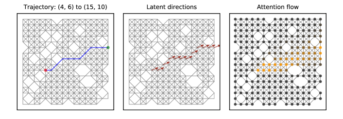
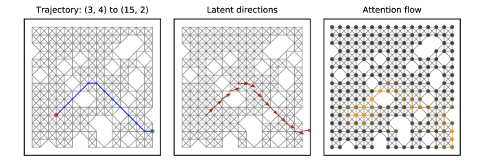
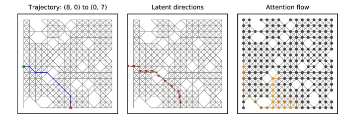
Figure 2: The true trajectory v.s. the latent directions in arrows v.s. the learned attention flow. The first row reflects a constant sloped direction, the second row time-dependent directions, the third row location-dependent directions, and the last row history-dependent directions. The drawn attention flow is based on the max aggregation of normalized attention distributions over the $T$ steps.

Objectives of comparison. We list our objectives of comparative evaluation from three aspects.

• To test how well the explicit attention flow modeling can leverage rich context carried by message passing in graph networks, compared to the modeling purely based on random walks.

• To test whether the backward acting of attention flow on message passing is useful, and which way can be the most effective.

• To test whether the explicit attention flow can improve the prediction accuracy.

Discussion on comparison results. First, we compare the models that explicitly model attention flow, between the random walk-based and the graph network-based. From Table 1 and 2, we see in most cases the models favored by graph networks surpass the random walk-based models, often by a large margin. Although there are exceptions that RW-Stationary performs strong in the location-dependent cases, probably due to little context needed other than current location information, the best of the graph network-based models, such as FullGN-MulMlp, can still beat it. Second, we compare the backward acting mechanism between no acting, the multiplying acting, and the non-linear acting. The non-linear acting after multiplying performs the best in almost all cases. What surprises us is that simply doing multiplying may degrade the performance, making it worse than no acting. How to design an effective backward acting mechanism is worth further study in future work. Last, we compare our remodeled graph networks with explicit attention flow against the regular graph networks. For the $32\times 32$ datasets, {FullGN,GGNN,GAT}-MulMlp exceed their regular graph network counterparts respectively except for dataset groups SINE-SZ32-STP16-*. For the larger $64\times 64$ datasets, we test GGNN and GGNN-MulMlp, and find that GGNN-MulMlp performs significantly much better than GGNN on every evaluation metric as shown in Table 3.

Discussion on visualization results. We visualize the learned attention flow in a $16\times 16$ corrupted grid map, compared with the true trajectories and latent directions by taking one example for each direction setting as shown in Figure 2. At first glance, the drawn attention flow over the $T$ steps makes up a belt linking from the source node to the destination node, almost matching the true trajectories, especially as shown in the first and second rows in Figure 2. On closer inspection, we find that the attention flow might not necessarily follow the one-path pattern but instead branch to enlarge the exploring area that is more likely to contain a destination node especially near gaps, as shown in the last two rows.

5 Conclusion

In this paper, we introduce the attention flow mechanism to explicitly model the reasoning process on graphs, leveraging the rich context carried by message passing in graph networks. We treat this mechanism as a way to offer accurate predictions as well as clear interpretations. In addition, we study the backward acting of attention flow on information flow implemented by message passing, and show some interesting findings from experimental results. The interaction between the two flows, one favoring the fitting capacity and one offering the interpretability, may be worth further study in future work.

Appendix

1 Experiments (cont’d)

Table 4: Parameters of generating the datasets

Dataset Group	$\vec{d}_{t,x,y}$	$N$	$T$	$\sigma$	$p_{\mathrm{node\_drp}}$	$p_{\mathrm{edge\_drp}}$
LINE-SZ32-STP16-NDRP-STD0.2	Line	32	16	0.2	0.1	0.0
LINE-SZ32-STP16-NDRP-STD0.5	Line	32	16	0.5	0.1	0.0
SINE-SZ32-STP16-NDRP-STD0.2	Sine	32	16	0.2	0.1	0.0
SINE-SZ32-STP16-NDRP-STD0.5	Sine	32	16	0.5	0.1	0.0
LOCATION-SZ32-STP16-NDRP-STD0.2	Location	32	16	0.2	0.1	0.0
LOCATION-SZ32-STP16-NDRP-STD0.5	Location	32	16	0.5	0.1	0.0
HISTORY-SZ32-STP16-NDRP-STD0.2	History	32	16	0.2	0.1	0.0
HISTORY-SZ32-STP16-NDRP-STD0.5	History	32	16	0.5	0.1	0.0
LINE-SZ32-STP16-EDRP-STD0.2	Line	32	16	0.2	0.0	0.2
LINE-SZ32-STP16-EDRP-STD0.5	Line	32	16	0.5	0.0	0.2
SINE-SZ32-STP16-EDRP-STD0.2	Sine	32	16	0.2	0.0	0.2
SINE-SZ32-STP16-EDRP-STD0.5	Sine	32	16	0.5	0.0	0.2
LOCATION-SZ32-STP16-EDRP-STD0.2	Location	32	16	0.2	0.0	0.2
LOCATION-SZ32-STP16-EDRP-STD0.5	Location	32	16	0.5	0.0	0.2
HISTORY-SZ32-STP16-EDRP-STD0.2	History	32	16	0.2	0.0	0.2
HISTORY-SZ32-STP16-EDRP-STD0.5	History	32	16	0.5	0.0	0.2
LINE-SZ64-STP32-NDRP-STD0.2	Line	64	32	0.2	0.1	0.0
LINE-SZ64-STP32-NDRP-STD0.5	Line	64	32	0.5	0.1	0.0
SINE-SZ64-STP32-NDRP-STD0.2	Sine	64	32	0.2	0.1	0.0
SINE-SZ64-STP32-NDRP-STD0.5	Sine	64	32	0.5	0.1	0.0
LOCATION-SZ64-STP32-NDRP-STD0.2	Location	64	32	0.2	0.1	0.0
LOCATION-SZ64-STP32-NDRP-STD0.5	Location	64	32	0.5	0.1	0.0
HISTORY-SZ64-STP32-NDRP-STD0.2	History	64	32	0.2	0.1	0.0
HISTORY-SZ64-STP32-NDRP-STD0.5	History	64	32	0.5	0.1	0.0

Table 5: Dataset statistics (All numbers represent average results. Note that dataset groups LINE-*-STD0.2 produce more trajectories per node than their counterparts, because the slop we choose makes the latent direction equally between two candidate edges, introducing more randomness to generate trajectories.)

Dataset Group	#Nodes	#Edges	#Trajs	#Trajs-per-node	Traj-length
LINE-SZ32-STP16-NDRP-STD0.2	921	6319	4829	5.2	9.1
LINE-SZ32-STP16-NDRP-STD0.5	921	6319	5029	5.5	9.0
SINE-SZ32-STP16-NDRP-STD0.2	921	6319	1555	1.7	9.0
SINE-SZ32-STP16-NDRP-STD0.5	921	6319	4380	4.8	9.4
LOCATION-SZ32-STP16-NDRP-STD0.2	921	6319	1440	1.6	7.9
LOCATION-SZ32-STP16-NDRP-STD0.5	921	6319	4098	4.4	8.8
HISTORY-SZ32-STP16-NDRP-STD0.2	921	6319	1541	1.7	8.5
HISTORY-SZ32-STP16-NDRP-STD0.5	921	6319	4418	4.8	9.2
LINE-SZ32-STP16-EDRP-STD0.2	1023	6248	4828	4.7	6.8
LINE-SZ32-STP16-EDRP-STD0.5	1023	6248	5051	4.9	6.7
SINE-SZ32-STP16-EDRP-STD0.2	1023	6248	1441	1.4	6.3
SINE-SZ32-STP16-EDRP-STD0.5	1023	6248	4238	4.1	6.8
LOCATION-SZ32-STP16-EDRP-STD0.2	1023	6248	1576	1.5	6.0
LOCATION-SZ32-STP16-EDRP-STD0.5	1023	6248	4327	4.2	6.6
HISTORY-SZ32-STP16-EDRP-STD0.	1023	6248	1586	1.5	6.0
HISTORY-SZ32-STP16-EDRP-STD0.	1023	6248	4441	4.3	6.6
LINE-SZ64-STP32-NDRP-STD0.2	3686	25891	21390	5.8	11.4
LINE-SZ64-STP32-NDRP-STD0.5	3686	25891	22106	6.0	11.1
SINE-SZ64-STP32-NDRP-STD0.2	3686	25891	6691	1.8	11.4
SINE-SZ64-STP32-NDRP-STD0.5	3686	25891	19233	5.2	11.7
LOCATION-SZ64-STP32-NDRP-STD0.2	3686	25891	6522	1.8	10.1
LOCATION-SZ64-STP32-NDRP-STD0.5	3686	25891	17482	4.7	10.8
HISTORY-SZ64-STP32-NDRP-STD0.2	3686	25891	6987	1.9	11.0
HISTORY-SZ64-STP32-NDRP-STD0.5	3686	25891	19303	5.2	11.7

1.1 Discussion about Results

During the experiments, we found some results in our expectation as discussed in the model section, as well as some unexpected results that surprise us, probably worth further study in future work. Now we summarize them as follows:

• Backward acting of attention flow on information flow is useful, better than no acting in most cases.

  • FullGN-{Mul,MulMlp} both perform better than FullGN-NoAct on Hits@1, Hits@5, Hits@10, MR and MRR for dataset groups LINE-SZ32-STP16-*, on Hits@1, Hits@5, Hits@10 and MRR for dataset groups SINE-SZ32-STP16-NDRP-STD0.2, SINE-SZ32-STP16-EDRP-*, LOCATION-SZ32-STP16-EDRP-STD0.5, on Hits@1 for dataset groups SINE-SZ32-STP16-NDRP-STD0.5, HISTORY-SZ32-STP16-*-STD0.2.

  • GGNN-{Mul,MulMlp} both perform better than GGNN-NoAct on Hits@1, Hits@5, Hits@10, MR and MRR for dataset group LINE-SZ32-STP16-NDRP-STD0.2, on Hits@1, MR and MRR for dataset group LINE-SZ32-STP16-NDRP-STD0.5, on Hits@1 and MRR for dataset groups HISTORY-SZ32-STP16-NDRP-*, on Hits@1 for dataset group SINE-SZ32-STP16-NDRP-STD0.5.

  • GAT-{Mul,MulMlp} both perform better than GAT-NoAct on Hits@1, Hits@5 and MRR for dataset groups SINE-SZ32-STP16-NDRP-STD0.2, LOCATION-SZ32-STP16-NDRP-STD0.5, HISTORY-SZ32-STP16-NDRP-STD0.5.

• Simply applying multiplying to backward acting might cause degradation.

  • {FullGN,GGNN,GAT}-Mul perform poorly on dataset groups LOCATION-SZ32-STP16-*.

  • {GGNN,GAT}-Mul perform poorly on dataset group SINE-SZ32-STP16-NDRP-STD0.5.

  • GGNN-Mul performs poorly on dataset group SINE-SZ32-STP16-NDRP-STD0.2.

• Non-linear backward acting after multiplying can work consistently well, always performing the best among the backward acting of NoAct, Mul and MulMlp, and even often the best among all the models.

  • {FullGN,GGNN,GAT}-MulMlp perform the best on Hits@1, Hits@5, MR and MR for dataset groups LINE-SZ32-STP16-*-STD0.2, on Hits@1 and MRR for dataset groups LOCATION-SZ32-STP16-*-STD0.2

  • {GGNN,GAT}-MulMlp perform the best on Hits@1, Hits@5 and MR for dataset groups LINE-SZ32-STP16-NDRP-STD0.5, HISTORY-SZ32-STP16-NDRP-STD0.5, on MR for dataset group SINE-SZ32-STP16-NDRP-STD0.2

  • {FullGN,GAT}-MulMlp perform the best on Hits@1, Hits@5, Hits@10 and MR for dataset group LOCATION-SZ32-STP16-NDRP-STD0.5, on MR for dataset group SINE-SZ32-STP16-NDRP-STD0.2, on MR and MRR for dataset group LINE-SZ32-STP16-NDRP-STD0.5

  • {FullGN,GGNN}-MulMlp perform the best on Hits@1 and MRR for dataset group HISTORY-SZ32-STP16-NDRP-STD0.2.

  • FullGN-MulMlp performs the best on Hits@1, Hits@5 and MRR for dataset groups LINE-SZ32-STP16-EDRP-STD0.2, LOCATION-SZ32-STP16-EDRP-*, on Hits@1 on dataset groups LINE-SZ32-STP16-EDRP-*, LOCATION-SZ32-STP16-EDRP-*, HISTORY-SZ32-STP16-EDRP-STD0.2, SINE-SZ32-STP16-EDRP-STD0.5, on MRR for dataset groups LINE-SZ32-STP16-EDRP-STD0.5, SINE-SZ32-STP16-EDRP-STD0.5, LOCATION-SZ32-STP16-EDRP-STD0.5

• Reasoning purely based on random walks with no message passing may be the worst in most cases, but in a few cases it can work surprisingly well.

  • RW-Stationary performs very poorly on dataset groups LINE-SZ32-STP16-NDRP-*, SINE-SZ32-STP16-NDRP-*, HISTORY-SZ32-STP16-NDRP-* but surprisingly well on dataset groups LOCATION-SZ32-STP16-NDRP-*. It is probably because under the location-dependent latent directions it requires little context except current location information to do the trajectory reasoning.

  • When considering global context information, RW-Dynamic works better than RW-Stationary in the cases where RW-Stationary performs poorly, but it obtains lower scores than RW-Stationary on dataset groups LOCATION-SZ32-STP16-NDRP-*, demonstrating again that little context is needed here.

• Regular graph networks work extremely well in the cases with the time-dependent latent directions, but they might not be suitable for other cases, such as the location-dependent and the history-dependent latent directions.

  • FullGN, GGNN, GAT obtain the highest scores and exceed the second by a large margin on dataset groups SINE-SZ32-STP16-* but still get a large MR score.

  • FullGN, GGNN, GAT perform very poorly on dataset groups LOCATION-SZ32-STP16-*, HISTORY-SZ32-STP16-* except GGNN on HISTORY-SZ32-STP16-NDRP-STD0.5.

• Models with attention flow taking non-linear backward acting might perform significantly better on a larger scale than those without.

  • From the results on dataset groups {LINE,SINE,LOCATION,HISTORY}-SZ64-STP32-NDRP-STD{0.2,0.5}, we can see GGNN-MulMlp surpasses GGNN by a large amount on every evaluation metric.

Table 6: Comparison results on dataset group LINE-SZ32-STP16-NDRP-STD0.2

Model	Hits@1 ($\%$)	Hits@5 ($\%$)	Hits@10 ($\%$)	MR	MRR
RW-Stationary	15.80 $\pm$0.56	56.95 $\pm$1.96	78.25 $\pm$2.31	9.857 $\pm$1.167	0.3409 $\pm$0.0098
RW-Dynamic	16.64 $\pm$0.65	59.65 $\pm$1.89	82.13 $\pm$1.77	7.061 $\pm$0.594	0.3562 $\pm$0.0084
FullGN	15.13 $\pm$0.74	59.75 $\pm$2.24	83.83 $\pm$1.99	6.800 $\pm$0.993	0.3451 $\pm$0.0082
FullGN-NoAct	16.65 $\pm$0.96	59.35 $\pm$2.08	82.50 $\pm$1.82	6.628 $\pm$0.392	0.3574 $\pm$0.0102
FullGN-Mul	16.69 $\pm$0.86	61.20 $\pm$1.66	83.58 $\pm$2.24	6.399 $\pm$0.609	0.3636 $\pm$0.0108
FullGN-MulMlp	16.99 $\pm$0.91	61.59 $\pm$2.05	83.73 $\pm$1.73	6.296 $\pm$0.615	0.3662 $\pm$0.0109
GGNN	15.49 $\pm$0.98	60.30 $\pm$1.80	83.60 $\pm$1.96	6.605 $\pm$0.580	0.3493 $\pm$0.0100
GGNN-NoAct	16.64 $\pm$0.86	59.62 $\pm$2.02	82.52 $\pm$1.53	6.760 $\pm$0.429	0.3570 $\pm$0.0095
GGNN-Mul	16.95 $\pm$0.70	59.80 $\pm$1.65	82.61 $\pm$2.05	6.477 $\pm$0.532	0.3610 $\pm$0.0089
GGNN-MulMlp	17.08 $\pm$0.77	61.45 $\pm$1.82	83.54 $\pm$1.89	6.316 $\pm$0.684	0.3673 $\pm$0.0111
GAT	16.01 $\pm$1.06	58.86 $\pm$1.82	80.78 $\pm$1.91	18.306 $\pm$16.927	0.3469 $\pm$0.0121
GAT-NoAct	16.02 $\pm$0.65	59.42 $\pm$1.95	82.29 $\pm$1.70	6.707 $\pm$0.397	0.3536 $\pm$0.0091
GAT-Mul	15.86 $\pm$0.99	58.77 $\pm$2.64	81.67 $\pm$1.98	6.518 $\pm$0.474	0.3501 $\pm$0.0122
GAT-MulMlp	17.07 $\pm$0.79	60.60 $\pm$1.70	83.22 $\pm$2.18	6.488 $\pm$0.670	0.3646 $\pm$0.0100

Table 7: Comparison results on dataset group LINE-SZ32-STP16-NDRP-STD0.5

Model	Hits@1 ($\%$)	Hits@5 ($\%$)	Hits@10 ($\%$)	MR	MRR
RW-Stationary	15.74 $\pm$0.54	55.28 $\pm$1.15	76.40 $\pm$1.24	10.087 $\pm$0.610	0.3348 $\pm$0.0040
RW-Dynamic	15.48 $\pm$0.82	57.07 $\pm$1.30	79.19 $\pm$1.04	7.735 $\pm$0.345	0.3429 $\pm$0.0071
FullGN	14.61 $\pm$0.90	57.97 $\pm$1.20	80.90 $\pm$1.02	8.472 $\pm$1.331	0.3355 $\pm$0.0090
FullGN-NoAct	15.50 $\pm$0.48	57.09 $\pm$1.31	79.55 $\pm$1.10	7.761 $\pm$0.416	0.3410 $\pm$0.0064
FullGN-Mul	16.21 $\pm$0.35	58.18 $\pm$1.45	80.73 $\pm$0.93	7.463 $\pm$0.284	0.3498 $\pm$0.0047
FullGN-MulMlp	16.07 $\pm$0.56	58.16 $\pm$1.02	80.59 $\pm$1.29	7.431 $\pm$0.283	0.3502 $\pm$0.0046
GGNN	14.53 $\pm$0.72	57.33 $\pm$1.01	80.34 $\pm$1.25	7.856 $\pm$0.669	0.3344 $\pm$0.0073
GGNN-NoAct	15.58 $\pm$0.53	57.44 $\pm$1.00	79.62 $\pm$1.17	7.789 $\pm$0.349	0.3415 $\pm$0.0055
GGNN-Mul	15.79 $\pm$0.63	57.36 $\pm$1.92	80.13 $\pm$1.16	7.387 $\pm$0.303	0.3448 $\pm$0.0060
GGNN-MulMlp	15.99 $\pm$0.59	58.17 $\pm$1.26	80.79 $\pm$0.98	7.391 $\pm$0.325	0.3497 $\pm$0.0052
GAT	14.79 $\pm$1.17	56.51 $\pm$2.26	79.20 $\pm$1.79	16.323 $\pm$12.684	0.3300 $\pm$0.0147
GAT-NoAct	15.83 $\pm$0.39	56.95 $\pm$1.25	79.28 $\pm$1.31	7.631 $\pm$0.309	0.3414 $\pm$0.0047
GAT-Mul	15.01 $\pm$0.84	55.95 $\pm$1.22	78.55 $\pm$1.62	7.793 $\pm$0.530	0.3351 $\pm$0.0071
GAT-MulMlp	16.25 $\pm$0.57	57.61 $\pm$1.35	80.60 $\pm$0.80	7.292 $\pm$0.190	0.3493 $\pm$0.0056

Table 8: Comparison results on dataset group SINE-SZ32-STP16-NDRP-STD0.2

Model	Hits@1 ($\%$)	Hits@5 ($\%$)	Hits@10 ($\%$)	MR	MRR
RW-Stationary	8.56 $\pm$1.76	35.81 $\pm$1.81	51.33 $\pm$2.47	23.883 $\pm$2.757	0.2177 $\pm$0.0103
RW-Dynamic	19.15 $\pm$3.02	50.69 $\pm$4.20	67.13 $\pm$3.58	13.554 $\pm$2.560	0.3418 $\pm$0.0266
FullGN	51.71 $\pm$3.46	87.46 $\pm$3.93	93.20 $\pm$4.78	17.588 $\pm$19.805	0.6665 $\pm$0.0348
FullGN-NoAct	30.10 $\pm$6.69	61.67 $\pm$7.22	76.88 $\pm$5.48	9.329 $\pm$2.224	0.4476 $\pm$0.0597
FullGN-Mul	37.49 $\pm$1.97	63.60 $\pm$2.72	76.91 $\pm$2.31	9.800 $\pm$1.077	0.4915 $\pm$0.0212
FullGN-MulMlp	39.91 $\pm$2.80	66.15 $\pm$3.01	78.19 $\pm$2.33	9.377 $\pm$0.824	0.5195 $\pm$0.0242
GGNN	51.02 $\pm$2.10	87.15 $\pm$3.44	93.51 $\pm$2.92	12.796 $\pm$18.578	0.6611 $\pm$0.0208
GGNN-NoAct	25.14 $\pm$6.53	54.30 $\pm$6.68	69.91 $\pm$4.57	12.509 $\pm$2.212	0.3918 $\pm$0.0604
GGNN-Mul	23.62 $\pm$2.30	53.62 $\pm$2.64	67.37 $\pm$3.12	15.002 $\pm$1.354	0.3776 $\pm$0.0168
GGNN-MulMlp	34.75 $\pm$2.93	60.76 $\pm$4.26	73.72 $\pm$3.33	12.392 $\pm$1.525	0.4699 $\pm$0.0264
GAT	43.19 $\pm$3.24	73.32 $\pm$3.67	79.30 $\pm$3.32	62.170 $\pm$12.886	0.5566 $\pm$0.0294
GAT-NoAct	15.77 $\pm$3.97	50.17 $\pm$4.34	67.36 $\pm$3.93	13.988 $\pm$1.933	0.3221 $\pm$0.0336
GAT-Mul	20.14 $\pm$2.10	50.70 $\pm$2.94	66.65 $\pm$2.81	15.725 $\pm$1.922	0.3429 $\pm$0.0193
GAT-MulMlp	30.64 $\pm$2.37	58.59 $\pm$3.91	73.46 $\pm$3.34	12.022 $\pm$1.639	0.4390 $\pm$0.0216

Table 9: Comparison results on dataset group SINE-SZ32-STP16-NDRP-STD0.5

Model	Hits@1 ($\%$)	Hits@5 ($\%$)	Hits@10 ($\%$)	MR	MRR
RW-Stationary	9.07 $\pm$0.60	34.71 $\pm$1.38	50.39 $\pm$3.15	19.937 $\pm$1.535	0.2267 $\pm$0.0090
RW-Dynamic	13.38 $\pm$1.06	46.26 $\pm$1.98	64.54 $\pm$2.05	12.380 $\pm$1.032	0.2905 $\pm$0.0103
FullGN	17.10 $\pm$0.67	57.91 $\pm$1.90	76.37 $\pm$1.58	9.517 $\pm$1.175	0.3525 $\pm$0.0069
FullGN-NoAct	16.60 $\pm$1.13	52.81 $\pm$1.95	71.91 $\pm$1.58	9.542 $\pm$0.790	0.3360 $\pm$0.0106
FullGN-Mul	16.93 $\pm$0.99	50.41 $\pm$1.98	67.74 $\pm$1.89	12.163 $\pm$0.526	0.3283 $\pm$0.0133
FullGN-MulMlp	17.31 $\pm$0.79	52.74 $\pm$1.68	70.69 $\pm$2.67	11.328 $\pm$1.042	0.3389 $\pm$0.0072
GGNN	17.45 $\pm$1.03	57.80 $\pm$1.59	76.72 $\pm$2.14	10.011 $\pm$1.730	0.3555 $\pm$0.0098
GGNN-NoAct	16.51 $\pm$1.51	50.63 $\pm$3.06	69.49 $\pm$2.48	10.611 $\pm$1.031	0.3262 $\pm$0.0163
GGNN-Mul	16.03 $\pm$1.21	50.61 $\pm$1.80	69.17 $\pm$2.34	11.253 $\pm$0.514	0.3226 $\pm$0.0156
GGNN-MulMlp	17.31 $\pm$1.55	53.07 $\pm$2.75	70.65 $\pm$1.08	11.500 $\pm$0.705	0.3370 $\pm$0.0177
GAT	16.48 $\pm$0.91	53.47 $\pm$1.60	71.89 $\pm$1.70	21.869 $\pm$12.869	0.3338 $\pm$0.0070
GAT-NoAct	15.15 $\pm$1.34	49.65 $\pm$3.17	68.24 $\pm$2.86	11.026 $\pm$1.152	0.3161 $\pm$0.0153
GAT-Mul	14.85 $\pm$0.90	48.34 $\pm$2.27	67.67 $\pm$2.24	11.681 $\pm$0.363	0.3070 $\pm$0.0097
GAT-MulMlp	16.45 $\pm$1.18	51.23 $\pm$2.81	68.86 $\pm$2.24	11.701 $\pm$0.526	0.3292 $\pm$0.0169

Table 10: Comparison results on dataset group LOCATION-SZ32-STP16-NDRP-STD0.2

Model	Hits@1 ($\%$)	Hits@5 ($\%$)	Hits@10 ($\%$)	MR	MRR
RW-Stationary	50.06 $\pm$3.23	84.70 $\pm$5.23	91.99 $\pm$3.76	5.997 $\pm$2.266	0.6625 $\pm$0.0403
RW-Dynamic	45.94 $\pm$6.63	85.81 $\pm$5.03	93.05 $\pm$2.62	6.036 $\pm$2.205	0.6320 $\pm$0.0544
FullGN	25.67 $\pm$8.66	69.33 $\pm$10.43	80.63 $\pm$7.18	18.589 $\pm$9.211	0.4393 $\pm$0.0884
FullGN-NoAct	46.47 $\pm$3.86	84.30 $\pm$3.88	92.22 $\pm$2.64	5.797 $\pm$2.316	0.6337 $\pm$0.0346
FullGN-Mul	43.44 $\pm$6.02	82.88 $\pm$5.66	89.49 $\pm$4.43	7.395 $\pm$2.546	0.6029 $\pm$0.0511
FullGN-MulMlp	50.93 $\pm$3.21	85.46 $\pm$4.93	91.03 $\pm$3.72	7.649 $\pm$3.921	0.6598 $\pm$0.0362
GGNN	29.20 $\pm$7.85	70.59 $\pm$8.83	79.83 $\pm$5.75	16.471 $\pm$6.033	0.4699 $\pm$0.0742
GGNN-NoAct	49.50 $\pm$3.91	87.84 $\pm$4.27	93.48 $\pm$3.09	5.850 $\pm$2.498	0.6621 $\pm$0.0383
GGNN-Mul	45.22 $\pm$4.67	83.48 $\pm$5.20	90.46 $\pm$3.57	8.098 $\pm$3.410	0.6185 $\pm$0.0437
GGNN-MulMlp	50.28 $\pm$3.36	86.41 $\pm$4.16	91.55 $\pm$3.27	6.634 $\pm$2.951	0.6637 $\pm$0.0342
GAT	18.18 $\pm$4.96	59.84 $\pm$6.92	73.31 $\pm$5.37	21.609 $\pm$3.249	0.3583 $\pm$0.0579
GAT-NoAct	46.10 $\pm$4.34	85.67 $\pm$4.78	92.54 $\pm$3.61	5.332 $\pm$1.829	0.6356 $\pm$0.0400
GAT-Mul	45.83 $\pm$2.74	82.99 $\pm$3.29	89.72 $\pm$2.19	7.059 $\pm$1.654	0.6208 $\pm$0.0232
GAT-MulMlp	47.52 $\pm$7.39	85.68 $\pm$4.04	92.97 $\pm$2.80	6.276 $\pm$2.278	0.6371 $\pm$0.0597

Table 11: Comparison results on dataset group LOCATION-SZ32-STP16-NDRP-STD0.5

Model	Hits@1 ($\%$)	Hits@5 ($\%$)	Hits@10 ($\%$)	MR	MRR
RW-Stationary	19.40 $\pm$1.03	64.37 $\pm$1.68	80.30 $\pm$1.63	9.569 $\pm$1.020	0.3860 $\pm$0.0113
RW-Dynamic	17.91 $\pm$0.75	62.47 $\pm$1.60	80.55 $\pm$1.87	9.379 $\pm$1.392	0.3722 $\pm$0.0101
FullGN	16.09 $\pm$1.51	58.99 $\pm$4.85	78.30 $\pm$4.49	16.608 $\pm$6.832	0.3476 $\pm$0.0256
FullGN-NoAct	18.83 $\pm$1.17	63.27 $\pm$1.71	82.63 $\pm$1.61	8.140 $\pm$0.986	0.3816 $\pm$0.0111
FullGN-Mul	18.50 $\pm$1.10	62.79 $\pm$1.96	81.34 $\pm$1.55	8.928 $\pm$1.070	0.3787 $\pm$0.0099
FullGN-MulMlp	19.64 $\pm$1.02	66.33 $\pm$1.75	83.87 $\pm$1.57	8.235 $\pm$1.025	0.3991 $\pm$0.0100
GGNN	17.11 $\pm$1.07	63.48 $\pm$2.29	81.83 $\pm$1.95	14.964 $\pm$3.551	0.3689 $\pm$0.0100
GGNN-NoAct	19.66 $\pm$0.81	64.74 $\pm$1.20	82.97 $\pm$0.98	8.118 $\pm$0.762	0.3912 $\pm$0.0086
GGNN-Mul	17.84 $\pm$1.11	62.36 $\pm$1.50	81.60 $\pm$2.31	9.220 $\pm$1.276	0.3723 $\pm$0.0114
GGNN-MulMlp	19.39 $\pm$0.60	65.81 $\pm$1.65	83.57 $\pm$1.40	8.375 $\pm$0.746	0.3911 $\pm$0.0061
GAT	14.51 $\pm$1.17	55.19 $\pm$2.14	72.87 $\pm$2.42	28.074 $\pm$4.756	0.3227 $\pm$0.0110
GAT-NoAct	17.82 $\pm$0.96	61.62 $\pm$1.47	80.28 $\pm$2.40	9.147 $\pm$1.037	0.3702 $\pm$0.0082
GAT-Mul	18.27 $\pm$0.73	62.42 $\pm$2.34	80.82 $\pm$1.26	9.260 $\pm$1.066	0.3749 $\pm$0.0093
GAT-MulMlp	18.93 $\pm$1.18	64.53 $\pm$1.90	83.06 $\pm$1.92	8.283 $\pm$0.988	0.3843 $\pm$0.0114

Table 12: Comparison results on dataset group HISTORY-SZ32-STP16-NDRP-STD0.2

Model	Hits@1 ($\%$)	Hits@5 ($\%$)	Hits@10 ($\%$)	MR	MRR
RW-Stationary	16.44 $\pm$3.08	47.22 $\pm$3.67	59.40 $\pm$4.04	34.573 $\pm$4.230	0.3215 $\pm$0.0319
RW-Dynamic	20.41 $\pm$2.07	55.07 $\pm$2.87	68.41 $\pm$2.77	24.968 $\pm$3.194	0.3656 $\pm$0.0206
FullGN	16.61 $\pm$4.79	48.68 $\pm$12.52	59.51 $\pm$14.14	63.999 $\pm$22.762	0.3095 $\pm$0.0765
FullGN-NoAct	20.80 $\pm$2.37	57.16 $\pm$3.94	70.07 $\pm$4.00	21.744 $\pm$3.576	0.3729 $\pm$0.0243
FullGN-Mul	21.35 $\pm$3.31	52.83 $\pm$3.56	64.58 $\pm$3.05	30.538 $\pm$3.866	0.3618 $\pm$0.0286
FullGN-MulMlp	23.94 $\pm$1.75	54.98 $\pm$3.86	65.76 $\pm$3.01	30.251 $\pm$5.933	0.3850 $\pm$0.0230
GGNN	22.56 $\pm$2.43	53.52 $\pm$3.10	62.88 $\pm$2.97	70.509 $\pm$11.580	0.3677 $\pm$0.0179
GGNN-NoAct	21.69 $\pm$2.26	57.50 $\pm$4.18	69.54 $\pm$3.70	24.676 $\pm$2.777	0.3818 $\pm$0.0186
GGNN-Mul	23.81 $\pm$2.21	54.66 $\pm$2.18	65.62 $\pm$2.62	29.538 $\pm$3.694	0.3824 $\pm$0.0175
GGNN-MulMlp	26.06 $\pm$1.51	56.04 $\pm$2.94	66.18 $\pm$3.54	32.089 $\pm$5.656	0.4001 $\pm$0.0173
GAT	12.11 $\pm$1.71	36.94 $\pm$3.05	47.97 $\pm$4.17	94.705 $\pm$8.713	0.2333 $\pm$0.0184
GAT-NoAct	23.17 $\pm$2.02	56.06 $\pm$3.09	68.00 $\pm$2.89	27.490 $\pm$3.953	0.3818 $\pm$0.0186
GAT-Mul	22.70 $\pm$2.58	56.12 $\pm$3.22	67.75 $\pm$3.05	30.113 $\pm$3.024	0.3762 $\pm$0.0188
GAT-MulMlp	20.71 $\pm$2.98	54.86 $\pm$2.76	66.01 $\pm$3.23	29.533 $\pm$5.556	0.3655 $\pm$0.0225

Table 13: Comparison results on dataset group HISTORY-SZ32-STP16-NDRP-STD0.5

Model	Hits@1 ($\%$)	Hits@5 ($\%$)	Hits@10 ($\%$)	MR	MRR
RW-Stationary	11.72 $\pm$2.02	41.07 $\pm$3.66	54.65 $\pm$4.07	34.876 $\pm$1.670	0.2547 $\pm$0.0231
RW-Dynamic	12.25 $\pm$1.39	46.04 $\pm$3.81	64.03 $\pm$3.78	20.600 $\pm$2.735	0.2820 $\pm$0.0191
FullGN	13.79 $\pm$1.65	51.04 $\pm$3.10	69.30 $\pm$2.87	31.874 $\pm$4.526	0.3051 $\pm$0.0207
FullGN-NoAct	13.90 $\pm$1.29	49.87 $\pm$2.94	67.39 $\pm$2.87	15.716 $\pm$1.772	0.3059 $\pm$0.0161
FullGN-Mul	12.93 $\pm$0.90	45.60 $\pm$2.75	61.88 $\pm$2.12	21.881 $\pm$2.319	0.2807 $\pm$0.0120
FullGN-MulMlp	14.89 $\pm$0.96	51.20 $\pm$2.36	68.48 $\pm$2.88	17.917 $\pm$2.680	0.3145 $\pm$0.0103
GGNN	14.83 $\pm$1.27	53.28 $\pm$3.22	70.76 $\pm$2.63	33.821 $\pm$7.460	0.3217 $\pm$0.0153
GGNN-NoAct	13.84 $\pm$1.21	48.51 $\pm$2.39	65.86 $\pm$2.34	20.799 $\pm$1.546	0.2957 $\pm$0.0126
GGNN-Mul	14.16 $\pm$1.06	47.27 $\pm$3.53	63.62 $\pm$3.58	23.457 $\pm$2.224	0.2971 $\pm$0.0168
GGNN-MulMlp	14.80 $\pm$1.26	49.47 $\pm$2.74	66.35 $\pm$3.00	22.230 $\pm$2.410	0.3053 $\pm$0.0142
GAT	10.80 $\pm$1.14	43.44 $\pm$2.81	60.12 $\pm$3.54	73.118 $\pm$7.201	0.2538 $\pm$0.0105
GAT-NoAct	12.60 $\pm$1.48	45.84 $\pm$3.56	62.84 $\pm$2.95	21.903 $\pm$1.581	0.2829 $\pm$0.0179
GAT-Mul	13.49 $\pm$1.28	46.23 $\pm$3.15	62.68 $\pm$2.85	23.887 $\pm$2.012	0.2885 $\pm$0.0149
GAT-MulMlp	13.75 $\pm$1.19	47.93 $\pm$2.72	64.23 $\pm$2.23	22.535 $\pm$1.538	0.2933 $\pm$0.0132

Table 14: Comparison results on dataset groups {LINE,SINE,LOCATION,HISTORY}-SZ32-STP16-EDRP-STD0.2

	Model	Hits@1 ($\%$)	Hits@5 ($\%$)	Hits@10 ($\%$)	MR	MRR
LINE	FullGN	17.59 $\pm$1.17	65.27 $\pm$2.71	85.47 $\pm$1.96	8.239 $\pm$1.769	0.3780 $\pm$0.0141
	-NoAct	19.39 $\pm$1.14	64.42 $\pm$2.06	83.84 $\pm$1.67	7.189 $\pm$0.458	0.3887 $\pm$0.0132
	-Mul	20.20 $\pm$1.28	65.51 $\pm$2.77	84.56 $\pm$2.30	6.260 $\pm$0.499	0.3985 $\pm$0.0145
	-MulMlp	20.26 $\pm$1.26	66.35 $\pm$2.87	84.88 $\pm$2.40	6.185 $\pm$0.501	0.3999 $\pm$0.0161
SINE	FullGN	63.08 $\pm$2.03	90.32 $\pm$2.38	93.16 $\pm$2.21	18.052 $\pm$5.502	0.7464 $\pm$0.0187
	-NoAct	52.87 $\pm$2.48	72.77 $\pm$4.75	81.82 $\pm$3.51	10.496 $\pm$2.357	0.6193 $\pm$0.0247
	-Mul	58.74 $\pm$2.14	75.56 $\pm$4.72	83.33 $\pm$3.38	7.518 $\pm$1.472	0.6681 $\pm$0.0281
	-MulMlp	56.94 $\pm$1.79	76.97 $\pm$2.38	83.37 $\pm$2.73	7.710 $\pm$1.647	0.6606 $\pm$0.0162
LOCA	FullGN	22.74 $\pm$5.22	68.86 $\pm$7.39	81.88 $\pm$4.49	20.447 $\pm$6.473	0.4213 $\pm$0.0554
	-NoAct	41.18 $\pm$2.98	82.45 $\pm$1.74	91.31 $\pm$1.61	5.390 $\pm$0.849	0.5881 $\pm$0.0249
	-Mul	37.69 $\pm$4.07	77.94 $\pm$4.28	87.52 $\pm$2.72	8.093 $\pm$1.841	0.5501 $\pm$0.0401
	-MulMlp	43.39 $\pm$3.26	84.32 $\pm$3.50	90.11 $\pm$3.15	6.249 $\pm$1.747	0.6081 $\pm$0.0297
HIST	FullGN	18.62 $\pm$2.96	61.12 $\pm$3.74	74.94 $\pm$3.95	32.250 $\pm$12.497	0.3648 $\pm$0.0264
	-NoAct	27.96 $\pm$2.04	65.73 $\pm$3.95	76.76 $\pm$3.44	13.564 $\pm$3.033	0.4494 $\pm$0.0200
	-Mul	28.40 $\pm$3.76	61.72 $\pm$5.35	72.94 $\pm$3.07	19.180 $\pm$3.192	0.4332 $\pm$0.0338
	-MulMlp	29.13 $\pm$2.91	62.26 $\pm$3.71	72.31 $\pm$3.65	18.469 $\pm$2.971	0.4416 $\pm$0.0297

Table 15: Comparison results on dataset groups {LINE,SINE,LOCATION,HISTORY}-SZ32-STP16-EDRP-STD0.5

	Model	Hits@1 ($\%$)	Hits@5 ($\%$)	Hits@10 ($\%$)	MR	MRR
LINE	FullGN	16.87 $\pm$1.85	63.11 $\pm$2.29	82.59 $\pm$1.53	9.296 $\pm$1.374	0.3669 $\pm$0.0177
	-NoAct	18.75 $\pm$1.67	62.33 $\pm$2.36	81.39 $\pm$2.00	8.564 $\pm$0.822	0.3764 $\pm$0.0189
	-Mul	19.42 $\pm$1.79	63.04 $\pm$2.25	81.63 $\pm$1.75	7.811 $\pm$0.684	0.3857 $\pm$0.0193
	-MulMlp	19.63 $\pm$1.85	63.03 $\pm$2.29	81.56 $\pm$1.59	8.029 $\pm$0.526	0.3867 $\pm$0.0198
SINE	FullGN	19.08 $\pm$1.11	62.90 $\pm$1.61	80.16 $\pm$1.61	18.303 $\pm$9.662	0.3759 $\pm$0.0117
	-NoAct	20.41 $\pm$1.61	56.18 $\pm$2.94	73.19 $\pm$3.01	11.914 $\pm$1.874	0.3656 $\pm$0.0160
	-Mul	21.53 $\pm$1.42	59.52 $\pm$2.30	75.77 $\pm$1.73	11.893 $\pm$1.124	0.3829 $\pm$0.0132
	-MulMlp	22.12 $\pm$1.21	60.09 $\pm$2.66	75.74 $\pm$1.96	12.262 $\pm$1.532	0.3884 $\pm$0.0134
LOCA	FullGN	15.95 $\pm$1.08	56.61 $\pm$2.39	76.61 $\pm$1.77	15.732 $\pm$4.803	0.3392 $\pm$0.0100
	-NoAct	18.55 $\pm$1.54	59.81 $\pm$2.67	78.41 $\pm$2.44	9.751 $\pm$1.260	0.3703 $\pm$0.0183
	-Mul	19.32 $\pm$1.14	60.34 $\pm$1.82	79.69 $\pm$1.92	10.382 $\pm$1.586	0.3759 $\pm$0.0136
	-MulMlp	19.36 $\pm$1.21	60.92 $\pm$2.14	80.31 $\pm$1.84	9.352 $\pm$1.572	0.3783 $\pm$0.0132
HIST	FullGN	14.00 $\pm$1.52	51.60 $\pm$2.51	70.76 $\pm$3.17	25.511 $\pm$6.818	0.3091 $\pm$0.0145
	-NoAct	16.61 $\pm$1.49	54.18 $\pm$2.26	70.87 $\pm$2.95	13.968 $\pm$1.772	0.3343 $\pm$0.0149
	-Mul	16.97 $\pm$0.94	50.46 $\pm$2.38	67.69 $\pm$1.77	16.933 $\pm$2.255	0.3252 $\pm$0.0123
	-MulMlp	16.27 $\pm$1.31	51.63 $\pm$3.22	68.57 $\pm$3.77	16.647 $\pm$2.403	0.3258 $\pm$0.0158

Table 16: Comparison results on dataset groups {LINE,SINE,LOCATION,HISTORY}-SZ64-STP32-NDRP-STD0.2

	Model	Hits@1 ($\%$)	Hits@5 ($\%$)	Hits@10 ($\%$)	MR	MRR
LINE	GGNN	12.12 $\pm$0.72	48.33 $\pm$1.56	72.83 $\pm$1.45	22.322 $\pm$13.982	0.2887 $\pm$0.0082
	-MulMlp	15.54 $\pm$0.24	54.61 $\pm$0.89	75.02 $\pm$0.89	8.863 $\pm$0.337	0.3324 $\pm$0.0040
SINE	GGNN	32.11 $\pm$3.73	65.53 $\pm$9.09	81.73 $\pm$5.49	52.180 $\pm$23.395	0.4681 $\pm$0.0494
	-MulMlp	38.21 $\pm$6.94	66.82 $\pm$4.65	76.14 $\pm$3.60	14.249 $\pm$2.623	0.5177 $\pm$0.0591
LOCA	GGNN	22.59 $\pm$4.28	72.54 $\pm$8.18	89.27 $\pm$4.67	14.619 $\pm$5.860	0.4335 $\pm$0.0515
	-MulMlp	44.01 $\pm$2.60	88.96 $\pm$2.30	95.94 $\pm$1.27	4.162 $\pm$0.978	0.6286 $\pm$0.0226
HIST	GGNN	9.99 $\pm$5.08	38.16 $\pm$18.57	56.51 $\pm$26.89	354.254 $\pm$620.045	0.2299 $\pm$0.1091
	-MulMlp	24.54 $\pm$1.77	57.98 $\pm$2.52	68.24 $\pm$2.39	49.187 $\pm$10.726	0.3931 $\pm$0.0205

Table 17: Comparison results on dataset groups {LINE,SINE,LOCATION,HISTORY}-SZ64-STP32-NDRP-STD0.5

	Model	Hits@1 ($\%$)	Hits@5 ($\%$)	Hits@10 ($\%$)	MR	MRR
LINE	GGNN	11.66 $\pm$0.70	47.09 $\pm$1.62	71.45 $\pm$1.10	22.898 $\pm$10.416	0.2814 $\pm$0.0082
	-MulMlp	14.95 $\pm$0.50	52.94 $\pm$1.55	73.01 $\pm$1.19	10.949 $\pm$0.683	0.3231 $\pm$0.0070
SINE	GGNN	10.47 $\pm$0.99	39.78 $\pm$4.60	61.11 $\pm$5.50	29.445 $\pm$12.722	0.2484 $\pm$0.0209
	-MulMlp	16.68 $\pm$0.59	50.91 $\pm$1.88	67.42 $\pm$1.59	17.379 $\pm$1.724	0.3238 $\pm$0.0099
LOCA	GGNN	11.80 $\pm$1.37	45.93 $\pm$4.26	69.08 $\pm$5.12	26.319 $\pm$8.972	0.2784 $\pm$0.0224
	-MulMlp	18.51 $\pm$0.51	62.85 $\pm$1.29	82.41 $\pm$1.07	8.423 $\pm$0.738	0.3778 $\pm$0.0059
HIST	GGNN	7.65 $\pm$0.98	32.67 $\pm$3.84	53.00 $\pm$5.57	92.365 $\pm$19.973	0.2064 $\pm$0.0192
	-MulMlp	13.47 $\pm$0.74	45.79 $\pm$2.11	62.85 $\pm$2.35	39.793 $\pm$5.507	0.2839 $\pm$0.0125

1.2 More Visualization Results

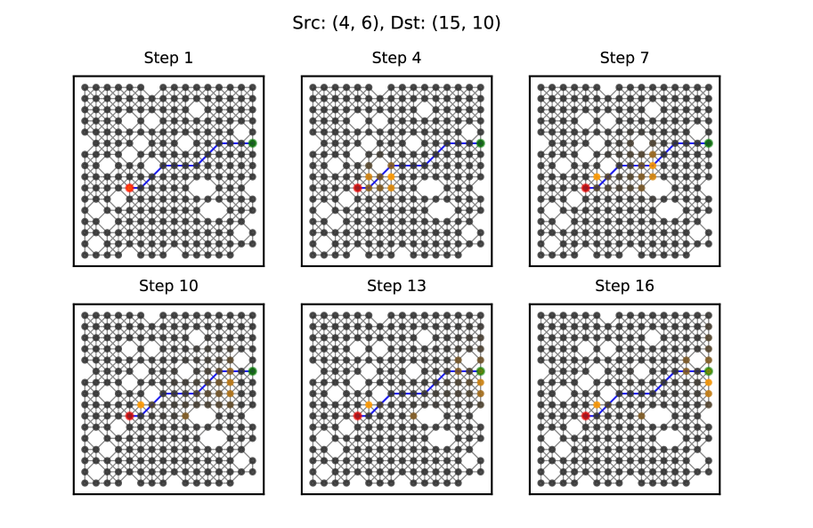
Figure 3: Attention distributions at different steps. The latent directions follow a straight line.

Figure 4: Attention distributions at different steps. The latent directions follow a sine curve, depending on time.

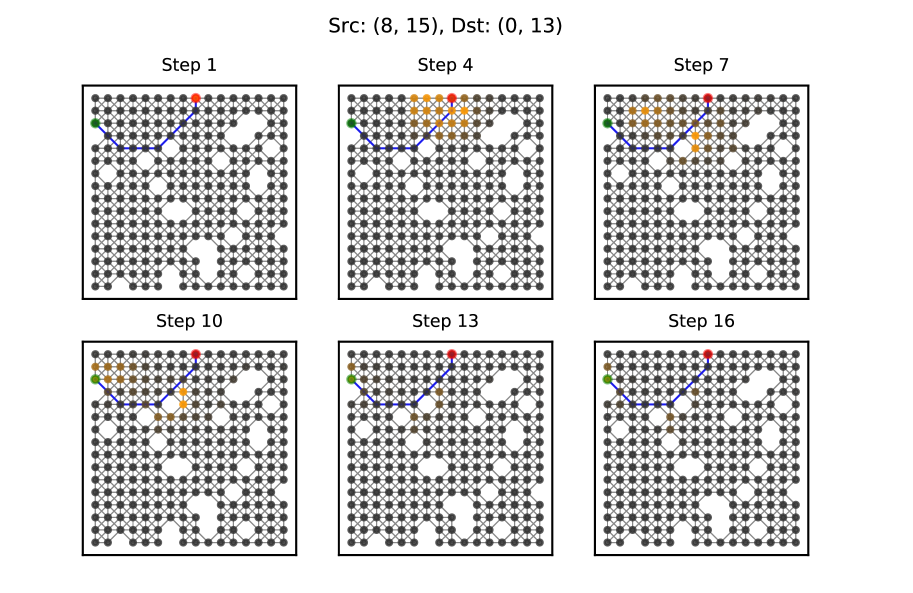
Figure 5: Attention distributions at different steps. The latent directions depend on current locations.

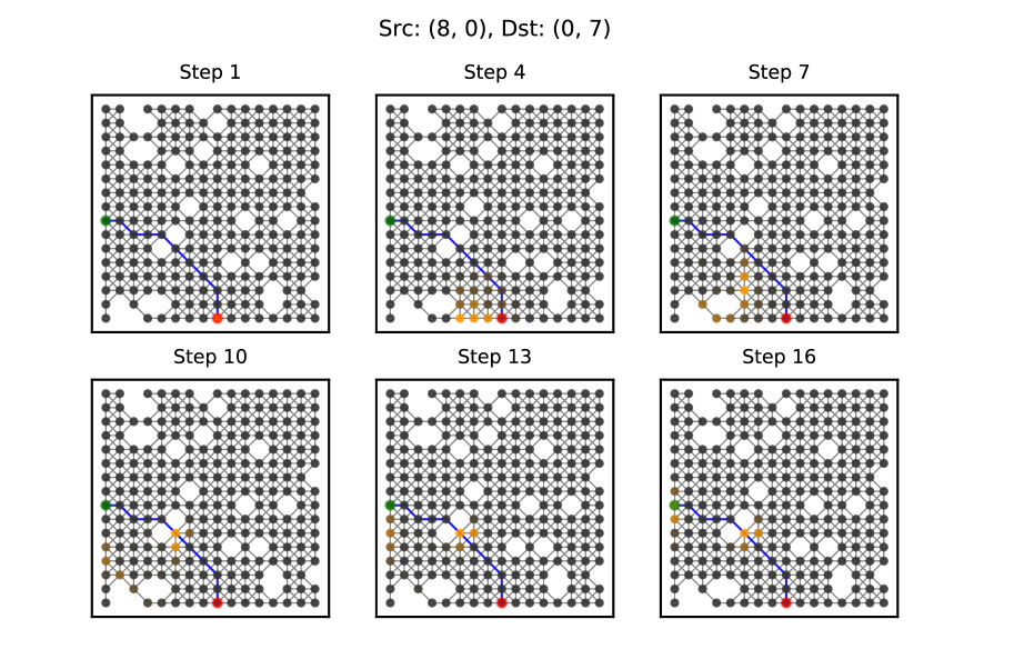
Figure 6: Attention distributions at different steps. The latent directions depend on location history.

References

- [1] Marco Gori, Gabriele Monfardini, and Franco Scarselli. A new model for learning in graph domains. In Neural Networks, 2005. IJCNN’05. Proceedings. 2005 IEEE International Joint Conference on, volume 2, pages 729–734. IEEE, 2005.
- [2] Franco Scarselli, Marco Gori, Ah Chung Tsoi, Markus Hagenbuchner, and Gabriele Monfardini. The graph neural network model. IEEE Transactions on Neural Networks, 20(1):61–80, 2009.
- [3] Peter W Battaglia, Jessica B Hamrick, Victor Bapst, Alvaro Sanchez-Gonzalez, Vinicius Zambaldi, Mateusz Malinowski, Andrea Tacchetti, David Raposo, Adam Santoro, Ryan Faulkner, et al. Relational inductive biases, deep learning, and graph networks. arXiv preprint arXiv:1806.01261, 2018.
- [4] Alvaro Sanchez-Gonzalez, Nicolas Heess, Jost Tobias Springenberg, Josh Merel, Martin Riedmiller, Raia Hadsell, and Peter Battaglia. Graph networks as learnable physics engines for inference and control. arXiv preprint arXiv:1806.01242, 2018.
- [5] Jessica B Hamrick, Kelsey R Allen, Victor Bapst, Tina Zhu, Kevin R McKee, Joshua B Tenenbaum, and Peter W Battaglia. Relational inductive bias for physical construction in humans and machines. arXiv preprint arXiv:1806.01203, 2018.
- [6] William W Cohen. Tensorlog: A differentiable deductive database. arXiv preprint arXiv:1605.06523, 2016.
- [7] William W Cohen, Fan Yang, and Kathryn Rivard Mazaitis. Tensorlog: Deep learning meets probabilistic dbs. arXiv preprint arXiv:1707.05390, 2017.
- [8] Fan Yang, Zhilin Yang, and William W Cohen. Differentiable learning of logical rules for knowledge base reasoning. In Advances in Neural Information Processing Systems, pages 2319–2328, 2017.
- [9] Yujia Li, Daniel Tarlow, Marc Brockschmidt, and Richard Zemel. Gated graph sequence neural networks. arXiv preprint arXiv:1511.05493, 2015.
- [10] Peter Battaglia, Razvan Pascanu, Matthew Lai, Danilo Jimenez Rezende, et al. Interaction networks for learning about objects, relations and physics. In Advances in neural information processing systems, pages 4502–4510, 2016.
- [11] David Raposo, Adam Santoro, David Barrett, Razvan Pascanu, Timothy Lillicrap, and Peter Battaglia. Discovering objects and their relations from entangled scene representations. arXiv preprint arXiv:1702.05068, 2017.
- [12] Justin Gilmer, Samuel S Schoenholz, Patrick F Riley, Oriol Vinyals, and George E Dahl. Neural message passing for quantum chemistry. arXiv preprint arXiv:1704.01212, 2017.
- [13] Petar Velickovic, Guillem Cucurull, Arantxa Casanova, Adriana Romero, Pietro Lio, and Yoshua Bengio. Graph attention networks. arXiv preprint arXiv:1710.10903, 2017.
- [14] Xiaolong Wang, Ross Girshick, Abhinav Gupta, and Kaiming He. Non-local neural networks. In The IEEE Conference on Computer Vision and Pattern Recognition (CVPR), 2018.
- [15] Michael M Bronstein, Joan Bruna, Yann LeCun, Arthur Szlam, and Pierre Vandergheynst. Geometric deep learning: going beyond euclidean data. IEEE Signal Processing Magazine, 34(4):18–42, 2017.
- [16] Joan Bruna, Wojciech Zaremba, Arthur Szlam, and Yann LeCun. Spectral networks and locally connected networks on graphs. arXiv preprint arXiv:1312.6203, 2013.
- [17] Mikael Henaff, Joan Bruna, and Yann LeCun. Deep convolutional networks on graph-structured data. arXiv preprint arXiv:1506.05163, 2015.
- [18] Michaël Defferrard, Xavier Bresson, and Pierre Vandergheynst. Convolutional neural networks on graphs with fast localized spectral filtering. In Advances in Neural Information Processing Systems, pages 3844–3852, 2016.
- [19] Thomas N Kipf and Max Welling. Semi-supervised classification with graph convolutional networks. arXiv preprint arXiv:1609.02907, 2016.
- [20] David K Duvenaud, Dougal Maclaurin, Jorge Iparraguirre, Rafael Bombarell, Timothy Hirzel, Alán Aspuru-Guzik, and Ryan P Adams. Convolutional networks on graphs for learning molecular fingerprints. In Advances in neural information processing systems, pages 2224–2232, 2015.
- [21] Mathias Niepert, Mohamed Ahmed, and Konstantin Kutzkov. Learning convolutional neural networks for graphs. In International conference on machine learning, pages 2014–2023, 2016.
- [22] Federico Monti, Davide Boscaini, Jonathan Masci, Emanuele Rodola, Jan Svoboda, and Michael M Bronstein. Geometric deep learning on graphs and manifolds using mixture model cnns. In Proc. CVPR, volume 1, page 3, 2017.
- [23] James Atwood and Don Towsley. Diffusion-convolutional neural networks. In Advances in Neural Information Processing Systems, pages 1993–2001, 2016.
- [24] Will Hamilton, Zhitao Ying, and Jure Leskovec. Inductive representation learning on large graphs. In Advances in Neural Information Processing Systems, pages 1024–1034, 2017.
- [25] Rajarshi Das, Shehzaad Dhuliawala, Manzil Zaheer, Luke Vilnis, Ishan Durugkar, Akshay Krishnamurthy, Alex Smola, and Andrew McCallum. Go for a walk and arrive at the answer: Reasoning over paths in knowledge bases using reinforcement learning. arXiv preprint arXiv:1711.05851, 2017.
- [26] Elias Khalil, Hanjun Dai, Yuyu Zhang, Bistra Dilkina, and Le Song. Learning combinatorial optimization algorithms over graphs. In Advances in Neural Information Processing Systems, pages 6348–6358, 2017.
- [27] Irwan Bello, Hieu Pham, Quoc V Le, Mohammad Norouzi, and Samy Bengio. Neural combinatorial optimization with reinforcement learning. arXiv preprint arXiv:1611.09940, 2016.
- [28] Dzmitry Bahdanau, Kyunghyun Cho, and Yoshua Bengio. Neural machine translation by jointly learning to align and translate. arXiv preprint arXiv:1409.0473, 2014.
- [29] Ashish Vaswani, Noam Shazeer, Niki Parmar, Jakob Uszkoreit, Llion Jones, Aidan N Gomez, Łukasz Kaiser, and Illia Polosukhin. Attention is all you need. In Advances in Neural Information Processing Systems, pages 5998–6008, 2017.
- [30] WWM Kool and M Welling. Attention solves your tsp. arXiv preprint arXiv:1803.08475, 2018.
- [31] Eric Jang, Shixiang Gu, and Ben Poole. Categorical reparameterization with gumbel-softmax. arXiv preprint arXiv:1611.01144, 2016.
- [32] Chris J Maddison, Andriy Mnih, and Yee Whye Teh. The concrete distribution: A continuous relaxation of discrete random variables. arXiv preprint arXiv:1611.00712, 2016.