Optimal 1D Trajectory Design for UAV-Enabled Multiuser Wireless Power Transfer ††thanks: *J. Xu is the corresponding author.
Abstract
In this paper, we study an unmanned aerial vehicle (UAV)-enabled wireless power transfer (WPT) network, where a UAV flies at a constant altitude in the sky to provide wireless energy supply for a set of ground nodes with a linear topology. Our objective is to maximize the minimum received energy among all ground nodes by optimizing the UAV’s one-dimensional (1D) trajectory, subject to the maximum UAV flying speed constraint. Different from previous works that only provided heuristic and locally optimal solutions, this paper is the first work to present the globally optimal 1D UAV trajectory solution to the considered min-energy maximization problem. Towards this end, we first show that for any given speed-constrained UAV trajectory, we can always construct a maximum-speed trajectory and a speed-free trajectory, such that their combination can achieve the same received energy at all these ground nodes. Next, we transform the original UAV-speed-constrained trajectory optimization problem into an equivalent UAV-speed-free problem, which is then optimally solved via Lagrange dual method. The obtained optimal 1D UAV trajectory solution follows the so-called successive hover-and-fly (SHF) structure, i.e., the UAV successively hovers at a finite number of hovering points each for an optimized hovering duration, and flies among these hovering points at the maximum speed. Numerical results show that our proposed optimal solution significantly outperforms the benchmark schemes in prior works under different scenarios.
Index Terms:
Unmanned aerial vehicle (UAV), wireless power transfer (WPT), energy fairness, trajectory optimization, successive hover-and-fly (SHF).I Introduction
In recent years, unmanned aerial vehicle (UAV)-enabled wireless applications have attracted increasing attentions, as UAVs can be used for the quick deployment of on-demand wireless systems. Thanks to the presence of line-of-sight (LoS) aerial-to-ground wireless links between UAVs and ground devices, UAV-enabled wireless networks are likely to have a better system performance than conventional terrestrial wireless networks [1]. In general, there are two types of UAV-enabled wireless applications, i.e., wireless communication [2, 3, 4, 5, 6, 7, 8, 9] and wireless power transfer (WPT) [10, 12, 11, 13].
In UAV-enabled wireless communication, the fully mobile UAVs provide new degrees of freedom in improving the wireless performance via optimizing UAVs’ quasi-stationary deployment locations or time-varying locations over time (a.k.a. trajectories) [2]. For instance, the prior works [6, 7, 8, 9, 5] considered UAV-enabled cellular base stations (BSs), where the UAV’s deployment locations are optimized to provide the maximum coverage for ground users [6, 7, 8, 9], and to enhance the performance of cell-edge users via data offloading [5]. In addition, in UAV-enable mobile relaying systems, the UAV trajectory is jointly optimized with the wireless resource allocation, so as to maximize the throughput [3, 14] or the energy efficiency [4].
On the other hand, motivated by the great success of integrating WPT into wireless networks [15, 16, 17], UAV-enabled WPT has recently emerged as a promising solution to prolong the lifetime of low-power sensors and IoT devices, by using UAVs as mobile energy transmitters (ETs) to power these devices [10, 12, 11, 13]. In particular, by considering the UAV flying at a fixed altitude, the works [10, 12] optimized the one-dimensional (1D) or two-dimensional (2D) UAV trajectory to maximize the energy transfer performance for a UAV-enabled WPT network, subject to a maximum UAV speed constraints. In a two-user scenario in a linear topology, the authors in [10] optimized the 1D UAV trajectory to characterize the Pareto boundary of the achievable energy region by the two users. This result is then extended to the general multiuser scenario in a 2D topology in [12], where the 2D UAV trajectory is optimized to maximize the minimum received energy among these users. It is worth noting that the above approaches in [10, 12] can only obtain the globally optimal solution in the extreme case with the UAV maximum speed constraints being ignored. For the general case with the UAV maximum speed constraints involved, these approaches can only obtain heuristic and locally optimal solutions. To our best knowledge, for the UAV-enabled WPT networks, how to obtain the optimal UAV trajectory solution and reveal its structure still remains unknown, even for the basic case with two users in a linear topology. This thus motivates our investigation in this paper to provide an optimal 1D UAV trajectory design and to characterize the structure of the optimal UAV trajectory.
In this paper, we consider a UAV-enabled WPT network with a linear topology, where multiple ground nodes are deployed in a straight line, e.g., along with a river, road or tunnel. To charge these ground nodes in an efficient and fair manner, we aim at maximizing the minimal received energy among all ground nodes via designing the UAV’s 1D trajectory (or equivalently the velocity) for WPT, while the UAV mobility is subject to maximum speed constraints. The results of this work are summarized as follows: Different from previous works that only provided heuristic and locally optimal solutions, for the first time, we present the globally optimal 1D UAV trajectory solution to the considered WPT problem, by equivalently decomposing any speed-constrained 1D UAV trajectory into a maximum-speed trajectory and a speed-free trajectory, together with the Lagrange dual method. It is proved that the optimal 1D UAV trajectory solution follows an interesting successive hover-and-fly (SHF) structure, i.e., the UAV successively hovers at a finite number of hovering points each for an optimized hovering duration, and flies among these hovering points at the maximum speed.
II System Model and Problem Formulation
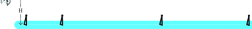
In this paper, we consider a UAV-enabled multiuser WPT system with a linear topology as shown in Fig. 1, where a UAV flies at a fixed altitude to wirelessly charge a set of ground nodes (such as IoT devices and sensors) that are located in a straight line.
We denote the horizontal location of node as . We assume that without loss of generality. To efficiently charge all nodes, we focus on a finite UAV charging period with duration . The UAV’s time-varying horizontal location is denoted by at time instant . In addition, the UAV is subject to a maximal flying speed . Hence, we have , where denotes the first-order derivative of .
In practice, the wireless channels between the UAV and ground nodes are LoS-dominant, and therefore, we adopt the free-space path loss model as normally used in the UAV-enabled wireless communication and WPT literature [3]. At time , the channel power gain from the UAV to ground node is denoted as , where the distance between the UAV and ground node is and is the channel power gain at a reference distance of unit meter. Hence, the received radio frequency (RF) power by ground node at time is
| (1) |
where denotes the constant transmit power of the UAV. Notice that in practice, the received radio frequency (RF) signal should be converted into a direct current (DC) signal to charge the rechargeable battery at each ground node, and the RF-to-DC conversion is in general a non-linear process [18]. In order to focus our study on the wireless transmission, we use the received RF power as the performance metric by ignoring the non-linear RF-to-DC conversion process, as in [10, 12].
Due to the broadcast nature of the wireless transmission, all ground nodes can simultaneously receive wireless power during the whole charging period . As a result, the total energy received by ground node is given by
| (2) |
Our objective is to design the UAV trajectory to maximize the minimal received energy among all the nodes during the charging period . The problem is formulated as
| (3) | |||||
By introducing an auxiliary variable , the original problem (OP) is equivalently reformulated as
Notice that both the original problem (OP) and the reformulated problem (P1) are non-convex, due to the fact that the objective function in (OP) is non-concave, and constraint in (P1) is non-convex, respectively. Furthermore, both problems consist of an infinite number of variables over continuous time. Therefore, how to find the optimal solution to the min-energy maximization problem is generally a very difficult task.
Notice that in the prior work [12], the authors solved the 2D UAV trajectory optimization problem for min-energy maximization by the following three-step approach, which can also be used to solve (OP) and (P1) directly. First, by considering a relaxed problem of (P1) with the UAV’s maximum speed constraint ignored, the optimal multi-location-hovering trajectory solution of the relaxed problem is obtained. Next, by taking into account the maximum UAV speed constraint, a heuristic SHF trajectory design is proposed, in which the UAV flies at the maximum speed to successively visit the obtained optimal hovering locations to the relaxed problem above, and hovers above them accordingly. In the heuristic SHF trajectory, the traveling salesmen problem (TSP) is used to obtain the visiting order among these locations with minimized flying distance/time111Note that TSP is only needed for the 2D trajectory, but is not required for the 1D trajectory design of our interest. Nevertheless, the heuristic SHF is suboptimal as it does not take into account the WPT during UAV flying. . Finally, the successive convex approximation (SCA)-based trajectory design is proposed, which quantizes the path or time to subsequently refine the trajectory towards a locally optimal solution. It is worth noting that both the heuristic SHF and the SCP based approaches can only obtain the globally optimal solution the relaxed problem, which mathematically corresponds to the ideal case with the flying duration or the UAV flying speed being infinite. This case may not happen in practice. For the general case, the heuristic SHF trajectory is suboptimal, while the performance of the SCP-based trajectory can only ensure the local optimality when the quantization becomes extremely accurate. How to characterize the optimal 1D UAV trajectory solution to the min-energy maximization problem in the general case with speed constraints is still unknown.
III Optimal SHF Trajectory Solution
In this section, we present the optimal trajectory solution to problem (OP) or (P1), and show that it has an interesting SHF structure, in which the UAV hovers among a number of locations and then flies among them at the maximum speed.
First, notice that there always exists a uni-directional trajectory that is optimal for problem (P1), i.e., This is due to the fact that for any given trajectory, we can always find an alternative uni-directional UAV trajectory to achieve the same WPT performance but without flying forward and backward [19]. Therefore, in this paper we focus on the uni-directional trajectory without loss of optimality.
Next, we consider problem (P1) under given pair of initial and final locations . This sub-problem is expressed as
In the following, we first show that any speed-constrained trajectory to problem (P1.1) is mathematically equivalent to the combination of a maximum-speed trajectory and a speed-free trajectory, and then provide the optimal solution to problem (P1.1) under any given and via the Lagrange dual method. After that, we obtain the optimal solution to problem (P1) by applying a 2D exhaustive search over , .
III-A Problem Reformulation
We start with the following lemma to show that we can construct two trajectories for any unidirectional trajectory satisfying the maximum speed .
Lemma 1.
For any duration- unidirectional trajectory satisfying the maximum speed with given initial position and final position , we can always find two UAV trajectories and to jointly achieve the same WPT performance. In particular, is the max-speed flying with , where . In addition, has a time duration without any UAV speed constraints (speed-free). In other words, the following equality holds for any .
| (6) |
Proof.
The proof is provided in Appendix A. ∎
Note that for the maximum-speed flying trajectory from to , the trajectory is fixed, i.e., the UAV flies from to at the maximal speed . In particular, for trajectory , the received energy by ground node is
| (7) |
III-B Optimal Solution to Problem (P2)
Problem (P2) is non-convex but satisfies the so-called time-sharing condition in [21]. Therefore, strong duality holds between problem (P2) and its Lagrange dual problem. Therefore, problem (P2) can be solved via the Lagrange dual method [22].
Denote the Lagrange multiplier for the -th constraint in (8) by . The partial Lagrangian of problem (P2) is
| (9) |
Immediately, we have the corresponding dual function as
Clearly, the condition must be satisfied to guarantee that the function is upper-bounded from above, i.e., . Otherwise, if (or ), we have by setting (or ). Then, the dual problem of problem (P2) is given by
| (11) | |||||
| (12) |
Notice that as strong duality holds between problem (P2) and its dual problem (DP2), we solve problem (P2) by equivalently solving the dual problem (DP2), in which we first obtain the dual function under any given by solving problem (III-B), and then updating via subgradient-based methods such as the ellipsoid method [20] to find the opitmal maximizing .
First of all, we deteminate the dual function . Consider problem (III-B) under any given satisfying the constraints in (DP2). As , problem (10) can be decomposed into the following subproblems by dropping the constant term , each for one time instant .
| (13) | |||||
As the problem in (13) has the same form at different time instant in the above problem, we can simply drop the variable and re-express the problem as
| (14) | |||||
We obtain the extreme points of by letting its first order derivative be zero, i.e.,
| (15) |
which equals to solve
| (16) |
In other words, the extreme points of can be obtained by solving (16). By comparing the objective values in (III-B) at the extreme points versus those at the boundary points and , the optimal hovering points , are obtained, where denotes the number of optimal solutions which achieves the same objective value. Accordingly, the dual function is obtained.
With obtained, the dual problem (DP2) can be solved via the ellipsoid method, and therefore, the solution is obtained. Based on , we can reconstruct the primal optimal solution to (P2) by solving the time-sharing problem for allocating the total duration over the hovering points, for which the optimization problem is formulated as the following linear program (LP):
By solving this LP problem via standard interior point method, we obtain the optimal hovering durations , corresponding to the hovering points. Therefore, (P2) is optimally solved under the given and . In summary, the optimal solution to (P2) is described by the optimal hovering points and hovering durations
| (18) |
where .
Lemma 2.
There exists one optimal multi-location-hovering solution to problem (P2) with the number of hovering points being no more than , i.e., .
Proof.
It is observed that the optimal solution to (P2) has a multi-location-hovering structure, i.e., the solution to problem (III-B) is a set of hovering points. Note that the left side of (16) is a order polynomial of , i.e., has at most extrema and therefore at most maximum points as potential hovering points. In addtioin, the two boundary points and are also potential hovering points. Hence, there are a maximum number of hovering locations in the optimal solution to (P2). ∎
III-C Optimal Solution to Problem (P1.1)
In Section III-B, we have shown that for given and , the global optimal trajectory problem (P2) can be obtained. Suppose that the corresponding optimal solution to problem (P2) with optimal hovering points , and the corresponding optimal hovering durations. , . According to Lemma 1, we can express the optimal solution to (P1.1) by combining with , i.e., letting the UAV fly at the maximal speed from to while stopping/hovering at the hovering points (in between) with the corresponding optimal hovering durations. By defining , and , we have the optimal solution to problem (P1.1), where is given in (12).
III-D Optimal Solution to (OP) or (P1)
In Section III-D, we have shown that the global optimal trajectory to problem (P1.1) is obtained, i.e., we have optimally solved problem (P1) under given and . Hence, by applying a 2D exhaustive search over the possible pair of and together with solving (P1.1) under each and , the global optimally trajectory solution to problem (P1) is finally obtained. It is clear there is no benefit if the UAV hovers at a position out of the region of ground nodes. Hence, the feasible set of is while the corresponding feasible set of is . To apply the exhaustive search on or within its continuous feasible set, we introduce as the resolution in distance. Note that we have should be small and let be an integer. Hence, the feasible locations of and the corresponding become and , respectively.
The detail description of the optimal solution to (P1) is provided in Algorithm 1.
III-E Structure of the Optimal Trajectory to Problem (P1)
We describe the structure of the optimal trajectory solution to problem (P1) in the following proposition.
Proposition 1.
The optimal trajectory solution to problem (P1.1) or problem (P1) follows the SHF structure, i.e., there exists a number of hovering locations at the optimal trajectory, such that the UAV always flies at the maximum speed from one hovering location to another, and then hovers at that location for a certain time duration. It then holds that .
Proof.
Combining Lemmas 1 and 2, this proposition is verified directly for problem (P1.1). Note that the global optimal trajectory to problem (P1) is obtained by applying a 2D exhaustive search over the possible pair of and , i.e., the optimal solution to problem (P1) is the best one in the solutions of all the problems (P1.1) with different and . Hence, as the optimal solution to any problem (P1.1) has a SHF structure, the global optimal trajectory to problem (P1) also has such a structure, i.e., Proposition 1 holds also for problem (P1). ∎
IV Numerical Results
In this section, we evaluate the proposed optimal SHF algorithm, in comparison to two reference algorithm, i.e., the heuristic SHF and the SCP with time quantization from [12]. To obtain the WPT performance, we randomly drop ground nodes to have different topologies, and then apply these three algorithms at each topology, and finally average the max-min received power among all ground nodes over these random realizations. In the simulation, we have the following default setups of parameters: , , , , , and is a -dimension vector with each element being a random number in interval , where . In addition, we set the quantization size of distance for the exhaustive search in the proposed algorithms to and set accordingly the time quantization size in the reference algorithm SCP with time quantization to .
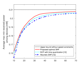

We first study the impact of the charging duration on the max-min received power (among all ground nodes). The results are shown in Fig. 2, where the upper bound of the ideal case with UAV speed constraint ignored is also provided. First, it is observed that, as the charging duration increases, the performance of all the three algorithms increases towards the upper bound. In addition, owning to applying additional SCP process, the SCP with time quantization has a better performance than the heuristic SHF, which is consistent with the results in [12]. More importantly, the proposed optimal SHF outperforms the two reference algorithms, in the whole charging duration regime.
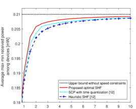
The relationship between the max-min received power (among all ground nodes) and UAV speed is investigated in Fig. 3. From the figure, we learn that under all algorithms, the max-min received power increases as the UAV speed becomes large. In addition, as the speed significantly increases, all the three designs are observed to approach the upper bound. Moreover, we observe again the performance advantage of the proposed optimal algorithm in comparison to the two reference algorithms.
V Conclusion
In this paper, we focus on a UAV-enabled multiuser WPT network with a linear topology. We studied the 1D UAV trajectory design problem with the objective of maximizing the minimal received energy among all ground nodes, subject to the maximum UAV speed constraints. Different from previous works that only provided heuristic and locally optimal solutions, for the first time, we presented the globally optimal 1D UAV trajectory solution to the considered WPT problem, by equivalently decomposing any speed-constrained 1D UAV trajectory into a maximum-speed trajectory and a speed-free trajectory, together with the Lagrange dual method. In addition, we have characterized the structure of optimal trajectory solutions to the WPT problem, i.e., an optimal trajectory can be described by a finite number of hovering points and the corresponding hovering durations, while the UAV always flies with the maximal speed among these hovering points. Moreover, we have derived the upper-bound for the number of these hovering points.
The proposed optimal algorithm is based on exhaustive search, i.e., it leads to significant complexity. Future work will follow the optimal structure of the trajectory provided in this work to propose efficient trajectory designs and will extend the study to a 2D/3D system topology.
Appendix A Proof of Lemma 1
This lemma can be proved by partitioning the whole time duration into a sufficiently large number of time portions, each with a sufficiently small length such that during the portion the UAV speed is constant. Denote the length of -th portion by and we have . In addition, denote by the speed of the UAV at the -th portion, i.e., . Hence, there are three cases at each portion: Case 1. the UAV hovers at a given location, i.e., ; Case 2. the UAV flies from to with speed ; Case 3. the UAV flies from to with speed .
In the following, we prove Lemma 1 by showing that within each time portion the UAV trajectory satisfying the maximum speed constraint is equivalent to two trajectories as defined in the lemma. The -th portion of , the corresponding parts in and can be developed in the following way:
-
•
Case 1: When the UAV is hovering in the portion, just let the have the same hovering point and the same hovering time .
-
•
Case 2: When the UAV flies from to with the maximal speed, i.e., , just let trajectory have the same trajectory as in this portion. Hence, in Case 2 trajectory not covers the interval between and . Hence, the trajectory (in terms of not time but topology) of is not continuous, i.e., there is not speed limit of the UAV in .
-
•
Case 3: In this case, the UAV flies from to with a speed lower than the maximal speed, i.e., . The length of the portion is . As shown in Fig. 4, we can let the UAV fly with the maximal speed in which has the time cost . In addition, we let the UAV in use the remaining time, i.e., , to fly from to , while the corresponding speed can be calculated as . Note that when becomes significantly close to and therefore the corresponding UAV speed in is possible to be sufficient large, which confirms again no speed limit for the UAV in . As validated in (IV), in -th portion the WPT performance of and the sum WPT performance of and are the same .
So far, we have shown that for each portion of , we can obtain the corresponding parts of and having the same WPT performance as the portion of . By repeating the above process for every portion of , and can be developed while satisfying Lemma 1.
References
- [1] Y. Zeng, R. Zhang, and T. J. Lim, “Wireless communications with unmanned aerial vehicles: Opportunities and challenges,” IEEE Commun. Mag., vol. 54, no. 5, pp. 36–42, May 2016.
- [2] L. Gupta, R. Jain, and G. Vaszkun, “Survey of important issues in UAV communication networks,” IEEE Communications Surveys & Tuts., vol. 18, no. 2, pp. 1123–1152, Second Quarter 2016.
- [3] Y. Zeng, R. Zhang, and T. J. Lim, “Throughput maximization for UAV-enabled mobile relaying systems,” IEEE Trans. Commun., vol. 64, no. 12, pp. 4983–4996, Dec. 2016.
- [4] C. Zhan, Y. Zeng, and R. Zhang, “Energy-efficient data collection in UAV-enabled wireless sensor network,” IEEE Wireless Commun. Lett., vol. 7, no. 3, pp. 328–331, Jun. 2018.
- [5] F. Cheng, S. Zhang, Z. Li, et.al “UAV trajectory optimization for data offloading at the edge of multiple cells,” IEEE Trans. Veh. Tech., vol. 67, no. 7, pp. 6732–6736, Jul. 2018.
- [6] A. Al-Hourani, S. Kandeepan, and S. Lardner, “Optimal LAP altitude for maximum coverage,” IEEE Wireless Commun. Lett., vol. 3, no. 6, pp. 569–572, Dec. 2014.
- [7] J. Lyu, Y. Zeng, R. Zhang, and T. J. Lim, “Placement optimization of UAV-mounted mobile base stations,” IEEE Commun. Lett., vol. 21, no. 3, pp. 604–607, Mar. 2017.
- [8] R. Fan, J. Cui, S. Jin, K. Yang, and J. An, “Optimal node placement and resource allocation for UAV relaying network,” IEEE Wireless Commun. Lett., vol. 22, no. 4, pp. 808–811, Apr. 2018.
- [9] M. Alzenad, A. El-Keyi, and H. Yanikomeroglu, “3-D placement of an unmanned aerial vehicle base station for maximum coverage of users with different QoS requirements,” IEEE Wireless Commun. Lett., vol. 7, no. 1, pp. 38–41, Feb. 2018.
- [10] J. Xu, Y. Zeng, and R. Zhang, “UAV-enabled wireless power transfer: Trajectory design and energy region characterization,” in Proc. IEEE Globecom Workshops, Singapore, 2017, pp. 1-7.
- [11] L. Xie, J. Xu, and R. Zhang, “Throughput maximization for UAV-enabled wireless powered communication networks,” IEEE Internet Things J., Early Access, Oct. 2018.
- [12] J. Xu, Y. Zeng, and R. Zhang, “UAV-enabled wireless power transfer: Trajectory design and energy optimization,” IEEE Trans. Wireless Commun., vol. 17, no. 8, pp. 5092–5106, Aug. 2018.
- [13] F. Zhou, Y. Wu, R. Q. Hu, and Y. Qian, “Computation rate maximization in UAV-enabled wireless powered mobile-edge computing systems,” IEEE J. Sel. Areas Commun., Early Access, Aug. 2018.
- [14] V. Sharma, M. Bennis, and R. Kumar, “UAV-assisted heterogeneous networks for capacity enhancement,” IEEE Commun. Lett., vol. 20, no. 6, pp. 1207–1210, Jun. 2016.
- [15] H. Ju and R. Zhang, “Optimal resource allocation in full-duplex wireless powered communication network,” IEEE Trans. Commun., vol. 62, no. 10, pp. 3528–3540, Oct. 2014.
- [16] S. Bi, C. K. Ho, and R. Zhang, “Wireless powered communication: Opportunities and challenges,” IEEE Commun. Mag., vol. 53, no. 4, pp. 117–125, Apr. 2015.
- [17] X. Lu, P. Wang, D. Niyato, D. I. Kim, and Z. Han, “Wireless networks with RF energy harvesting: A contemporary survey,” IEEE Commun. Surveys Tuts., vol. 17, no. 2, pp. 757–789, Second Quarter 2015.
- [18] B. Clerckx, R. Zhang, R. Schober, D. W. K. Ng, D. I. Kim, and H. V. Poor, “Fundamentals of wireless information and power transfer: From RF energy harvester models to signal and system designs,” [Online] Available: https://arxiv.org/abs/1803.07123
- [19] Q. Wu, J. Xu, and R. Zhang, “Capacity characterization of UAV-enabled two-user broadcast channel,” IEEE J. Sel. Areas Commun., Early Access, Aug. 2018.
- [20] S. Boyd. EE364b Convex Optimization II, Course Notes, accessed on Jun. 29, 2017. [Online]. Available: http://www.stanford.edu/class/ ee364b/
- [21] W. Yu and R. Lui, “Dual methods for nonconvex spectrum optimization of multicarrier systems,” IEEE Trans. Commun., vol. 54, no. 7, pp. 1310–1322, Jul. 2006.
- [22] S. Boyd and L. Vandenberghe, Convex Optimization. Cambridge, U.K.: Cambridge Univ. Press, 2004.