Analysis of colour and polarimetric variability of RW Aur A in 2010–2018

Abstract

Results of $UBVRIJHKLM$ photometry and $VRI$ polarimetry of a young star RW Aur A observed during unprecedented long and deep (up to $\Delta V\approx 5$ mag) dimming events in 2010–11 and 2014–18 are presented. The polarization degree $p$ of RW Aur A at this period has reached 30 per cent in the $I$ band. As in the case of UX Ori type stars (UXORs), the so-called ‘bluing effect’ in the colour–magnitude $V$ versus $V-R_{\rm c},$ $V-I_{\rm c}$ diagrams of the star and a strong anticorrelation between $p$ and brightness were observed. But the duration and the amplitude of the eclipses as well as the value and orientation of polarization vector in our case differ significantly from that of UXORs. We concluded that the dimmings of RW Aur A occurred due to eclipses of the star and inner regions of its disc by the axisymmetric dust structure located above the disc and created by the disc wind. Taking into account both scattering and absorption of stellar light by the circumstellar dust, we explain some features of the light curve and the polarization degree – magnitude dependence. We found that near the period of minimal brightness mass-loss rate of the dusty wind was $>10^{-9}$ M_⊙ yr${}^{-1}.$

1 Introduction

RW Aur is a young visual binary (Joy & van Biesbroeck, 1944) with the current separation between the components of about $1.5$ arcsec (Bisikalo et al., 2012; Gaia Collaboration et al., 2016; Csépány et al., 2017). The primary of the system RW Aur A is a classical T Tauri star, i.e. a low-mass pre-main-sequence star, which accretes matter from a protoplanetary disc (Petrov et al., 2001). A strong matter outflow occurs from the neighbourhood of the star, see e.g. Errico, Lamzin & Vittone (2000), Petrov et al. (2001), Alencar et al. (2005), Petrov et al. (2015). A bipolar jet (${\rm P.A.}=130\degr$), discovered by Hirth et al. (1994), is directed perpendicular to the major axis of the disc (Cabrit et al., 2006). Cabrit et al. have also found a spiral arm of molecular gas going out from the disc and concluded that ‘we are witnessing tidal stripping of the primary disc by the recent fly-by of RW Aur B’. Hydrodynamical simulations by Dai et al. (2015) support this interpretation. Later Rodriguez et al. (2018) have revealed the presence of additional tidal streams around RW Aur A and concluded that the system has undergone multiple fly-by interactions.

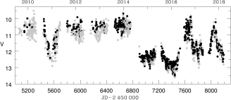
Figure 1: The light curve of RW Aur A+B in the $V$ band after 2010 based on the visual (the grey dots) and photoelectric (the black dots) data from the AAVSO database and our observations. The upper axis is for calendar years, the ticks correspond to the beginning of each year.

Recently RW Aur A has undergone two major dimming events with unprecedented parameters (Berdnikov et al., 2017). The first one has occurred in 2010–11 ($\Delta t\sim 150^{\rm d},$ $\Delta V\sim 2$ mag) and the second even deeper dimming started at 2014 summer and continues until now as shown in Fig. 1 and considered in more detail by Rodriguez et al. (2013); Rodriguez et al. (2016, 2018). Non-trivial behaviour of the star during these events was discussed by Antipin et al. (2015), Petrov et al. (2015), Schneider et al. (2015), Shenavrin, Petrov & Grankin (2015), Bozhinova et al. (2016), Facchini et al. (2016), Takami et al. (2016). Most of these authors agree that the dimming events were due to the eclipse of the star by a dust screen, but the nature of the screen is a matter of debates: a tidal arm between the components of the binary (Rodriguez et al., 2013), a dusty disc wind (Petrov et al., 2015; Bozhinova et al., 2016) or a warped inner disc (Facchini et al., 2016). Note that Takami et al. (2016) discussed (1) occultation by circumstellar material or by a companion and (2) changes in the mass accretion and concluded that neither scenario can simply explain all the observed trends.

Here we present results of our photometric and polarimetric observations of RW Aur A, carried out from 2010 to 2018, which, in our opinion, support the dusty wind model. Preliminary results of our campaign were presented by Lamzin et al. (2017). We will not discuss here the properties of RW Aur B, because we believe that it is a subject of a separate research. Average stellar magnitudes and polarization of the B component in different spectral bands are presented in Table 7 and are used here only to correct unresolved photometry and polarimetry of RW Aur A+B for the contribution of the B component as described in Appendix B.

In the following, we will accept that the distance to the binary is 163 pc (Gaia Collaboration et al., 2016, 2018; Luri et al., 2018) and inclination of RW Aur A disc axis to the line of sight $i$ is $60\degr$ as a compromise between the values $55\aas@@fstack{\circ}51\pm 0\aas@@fstack{\circ}13$ (Rodriguez et al., 2018) and $77^{+13}_{-15}$ deg. (Eisner et al., 2007).

The rest of the paper is organized as follows. In Section 2 we describe our observations and present their results in Section 3. Section 4 is devoted to the interpretation of the results in terms of a dusty disc wind model. Some parameters of the model (the dust temperature, the dusty wind mass-loss rate) are estimated in Section 5. We also state in this Section that relatively large errors in the coordinates of RW Aur A in the Gaia DR2 are caused by a variable contribution of the scattered light from the dusty wind. A brief summary of our main results is provided in the last section.

2 Observations

The spatially unresolved observations of RW Aur A+B in the optical bands were obtained at the Crimean Astrophysical Observatory (CrAO) from 2009 November to 2018 April. The measurements were carried out with the CrAO 1.25-m telescope (AZT-11) equipped with either the Finnish five-channel photometer or the FLI PL23042 CCD camera. The photomultiplier tube was used during the bright phases of the star $(V\sim 9$–$11$ mag) and the CCD detector for the fainter phases. All photometric observations were obtained in the $BVR_{\rm J}I_{\rm J}$ and sometimes in the $U$ filter. Differential photometry was performed on CCD images and absolute photometry from photomultiplier observations, with an accuracy not worse than 0.05 mag in all filters. Results of the CrAO optical observations are presented in Table 1, small part of which was published by Babina et al. (2013). Throughout the paper we will use ${\rm rJD}={\rm JD}-2\,450\,000$ instead of the Julian dates (JD).

Table 1: Unresolved optical photometry of RW Aur

rJD	$V$	$U-B$	$B-V$	$V-R_{\rm J}$	$V-I_{\rm J}$
7992.51	11.54	0.08	0.92	0.97	1.79
7998.54	11.25		0.96	1.02	1.93
7999.51	11.26	$-0.11$	0.85	0.97	1.86

Tables 1–6 are available in their entirety in a machine-readable form in the online journal. A portion is shown in the text for guidance regarding its form and content.

Resolved optical photometry of RW Aur A+B was performed from 2014 November to 2018 January with a 2.5-m telescope of the Caucasian Mountain Observatory (CMO) of Sternberg Astronomical Institute of Lomonosov Moscow State University (SAI MSU) equipped with a mosaic CCD camera based on two E2V CCD44-82 detectors (pixel size 15 µm) and a set of standard Bessel $UBVR_{\rm c}I_{\rm c}$ filters. Primary data processing (bias subtraction, flat field correction) was performed in a standard way. During our observations the seeing varied from about $0.7$ to $1.5$ arcsec, and we used the procedure described in Appendix A.1 to obtain resolved photometry of RW Aur components.

Differential photometry was performed relative to 1–5 comparison stars, taken from the list available from the AAVSO web page http://www.aavso.org (Kafka, 2018). Results of resolved photometry for the A component are presented in Table 2. The final photometric uncertainty given in Table 2, in most cases, determined by uncertainties in the magnitudes of the comparison stars.

Table 2: Resolved optical photometry of RW Aur

rJD	$U$	$\sigma_{U}$	$B$	$\sigma_{B}$	$V$	$\sigma_{V}$	$R_{\rm c}$	$\sigma_{R}$	$I_{\rm c}$	$\sigma_{I}$
7077.20			13.65	.02	12.98	.02	12.44	.05	11.69	.02
7376.42							14.92	.06
7986.53	13.26	.05	13.52	.02	12.78	.02	12.09	.05	11.17	.02

Unresolved near infrared (NIR) observations of RW Aur A+B were carried out between 2011 March and 2018 March with the $1.25$-m telescope of Crimean laboratory of SAI MSU equipped with a single-channel InSb-photometer in the standard $JHKLM$ photometric system. $J$ and $K$ magnitudes of the comparison star BS 1791 was adopted from the catalog of Johnson et al. (1966). There are no $H,$ $L$ and $M$ magnitudes of BS 1791 in the catalog, so we calculated them using expressions from Koornneef (1983) paper. The photometer and the methodology of observations are described by Shenavrin et al. (2011). The results of our observations are presented in Table 3, such as some portion of them are shown in figure 1 of Shenavrin et al. (2015) paper.

Table 3: Unresolved NIR photometry of RW Aur

rJD	$J$	$\sigma_{J}$	$H$	$\sigma_{H}$	$K$	$\sigma_{K}$	$L$	$\sigma_{L}$	$M$	$\sigma_{M}$
5625.30	8.56	.01	7.71	.01	6.86	.00	5.42	.01
5636.28	8.87	.01	7.95	.01	7.05	.01	5.59	.01
8007.50	8.64	.01	7.91	.01	7.03	.01	5.23	.01	4.50	.03

Another portion of NIR data were obtained between 2015 December and 2017 December in the $JHK$ bands of MKO photometric system at the 2.5-m telescope of CMO SAI MSU equipped with the infrared camera-spectrograph ASTRONIRCAM (Nadjip et al., 2017). During the NIR observations the seeing varied from about $1.0$ to $1.5$ arcsec, at the seeing worse than 1.5 arcsec unresolved photometry was performed. Differential photometry was performed relative to 1–5 comparison stars in the field of view, near-IR magnitudes of which are known from the 2MASS catalog. Results of resolved NIR observations are presented in Table 4.

Table 4: Resolved NIR photometry of RW Aur A

rJD	$J$	$\sigma_{J}$	$H$	$\sigma_{H}$	$K$	$\sigma_{K}$
7414.25	12.63	0.03	11.12	0.04	9.02	0.03
7418.24			11.10	0.05	9.04	0.03
7450.25	11.95	0.04	10.30	0.05

The $UBVR_{\rm J}I_{\rm J}$ polarimetry of the object during the first eclipse (2010–2011) has been secured using a five-colour double-beam single-channel photopolarimeter installed at the 1.25-m CrAO telescope (Piirola, 1988). The first observation was made on 2011 January 22 (${\rm rJD}=5584.45$), the last one – on 2012 March 12 (${\rm rJD}=5999.30$). As long as this instrument integrates radiation in a relatively large aperture ($10$ arcsec), a total polarization for both components was determined (see Table 5).

Table 5: Unresolved polarimetry of RW Aur.

rJD	Band	$p$	$\sigma_{p}$	PA	$\sigma_{\rm PA}$
		%	%	$\degr$	$\degr$
5592.29	$U$	9.204	0.384	43.98	1.19
	$B$	7.735	0.192	42.89	0.71
	$V$	6.608	0.243	45.68	1.05
	$R_{\rm J}$	6.308	0.075	45.82	0.34
	$I_{\rm J}$	6.252	0.095	46.43	0.44
5601.19	$U$	4.235	0.382	48.89	2.58
	$B$	4.505	0.197	47.41	1.26
	$V$	4.127	0.192	51.84	1.33
	$R_{\rm J}$	3.468	0.092	51.04	0.76
	$I_{\rm J}$	3.415	0.082	50.15	0.69

Col. 3–4: the polarization degree and its error.

In the second, deeper eclipse of 2014–2018 we have made polarimetric measurements of RW Aur in the $VR_{\rm c}I_{\rm c}$ bands with the SPeckle Polarimeter (SPP) of the 2.5-m telescope of SAI MSU. The SPP is an EMCCD-based double-beam polarimeter with a rotating half-wave plate (HWP). The optical scheme of the instrument forms on the detector two orthogonally polarized images of the object alongside. The HWP plays role of modulator, which allows to implement the method of double difference and measure both Stokes parameters characterising the linear polarization of the object. The demodulation was performed computationally post-factum. Safonov et al. (2017) described the instrument design and the method of polarimetry. Appendices A.2 and B contain some specifics of methodology related to separate measurements of the components of the relatively close binary. Results of polarimetry for the A component are presented in Table 6 and discussed in the next section.

Table 6: Resolved optical polarimetry of RW Aur A.

rJD	Band	$m$	$\sigma_{m}$	$p$	$\sigma_{p}$	PA	$\sigma_{\rm PA}$
				%	%	$\degr$	$\degr$
7318.6	$V$	14.35	0.15	20	2	39	2
8061.5	$I_{\rm c}$	9.8	0.2	5.56	0.1	42.9	0.1

Col. 1: Date of observation rJD; Col. 3–4: the magnitude and its error in the respective band; Col. 5–6: the polarization degree and its error.

3 Results

3.1 Photometry

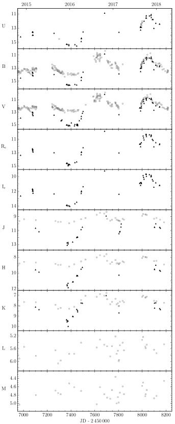
Figure 2: Light curves of RW Aur A$+$B in different spectral bands. The open squares denote the unresolved observations of RW Aur A+B and the black triangles represent the resolved observations of RW Aur A. The upper axis is for calendar years, the ticks correspond to the beginning of each year.

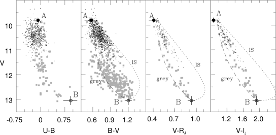
Figure 3: The colour–magnitude diagrams for RW Aur A+B based on the unresolved observations in the visual bands before (the black dotes) and after (the grey squares) 2010 September. The positions of the B component, found from the resolved photometry of the binary, are shown with the open circles. The filled black circle in each panel marks an estimated pre-eclipse position of the A component (see text for details). The dashed line is for the expected colour–magnitude track for RW Aur A+B assuming that the $V$ magnitude of the A component decreases down to 17 mag, such as the extinction does not depend on $\lambda.$ The dotted line is a similar curve, but for the standard extinction law $(R_{\rm V}=3.1).$

The light curves in the $UBVR_{\rm c}I_{\rm c}JHKLM$ bands covering the period from 2014 September to 2018 April are presented in Fig. 2. One can see from the figure that there is an interval ${\rm rJD}\approx 7350-7450$ of relatively constant brightness (‘plateau’), which is clearly seen in the $UBV$ bands and gradually disappears to the $K$ band, where the minimal brightness is reached when the plateau in the visual bands begins. It looks like the larger wavelength $\lambda,$ the earlier the star comes out from the eclipse. The light curves in the $L$ and $M$ bands look different and we will say more about this discussing Fig. 6.

Colour–magnitude diagrams for RW Aur A+B based on the unresolved photoelectric and CCD observations in $UBVR_{\rm J}I_{\rm J}$ bands carried out before and after 2010 are shown in Fig. 3. Results of our observations (Table 1) as well as data adopted from B. Herbst (Herbst et al., 1994), ROTOR (Grankin et al., 2007), and the AAVSO databases are used. It can be seen that as RW Aur A fades, the magnitudes and colour indices of RW Aur A+B tend to values corresponding to RW Aur B.

The dashed line in the figure shows the behaviour of the object under suggestion that the brightness of RW Aur A is attenuated equally in all bands (grey absorption), while the dotted one corresponds to the case when the absorption is accompanied by the standard (interstellar) reddening with $R_{\rm V}=3.1$ (Savage & Mathis, 1979). To construct these curves it was necessary to choose initial, i.e. not distorted by circumstellar absorption, stellar magnitudes of the A component in each band. These values are chosen so that the two curves are the envelopes of most observed points. The position of RW Aur A thus found is shown in each panel of Fig. 3 with the filled black circle.

Note that the presence of a hot (accretion) spot on the surface of the star leads to the fact that even in the absence of eclipses the magnitudes and colour indices of RW Aur A have to change both because of the variability of the accretion rate and the axial rotation of the star (Dodin, Lamzin & Sitnova, 2013). It means that the derived stellar magnitudes are pre-eclipse values averaged over time. The $U-B$ colour index additionally changes because of the variable contribution of emission lines in the $U$ and $B$ bands (Petrov et al., 2001). Due to this reason the pre-eclipse position of RW Aur A in the diagram $V$ versus $U-B$ is shown only for illustrative purposes and the $U$ magnitude will not be used hereinafter. According to our estimations the uncertainty of the derived $B$ magnitude is $\approx 0.2$ and that of the $VRI$ magnitudes is $\approx 0.1.$

We remind that before the first deep eclipse in 2010 Petrov & Kozack (2007) had concluded that ‘the brightness and colour variations are due primarily to absorption in dust clouds formed by the disc wind’. In the frame of this hypothesis, the fact that observed points on the Fig. 3 are located to the left of the curve with $R_{\rm V}=3.1$ means that the absorbing dust should be on average larger than the interstellar dust. A similar conclusion was reached by Schneider et al. (2015) and Günther et al. (2018) from the comparison of RW Aur A’s X-ray spectrum before and during the eclipse. However, we will demonstrate in Sect. 4.1 that there is an alternative interpretation of the colour–magnitude diagrams as well as the X-ray data.

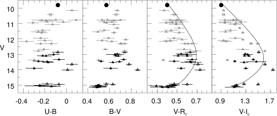
Figure 4: The colour–magnitude diagrams for RW Aur A in the visual bands. The triangles correspond to the different periods of our resolved observations: the ingress to the most deep dimming of the star (2014 November – 2016 February, filled black), the egress from the deep dimming (2016 February – April, open black), irregular dimmings of smaller amplitude (2016 September – 2018 January, grey). The open squares represent observations by White & Ghez (2001) carried out before 2010. The black circles mark the pre-eclipse positions of the star derived from Fig. 3. The solid curve in the two right-hand panels represent the model, which fits the polarimetric and photometric data obtained between 2011 January and 2016 April – see equations  (1–3) in Section 4.1.

Colour–magnitude diagrams of RW Aur A based on our resolved observations in the $UBVR_{\rm c}I_{\rm c}$ bands (Table 2) are presented in Fig. 4. UX Ori (UXOR) type behaviour [‘bluing effect’, see e.g. Grinin (1988) and references therein] is clearly seen in the $V-R_{\rm c},$ $V-I_{\rm c}$ colours and possibly present in the $B-V$ colour. It is reasonable to assume that explanations of the effect in both cases are similar: as the star fades, the contribution of more blue light, scattered by the circumstellar dust, increases (Grinin, 1988). However, the amplitude $(\Delta V\approx 5$ mag) and duration (several years) of RW Aur A’s dimmings are significantly larger than in the case of UXORs, which indicates that in our case, we dealing with suggestive of a larger scale phenomenon than an eclipse of the star by a relatively small dust cloud orbiting the star.

Note also that in contrast to UXORs the bluing effect is absent in the $U-B$ colour and marginally present in the $B-V$ colour (two left-hand panels of Fig. 4). Possibly it is due to the dominant and large contribution of the so-called broad components of the emission lines in the $U$ and $B$ bands, respectively [see Petrov et al. (2001) and figure 1 in Facchini et al. (2016)]. These lines apparently originated far enough from the star (Petrov et al., 2001), so eclipses of the star and the line formation region occur in different ways. This fact deserves a separate discussion that is beyond the scope of this paper.

One more nontrivial feature of RW Aur A is the difference of all colour indices at the ingress to the deepest eclipse (the minimal magnitude $V=15.1$ was observed on 2016 January 2 and 2016 March 9, rJD=7390.41 and 7457.19, respectively) and at the egress from it. As far as we know, this behaviour has not been observed in UXORs. A possible explanation of this feature will be discussed in Section 4.2.

Figure 5: The relationship between the $V$ and NIR magnitudes of RW Aur A. Open triangles correspond to our resolved observations during 2014–2018 eclipses and black filled triangles correspond to the unresolved observations of RW Aur A+B before 2010, corrected for an average contribution of RW Aur B (see text for the references). The position of RW Aur B (the black circle) is shown for comparison.

From 2015 to 2018 we succeeded to carry out simultaneous resolved photometry of the binary in the visual and NIR bands during only 7 nights. In order to compare the behaviour of the star in visual and NIR bands, we plot the $V$ versus $K$ dependence in the left panel of Fig. 5 using these observations. Data of unresolved simultaneous observations of RW Aur A+B in the $V$ and $K$ bands carried out before 2010 (Rydgren, Strom & Strom, 1976, 1982; Rydgren & Vrba, 1981, 1983), and corrected for an average contribution of RW Aur B (Table 7) are also plotted in the panel. It can be seen that the $V$ and $K$ magnitudes of RW Aur A are well correlated. The correlation is broken only in the initial phase of the egress from the most deep eclipse, when the star was still on the plateau stage in the $V$ band, while the eclipse in the $K$ band was over (see Fig. 2). The point falling from a linear dependence in the left panel of Fig. 5 corresponds just to this period.

It can be seen from the middle and right panels of Fig. 5 that the $J,$ $H$ and $K$ magnitudes of RW Aur A are also proportional to each other, so that points observed before and during the eclipses form a continuous (quasi-linear) sequence. (The designations and the data sources are the same as for the left panel).

Figure 6: The relationship between the $K,$ $L$ and $M$ magnitudes of RW Aur A+B based on the unresolved observations of the binary. The open squares are for our data acquired during 2010–2011 and 2014–2018 eclipses, the black squares are for our observations between eclipses (2011–2014) and data from the literature before 2010 (see text for references). The position of RW Aur B (the black circle) is shown for comparison, according to the data from Table 7 and Appendix C.

The situation is more interesting at larger wavelengths $(\lambda\gtrsim 2.5$ µm). Due to the absence of resolved photometry of the binary in the $L$ and $M$ bands, we plot in Fig. 6 $K$ versus $L$ and $K$ versus $M$ dependencies for RW Aur A+B. Our observations during 2010–2011 and 2014–2018 eclipses are shown with the open squares and our observations between the eclipses (2011–2014) as well as observations before 2010 (Mendoza V., 1966; Glass & Penston, 1974; Rydgren, Strom & Strom, 1976, 1982; Rydgren & Vrba, 1981, 1983) are shown with the black squares. It is clearly seen that the data acquired during the eclipses and before or between them form two separate sequences in the $K$ versus $L$ panel: at the same brightness in the $K$ band the binary is systematically more bright in the $L$ band during the eclipses.

Probably, there are also two branches in the $K$ versus $M$ dependence for RW Aur A+B (the right-hand panel of the figure), but we cannot state this with any certainty, since have at our disposal only three simultaneous out-of-eclipse observations in the $K$ and $M$ band. We note only that the $M$ magnitude of the binary is almost independent on its $K$ magnitude during the eclipses.

Fig. 6 describes the total behaviour of both components, but we believe that the above-mentioned features characterize the behaviour of RW Aur A. Otherwise it is difficult (if at all possible) to understand why these features are so closely connected with the eclipses. Besides that the relative contribution of the B companion to the total flux in the $L$ and $M$ bands is $<20$ per cent (see the position of the B component in the panels of Fig. 6 and Appendix C).

Figure 7: The colour–magnitude diagrams in the NIR bands for RW Aur A (two left-hand panels) and the binary RW Aur A+B (two right-hand panels). The open symbols (the triangles for the A component and the squares for the binary) correspond to our observations during the eclipses. Observations carried out before 2010 and out of eclipses (2011–2014) are shown with the black filled symbols: the squares in the right-hand panels represent the unresolved observations of the binary and the triangles in the left-hand panels are for the unresolved observations of RW Aur A+B, corrected for the contribution of the B component. The position of RW Aur B is shown by the black circle.

NIR colour–magnitude diagrams $K$ versus $J-K$ and $H-K$ of RW Aur A are presented in the two left-hand panels of Fig. 7. It can be seen that during the eclipses the larger $K$ magnitude of the star the more ‘red’ its $J-K$ and $H-K$ colours.

Due to the absence of resolved observations of the binary in the $L$ and $M$ bands we presented $K$ versus $K-L$ and $L-M$ colour–magnitude diagrams for RW Aur A+B rather than RW Aur A (see two right-hand panels of Fig. 7). As in the left-hand panels of the figure, the open and filled black symbols correspond to the observations during the eclipses and out of them, respectively. One can see that when the brightness of the binary in the $K$ band tends to that of the B component, the $K-L$ and $L-M$ colour indices of RW Aur A+B tend to the values, which correspond to much more ‘red’ (cold) radiation than the radiation of RW Aur B.

To characterize the colour behaviour of this radiation, it is necessary to see how the $L-M$ colour index varies depending on the $L$ or $M$ rather than $K$ magnitude as shown in Fig. 7. It follows from the respective colour–magnitude diagram (see Fig. 8) that there is no correlation between the $M$ magnitude of the binary and its $L-M$ colour index during the eclipses.

As before (in the discussion of the $K$ versus $L,$ $M$ diagrams), we believe that the $M$ versus $L-M$ dependence for the binary reflects the behaviour of RW Aur A.

Figure 8: The colour–magnitude diagram $M$ versus $L-M$ of RW Aur A+B based on the unresolved observations of the binary. The open squares are for our observations during the eclipses 2010–2011 and 2014–2018, the black squares are for our data acquired between the eclipses and the data before 2010 taken from the literature (see text for references). The black circle marks the position of RW Aur B as derived in Appendix C.

3.2 Polarimetry

Before the onset of the eclipses period (before 2010) the polarization of RW Aur A+B was measured by several authors. The earliest polarimetric record, which we found in the literature, was made by Bastien (1982) on 1977 February 22 using a single-channel PMT-based polarimeter. Similar instrumentation was used by Hough et al. (1981); Schulte-Ladbeck (1983); Bastien (1985). Bastien (1982) and Bastien (1985) used custom filters with bands resembling $V,$ $R,$ $I$ of the Johnson system. Hough et al. (1981) and Schulte-Ladbeck (1983) used the Johnson $V,$ $R,$ $I$ bands. We did not transformed observations to the Cousins system as long as it is not necessary at our level of precision.

For the epochs of these observations we used the photometric data published in these papers or found the $V$ band (unresolved) photometry in the AAVSO database spaced by no more than 1 day from the polarimetry epoch.

The mentioned authors measured the total polarization of the binary. Using the method described in Appendix B, we reduced both photometry and polarimetry for the contribution of RW Aur B, and thus obtained an approximate estimate of the polarization and brightness of RW Aur A. The results are presented in Fig. 9 as crosses.

In 2003 the continuum polarization of RW Aur A was measured by Vink et al. (2005) using the ISIS spectrograph on the 4.2-m William Hershel Telescope. Their results are also plotted in Fig. 9 with crosses.

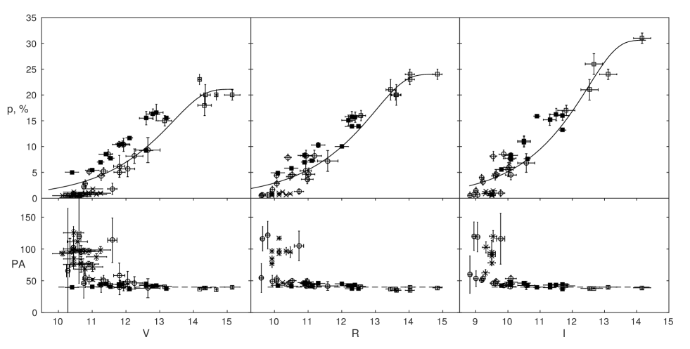
Figure 9: The polarization degree (the upper row) and PA (the lower row) for RW Aur A as function of its magnitude in the $V$, $R$ and $I$ bands (from left to right). The crosses correspond to the measurements by Bastien (1982); Hough et al. (1981); Schulte-Ladbeck (1983); Bastien (1985); Vink et al. (2005) corrected for the B component contribution (a period before eclipses). The open circles are for our unresolved polarimetry and photometry in 2011–2012 corrected for the B component (within and soon after the first eclipse). The open squares are for the resolved observations from 2015 October to 2016 April, the filled squares are for the same, but from 2016 October to 2018 April (both datasets correspond to the second eclipse). The solid lines show the approximation by equations (1–3) of the data obtained from 2011 January to 2016 April (rJD=5584.45 – 7496.20). The dashed lines in the lower panels indicate the direction normal to the jet axis (Dougados et al., 2000).

One can see from the figure that the star showed significant polarization variability during the pre-eclipse period. The fraction of polarization $p$ varied between 0.1 and 1.5 per cent, and the polarization angle (PA) was between $50\degr$ and $130\degr.$ The large relative polarization variability gives an additional support to the suggestion that the interstellar polarization of the object is negligible in comparison to an enormous intrinsic polarization observed in the eclipses. There is no correlation between the brightness and $p$ or PA during the pre-eclipse period.

Our unresolved polarimetric observations was started in the beginning of 2011, during the first eclipse, and ended in 2012, after the return of the object to normal brightness. They were also corrected for the contribution of the B component and plotted in Fig. 9. At that period the polarization degree increased by several times up to 5–7 per cent and PA changed to $30\degr-50\degr.$ The PA roughly coincided with the direction perpendicular to the jet axis. The anti-correlation between the polarization and brightness was observed as for UXORs (Grinin, 1994). After return to the normal brightness the polarization also returned to the pre-eclipse level.

Results of the resolved polarimetry obtained with the SPP are plotted in Fig. 9. The amplitude of variability in $p$ increased in the second eclipse (the observations from 2015 October to 2018 April). The maximum observed polarization amounted to 30 per cent in $I_{\rm c}.$ But remarkably, the character of the $p$–mag dependence is consistent for both eclipses as well as the colour–magnitude diagrams from Section 3.1. We employ this fact and will interpret the corresponding data jointly in Section 4.1.

It is worth noting that the range of variability of PA is reduced even more in the second eclipse while remaining centered on the direction perpendicular to the jet axis: PA$=38\degr-42\degr$.

After the deepest part of the second eclipse, starting from autumn 2016 (see Figs. 1, 2), a similar $p$–mag dependence is observed. However, as one can see in Fig. 9, the overall dependence shifted upwards (or leftwards) in all bands with respect to the data obtained before and during the deepest eclipse (summer 2014 – summer 2016). In other words, a polarization typical for a certain brightness of the object increased. In the meantime the orientation of polarization was consistently perpendicular to the jet axis, even while the stellar flux almost returned to the pre-eclipse level.

In some aspects (e.g. bluing effect, strong anticorrelation between the brightness and polarization degree), the behaviour of RW Aur A resembles UXOR-type variability. This supports the hypothesis that irregular eclipses are caused by circumstellar dust. On the other hand, RW Aur A shows a much longer duration and amplitude of eclipses and a much larger polarization than a typical UXOR (Grinin et al., 1991; Yudin, 2000). Also, in contrast to RW Aur A, UXORs usually demonstrate significant variability of PA during the eclipse, which is caused by chaotic changes in an illumination pattern and visibility of a protoplanetary disc (Oudmaijer et al., 2001).

4 Interpretation

4.1 Polarimetric and colour variability

The analysis of polarimetric and photometric variability of UXOR variables shows that in all cases it agrees well with the hypothesis, which states that all polarization is produced by scattering on a circumstellar dust (Bastien, 1987; Grinin, 1994). The alternative hypothesis, where the polarization is due to dichroic extinction by aligned circumstellar dust grains, has not been reliably confirmed.

In the case of RW Aur A, even if there is some polarized flux produced through dichroic absorption, it nevertheless cannot explain all polarization. Indeed, as was noted above, the observed ‘bluing effect’ indicates that there is a significant contribution of radiation scattered by the dust in the total flux of the star. Obviously, this radiation should be polarized. In other words, the polarized flux of RW Aur A could be some mixture of polarization by aligned dust and polarization due to scattering, but the second mechanism dominates.

For a simple check of this suggestion we remind the following features of polarization behaviour of the object during the eclipses. First, PA does not vary with brightness of the object. Second, PA was the same in both deep eclipses. Third, PA almost coincides in the $V$, $R_{\rm c}$ and $I_{\rm c}$ bands. These features force us to believe that if there is some polarization by absorption, the corresponding dust particles should be aligned normally to the disc plane for a prolonged period of time.

We cannot exclude such possibility, but a firm conclusion would require additional data on the spatial distribution of polarized flux around the object. The corresponding analysis is outside the scope of the current work. For the moment, we will assume that all polarization of RW Aur A is generated by scattering.

The fact that PA coincides with the position angle of the major axis of the on-sky projection of the disc with precision of $3\degr-5\degr$ allows to draw the following conclusions on the scattering environment:

1. Such orientation of polarization is not expected for a protoplanetary disc (Whitney & Hartmann, 1993). Instead, it can be explained if the circumstellar dust is extended in the direction of the rotational axis of the disc.

2. The high degree of alignment between the disc and PA requires an axial symmetry for the circumstellar dust arrangement. The brightness variability is connected with changes in the optical thickness not in the azimuthal direction, but along the rotational axis of the disc.

3. The stability of PA gives evidence for the relative persistency of this symmetrical dusty circumstellar environment.

Thus, the polarization is likely to be produced by scattering on a persistent dust cloud occupying the region above the protoplanetary disc and possessing axial symmetry around the rotation axis of the disc. Similar geometries were considered by Whitney & Hartmann (1993), but on much larger scales (ca. 500 au) and in the context of infalling envelopes.

In our case the typical extent of the dust cloud is much smaller as long it is not resolved. Apart from this, in the case of RW Aur A spectral observations (Petrov et al., 2015; Bozhinova et al., 2016; Facchini et al., 2016) and a relatively old age of the object favour an outflow rather than an infall of matter. Thus, we conclude that the polarization of RW Aur A is generated by scattering in a dusty wind, which also causes eclipses.

As we noted above, the pre-eclipse irregular variability of RW Aur before 2010 is also interpreted as irregular eclipses by ‘dust clouds formed by the disc wind’ (Petrov & Kozack, 2007). But that variability had a much shorter timescale and a much smaller amplitude [see Berdnikov et al. (2017) and references therein for details]. We suppose that before 2010 relatively small gas-dust clouds were ejected sporadically at different azimuths of the disc and only some of them eclipse the star. It probably explains the absence of $p$–mag and PA–mag correlations before 2010 – see above and Schulte-Ladbeck (1983). Such dust clouds casted shadows on the disc randomly, and as long as the disc generated most of polarized flux then, this gave rise to large variations in PA. We believe that due to some reasons during the eclipses 2010–2011, 2014–2018 the outflow became axisymmetric and, as a consequence, deep long eclipses started and a scattering dusty cone developed above the disc. As a result PA changed by $90\degr$ and the polarization degree rose.

Fig. 10 illustrates the assumed geometry of the gas-dust outflow responsible for the eclipses. Due to some reason dust from the protoplanetary disc of RW Aur A is being risen by the disc wind and crosses the line of sight to the star in the region Ia. The variations of the density of the dust causes a variable extinction. Dust rises to the region Ib. This region by definition is a part of the wind, where a characteristic optical thickness in the wind is more than unity. Its brightness depends on illumination conditions. After passage of the region Ib dust rises further to the less dense region II of the wind, which is not screened from the star by the lower region of the wind. The region II accumulates the dust coming from the disc and smoothes short-term variability of the dust mass-loss rate in the lower region of the wind. Due to these two factors it appears relatively stable to an observer, unlike the regions Ia and Ib.

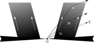
Figure 10: A cartoon depicting a section of the protoplanetary disc with the dusty disc wind. The region of the wind responsible for the absorption of the direct stellar radiation is denoted by Ia. The slightly higher region Ib is the part of the wind, which is affected by the self-absorption. The brightness of this region varies in time due to change in illumination conditions caused in turn by fluctuations in the dust mass-loss rate. In the same time the upper region II due to its large size smoothes the variability of the dust mass-loss rate and is illuminated by the star relatively constantly. Thanks to both these factors the region II appears as an unvarying source. The thin lines are for some paths, along which stellar light reaches the observer (direction OE).

We consider the simplest model of the object in order to interpret in a quantitative way the observed $p$–mag and colour–mag dependencies observed in the period of the eclipses. In this model the star with its circumstellar environment, which has an optical thickness depending on the altitude above the disc, is replaced with three sources of radiation. The first of them corresponds to the star, it is characterized by the flux $F_{*}$. The flux $F_{*}$ decreases during eclipse due to absorption by circumstellar dust (region Ia), but this absorption does not induce polarization (see above). The second source is a region of the wind with a significant optical thickness (region Ib in Fig. 10). The flux $F_{\rm vw}$ from this source changes in time primarily due to change in conditions of illumination by the star and probably due to absorption of already scattered radiation by the wind. We will call this source as the ‘variable region of the wind’, or simply ‘variable wind’. Note that changing reflection nebulae around stars are common, e.g. Hubble’s variable nebula (Lightfoot, 1989).

The third source corresponds to a significantly more extended region of the wind with a low optical thickness (the region II in Fig. 10). We assume that during the deepest eclipse it is illuminated by the star permanently and always visible to the observer. Therefore the total flux $F_{\rm cw}$ from this ‘constant region of the wind’ (hereafter constant wind) does not change in time during considered period of the eclipse. However, we emphasize that on longer timescales this part of the wind is also variable, e.g. it did not existed at all during the pre-eclipse period.

Now we consider how the observed $VR_{\rm c}I_{\rm c}$ fluxes and polarization of these sources vary with optical thickness $\tau_{*,V},$ characterizing fading of the stellar radiation in the $V$ band. For the initial brightness not affected by circumstellar extinction we adopt the pre-eclipse stellar magnitudes $m_{*,V}=9.8$, $m_{*,R}=9.4$, $m_{*,I}=8.9$ found in Section 3.1. The flux of the constant wind is estimated from the magnitudes $m_{{\rm cw},V}=15.2$, $m_{{\rm cw},R}=14.8$, $m_{{\rm cw},I}=14.3$ observed at the bottom of the deepest eclipse (see Fig. 2 and Table 2). As for the variable wind, we assume that its non-eclipsed magnitude is greater than the magnitude of the constant wind by $\Delta m_{\rm cw}$ in all three bands.

The fluxes not affected by the absorption $F_{*,i},$ $F_{{\rm vw},i},$ $F_{{\rm cw},i}$ $(i=V,R_{\rm c},I_{\rm c})$ are related to the corresponding stellar magnitudes:

$$2.5\log_{10}{\left({F_{{\rm cw},i}\over F_{*,i}}\right)} =m_{*,i}-m_{{\rm cw},i},$$

$$2.5\log_{10}{\left({F_{{\rm vw},i}\over F_{{\rm cw},i}}\right)} =\Delta m_{\rm cw}.$$ (1)

In the following we assume that the optical thickness in the direction to the star in the $R_{\rm c}$ and $I_{\rm c}$ bands differs from the same value in the $V$ band by $\zeta_{R}$ and $\zeta_{I}$ times. The dimming of the variable wind is characterised by its ‘effective’ optical thickness: $F_{\rm vw}=F_{{\rm vw},i}{\rm e}^{-\tau_{\rm vw}}$. We note that this takes into account both variation in conditions of wind illumination and self-screening of the wind from the observer. It seems reasonable to assume that the fading of the star and the variable wind are interrelated. Specifically, we assume that the optical thicknesses of the variable wind $\tau_{\rm vw}$ and in the direction to the star $\tau_{*}$ are related: $\xi=\tau_{\rm vw}/\tau_{*}$, where the coefficient $\xi$ is constant in time and across the $VR_{\rm c}I_{\rm c}$ bands. For the sake of simplicity the fraction of polarization $p_{{\rm vw},i}$ $(i=V,R_{\rm c},I_{\rm c})$ is considered to be equal for the constant and variable regions of the wind.

Under all these assumptions it is possible to write three pairs of relations for the total flux and polarization of the object:

$$F_{i}(\tau_{*})=F_{*,i}\,{\rm e}^{-\tau_{*}\zeta_{i}}+F_{{\rm vw},i}\,{\rm e}^{-\tau_{*}\zeta_{i}\xi}+F_{{\rm cw},i},$$ (2)

$$p_{i}(\tau_{*})=p_{{\rm vw},i}\,{F_{{\rm vw},i}\,{\rm e}^{-\tau_{*}\zeta_{i}\xi}+F_{{\rm cw},i}\over F_{i}},$$ (3)

where $i=V,$ $R_{\rm c},$ $I_{\rm c},$ and $\zeta_{V}=1$ by definition.

This model should reproduce not only the observed $p$–mag dependence (Fig. 9), but also the $V$ versus $V-R_{\rm c},$ $V-I_{\rm c}$ dependencies (Fig. 4). However it does not seem rational to use all available observations, because, as noted before in Section 3.2, after 2016 September scattering by the circumstellar environment increased so dramatically that significant polarization was observed even when the star almost returned to the pre-eclipse brightness. Due to this reason, to determine the model parameters, we employ only photometry and polarimetry obtained between 2011 January and 2016 April.

The model parameters have been found by orthogonal least squares fitting of the data with equations (1–3) in $p$–mag space. The minimum residual is achieved at the following parameter values: $\xi=0.32\pm 0.02,$ $\Delta m_{\rm cw}=2.66\pm 0.03,$ $\zeta_{R}=0.88\pm 0.01,$ $\zeta_{I}=0.71\pm 0.01,$ $p_{{\rm vw},V}=21.1\pm 0.4,$ $p_{{\rm vw},R}=24.0\pm 0.4,$ $p_{{\rm vw},I}=30.6\pm 0.4.$ Note that for the determination of these parameters we used more than 150 individual measurements, so the model is not expected to overfit the observations.

The corresponding curves are plotted in Fig. 9 and two right-hand panels of Fig. 4. The fact that the modelled curve in Fig. 9 describes well observations before 2016 September and not so well after this moment can be explained by the aforementioned increase in scattering by the circumstellar dust. Due to the same reason colour indices measured after 2016 September are bluer than the modelled ones. Note that the data points in the colour–magnitude diagram obtained between 2014 November and 2016 April are fitted by the model quite well. In the next section we will discuss how the constructed model could be adjusted in order to explain different colours of the object during ingress and egress in this period.

Judging by $\Delta m_{\rm cw}$ value the contribution of scattered radiation in the total observed flux is quite significant. Even at maximum brightness (at $\tau_{*}=0$ in our model) the fraction $\eta$ of scattered radiation in all bands amounts to $\approx 10$ per cent, which follows from the relation $(i=V,R_{\rm c},I_{\rm c})$

$$\eta_{i}={F_{{\rm vw},i}+F_{{\rm cw},i}\over F_{*,i}+F_{{\rm vw},i}+F_{{\rm cw},i}}$$ (4)

taking into account equations (1). The contribution of scattered radiation rises with fading RW Aur A: at $V\approx 13$ it approaches approximately 50 per cent. At brightness minimum the flux is dominated by scattered light, which leads to emergence of the plateau in the light curve and in the $p$–mag dependence. It is worth noting that the flux from the circumstellar dust decreases with fading the star. When the object reaches the plateau in the light curve, the flux from region Ib decreases by $\approx 10$ times compared to the initial $(\tau_{*}=0)$ level.

We conclude, therefore, that polarimetric and photometric variability of RW Aur A can be explained by the modified UX Ori model: variable star + variable circumstellar environment.

It seems quite reasonable that optical thickness decreases ($\zeta_{I}<\zeta_{R}<\zeta_{V}=1),$ and polarization degree rises $(p_{{\rm vw},V}<p_{{\rm vw},R}<p_{{\rm vw},I})$ as wavelengths increases (Draine, 2003). However it would be premature to make any conclusions on dust properties on the basis of these results due to simplicity of the model. In this respect, we note that the conclusion about the prevalence of large dust grains in the absorbing shell does not undoubtedly follows neither from our colour–magnitude diagram of RW Aur A$+$B (Fig. 3) nor from X-ray data of Schneider et al. (2015) or Günther et al. (2018) because it was made without accounting for scattered light.

At first, at initial stages of the eclipses RW Aur A definitely becomes redder, as can be seen from the colour–magnitude diagrams $V$ versus $V-R_{\rm c},$ $V-I_{\rm c}$ in Fig. 4 as well as $K$ versus $J-K$ and $H-K$ diagrams in Fig. 7. It means that during the eclipses circumstellar absorption is selective rather than neutral up to the $K$ band, i.e. $\sim 2$ µm. What is more, the observed colour–magnitude tracks of the binary in Fig. 3 well can be shifted to the left relative to the theoretical tracks, corresponding to the interstellar (IS) reddening law, due to the ‘bluing effect’ of the primary, so it is not obvious that the extinction law of the circumstellar dust really differ from the IS one.

The conclusion of Schneider et al. (2015) and Günther et al. (2018) on the prevalence of micron size grains is based on a very large discrepancy between observed dimming of the star $\Delta V$ at the moments of X-ray observations and estimated extinction of RW Aur A’s light $A_{\rm v}$ found from the convertation of derived hydrogen column densities $N_{\rm H}$ to extinction $A_{\rm v},$ using the relationship between them, which corresponds to the IS medium. In particular, Günther et al. (2018) found that 2017 January 9 (rJD=7763) $A_{\rm v}\approx 200\pm 50,$ while the observed brightness of RW Aur A decreased at that moment by $<3$ mag in comparison with average value before 2010.

But $A_{\rm v}$ found from the X-ray observations characterizes the extinction in the direction to the star, the radiation of which can be indeed strongly attenuated, while the observed emission in the optical band is a much less absorbed scattered light from the region Ib and II of the dusty wind (see the next subsection for a quantitative estimation). We conclude therefore that it is prematurely to state that large dust grains dominate in the absorbing region.

4.2 On some features of RW Aur A’s light curve

Within the scope of the suggested interpretation, the observed variability of RW Aur A after 2010 is caused by variations in the intensity of the dusty wind. Now we consider in detail the period between 2015 August and 2016 April covering the deepest eclipse when the object reached $V\approx 15$ mag. As we noted before, for this eclipse the ingress is two times longer than the egress. The second feature of this eclipse is bluer colours in the visible range during the ingress than during the egress. For example, on 2015 October 20 (rJD = 7316) and 2016 April 17 (rJD = 7496) the object brightness in the $V$ band was almost the same: 14.2 and 14.0, respectively. In the meantime colour indices $V-R_{\rm c}$ and $V-I_{\rm{}_{c}}$ on these dates differ by 0.3 and 0.6, respectively.

It is possible to qualitatively explain such behaviour, if the fading of the variable wind starts somewhat later than the eclipse of the star. Within the framework of dusty wind hypothesis such situation is possible, if the variable wind is located above the line of sight to the star, which is in agreement with the smaller optical thickness for the variable wind than for the obscuring one in our simple model. In this case the variable wind would be still visible during the ingress and would add blue radiation to the total flux. On the other hand, during the egress the star would become visible before the variable wind starts to brighten. Because the former is still reddened by circumstellar extinction, the object should look more red than at the ingress.

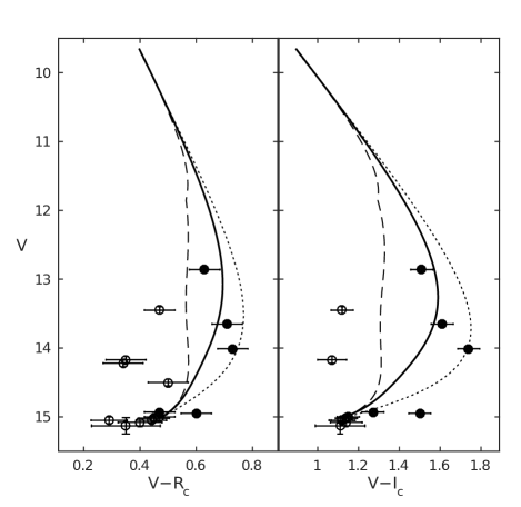
Figure 11: The colour–magnitude diagrams $V-R_{\rm c}$ and $V-I_{\rm c}$ versus $V$ for RW Aur A for the deepest eclipse (2015 August – 2016 April). The open circles are for the ingress, the filled circles are for the egress. The solid line corresponds to the model described by equations (1–3). The dashed and dotted lines are for the model, which takes into account a delay between the eclipse of the star and the fading of the variable wind, see equations (5) and (6).

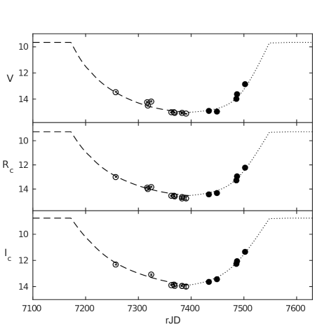
Figure 12: The light curve for the deepest eclipse (2015 August – 2016 April). The open circles represent the ingress, the filled circles are for the egress. The dashed and dotted lines represent the model with a delay between the eclipse of the star and the fading of the variable wind, see equations (5) and (6).

In order to quantitatively describe these features of object’s behaviour, we used the model from the previous section with several additional assumptions. First, the optical thickness for the star $\tau_{*}$ in the course of the ingress rises linearly with time and then decreases also linearly with the same rate. Second, the optical thickness for the variable wind $\tau_{\rm vw}$ changes in time according to the same law, but with smaller amplitude and shifted in time. Therefore, four parameters are added: the moment of eclipse centre $t_{\rm c}$, the duration of the ingress (which is equal to the duration of the egress) $t_{\rm e}$, the time delay of variable wind’s eclipse $\Delta t_{\rm e}$, and the maximum optical thickness along the direction to the star $\tau_{*,{\rm e}}$.

In the frame of this model the optical thicknesses for the star and the variable wind depend on time in the following way:

$$\tau_{*}(t)=\left\{\begin{array}[]{lrl}0,&&\!\!\!\!\!t\leq t_{\rm c}-t_{\rm e},\\ \tau_{*,\rm e}(t-t_{\rm c}+t_{\rm e})/t_{\rm e},&t_{\rm c}-t_{\rm e}<&\!\!\!\!\!t\leq t_{\rm c},\\ \tau_{*,\rm e}(t_{\rm c}+t_{\rm e}-t)/t_{\rm e},&t_{\rm c}<&\!\!\!\!\!t\leq t_{\rm c}+t_{\rm e},\\ 0,&t_{\rm c}+t_{\rm e}<&\!\!\!\!\!t,\\ \end{array}\right.$$ (5)

$$\tau_{{\rm vw}}(t)=\xi\tau_{*}(t-\Delta t_{\rm e}).$$ (6)

By the substitution of $\tau_{*}(t)$ and $\tau_{\rm{vw}}(t)$ into equations (2) and (3) we obtained light curves and colour–magnitude diagrams. We used them in fitting the $VR_{\rm c}I_{\rm c}$ light curves and the colour–magnitude diagrams $V$ versus $V-R_{\rm c},$ $V-I_{\rm c},$ corresponding to the period between 2015 August and 2016 April. The following values of the parameters were found: $t_{\rm c}=7360$ rJD (corresponds to 2015 December 3), $t_{\rm e}=190$ days, $\Delta t_{\rm e}=40$ days, $\tau_{*,{\rm e}}=15$. As can be seen from Figs. 11 and 12, this simple model describes both the prolonged ingress and the bluer colour in that period reasonably well.

Note the large value of optical depth in the direction to the star $\tau_{*,{\rm e}},$ which corresponds to the IS-like extinction with $N_{\rm H}\sim 3\times 10^{22}$ cm${}^{-2},$ which is close to the value found by Schneider et al. (2015) from the X-ray observations in 2015 April 16 (rJD = 7129).

RW Aur A looks much more bright than one can expect from $\tau_{*,{\rm e}}$ value due to the dominant contribution of light scattered by the dust wind. This also complies with basic geometric considerations. The wind is axially symmetric, i.e. occupies $2\pi$ radians in azimuthal direction. On the other hand it is extended above the disk at least up to line of sight that connects the star to the observer ($30^{\circ}$ from the disk midplane) where is causes deep and long eclipses. Therefore the solid angle of the wind observed from the star should be $\Omega>2\pi\cos i\approx\pi$. The wind intercepts (absorbs and scatters) more than $\approx 1/4$ of stellar radiation.

Unfortunately, the model cannot be used for fitting the NIR observations due to the lack of polarimetric observations in this band and unaccounted contribution from the accretion disc (see Appendix C).

In this regard, we note the following episode. On ${\rm rJD}=7774.4$ the brightness of RW Aur A+B in the $M$ band has reached the historical maximum of $m_{M}=4.36\pm 0.02,$ but after 11 days only the flux in this band decreased by 1.8 times (Table 3). This episode corresponds to the descending branch of the visible light curve (see Fig. 2), but soon after that the brightness of the star started to increase. Also from ${\rm rJD}=7804$ till 7823 the brightness of RW Aur A in the $J$ band increased by $1.4$ mag (Table 4). Realistic model of the dusty wind should reproduce such succession of events.

5 Dusty disc wind model

5.1 On the dust temperature in the disc wind

Shenavrin et al. (2015) have found that at the beginning of 2014 eclipse (${\rm rJD}>6700$) the observed flux of RW Aur A+B in the $L$ and $M$ bands (3–5 µm) increased. The authors attributed the excess emission to radiation of a hot dust at the temperature of about 1000 K. To consider this statement in more detail, we have compared the pre-eclipse SED of RW Aur A (see Appendix C) with the SED of the star in the eclipse phase.

Unfortunately we did not succeed to obtain both spatially resolved data in the $B$–$K$ bands and unresolved data in the $LM$ bands during the same night. Observations carried out on 2015 December 28 (rJD $\approx 7385.4$), when RW Aur A was at the ‘plateau phase’ (see Fig. 2), are almost satisfy this condition. Resolved photometry of the star in the $BVR_{\rm c}I_{\rm c}$ bands was obtained 3 days before and 5 days later this date, but brightness of the star in these bands did not differ within errors of measurements: $V=15.08\pm 0.05$ and $15.13\pm 0.02,$ respectively. These data are shown in Fig. 13 with filled triangles.

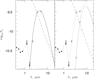
Figure 13: The approximation of RW Aur A’s SED at the epoch of minimal brightness (${\rm rJD}=7385.4$) by theoretical models without (the left-hand panel) and with (the right-hand panel) subtraction of the pre-eclipse fluxes in the L and M bands. The observed fluxes of the star (in units erg s^-1 cm^-2 µm${}^{-1}),$ found from the spatially resolved observations, are shown with the filled triangles. The open squares represent results of the unresolved observations of RW Aur A+B corrected for the (average) contribution of RW Aur B. The upper limits to the flux in the $J$ and $H$ bands were found as discribed in the text. The circles in the right-hand panel are data in the $LM$ bands corrected additionally for the pre-eclipse stellar contribution of RW Aur A. The pre-eclipse SED of the star is shown with the dashed line. The grey solid curves are the blackbody curves for $T_{{\rm d}}=670$ K (the left-hand panel) and $T_{{\rm d}}=350$ K (the right-hand panel). The dotted curve in both panels is the expected SED of the star, which ‘by definition’ coincides with the blackbody curve in the left-hand panel.

Fluxes of RW Aur A in the $KLM$ bands at rJD=7385.4 (open squares in Fig. 13) are found by subtracting average fluxes of RW Aur B from the respective fluxes of the binary. However, the fluxes of RW Aur A+B in the $J$ and $H$ bands are less than the respective average fluxes of RW Aur B. Due to this reason, we derived upper limits of the fluxes in these bands subtracting from the summary flux the minimal flux of the B component found from the total period of its observations.

It is clearly seen from Fig. 13 that the observed SED of the star is double-peaked. As far as the polarization of light in the $VR_{c}I_{c}$ bands at the moment of interest was very large, we believe that the observed radiation at $\lambda<2$ µm is a radiation of the star and its disc scattered to the Earth by the extended semi-transparent part of the wind (the region II in Fig. 10). We suppose that observed flux at longer wavelengths is connected with the thermal emission of the dust wind (the region Ia+Ib or some its part in Fig. 10).

To characterize this radiation, we can relate all observed radiation in the L and M bands to the dust wind. In fact, this case has been considered by Shenavrin et al. (2015) and corresponds to the optically thick dusty environment, which absorbs all radiation of the star and its accretion disc at least shortward $\lambda=5$ µm and re-radiates it at $\lambda\gtrsim 3$ µm. Then its spectrum is the Planck curve, which passes throughout the observed fluxes in the L and M bands. In our case the corresponding temperature is $T_{{\rm d}}=670$ K (the grey solid curve in the left-hand panel of Fig. 13).

This case is not a completely unreasonable, because radiation in the $K$ band is definitely absorbed by the circumstellar dust, as discussed below. Indeed, as it is shown in Appendix C, contributions of the accreting star and the disc to the observed flux in the $K$ band before 2010 were approximately equal. Therefore, if radiation of the star and a half of the disc is completely absorbed by the circumstellar dust, then the $K$ magnitude of RW Aur A must have decreased by $\approx 1.5$ mag, i.e. down to $\approx 8.3\pm 0.13$ mag. But at ${\rm rJD}=7376.38$ (i.e. 9 days before the date for which we consider the SED), it was $9.98\pm 0.05,$ which means that almost all disc emission was absorbed.

We may suppose that the star and the inner disc contribute to the $L$ and $M$ bands. To understand how it modifies our estimate of $T_{\rm d},$ we consider another limiting case, in which we subtract the pre-eclipe fluxes from the observed ones. This case may correspond either to the optically thin at $\lambda>3$ µm dusty environment, or to the case, where the optically thick (at $\lambda>3$ µm) part of the region Ia is located so close to the disc that it does not screen the central source. As before, we assume for simplicity that the radiation shortward 3 µm is a blackbody radiation. Then, using the two obtained points (the circles in the right-hand panel of Fig. 13), we derive $T_{\rm d}=350$ K. In the optically thin case the physical dust temperature should be even less, because the dust absorption cross-section decreases with the wavelength and due to Kirchhoff’s law the emissivity is also reduced, it makes the colour temperature of the dust radiation higher than the physical dust temperature.

We restrict ourselves to the statement that $T_{{\rm d}}<670$ K, because in fact $T_{{\rm d}}$ was found from the comparison of the observed and blackbody $L-M$ colour indices only, whereas in reality the dusty wind is semi-transparent for radiation in the 3–5 µm band and cannot be considered as a single temperature blackbody. One can hope to develop a model of the thermal structure of the wind from the analysis of spectra of RW Aur A in the 2–10 µm band. Note that the model has to explain the absence of the correlation between the brightness of the star in the $M$ band and the $L-M$ colour index (see Fig. 8).

5.2 Mass-loss rate of the wind

We estimate now the mass-loss rate of the dust wind, using some very general assumptions about the geometry of the wind: the wind is launched from the disc plane at radii $R_{1}<r<R_{2}$ and has a velocity $\bf V_{\rm p}$ inclined at an angle $\alpha$ to the disc plane (see the upper panel of Fig. 14). The AC segment in the panel is perpendicular to the streamlines ${\bf V_{\rm p}}.$ The surface $W$ formed by rotation of the AC segment around the $z$-axis is a truncated cone. Its area is

$$S_{\rm AC}={\rm\pi}\Delta R\,{\sin}^{2}\alpha\left({{2R_{1}\cos\gamma}\over{\sin\beta}}+\Delta R\,\sin\alpha\right),$$ (7)

where $\Delta R=\left(R_{2}-R_{1}\right),$ $\gamma={\rm\pi}/2-i<\alpha,$ $\beta=\alpha-\gamma.$ Then

$$S_{\rm AC}>2{\rm\pi}R_{1}\cos\gamma\sin\alpha\,{{\Delta R\,\sin\alpha}\over{\sin\beta}}=2{\rm\pi}R_{1}l\cos\gamma\sin\alpha,$$ (8)

where $l$ is the length of the segment AB, which is the part of the line of sight (inside the wind) connecting the star and the observer.

To estimate the mass-loss rate, we need to employ some additional assumptions on the wind density and velocity. We will adopt that the density $\rho_{\rm w}$ is constant on each surface parallel to the $W$ surface inside the region occupied by the wind. In the meantime, in each streamline $\rho_{\rm w}$ decreases with height above the disc. Finally, the velocity is assumed to be constant in the flow, at least above the AC segment along the flow.

Now one can find a lower limit of the mass-loss rate through the disc wind as follows

$$\dot{M}_{\rm w}=\rho_{\rm w}^{\rm A}V_{\rm p}\,S_{\rm AC}>2{\rm\pi}R_{1}\cos\gamma\sin\alpha\,V_{\rm p}\,l\rho_{\rm w}^{\rm A}.$$ (9)

A gas particle density $n_{\rm H}$ is related to a gas density of the wind at the point A via the relation $\rho_{\rm w}^{\rm A}=\mu m_{\rm u}n_{\rm H}^{\rm A}$, where $m_{\rm u}\approx 1.7\times 10^{-24}$ g is the atomic mass unit and $\mu\approx 2$ is the molecular weight of the gas, which predominantly consists of molecular hydrogen due to the low gas temperature. Schneider et al. (2015) have found from X-ray observations that the absorbing column density $N_{\rm H}\approx 2\times 10^{22}$ cm^-2 in the dim state of RW Aur A (rJD = 7129), and probably was larger at the minimal brightness eight months later (${\rm rJD}=7385.4$). Note that $N_{\rm H}=\int n_{\rm H}{\rm d}l<ln_{\rm H}^{\rm A},$ because wind’s gas density decreases along the streamlines with the distance from the disc.

Günther et al. (2018) have found a much larger value of $N_{\rm H}=(4\pm 1)\times 10^{23}$ cm^-2 from the X-ray observations carried out in 2017 January, but noted that more inner (dust-free) regions of the outflow can contribute significantly to the hydrogen column density they found. Note in this connection that our simple model of the dust wind, corresponding to the period of RW Aur A’s minimal brightness (see Section 4.2), predicts the value of $N_{\rm H},$ which is very close to the value found by Schneider et al. (2015) and that is why we used this value to estimate $\dot{M}_{\rm w}.$

Taking into account that $V_{\rm t}=V_{\rm p}\sin\beta$ , where $V_{\rm t}$ is the transverse component of disc’s wind velocity (see the upper panel of Fig. 14), one can find that

$$\dot{M}_{\rm w}>2{\rm\pi}\mu m_{u}R_{1}V_{\rm t}N_{\rm H}{\tan\alpha\over{\tan\alpha-\tan\gamma}}>2{\rm\pi}\mu m_{u}R_{1}V_{\rm t}N_{\rm H}.$$ (10)

It is not possible to estimate transverse velocity $V_{\rm t}$ from our model of photometric variability described in Section 4.2, where we found how optical depth of the wind $\tau_{\rm vw}$ varied with time at some period of the eclipse, because we do not know how $\tau_{\rm vw}$ varied with the height above the disc. Due to this reason we will adopt low limit $V_{\rm t}\approx 1$ km s^-1 found by Rodriguez et al. (2018).

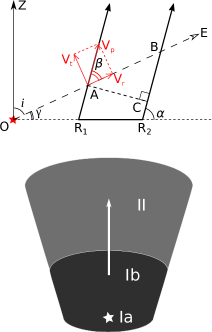
Figure 14: Schematic representation of the dusty wind: the cross section (the upper panel) and the on-sky projection (the lower panel). The region of the wind, in which radiation of RW Aur A shortward $\approx 2$ µm is absorbed predominantly $(\tau_{*}>1$ along the line of sight), is shown in the lower panel (not to scale) in dark grey, and the scattering region $(\tau_{*}<1)$ in light grey. The position of the star and the axis of its jet (the blue lobe) are shown in white colour.

Finally, to estimate $\dot{M}_{\rm w}$, we need only the inner radius $R_{1}$ of the disc wind formation region. Decreasing of the observed flux in the $K$ band means that radiation of the wind in this band is negligible (see also Section 5.1). Therefore, the wind formation region should be further from the central star than the part of the accretion disc, which radiated in the $K$ band before 2010, i.e. further than 0.1 au according to Eisner et al. (2014).

Substituting $V_{\rm t}>1$ km s^-1 and $R_{1}>0.1$ au in equation (10) we found that the mass-loss rate of the dusty disc wind is $\dot{M}_{\rm w}>10^{-9}\,{\rm M_{\odot}}$ yr${}^{-1}.$ One can compare this very conservative lower limit with the mass-loss rate $\dot{M}_{\rm jet}\approx 2\times 10^{-9}\,{\rm M_{\odot}}$ yr${}^{-1},$ found by Melnikov et al. (2009) in the blue jet of RW Aur A (the magnetospheric collimated wind) and with the accretion rate on to the star $\dot{M}_{{\rm acc}}\approx 1.1\times 10^{-7}\,{\rm M_{\odot}}$ yr^-1 (see Appendix C).

The optical depth of the wind along the line of sight OE (see the upper panel of Fig. 14) is proportional to $N_{\rm H}.$ Then it follows from equation (10) that dimming of RW Aur A can occur not only due to variations of the mass-loss rate $\dot{M}_{\rm w},$ but also due to variability of the inclination of the wind streamlines to the disc plane.

5.3 The scattering dust and the relative position of RW Aur’s components in the sky

The existence of a significant scattering dusty environment should affect results of precise astrometric observations of RW Aur A, because in the frame of the dusty wind model the position of the photocentre of the star + circumstellar environment system does not coincide with that of the star. Specifically, one can expect that as RW Aur A fades the photocentre of the system shifts along the axis of the blue lobe of the jet away from the star (see the lower panel of Fig. 14). Due to this reason the observed distance $r$ and the position angle $\theta$ of RW Aur B is expected to differ from the same values observed when the circumstellar environment is absent by

$$\Delta r=-\Delta s\cos\left(\theta_{0}-\theta_{\rm jet}\right)=+3.6\,\Delta l\,\,\frac{D,\,{\rm pc}}{163},\quad{\rm mas}$$ (11)

$$\Delta\theta={\Delta s\over r_{0}}\sin\left(\theta_{0}-\theta_{\rm jet}\right)=+0\aas@@fstack{\circ}20\,\Delta l\,\,\frac{D,\,{\rm pc}}{163}$$ (12)

where $\Delta s$ is the angular shift of the photocentre; $\Delta l$ is the linear shift in au, corresponding to $\Delta s$; $D\approx 163$ pc is the distance to RW Aur A; $\theta_{\rm jet}=130\degr$ is the position angle of the blue jet (Dougados et al., 2000), and $r_{0}\approx 1.45$ arcsec, $\theta_{0}\approx 256\degr$ are the ‘real’ separation and the position angle of the B component relative to the primary, respectively (Bisikalo et al., 2012). It follows from equations (11–12) that due to the presence of the scattering circumstellar environment the observed distance and the position angle must be larger than the ‘real’ ones.

The $\Delta s$ value can be found from the model of the dusty disc wind, which takes into account radiative transfer effects in a proper way. In order to get an approximate value of $\Delta s,$ we estimate the projection of the optically thick part of the dust wind to the sky (the black region in the lower panel of Fig. 14). One can very crudely estimate the projected area $S_{\rm d}$ of this region using relation between observed flux $F_{\lambda}$ and the Planck function $B_{\lambda}=B_{\lambda}(T_{{\rm d}},\lambda)$

$$F_{\lambda}={B_{\lambda}S_{\rm d}\over D^{2}}$$ (13)

at $\lambda=5$ µm. Here $D$ is the distance to RW Aur and $T_{{\rm d}}$ is the dust temperature, which is certainly $<670$ K (see Section 5.1) Thus, we found that $S_{\rm d}\gtrsim 2\times 10^{26}$ cm².

A very preliminary estimation of the projection size of the ‘absorbing’ part of the wind can be obtained as $\sqrt{S_{\rm d}},$ which is $\gtrsim 1$ au. As follows from the lower panel of Fig. 14 the projection of the ‘scattering’ part of the wind has larger extension than the ‘absorbing’ part, so one can expect that the photocentre of the system star + scattering circumstellar environment is shifted relative to the star by $\Delta l\gtrsim 1$ au during the deep eclipse.

Our $I_{\rm c}$-band CCD images provide the most accurate relative astrometry of the binary components among the observations, which we have at our disposal. Nevertheless, their accuracy is not enough to detect the shift of the photocentre. For example, when the $I_{\rm c}$ magnitude of RW Aur A changed from $12.27\pm 0.02$ (rJD=7486.2) to $9.99\pm 0.10$ (rJD=8073.4) the projected distances $r$ between the components ($1493\pm 5$ and $1495\pm 8$ mas, respectively) as well as the position angle $\theta$ ($254\aas@@fstack{\circ}27\pm 0\aas@@fstack{\circ}04$ and $254\aas@@fstack{\circ}08\pm 0\aas@@fstack{\circ}07,$ respectively) remained the same within the errors.

The accuracy of Gaia astrometric data is much better: according to Gaia Data Release 2 (the epoch 2015.5) $r=1488.64\pm 0.92$ mas, $\theta=254\aas@@fstack{\circ}468\pm 0\aas@@fstack{\circ}025$ (Gaia Collaboration et al., 2018). The Gaia DR2 catalog contains results averaged over many individual observations, so it would be very interesting to consider whether $r$ and $\theta$ values depend on the brightness of RW Aur A. It is possible that relatively large errors in the coordinates of RW Aur A in the Gaia DR2 (an order of magnitude larger than that of RW Aur B) is caused by a variable contribution of the scattered light from the dusty wind.

Concluding remarks

We found from photometric and polarimetric observations of the visual young binary RW Aur that:

1. The colour and magnitude variations of RW Aur A+B in the $UBVRIJHK$ bands occur mainly due to variability of RW Aur A.

2. As the brightness decreases, the colour indices and magnitudes of the binary in the bands from $U$ to $K$ tend to values corresponding to RW Aur B, but in the $LM$ bands they tend to a more bright and red (cold) state.

3. The colour indices $V-R_{\rm c}$ and $V-I_{\rm c}$ of RW Aur A increase initially with decreasing its brightness, indicating that the extinction is selective rather than neutral, but then begin to decrease (the bluing effect).

4. As the brightness decreases, the radiation of RW Aur A becomes strongly polarized (up to 30 per cent in the $I_{\rm c}$ band).

5. Since 2015 and up to 2018 April the polarization vector is directed perpendicular to the jet.

In some aspects (the bluing effect, the strong anticorrelation between the brightness and the polarization degree) the behaviour of RW Aur A is similar to UXORs, confirming the hypothesis that the fading of the star is due to obscuration by circumstellar dust. However, there are principal differences between UXORs and the RW Aur A case, namely, a much longer duration and a larger depth of eclipses, higher linear polarization and stability of its orientation during the eclipses. This indicates that if in the case of UXORs the eclipses are produced by relatively small clouds of circumstellar dust (Grinin, 1988), then in the case of RW Aur A the eclipses are caused by a much more extended circumstellar dusty environment.

We have developed simple models to explain the observations. These models and observational evidences suggest the following about the nature and the parameters of the dusty environment associated with RW Aur A:

1. The circumstellar dust not only selectively absorbs, but also selectively scatters light of the central star, re-emitting in total more than a quarter of its radiation. For example, after 2014 the contribution of the scattered radiation to the $V$ band even in the bright state is $\sim 10$ per cent.

2. As the brightness of RW Aur A decreases, the relative contribution of the scattered light increases and exceeds 50 per cent at $V\gtrsim 13$ mag. However, along with a decrease in the intensity of the stellar light, the absolute intensity of the scattered light also decreases, the flux from the circumstellar dust weakens by a factor of $\sim 10$ at the deepest eclipse. It can be a consequence of both a self-absorption in the dusty environment and changes in the conditions of illumination of the environment by the star.

3. The geometry of the dusty environment possesses axial symmetry with respect to RW Aur A’s jet axis. Irregular variations in the brightness of RW Aur A are due to inhomogeneities, moving along the rotational axis of the disc rather than in the azimuthal direction.

4. The environment is a dusty wind, which is launched from the disc regions with radii $>0.1$ au. The dust temperature is about several hundred K, and the mass-loss rate was $>10^{-9}$ M_⊙ yr^-1 at the period of minimal brightness of RW Aur A.

To give a quantitative interpretation of the observations and to estimate the parameters of the dusty wind, we have used very simple models. A more realistic approach should take into account the radiative transfer for a broad spectral region and changes in the dust properties with distance from the disc plane. However, only photometric and integral polarimetric data are not enough to develop such a model.

Important information about the most opaque wind regions may be obtained from IR spectra of RW Aur A between 2 and 20 µm taken in the faint state. An analysis of spectral lines at shorter wavelengths will allow to probe more hot regions of the magnetospheric and disc wind. In this connection, it would be interesting to obtain new spectral observations of the jet with a high angular resolution similar to those performed by Dougados et al. (2000) and Woitas et al. (2002) before 2010.

One can hope to obtain some information about the scattering region of the wind by analysing variations in the relative position of the A and B components as a function of the brightness of the A component, using the Gaia data. It would be interesting to study the spatial distribution of polarized radiation in visible bands. In addition, the detection and study of polarization in NIR bands could provide useful information about the dust properties.

As long as in the case of RW Aur A we are witnessing the onset of dust entrainment by the disc wind, the object provides a valuable opportunity to study related processes in dynamics.

We finally note that we agree with Petrov & Kozack (2007) that the dusty wind had been blowing before the start of the large-scale eclipse in 2010, but then the dust clouds were comparatively small and almost did not screen the disc. The question about the causes of the wind enhancement remains open. Most likely, this is associated with a restructuring of RW Aur A’s disc due to the close fly-by of RW Aur B, but why the intensity of the dusty wind has increased in $\approx 350$ years after enhancing the accretion rate and launching the jet (Berdnikov et al., 2017) is unclear.

Appendix A Binary separation technique

A.1 Binary separation in the case of photometric observations

The CCD image of the binary can be presented as a sum

$$Y(x,y)=a_{1}\Psi(x-x_{1},y-y_{1})+a_{2}\Psi(x-x_{2},y-y_{2}),$$ (14)

where $\Psi(x,y)$ is the point spread function (PSF), which is assumed to be the same for both stars. In the case of photometric measurements we use a few nearby bright stars as PSF models. The coefficients $a_{1}$, $a_{2}$ and the coordinates $x_{1},$ $y_{1},$ $x_{2},$ and $y_{2},$ as well as the corresponding uncertainties are determined by least-squares fitting the model $Y$ to the observed image. In our case of a relatively bright object, the uncertainties in the coefficients are small, so the final uncertainties in stellar magnitudes are determined in the most cases by uncertainties in magnitudes of comparison stars.

A.2 Binary separation in the case of polarimetric observations

In the case of polarimetric observations with the SPP, the separation technique described above cannot be applied because, due to the small field of view, there are no stars, which can be taken as a PSF model. However, even in this case it is possible to separate the stars. In order to do this, we first rotate the image in a such way that the main axis of the system becomes horizontal (see Fig. 15-a).

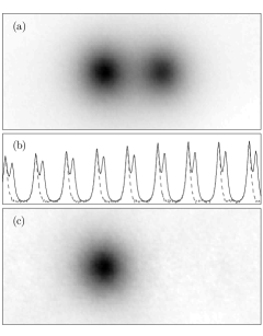
Figure 15: Binary separation technique. (a) the original rotated image. (b) a part of the one-dimensional representation of the image $u_{k}$ (the black line) along the pixel index $k.$ The dashed line is for the solution of equation (15) with parameters, at which the function $S$ reaches the minimum. (c) the two-dimensional representation of the solution.

Then the two-dimensional image, represented as a pixel matrix $F_{ij}$ ($i=1,N_{x}$; $j=1,N_{y}$), can be reshaped into a column vector $\bf u$ with elements $u_{k}$ ($k=1,N_{x}N_{y}$) which are shown in Fig. 15-b with the solid line. We suppose that the PSFs $\Psi(x,y)$ for both stars are equal and in a discrete form are represented as a matrix $\Psi_{ij}$ with the same size as $F_{ij},$ $\bf p$ (with elements $p_{k}$) is the corresponding one-dimensional representation of $\Psi_{ij}$. Then the vector $\bf u$ can be modelled as

$${\bf u}=(q\textbf{{M}}+\textbf{{I}}){\bf p},$$ (15)

where I is the identity matrix, copying the one-dimensional PSF $\bf p$ into itself; $\textbf{{M}}(\Delta)$ is a matrix, which spatially shifts $\bf p$ by $\Delta$ using linear or cubic interpolation; $q$ is the flux ratio of the components. Solving the equation (15) at a given $\Delta$ and $q$, we obtain the one-dimensional PSF $\bf p.$ However, the separation $\Delta$ and the flux ratio $q$ are not known, while the equation (15) can be solved at any $\Delta$ and $q.$ Numerical experiments with artificial observations with known parameters $q=q_{0}$ and $\Delta=\Delta_{0}$ show that if $\Delta\neq\Delta_{0}$ or $q\neq q_{0},$ then the solution $\bf p$ turns to be an oscillating and sign-variable function, and the amplitude of the oscillations increases with increasing deviations from the true values. Since negative $p_{k}$ are unphysical, the true parameters $\Delta$ and $q$ can be obtained by searching for the most positive solution $\bf p.$ To do this, we minimize the function

$$S(\Delta,q)=\sum\limits_{k}e^{-\frac{p_{k}}{\sigma}},$$ (16)

in which statistically significant negative values of $p_{k}$ give a much larger contribution than positive ones. $\sigma$ is the noise estimate for the obtained solution, which, in our case, can be calculated as $\sigma^{2}=0.5\sum_{k}(p_{k}-p_{k-1})^{2}/(K-1),$ where the summation is taken over pixels, which lay outside (on some adjustable criterion) the main peak of the two-dimensional representation of p, K is the number of terms in the sum. The one- and two-dimensional representations of the obtained solution are shown in Fig. 15(b, c).

The described method has been applied only to Stokes $I$-images, because they have a high signal-to-noise ratio. In the case of Stokes $Q$ and $U$ images we used PSF found from the respective $I$-image, assuming that PSFs in polarized and direct light are the same.

Appendix B Polarimetry of components of RW Aur

Polarimetry of RW Aur has been performed at the SPP using the method described by Safonov et al. (2017). The basic product of the method is a set of images of the object in the Stokes $I,$ $Q,$ $U.$ Examples are given in Fig. 16. The typical FWHM in these images is comparable with the distance between the components of the binary. Therefore, simple aperture photometry turns out to be inapplicable: the polarization of the brighter component may affect the measurement of the fainter one. In order to overcome this obstacle, we employed the method described in Section A.2 and estimated dimensionless Stokes parameters for both components of the binary. For the A component the Stokes parameters were converted to the fraction and angle of polarization, which are plotted in Fig. 9.

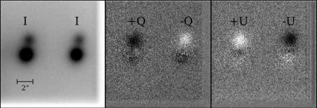
Figure 16: Images of RW Aur in the Stokes $I,Q,U$ (from left to right) obtained on 2015 October 28 (rJD=7324.37) in the $V$ band. The image of the binary is repeated twice, because the instrument is a two-beam polarimeter. The field of view is rectangular, its size is $5\times 10$ arcsec. RW Aur A is located above RW Aur B, and one can see that it dominates the polarized flux, while it is more faint in direct light.

The magnitude has been estimated on the basis of flux ratio and total magnitudes of the object obtained either from our photometry or from the AAVSO database for the respective dates. In the absence of simultaneous photometry, we use RW Aur B as a comparison star. As follows from our resolved photometry, RW Aur B is an irregular variable. Therefore, we will assume that the magnitude of the star is known with a certain additional error (see Table 7). These data along with the polarimetric data allow us to estimate the Stokes parameters $I,$ $Q,$ $U$ in flux units, which are also presented in the table.

Assuming that the character of RW Aur B variability has not changed significantly in the last 30 years, we can estimate the magnitude and the polarization of the A component from measurements of the total flux and the total polarization of the system

$$I_{A}=I_{T}-I_{B},\,\,\,\,Q_{A}=Q_{T}-Q_{B},\,\,\,\,U_{A}=U_{T}-U_{B}.$$ (17)

Here the Stokes parameters are in flux units, the subscripts $T,A,B$ denote a relationship to the system, the A component, and the B component, respectively.

Table 7: Average properties of RW Aur B.

band	$m$	$\sigma_{m}$	$I$	$\sigma_{I}$	$Q$	$\sigma_{Q}$	$U$	$\sigma_{U}$
			mJy	mJy	mJy	mJy	mJy	mJy
$U$	15.16	0.32
$B$	14.32	0.33
$V$	13.07	0.27	23	4	$-0.06$	0.05	$-0.22$	0.08
$R_{\rm c}$	12.17	0.25	38	6	$-0.12$	0.06	$-0.43$	0.09
$I_{\rm c}$	11.15	0.24	63	10	$-0.14$	0.09	$-0.86$	0.15
$J$	9.85	0.17
$H$	9.11	0.09
$K$	8.65	0.09

Col. 2–3: magnitude and its $1\sigma$ scatter due to variability; Col. 3–8: the Stokes parameters (in the equatorial reference system) and their errors.

Appendix C Pre-eclipse SED of RW Aur A and parameters of the star

As far as we know that the brightnesses of the binary components have been measured separately only twice before 2010 (White & Ghez, 2001; McCabe et al., 2006). This is clearly not enough to determine the spectral energy distribution (SED) of RW Aur A in the pre-eclipse state, bearing in mind its significant variability. We solved the problem as follows.

First, we constructed the time-averaged SED of RW Aur B, assuming that before and after 2015 it was the same. The stellar magnitudes in the 0.4–25 µm spectral band were taken from our resolved photometry in the $BVR_{\rm c}I_{\rm c}JHK$ bands and supplemented by observations from McCabe et al. (2006) in the $N$ ($\lambda_{{\rm eff}}=10.8,$ $\Delta\lambda=5.15$ µm) and $IHW18$ ($\lambda_{{\rm eff}}=18.1,$ $\Delta\lambda=1.6$ µm) bands. Applying the expression $\log_{10}F_{\lambda}=\log_{10}F_{\lambda}^{0}-0.4\,m_{\lambda}$ the stellar magnitudes were converted to the fluxes $F_{\lambda}$ (erg s^-1 cm^-2 µm${}^{-1})$ adopting $F_{\lambda}^{0}$ values from Bessell et al. (1998), McCabe et al. (2006). By means of spline interpolation of these data (the grey triangles and the dash-dotted line in Fig. 17) we estimated the brightness of the star in the $L$ and $M$ bands: $L_{\rm B}=8.05,$ $M_{\rm B}=7.70$ (the grey circles in the figure).

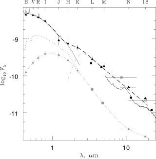
Figure 17: The observed and theoretical SED of RW Aur A and B. The triangles represent data from ground-based observations of the A (black) and B (grey) components. The black squares represent results of unresolved space (AKARI, WISE) observations of RW Aur, from which the contribution of RW Aur B is subtracted. The spline-approximation of the observed points is shown by the black dashed curve. The solid black curve is for the Spitzer spectrum. The grey solid and dotted curves are theoretical spectra for RW Aur A: the ‘star+accretion spot’ (the solid line) and the star only (the dotted line). The grey dashed line represents the SED of RW Aur A’s disc. See text for details. The filter $IHW18$ is denoted as ‘18’ in the figure. The flux is in erg s^-1 cm^-2 µm^-1 units.

To construct the SED of RW Aur A not distorted by a circumstellar dust extinction, we used the pre-eclipse stellar magnitudes of the star in the visual bands (see Section 3.1 and the filled black circles in Fig. 3). As far as pre-eclipse circumstellar extinction decreases with wavelength (see Petrov & Kozack (2007) and Section 3.1) it looks reasonable to assume that observed variability of RW Aur A+B longward $\approx 1$ µm is due to physical reasons rather than variable extinction. Based on this, we derived the pre-eclipse NIR magnitudes of the star by subtracting the contribution of the B component from averaged unresolved $JHK$ observations of RW Aur A+B before 2010 (Glass & Penston, 1974; Mendoza V., 1966; Rydgren, Strom & Strom, 1976, 1982; Rydgren & Vrba, 1981, 1983; Woitas, Leinert & Köhler, 2001). The same was done for the $L$ and $M$ bands, but interpolated rather than observed fluxes of the B component were subtracted. We also plot in Fig. 17 the results of resolved observations in the $N$ and $IHW18$ bands obtained by McCabe et al. (2006). All data mentioned in this paragraph are shown in the figure with black triangles. Results of unresolved space observations of the binary corrected for the contribution of the B component are also plotted in the figure in black: photometric data from AKARI (Ishihara et al., 2010, the open squares) and WISE (Wright et al., 2010, the filled squares) as well as spectral observations from Spitzer (Furlan et al., 2011, the solid black curve).

We reconstruct the SED of RW Aur A as follows. The observed spectrum of the star is strongly veiled, so it is difficult to derive its spectral type: values from K4 to K0 can be found in the literature (e.g. Petrov et al., 2001; Herczeg & Hillenbrand, 2014), which correspond to $4400$–$5100$ K range of effective temperatures $T_{{\rm eff}}$ (Herczeg & Hillenbrand, 2014). The spectral flux density ${\cal F}_{\lambda}^{*}$ for a stellar atmosphere with a compromise value of $T_{{\rm eff}}\approx 4750$ K and $\log_{10}g=4.0$ was calculated by using the ATLAS9 code (Kurucz, 1970; Sbordone et al., 2004).

To account for the observed veiling, it is necessary to add to the stellar radiation an emission from the accretion shock, the spectrum of which depends on the pre-shock gas velocity $V_{0}$ and particle density $N_{0}$ or $\rho_{0}\approx 2.1\times 10^{-24}(g)\times N_{0},$ assuming that the accreting gas as well as the stellar atmosphere have the solar elemental abundance.

It is reasonable to set $V_{0}=400$ km s${}^{-1},$ because an extension of an absorption feature in the red wing of some strong emission lines, e.g. He i $\lambda$5876 Å, in all observed spectra of RW Aur has just this value (e.g. Petrov et al., 2001; Alencar et al., 2005; Takami et al., 2016). Dodin & Lamzin (2012), Dodin et al. (2013) have found that $12.0\leqslant\log_{10}N_{0}<13.0$ in the case of CTTSs with strongly veiled spectra, so we adopted $\log_{10}N_{0}=12.5$ for RW Aur A. Then we calculated the spectral flux density ${\cal F}_{\lambda}^{{\rm acc}}$ emitted by the accretion shock with these values of $V_{0}$ and $N_{0}$ (Dodin, 2018).

As far as the geometry of RW Aur A’s accretion zone is unknown, we use a flux ${\cal F}_{\lambda}$ to construct the SED [as e.g. Calvet & Gullbring (1998) did] instead of the integration of the specific intensity of the stellar and accretion shock radiations over respective regions of the stellar surface. If the accretion shock occupies fraction $f$ of RW Aur A’s surface, then the observed flux is

$$F_{\lambda}={R_{*}^{2}\over D^{2}}\,\left[{\cal F}_{\lambda}^{*}\left(1-f\right)+{\cal F}_{\lambda}^{{\rm acc}}f\right]\equiv{R_{*}^{2}\over D^{2}}\,{\cal F}_{\lambda},$$ (18)

where $R_{*}$ is the stellar radius and $D$ is the distance to RW Aur.

To take into account an interstellar extinction we artificially reddened the flux ${\cal F}_{\lambda}$ using the standard $(R_{\rm V}=3.1)$ extinction curve (Bless & Savage, 1972), assuming that $A_{\rm V}=0.3$ (Petrov et al., 2001). As far as emission lines are important contributors in the $U$ band (see Section 3.1), we compare the resulting SED with observations longward 0.4 µm only.

Combining ${\cal F}_{\lambda}$ with $F_{\lambda}$ in Fig. 17 at $\lambda=0.55$ µm and varying $f$ parameter to fit the observed spectrum, we found from equation (18) that $f\approx 0.25$ and $R_{*}\approx 1.9$ $R_{\odot},$ in agreement with the lower limit of $1.3$–$1.5$ $\left(D,pc/140\right)$ $R_{\odot}$ found by Petrov et al. (2001). It can be seen from the figure that the resulting theoretical spectrum (the grey solid curve) is in a reasonable agreement with the average pre-eclipse SED of RW Aur A in the visible range. The corresponding spectrum of the star is shown in the figure for comparison (the grey dotted curve). We also calculated an expected veiling of RW Aur A in the $V$ band and found that it is $\approx 3,$ which coincides with the average value found by Petrov et al. (2001) from the pre-eclipse spectral monitoring of RW Aur.

Then the ‘formal’ bolometric luminosity of the star is $L=4{\rm\pi}R_{*}^{2}\sigma T_{{\rm eff}}^{4}\approx 1.6\,{\rm L_{\odot}}.$ The accretion rate is $\dot{M}_{{\rm acc}}=4{\rm\pi}R_{*}^{2}\,f\,\rho_{0}V_{0}\approx 1.1\times 10^{-7}\,{\rm M_{\odot}}$ yr^-1 and the accretion luminosity (without the disc contribution) is $L_{{\rm acc}}=0.5\,\dot{M}_{{\rm acc}}V_{0}^{2}\approx 1.4\,{\rm L_{\odot}},$ so the total luminosity of the accreting star is $L_{*}\approx 1.6\,{\rm L_{\odot}}+1.4\,{\rm L_{\odot}}=3.0\,{\rm L_{\odot}}.$

The pre-eclipse SED longward the $M$ band, i.e at $\lambda>5$ µm, is not very accurate due to insufficient observational data. We approximated it by a straight line with the slope ${\rm d}\left(\log_{10}F_{\lambda}\right)/{\rm d}\left(\log_{10}\lambda\right)\approx-5/3.$ Observed values $F_{\lambda}$ deviate from this line not more than 30 per cent, which is enough for our goals. A spline-approximation of RW Aur A’ SED in the 0.4–25 µm band is shown in Fig. 17 by the black dashed curve and we refer to it in our paper as to the pre-eclipse SED.

One can see from Fig. 17 that at $\lambda>1.5$ µm the observed flux becomes larger than the theoretical one, presumably due to the contribution from the accretion disc. We plot an approximate SED of the disc (the grey dashed line in the figure) as the difference between the pre-eclipse SED and the SED of the accreting star. Thus, we found that the observed disc flux $F_{{\rm d}}$ at $\lambda<20$ µm is $\approx 1.6\times 10^{-9}$ erg s^-1 cm${}^{-2},$ and the (flat, two sides) disc luminosity in this band is $L_{{\rm d}}=2{\rm\pi}D^{2}F_{{\rm d}}/\cos i\approx 1.3\,{\rm L_{\odot}},$ which is close to $L_{\rm acc}\approx 1.4\,{\rm L_{\odot}}.$

References

- Alencar et al. (2005) Alencar S. H. P., Basri G., Hartmann L., Calvet N., 2005, A&A, 440, 595
- Antipin et al. (2015) Antipin S., et al., 2015, Information Bulletin on Variable Stars, 6126
- Babina et al. (2013) Babina E. V., Artemenko S. A., Petrov P. P., Grankin K. N., 2013, Bulletin Crimean Astrophysical Observatory, 109, 59
- Bastien (1982) Bastien P., 1982, A&AS, 48, 153
- Bastien (1985) Bastien P., 1985, ApJS, 59, 277
- Bastien (1987) Bastien P., 1987, ApJ, 317, 231
- Berdnikov et al. (2017) Berdnikov L. N., Burlak M. A., Vozyakova O. V., Dodin A. V., Lamzin S. A., Tatarnikov A. M., 2017, Astrophysical Bulletin, 72, 277
- Bessell et al. (1998) Bessell M. S., Castelli F., Plez B., 1998, A&A, 333, 231
- Bisikalo et al. (2012) Bisikalo D. V., Dodin A. V., Kaigorodov P. V., Lamzin S. A., Malogolovets E. V., Fateeva A. M., 2012, Astronomy Reports, 56, 686
- Blandford & Payne (1982) Blandford R. D., Payne D. G., 1982, MNRAS, 199, 883
- Bless & Savage (1972) Bless R. C., Savage B. D., 1972, ApJ, 171, 293
- Bozhinova et al. (2016) Bozhinova I., et al., 2016, MNRAS, 463, 4459
- Cabrit et al. (2006) Cabrit S., Pety J., Pesenti N., Dougados C., 2006, A&A, 452, 897
- Calvet & Gullbring (1998) Calvet N., Gullbring E., 1998, ApJ, 509, 802
- Csépány et al. (2017) Csépány G., van den Ancker M., Ábrahám P., Köhler R., Brandner W., Hormuth F., Hiss H., 2017, A&A, 603, A74
- Dai et al. (2015) Dai F., Facchini S., Clarke C. J., Haworth T. J., 2015, MNRAS, 449, 1996
- Dodin (2018) Dodin A., 2018, MNRAS, 475, 4367
- Dodin & Lamzin (2012) Dodin A. V., Lamzin S. A., 2012, Astronomy Letters, 38, 649
- Dodin et al. (2013) Dodin A. V., Lamzin S. A., Sitnova T. M., 2013, Astronomy Letters, 39, 315
- Dougados et al. (2000) Dougados C., Cabrit S., Lavalley C., Ménard F., 2000, A&A, 357, L61
- Draine (2003) Draine B. T., 2003, ApJ, 598, 1017
- Eisner et al. (2007) Eisner J. A., Hillenbrand L. A., White R. J., Bloom J. S., Akeson R. L., Blake C. H., 2007, ApJ, 669, 1072
- Eisner et al. (2014) Eisner J. A., Hillenbrand L. A., Stone J. M., 2014, MNRAS, 443, 1916
- Errico et al. (2000) Errico L., Lamzin S. A., Vittone A. A., 2000, A&A, 357, 951
- Facchini et al. (2016) Facchini S., Manara C. F., Schneider P. C., Clarke C. J., Bouvier J., Rosotti G., Booth R., Haworth T. J., 2016, A&A, 596, A38
- Furlan et al. (2011) Furlan E., et al., 2011, ApJS, 195, 3
- Gaia Collaboration et al. (2016) Gaia Collaboration et al., 2016, A&A, 595, A1
- Gaia Collaboration et al. (2018) Gaia Collaboration et al., 2018, A&A, 616, A1
- Glass & Penston (1974) Glass I. S., Penston M. V., 1974, MNRAS, 167, 237
- Grankin et al. (2007) Grankin K. N., Melnikov S. Y., Bouvier J., Herbst W., Shevchenko V. S., 2007, A&A, 461, 183
- Grinin (1988) Grinin V. P., 1988, Soviet Astronomy Letters, 14, 27
- Grinin (1994) Grinin V. P., 1994, in The P. S., Perez M. R., van den Heuvel E. P. J., eds, Astronomical Society of the Pacific Conference Series Vol. 62, The Nature and Evolutionary Status of Herbig Ae/Be Stars. p. 63
- Grinin et al. (1991) Grinin V. P., Kiselev N. N., Minikulov N. K., Chernova G. P., Voshchinnikov N. V., 1991, Ap&SS, 186, 283
- Grinin et al. (2002) Grinin V. P., Shakhovskoi D. N., Shenavrin V. I., Rostopchina A. N., Tambovtseva L. V., 2002, Astronomy Reports, 46, 646
- Günther et al. (2018) Günther H. M., et al., 2018, AJ, 156, 56
- Herbst et al. (1994) Herbst W., Herbst D. K., Grossman E. J., Weinstein D., 1994, AJ, 108, 1906
- Herczeg & Hillenbrand (2014) Herczeg G. J., Hillenbrand L. A., 2014, ApJ, 786, 97
- Hirth et al. (1994) Hirth G. A., Mundt R., Solf J., Ray T. P., 1994, ApJ, 427, L99
- Hough et al. (1981) Hough J. H., Bailey J., McCall A., Axon D. J., Cunningham E. C., 1981, MNRAS, 195, 429
- Ishihara et al. (2010) Ishihara D., et al., 2010, A&A, 514, A1
- Johnson et al. (1966) Johnson H. L., Mitchell R. I., Iriarte B., Wisniewski W. Z., 1966, Communications of the Lunar and Planetary Laboratory, 4, 99
- Joy & van Biesbroeck (1944) Joy A. H., van Biesbroeck G., 1944, PASP, 56, 123
- Kafka (2018) Kafka S., 2018, Observations from the AAVSO International Database, https://www.aavso.org
- Koornneef (1983) Koornneef J., 1983, A&A, 128, 84
- Kurucz (1970) Kurucz R. L., 1970, SAO Special Report, 309
- Lamzin et al. (2017) Lamzin S., et al., 2017, in Balega Y. Y., Kudryavtsev D. O., Romanyuk I. I., Yakunin I. A., eds, Astronomical Society of the Pacific Conference Series Vol. 510, Stars: From Collapse to Collapse. p. 356 (arXiv:1707.09671)
- Lightfoot (1989) Lightfoot J. F., 1989, MNRAS, 239, 665
- Luri et al. (2018) Luri X., et al., 2018, A&A, 616, A9
- McCabe et al. (2006) McCabe C., Ghez A. M., Prato L., Duchêne G., Fisher R. S., Telesco C., 2006, ApJ, 636, 932
- Melnikov et al. (2009) Melnikov S. Y., Eislöffel J., Bacciotti F., Woitas J., Ray T. P., 2009, A&A, 506, 763
- Mendoza V. (1966) Mendoza V. E. E., 1966, ApJ, 143, 1010
- Nadjip et al. (2017) Nadjip A. E., Tatarnikov A. M., Toomey D. W., Shatsky N. I., Cherepashchuk A. M., Lamzin S. A., Belinski A. A., 2017, Astrophysical Bulletin, 72, 349
- Oudmaijer et al. (2001) Oudmaijer R. D., et al., 2001, A&A, 379, 564
- Petrov & Kozack (2007) Petrov P. P., Kozack B. S., 2007, Astronomy Reports, 51, 500
- Petrov et al. (2001) Petrov P. P., Gahm G. F., Gameiro J. F., Duemmler R., Ilyin I. V., Laakkonen T., Lago M. T. V. T., Tuominen I., 2001, A&A, 369, 993
- Petrov et al. (2015) Petrov P. P., Gahm G. F., Djupvik A. A., Babina E. V., Artemenko S. A., Grankin K. N., 2015, A&A, 577, A73
- Piirola (1988) Piirola V., 1988, Simultaneous five-colour (UBVRI) photopolarimeter. pp 735–746
- Rodriguez et al. (2013) Rodriguez J. E., Pepper J., Stassun K. G., Siverd R. J., Cargile P., Beatty T. G., Gaudi B. S., 2013, AJ, 146, 112
- Rodriguez et al. (2016) Rodriguez J. E., et al., 2016, AJ, 151, 29
- Rodriguez et al. (2018) Rodriguez J. E., et al., 2018, ApJ, 859, 150
- Rydgren & Vrba (1981) Rydgren A. E., Vrba F. J., 1981, AJ, 86, 1069
- Rydgren & Vrba (1983) Rydgren A. E., Vrba F. J., 1983, AJ, 88, 1017
- Rydgren et al. (1976) Rydgren A. E., Strom S. E., Strom K. M., 1976, ApJS, 30, 307
- Rydgren et al. (1982) Rydgren A. E., Schmelz J. T., Vrba F. J., 1982, ApJ, 256, 168
- Safonov et al. (2017) Safonov B. S., Lysenko P. A., Dodin A. V., 2017, Astronomy Letters, 43, 344
- Savage & Mathis (1979) Savage B. D., Mathis J. S., 1979, ARA&A, 17, 73
- Sbordone et al. (2004) Sbordone L., Bonifacio P., Castelli F., Kurucz R. L., 2004, Memorie della Societa Astronomica Italiana Supplementi, 5, 93
- Schneider et al. (2015) Schneider P. C., et al., 2015, A&A, 584, L9
- Schulte-Ladbeck (1983) Schulte-Ladbeck R., 1983, A&A, 120, 203
- Shenavrin et al. (2011) Shenavrin V. I., Taranova O. G., Nadzhip A. E., 2011, Astronomy Reports, 55, 31
- Shenavrin et al. (2015) Shenavrin V. I., Petrov P. P., Grankin K. N., 2015, Information Bulletin on Variable Stars, 6143
- Takami et al. (2016) Takami M., et al., 2016, ApJ, 820, 139
- Vink et al. (2005) Vink J. S., Drew J. E., Harries T. J., Oudmaijer R. D., Unruh Y., 2005, MNRAS, 359, 1049
- White & Ghez (2001) White R. J., Ghez A. M., 2001, ApJ, 556, 265
- Whitney & Hartmann (1993) Whitney B. A., Hartmann L., 1993, ApJ, 402, 605
- Woitas et al. (2001) Woitas J., Leinert C., Köhler R., 2001, A&A, 376, 982
- Woitas et al. (2002) Woitas J., Ray T. P., Bacciotti F., Davis C. J., Eislöffel J., 2002, ApJ, 580, 336
- Wright et al. (2010) Wright E. L., et al., 2010, AJ, 140, 1868
- Yudin (2000) Yudin R. V., 2000, A&AS, 144, 285