Collaboration and followership:
a stochastic model for activities in social networks

Abstract

In this work we investigate how future actions are influenced by the previous ones, in the specific contexts of scientific collaborations and friendships on social networks. We are not interested in modeling the process of link formation between the agents themselves, we instead describe the activity of the agents, providing a model for the formation of the bipartite network of actions and their features. Therefore we only require to know the chronological order in which the actions are performed, and not the order in which the agents are observed. Moreover, the total number of possible features is not specified a priori but is allowed to increase along time, and new actions can independently show some new-entry features or exhibit some of the old ones. The choice of the old features is driven by a degree-fitness method. With this term we mean that the probability that a new action shows one of the old features does not solely depend on the “popularity” of that feature (i.e. the number of previous actions showing it), but is also affected by some individual traits of the agents or the features themselves, synthesized in certain quantities, called “fitnesses” or “weights”, that can have different forms and different meaning according to the specific setting considered. We show some theoretical properties of the model and provide statistical tools for the parameters’ estimation. The model has been tested on three different datasets and the numerical results are provided and discussed.

keywords: bipartite networks, preferential attachment, fitness, collaboration networks, followership networks, on-line social networks, arXiv, IEEE, Instagram.

1 Introduction

In the last years complex networks established as a proper tool for the description of the interactions within large systems [1, 2]. The renewed attention to this field can be dated back to the well known Barabási-Albert model [3], in which the authors provide an explanation of the power-law distribution of node degrees in the World Wide Web (WWW) via a dynamic generative network model. At every step a new vertex is added and the probability to observe a new link is proportional to the number of connections (i.e. the degree) of the target node. The success of this proposal resides in the fact that only this simple rule, called preferential attachment, is able to reproduce with good accuracy the degree distribution of many real networks, such as the WWW. Even if the original mechanism was already present in the literature in a slightly different form [4, 5], the paper of Barábasi-Albert boosted the attractiveness of complex networks and other scholars delved into the investigation of the properties of generative models (nice reviews on the subject are [6, 7]). In the articles [8, 9], the effects of having connection probabilities proportional to a positive power of the degrees is considered: probabilities per link less than linear produce an exponential degree distribution, while those more than linear produce the emergence of a completely connected node. The preferential attachment was then enriched with another ingredient, such as the fitness [10, 11]: a quantity defined per node that measures the intrinsic ability of the vertex to collect links. Then, the probability of targeting a certain node becomes the product of its fitness and degree. The effect of this new variable is to amplify or dampen the preferential attachment effect. Indeed, the presence of the fitness permits to overcome the “first move advantage” (i.e. the fact that older nodes have greater degrees by construction), thus permitting to “young” nodes to grow easily. Beside generative models, the node fitness can be generalised to describe the structure of real networks by correlating its value to some attributes of the nodes, not directly specified in the definition of the network [12]. In a recent paper [6], the proposal of [12] was extended to build a generative model that solely embeds fitnesses and not node degrees: by modifying their distribution, fitnesses only are able to reproduce the power-law degree distributions present in many networks. Thus, which should be the fundamental quantity for the description of the network, either node’s degree or fitness, is argument of debate [6].
Time dependence is generally included by considering the possibility of node ageing, i.e. multiplying the probability of link by a time dependent damping function [13, 6, 14, 15]. In [13] the original preferential attachment is modified by introducing an ageing factor proportional to a power-law of the age of the target node. By modifying the exponent of the ageing factor, the authors recover different power-law distributions for the degree sequence: if the ageing exponent is negative, the exponent for the degree distribution is smaller than its analogous for non-ageing preferential attachment. Instead, for positive ageing exponent, the degree distribution’s exponent increases, eventually turning the distribution to an exponential one. In [14] node ageing is captured by a fitness that decays with time: the resulting degree distributions may be exponential, log-normal or power-law, depending of the fitness definition. Finally, in order to quantify the impact of scientific production, [15] proposed a probability per link that comprehends a (static) fitness, the degree and a time dependence factor.
The importance of the previous proposals was not in the definition of the model per se, but in providing an explanation for the structure of the networks examined. For instance, the preferential attachment in [3] explains the power-law degree distribution in the World Wide Web and describes a “rich get richer” competition for links. Instead, in the fitness methods, some attributes of the nodes, not directly observed in the network, define the structure of the network (as in the case of e-mails networks, in which senders do not have access to information about the number of connection of the receivers [12]). In the same way, fitness ageing [14] gives an explanation to the limited (in time) growth in citation of most of the papers.
All previous efforts were devoted to monopartite, directed or undirected, networks. A much smaller number of contributions is available for the description of the evolution of bipartite networks. In bipartite networks, nodes are divided into two different classes, called “layers”, and only links connecting nodes belonging to different layers are allowed [1, 2]. Guillame and Latapy [16] proposed a simple model: consider the case in which the degree distribution on one layer is given and is power-law on the other one. Then sample a certain degree $d$ for a node on the former layer and connect it to $d$ existing nodes on the opposite layer, selected with a preferential attachment procedure. In case both layers have a power-law degree distribution (like reviews and reviewers in the Netflix dataset), these distributions can be reproduced adding one single link at every time step, selecting nodes on each layer by mixing uniform and preferential attachment [17]. Some other dynamical models for bipartite networks were proposed for the description of specific systems. For instance, in [18] the authors propose a generative model to study the bipartite networks of lawyers and clients that develops according to a recommendation process: more popular lawyers are also more likely to be hired by new clients. Furthermore, the authors in [19] provide a framework in which the simultaneous evolution of two systems has been studied. Indeed, they analyse communities of scientists considering both the monopartite network describing the interactions among agents themselves and the bipartite semantic network in which the agents are associated to the concepts they use. Another example is [20], in which the structure of the (growing) bipartite trade network (layers represent countries and exported products) was reproduced by assigning links with sequential preferential attachment, considering the degree of both nodes in the process. In order to describe the generation of an innovative product, following the idea of the “adjacent possibles” [21], new nodes (i.e. new products) are derived by the structure of an unobserved mono-partite network of products describing the hierarchical productive process relations. Therefore, the evolution of the bipartite system is due to the simultaneous dynamics of an unobserved evolving network.
In order to define a network model based on a latent attribute structure, a new model was introduced in [22]. In this context, a set of nodes sequentially join the considered network, each of them showing a set of features. Each node can either exhibit new features or adopt some of the features already present in the network. This choice is regulated by a preferential attachment rule: the larger the number of nodes showing a certain feature, the greater the probability that future nodes will adopt it too. The total number of possible features is not specified a priori, but is allowed to increase along time. Differently from [23, 16], each node has been weighted with a fitness variable, that accounts for nodes’ personal ability to transmit its own features to future nodes. Starting from here, the model in [24] introduces some novelties in the previous context: the probability to exhibit one of the features already present in the network is defined as a mixture, i.e. a convex combination, of random choice and preferential attachment. However, neither fitnesses nor weights are introduced in the model, so that all nodes are assumed to have equal capabilities in transmitting their personal features to the newcomers.
The present work moves along the same research line of the previously mentioned papers [22, 24], but with a different spirit. First of all, the previous papers provide two different models of network formation, in which the nodes sequentially join the network and the number of common features affects the probability of connections among them. The main drawback of these two models resides in the assumed chronological order of nodes’ arrivals, which may tipically be unknown (or non-relevant) in many real-world systems. In the present paper we overcome this limitation: given a system of $n$ agents, we provide a model for the formation of the bipartite network of agents’ actions and their features. This model can also be applied to all settings in which agents of interest are not observed in a specific chronological order, because the assumption on the chronological order is specified on the agents’ actions only. Furthermore the probability to exhibit one of the features already observed is defined as a mixture of random choice and “preferential attachment with weights”, i.e. the probability of connection depends both on the features’ degrees and the fitness of the agents involved and/or of the features themselves. These weights $W_{t,j,k}$ can have different forms and meanings according to the specific setting considered: the weight at time-step $t$ of the observed feature $k$ can depend on some characteristics of $k$ itself, or it can be directly established by the agent performing action $t$; it may also represent the “inclination” of the agent performing action $t$ in adopting the previous observed features, or some properties of the agent performing the previous action $j$ with $k$ among its features (for instance, her/his ability to transmit her/his own features).
We analyse two datasets of scientific publications (respectively IEEE for Automatic Driving, and arXiv for Theoretical High Energy Physics, or more briefly Hep-Th) and a dataset of posts of Instagram. We not only obtain a good fit of our model to the data, but our analysis also results useful in order to highlight interesting aspects of the activity of the three considered social networks. Indeed, we find different variables playing a role in their evolution. In the three systems studied, we consider the degrees of the features (i.e. the popularity of, respectively, keywords in a scientific paper or hashtags on Instagram) and some fitness variables associated to the agents as drivers for the dynamics. For the scientific publications, we show a good agreement of the model to the IEEE dataset for Automatic Driving and to the arXiv dataset for Hep-Th with weights based on the number of publications or the number of co-authors of an author, the former performing better in the case of Automatic Driving. Otherwise stated, in the case of Automatic Driving the ability of an author to transmit the keywords of her/his papers, that essentially describe her/his research topics, is better reproduced by her/his number of publications, while in Hep-Th this ability is related both to the activity of the author, i.e. to the number of her/his publications, and to the number of collaborations established in her/his career. This difference can be due to the nature of the two research fields. Automatic Driving is more recent and limited, and new results are driving the evolution of the research. Thus, an author transmits more keywords the more its activity in the research. Hep-Th research area, instead, is an older and structured research field, evolved in different specialised branches. In the case of on-line social networks, the evolution is, instead, guided by the popularity of the users, but in a tricky sense: a standard user tends to follow many already existing hashtags, in order to acquire more visibility, while famous users mention just few hashtags, already being popular.
The present paper is so organized. In Section 2 we illustrate in detail the proposed model for the formation of the actions-features bipartite network. In Section 3 we explain the meaning of the model parameters and the role of the weights introduced into the preferential attachment term. Some asymptotic results regarding the behavior of the total number of features and the mean number of edges in the actions-features bipartite network are collected in the Appendix, Subsection A.1. The Appendix also contains a description of the statistical tools for the estimation of the model parameters (see Subsection A.2). In Section 4 we briefly provide the general methodology used to analyse the data (the details are postponed in the Appendix, Subsection A.3), and then we show the application of our model to the above mentioned real-world cases (IEEE, arXiv, Instagram datasets). We summarize the overall contents of the paper and recap the main obtained findings in the last Section 5.

2 Model for the dynamics of the actions-features network

Suppose to have a system of $n$ agents that sequentially perform actions along time. Each agent can perform more than one action. The running of the time-steps coincide with the flow of the actions and so sometimes we use the expression “time-step $t$” in order to indicate the time of action $t$. Each action is characterized by a finite number of features and different actions can share one or more features. It is important to point out that we do not specify a priori the total number of possible features in the system, but we allow this number to increase along time. In what follows, we describe the model for the dynamical evolution of the bipartite network that collects actors’ actions on one side and the corresponding features of interest on the other side. We denote by $F$ the adjacency matrix related to this network. The dynamics starts with the observation of action $1$, the first action done by an agent of the considered system, that shows $N_{1}$ features, where $N_{1}$ is assumed Poisson distributed with parameter $\alpha>0$. (This distribution will be denoted from now on by the symbol Poi$(\alpha)$). Moreover, we number the observed features with $k$ from $1$ to $N_{1}$ and we set $F_{1,k}=1$ for $k=1,\dots,N_{1}$. Then, for each consecutive action $t\geq 2$, we have:

1. Action $t$ exhibits some old features, where “old” means already shown by some of the previous actions $1,\dots,t-1$. More precisely, if $N_{j}$ denotes the number of new features exhibited by action $j$ and we set

   $$L_{t-1}=\sum_{j=1}^{t-1}N_{j}=\hbox{the overall number of different observed features for the first $t-1$ actions},$$ (1)

   the new action $t$ can independently display each old feature $k\in\{1,\dots,L_{t-1}\}$ with probability

   $$P_{t}(k)=\frac{\delta}{2}+(1-\delta)\frac{\sum_{j=1}^{t-1}F_{j,k}W_{t,j,k}}{B_{t}}$$ (2)

   where $\delta\in[0,1]$ is a parameter, $F_{j,k}=1$ if action $j$ shows feature $k$ and $F_{j,k}=0$ otherwise, $W_{t,j,k}\geq 0$ is the random weight associated to feature $k$ measured at the time of action $t$ that can be related to the course of previous actions $j$. Finally $B_{t}$ is a suitable normalizing factor so that $\sum_{j=1}^{t-1}F_{j,k}W_{t,j,k}/B_{t}$ belongs to $[0,1]$. We will refer to quantity (2) as the “inclusion probability” of feature $k$ at time-step $t$.

2. Action $t$ can also exhibit a number of new features $N_{t}$, where $N_{t}$ is assumed Poi$(\lambda_{t})$-distributed with parameter

   $$\lambda_{t}=\frac{\alpha}{t^{1-\beta}},$$ (3)

   where $\beta\in[0,1]$ is a parameter. The variable $N_{t}$ is supposed independent of $N_{1},\dots,N_{t-1}$ and of all the appeared old features and their weights (including those of action $t$).

With the observation of the $t^{th}$ action, all the matrix elements $F_{t,k}$ with $k\in\{1,\dots,L_{t}\}$ are set equal to $1$ if action $t$ shows feature $k$ and equal to $0$ otherwise. Here is an example of a $F$ matrix with $t=3$ actions:

$$F=\left(\begin{array}[]{cccccccccccc}{\bf 1}&{\bf 1}&{\bf 1}&{\bf 1}&0&0&0&0&0\\ 1&0&1&0&{\bf 1}&{\bf 1}&0&0&0\\ 1&0&1&1&0&1&{\bf 1}&{\bf 1}&{\bf 1}\\ \end{array}\right).$$

In boldface we highlight the new features for each action: we have $N_{1}=4$, $N_{2}=2$, $N_{3}=3$ and so $L_{1}=4,L_{2}=6,L_{3}=9$ and, for each action $t$, we have $F_{t,k}={\bf 1}$ for each $k\in\{L_{t-1}+1,\dots,L_{t}\}$. Moreover, some elements $F_{t,k}$, with $k\in\{1,\dots,L_{t-1}\}$, are equal to $1$ and they represent the features brought by previous actions exhibited also by action $t$.

It may be worth to note that our model resembles the one known as the “Indian buffet process” in Bayesian Statistics [25, 26, 27], but indeed there are significant differences in the definition of the inclusion probabilities: in particular, the mixture parameter $\delta$ and the weights $W_{t,j,k}$. Moreover, Bayesian Statistics deals with exchangeable sequences, while here we do not require this property. As a consequence, the role played by each parameter in (2) and (3) results more straightforward and easy to be implemented.

3 Discussion of the model

We now discuss the meaning of the model parameters $\alpha,\,\beta$ and $\delta$ and the role of the random weights $W_{t,j,k}$. Some asymptotic results are collected in the Appendix, Subsection A.1; while the statistical tools employed to estimate the model parameters are provided in the Appendix, Subsection A.2.

3.1 The parameters $\alpha$ and $\beta$

In the above model dynamics, the probability distribution of the random number $N_{t}$ of new features brought by action $t$ is regulated by the pair of parameters $(\alpha,\,\beta)$ (see (3)). Specifically, the larger $\alpha$, the higher the total number of new features brought by an action, while $\beta$ controls the asymptotic behavior of the random variable $L_{t}=\sum_{j=1}^{t}N_{j}$, i.e. the total number of features observed for the first $t$ actions, as a function of $t$. In particular, it has been shown in [24] that the parameter $\beta>0$ corresponds to the power-law exponent of $L_{t}$: precisely, if $\beta=0$ then the asymptotic behavior of $L_{t}$ is logaritmic, while for $\beta\in(0,1]$ we obtain a power-law behavior with exponent $\beta$ (see Subsection A.1.1 in the Appendix).

3.2 The parameter $\delta$ and the random weights $W_{t,j,k}$

Looking at equation (2) of the above model dynamics, we can see that, for a generic action $t$, both the parameter $\delta$ and the random weights $W_{t,j,k}$ affect the number of old features ($k=1,\dots,L_{t-1}$) also shown by action $t$. Specifically, the value $\delta=1$ corresponds to the “pure i.i.d. case” with inclusion probability equal to $1/2$: an action can exhibit each feature with probability $1/2$ independently of the other actions and features. The value $\delta=0$ corresponds to the case in which the inclusion probability $P_{t}(k)$ entirely depends on the (normalized) total weight associated to feature $k$ at the time of action $t$, i.e. to the quantity

$$\frac{\sum_{j=1}^{t-1}F_{j,k}W_{t,j,k}}{B_{t}}.$$ (4)

In equation (4), the term $W_{t,j,k}\geq 0$ is the random weight at time-step $t$ associated to feature $k$ that can be related to the course of previous actions $j$. We denote this case as the “pure weighted preferential attachment case” since the larger the total weight of feature $k$, the greater the probability that also the new action will show feature $k$. When $\delta\in(0,1)$, we have a mixture of the two cases above: the smaller $\delta$, the more significant is the role played by the weighted preferential attachment in the spreading of the observed features to the new actions. In the sequel we will refer to (4) as the “weighted preferential attachment term”.

Regarding the weights, the possible ways in which they can be defined benefit of a great flexibility. Of course their meaning has to be discussed in relation to the particular application considered. For instance, the weight $W_{t,j,k}$ can be “directly” assigned by the agent performing action $t$ to the feature $k$ in connection with the previous action $j$, or it may represent the “inclination” of the agent performing action $t$ of “adopting” the previous observed features, or it may “implicitly” due to some properties of the agent performing the previous action $j$ (for instance, her/his ability to transmit her/his own features), or even more. We here describe some general interesting frameworks:

• If we set $W_{t,j,k}=1$ for all $t,j,k$ with normalizing factor $B_{t}=t$, then all the observed features have the same weight. Then the sum in the numerator of (4) becomes the “popularity” of feature $k$, that is the total number of previous actions that have already exhibited feature $k$, while the quantity (4) is essentially the “average popularity” of feature $k$ (we divide by $t$ instead of $t-1$ in order to avoid the quantity (4) to be exactly equal to $1$ for all the first $N_{1}$ features). In this case the actions-features dynamics coincides with the nodes-features dynamics considered in [24].

• We can assume that a positive random variable $G_{i}$ (with $i=1,\dots,n$) is associated to each agent in order to describe her/his ability to transmit the features of her/his actions to the others. This random variable can be seen as a static “fitness” as defined in [10, 11, 12]. In this case the weight $W_{t,j,k}$ can be defined as $G_{i(j)}$ (or a function of this quantity), where $i(j)$ denotes the agent performing action $j$. In particular, we have $W_{t,j,k}=W_{j}$, that is the weights only depend on $j$. Hence, the weight of a feature $k$ is only due to the fitness of the agent that performs an action with $k$ among its features and the sum in the numerator of (4) becomes the total weight of the feature $k$ due to the agents that have previously exihibited it in their actions. The quantity $B_{t}=c+\sum_{h=1}^{t-1}W_{h}$ can be chosen as normalizing factor, i.e. we basically normalize by the total fitness of the agents that have performed actions $1,\dots,t-1$. Note that case 1) can be seen as a special case of the present, taking $G_{i}=1$ and $c=1$. Moreover, another interesting element to observe is that the weighted preferential attachment term (4) can be explained with an urn process. Indeed, for each feature $k$, let $t(k)$ be the first action that has $k$ as one of its features and image to have an urn with balls of two colors, say red and black, and associate an extraction from the urn to each action $t\geq t(k)+1$. The initial total number of balls in the urn is $c+\sum_{h=1}^{t(k)}W_{h}$, of which $W_{t(k)}$ red. At each time-step $t\geq t(k)+1$, if the extracted ball is red then action $t$ exhibits feature $k$ and the composition of the urn is updated with $W_{t}$ red balls; otherwise, action $t$ does not exhibit feature $k$ and the composition of the urn is updated with $W_{t}$ black balls. Therefore quantity (4) gives the probability of extracting a red ball at time-step $t$. This is essentially the nodes-features dynamics considered in [24] with $\delta=0$ only. If we have $G_{i}\leq 1$, an alternative normalizing factor is $B_{t}=t$. In this case the quantity (4) is the empirical mean of the random variables $F_{j,k}W_{j}$, with $j=1,\dots,t-1$ (again we divide by $t$ instead of $t-1$ for the same reason explained above).

• We can extend case 2) to the case in which the fitness variables change along time and so we have $W_{t,j,k}=W_{t,j}$ defined in terms of $G_{t,i(j)}$, where $i(j)$ denotes the agent that performs action $j$ and $G_{t,i(j)}$ is her/his fitness at the time-step of action $t$, thus following prescription similar to those of [14, 15]. We can also extend to the case in which the actions can be performed in collaboration by more than one agent. In this case the weight $W_{t,j}$ can be defined as a function of the fitness at time-step $t$ of all the agents performing action $j$.

• We can set $W_{t,j,k}=W_{t,k}$ for all $t,j,k$ with $B_{t}=t$ so that the term (4) becomes the average popularity of feature $k$ “adjusted” by the quantity $W_{t,k}$. For instance, we can take $W_{t,k}$ as a decreasing function of $t^{*}(k)=\max\{j:1\leq j\leq t-1\;\hbox{and}\;F_{j,k}=1\}$, which is the last action, before action $t$, that has $k$ among its features. By doing so, in (4) the average popularity of $k$ is discounted by the lenght of time between the last appearence of feature $k$ and $t$. Another possibility is to use a weight $W_{t,k}$ in order to give more relevance to the features already shown by the same agent performing action $t$ in the previous actions. More precisely, we can denote by $i(j)$ the agent that performs action $j$ and, for each action $t$, we can define $W_{t,k}$ as an increasing function of the sum $\sum_{j=1,\dots,t-1,\;i(j)=i(t)}F_{j,k}$ so that the more an agent has exhibited feature $k$ in her/his own previous actions, the greater the probability that also her/his new action will show feature $k$. An additional possibility is to eliminate the dependence on $t$ and consider weights $W_{t,j,k}=W_{k}$, where $W_{k}$ can be seen as a “fitness” random variable associated to feature $k$.

• We can modify case 2) by giving a different meaning to $G_{i}$. Indeed, we can associate to each agent $i$ a positive random variable $G_{i}$ in order to describe her/his “inclination” of adopting the already appeared features. Then we can define the weight $W_{t,j,k}$ as $G_{i(t)}$ (or as a function of it), where $i(t)$ denotes the agent performing action $t$. In this way, we have $W_{t,j,k}=W_{t}$ for all $t,j,k$, that is the weights only depend on the “inclination” of the agent performing the action and, if we set $B_{t}=t$ as in case 4), the term (4) becomes the average popularity of feature $k$ “adjusted” by the quantity $W_{t}$.

• Finally, we can take $W_{t,j,k}=W_{j,k}$ (i.e. depending on $j$ and $k$, but not on $t$) in order to represent the weight given by the agent performing action $j$ to feature $k$ exhibited in this action. Therefore the total weight of feature $k$ at time-step $t$ is the total weight given to feature $k$ by the agents who performed the previous actions.

These are just general examples of possible weights. We refer to the following applications to real datasets for special cases of the above examples. It is worth to note that the weights $W_{t,j,k}$ may be not independent. For example, in case 5) we have exactly the same weight for all the actions performed by the same agent.

4 Applications

In this section we present some applications of the model to different real-world networks. In the first subsection we briefly illustrate the general methodology used to analyse the datasets (we refer to the Appendix for further details). The other subsections contain instead three examples: we first consider two different collaboration networks, the first one in the area of Automatic Driving and downloaded from the IEEE database, the second one in the research field of High Energy Physics and downloaded from the arXiv repository. In both cases, the agents are the authors, the agents’ actions are the published papers and the features are all $1$-grams (nouns and adjectives) included in the title or abstract of each paper. Thus, the considered features identify the main reserch subjects treated in the papers. For these applications we make use of weights of the form $W_{t,j}$ (Subsection 3.2, type 3)), that are defined in terms of a fitness variable associated to the agents who performed previous action $j$, but measured at the time-step of the current action $t$. Finally, we present our last example: we study the quite popular on-line social network of Instagram, in which the users are the agents, the agents’ actions are the posted photos and, for each media, the features are the hashtags included in its description. Thus, the considered features identify the topics the considered posts refer to. For this example, we adopt weights of the form $W_{t}$ (Subsection 3.2, type 5)), that solely depend on some quantity related to the agent performing the current action $t$, in order to adjust the average popularity of each feature in (4). A more detailed interpretation of the considered weights is provided in each subsection.

4.1 General methodology

For each considered applications, the analysis develops according to the same outline:

• We present and explain the adopted weights. Then we estimate the model parameters, following the procedures described in the Appendix, Subsections A.2 and A.3.

• We consider the behavior of the total number $L_{t}$ of observed features along the time-steps $t$ and we compare it with the theoretical one of the model. Moreover, we consider the behavior of the total number $e(t)$ of edges in the real actions-features matrix and we compare it with the mean number $\mu_{e}(t)$ of edges obtained averaging over $R$ simulated actions-features matrices. (See the Appendix, Subsection A.1 for some theoretical results regarding the asymptotic behaviors of $L_{t}$ and $\mu_{e}(t)$.)

• We compare the real and simulated matrices by means of the indicators $L_{T}$, $\overline{O}_{T}$ and $\overline{N}_{T}$, defined in Subsection A.3 of the Appendix (see (24)), that respectively refer to the total number of features exhibited by all the $T$ observed actions and the averaged number of “old” and “new” features observed for all the $T$ actions.

• We compute the indicators $\overline{m}_{1}$ and $\overline{m}_{2}$, defined in Subsection A.3 of the Appendix (see (25)), both on the real and simulated matrices: the former takes into account the fraction of features that have been correctly allocated by the model, while the latter refers to the relative error committed in the total number of observed features.

• In order to evaluate the relevance of the weights inside the dynamics, we simulate it with all the weights equal to $1$ and compute the corresponding values of the previous indicators also in this case.

• Finally, we perform a prediction analysis: we estimate the model parameters only on a subset of the observed actions, we simulate the rest by means of the model and compare the real and simulated matrices. The comparison is performed by means of the indicators $\overline{m}_{1}^{*}$ and $\overline{m}_{2}^{*}$, defined in Subsection A.3 of the Appendix (see (26)), that respectively take into account the number of correctly inferred entries and the relative error in the overall number of observed features.

4.2 IEEE dataset for Automatic Driving

For our first application we have downloaded (on June 26, 2018) all papers recorded between $2000$ and $2003$ present in the IEEE database in the scientific research field of Automatic Driving. We have performed the research following the same criteria as in [24], i.e. selecting all papers containing at least one of the keywords: Lane Departure Warning, Lane Keeping Assist, Blindspot Detection, Rear Collision Warning, Front Distance Warning, Autonomous Emergency Braking, Pedestrian Detection, Traffic Jam Assist, Adaptive Cruise Control, Automatic Lane Change, Traffic Sign Recognition, SemiAutonomous Parking, Remote Parking, Driver Distraction Monitor, V2V or V2I or V2X, Co-Operative Driving, Telematics & Vehicles, and Night vision. The download has yielded $492$ distinct publications belonging to the required scientific field and period. For each paper we have at our disposal all the bibliographic records, such as title, full abstract, authors’ names, keywords, year of publication, date in which the paper was added to the IEEE database, and many others. The papers have been sorted chronologically according to the date in which they were added to the database. We have considered all nouns and adjectives (from now on “key-words”) included in the title or abstract as the features of our model and sorted them according to their “arrival time”. (See the Appendix, Subsection A.3 for a more detailed description of the data preparation procedure.) The features matrix obtained at the end of the cleaning procedure collects $T=492$ papers (actions) recorded in the period $2000-2003$ and involving $n=1251$ distinct authors (agents) and containing $L_{T}=4553$ key-words (features). The binary matrix entry $F_{t,k}$ indicates whether feature $k$ is present or not into the title or the abstract of the paper recorded at time-step $t$. A pictorial representation of the matrix is provided in Figure 1.

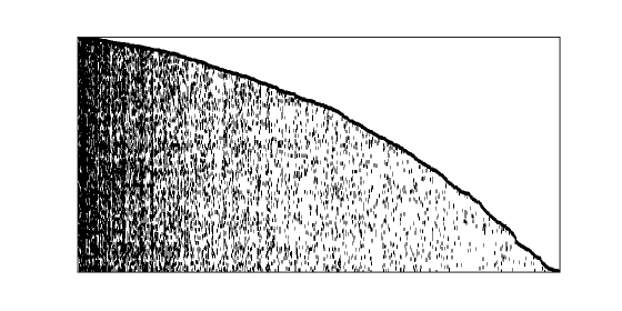
Figure 1: IEEE Automatic Driving dataset. Observed actions-features matrix with dimensions $T\times L_{T}=492\times 4553$. Black dots represent $1$ while white dots represent $0$.

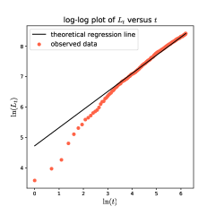
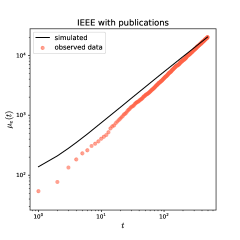
Figure 2: IEEE Automatic Driving dataset. Left: Plot of $\ln(L_{t})$ as a function of $\ln(t)$, with the power-law trend. The red dots refer to the real data and the black line gives the theoretical regression line with slope $\widehat{\beta}$. Right: Asymptotic behavior of the number of edges in the actions-features network. Red dots refer to $e(t)$ of the real data, while the black line shows $\mu_{e}(t)$ obtained by the model with $G_{t,i}^{pub}$ (averaging over $R=100$ simulations).

For this application, we use weights of the type 3), Sec. 3.2. Indeed, at each time-step $t$, we associate to each author $i$ a “fitness” variable $G_{t,i}$ that quantifies the influence of author $i$ in the considered research field, and we define the weights as

$$\begin{split}W_{t,j,k}&=W_{t,j}=e^{-1/M_{t,j}}\;\hbox{ with }\;M_{t,j}=\max\{G_{t,i}:\,i\in\mathcal{I}(j)\}\;\hbox{where}\;\\ \mathcal{I}(j)&=\hbox{set of the agents performing action $j$}\,.\end{split}$$ (5)

Therefore the inclusion probability in equation (2) reads as

$$P_{t}(k)=\frac{\delta}{2}+(1-\delta)\frac{\sum_{j=1}^{t-1}F_{j,k}\,e^{-1/M_{t,j}}}{t}.$$ (6)

The term $M_{t,j}$ is the maximum among the fitness variables $G_{t,i}$ at time-step $t$ of all the authors $i\in{\mathcal{I}}(j)$, i.e. the authors who published the paper appeared at time-step $j$. A high value of $G_{t,i}$ should identify a person who is relevant in the considered research field so that it is likely that other scholars use the same features of her/his actions, that essentially are the keywords related to her/his research. As a consequence, in the preferential attachment term, we give to each old feature $k$ a weight that is increasing with respect to the fitness variables of the authors who included $k$ in their papers. We analyse two different fitness variables:

$$G_{t,i}^{pub}=\hbox{(total number of author $i$'s publications until time-step $t-1$)}+1$$ (7)

and

$$G_{t,i}^{col}=\hbox{(total number of author $i$'s collaborators until time-step $t-1$)}+1.$$ (8)

(Note that we count publications or collaborators until time-step $t-1$, that is until a time-step before the record time of paper $t$ and $1$ is added in order to avoid division by zero in the previous formula (5).)

$p$	$\widehat{p}$	$\overline{p}$	$MSE(p)$
$\alpha$	$68.534$	$68.699$	$14.699$
$\beta$	$0.5962$	$0.5962$	$0.0001$
$\delta$ with $G_{t,i}^{pub}$	$\approx 2.22\cdot 10^{-16}$	$\approx 4.36\cdot 10^{-5}$	$\approx 5.90\cdot 10^{-9}$
$\delta$ with $G_{t,i}^{col}$	$\approx 2.26\cdot 10^{-16}$	$\approx 5.01\cdot 10^{-5}$	$\approx 6.82\cdot 10^{-9}$

Table 1: IEEE Automatic Driving dataset. Estimation of the model parameters. The average values $\overline{p}$ and the parameters’ $MSE$ are computed over $R=100$ realizations of the model. See Subsection A.3 for further details.

Matrix	$L_{T}$	$\sigma_{L_{T}}$	$\overline{O}_{T}$	$\sigma_{O_{T}}$	$\overline{N}_{T}$	$\sigma_{N_{T}}$
real	$4553$		$31.54$		$9.25$
Weights with $G_{t,i}^{pub}$	$4558$	$68.19$	$\mathbf{32.13}$	$1.29$	$9.26$	$0.14$
Weights with $G_{t,i}^{col}$	$4548$	$63.00$	$54.20$	$2.88$	$9.25$	$0.13$
Weights = 1	$4551$	$71.50$	$134.73$	$3.48$	$9.25$	$0.15$

Table 2: IEEE Automatic Driving dataset. Comparison between real and simulated actions-features matrices by means of the indicators (24). For the simulations, all the considered quantities have been averaged over $R=100$ realizations of the model. We also include an estimate of the variations around the averaged values, through the computation of the sample standard deviations. See Subsection A.3 for further details.

Weights with $G_{t,i}^{pub}$	$\overline{m}_{1}$	$\overline{m}_{2}$
$k^{*}=4553$ (all observed features)	$\mathbf{0.97}$	$0.047$
$k^{*}=100$	$\mathbf{0.88}$
$k^{*}=200$	$\mathbf{0.90}$
$k^{*}=300$	$\mathbf{0.91}$

Weights with $G_{t,i}^{col}$	$\overline{m}_{1}$	$\overline{m}_{2}$
$k^{*}=4553$ (all observed features)	$0.96$	$0.049$
$k^{*}=100$	$0.83$
$k^{*}=200$	$0.86$
$k^{*}=300$	$0.88$

Weights = 1	$\overline{m}_{1}$	$\overline{m}_{2}$
$k^{*}=4553$ (all observed features)	$0.93$	$0.049$
$k^{*}=100$	$0.55$
$k^{*}=200$	$0.64$
$k^{*}=300$	$0.70$

Table 3: IEEE Automatic Driving dataset. Comparison between real and simulated actions-features matrices by means of the indicators (25). The first row of each table evaluates the indicators on the whole matrix ($k^{*}=4553$), while the other rows show the results computing the indicator $\overline{m}_{1}$ only on the first $k^{*}$ ($=100,\,200,\,300$) features. See Subsection A.3 for further details.

Weights with $G_{t,i}^{pub}$	$\overline{m}_{1}^{*}$	$\overline{m}_{2}^{*}$
$T^{*}=369$ and $k^{*}=4553$	$0.99$	$0.017$
$T^{*}=246$ and $k^{*}=4553$	$0.98$	$0.060$
$T^{*}=123$ and $k^{*}=4553$	$0.98$	$0.113$
$T^{*}=369$ and $k^{*}=200$	$0.93$
$T^{*}=246$ and $k^{*}=200$	$0.93$
$T^{*}=123$ and $k^{*}=200$	$0.93$

Table 4: IEEE Automatic Driving dataset. Predictions on the actions-features matrix. The indicators (26) are computed for different levels of information used as “training set”: more precisely, the different $T^{*}$ correspond to $75\%$, $50\%$ and $25\%$ of the set of the actions, respectively. Moreover, the indicator $\overline{m}_{1}^{*}$ is computed on the whole matrix ($k^{*}=4553$) and also taking into account only the first $k^{*}=200$ features. See Subsection A.3 for further details.

For both the definitions of fitness, we perform the analysis following the methodology explained in Subsection A.3 (for the simulated matrices, all the considered quantities have been averaged over $R=100$ realizations of the model). We first estimate the model’s parameters, obtaining the results in Table 1. We can see that the weighted preferential attachment term (4) plays a predominant role, due to the estimated value obtained for the parameter $\delta$ that is approximately zero. Figure 2 provides in the left panel a log-log plot of the cumulative count of new features (key-words) as a function of time (see the red dots), that clearly shows a power-law behavior. This agrees with the theoretical property of the model stated in the Appendix, Subsec. A.1.1, according to which the power-law exponent has to be equal to the parameter $\beta$. This fact is checked in the plot by the black line, whose slope is the estimated value of the parameter $\beta$. The goodness of fit of our model to the dataset has been evaluated through the computation of the quantities (24) and (25). These results are shown in Table 2 and Table 3. Table 2 shows that our model reproduces the total number $L_{T}$ of features observed at the end of the observation period $T$, as well as the average number of new features $\overline{N}_{T}$ in all the three considered cases. The average number of old features (i.e. the quantity $\overline{O}_{T}$) is well reproduced only in the case with $G_{t,i}^{pub}$ (that is the case with the fitness based on the number of publications). Table 3 also indicates that the model with $G_{t,i}^{pub}$, or with $G_{t,i}^{col}$, shows a better performance than the one with all the weights equal to one. More precisely, the values obtained for the indicator $\overline{m}_{2}$ are almost the same for all the three cases (the average error on the total number of arrived features is around $5\%$); while the most significant differences are in the values of the indicator $\overline{m}_{1}$. Indeed, for the model with the fitness $G_{t,i}^{pub}$, the computed value of $\overline{m}_{1}$ ranges from $88\%$ to $97\%$, pointing out that a high percentage of the entries in the actions-features matrix have been correctly inferred by the model. The same value for the model with the fitness $G_{t,i}^{col}$ ranges from $83\%$ to $96\%$, and, for the model with all the weights equal to $1$, it ranges from $55\%$ to $93\%$. The differences with respect to the case with all the weights equal to $1$ are more evident when we select the first $k^{*}$ features: indeed, with $G_{t,i}^{pub}$ we succeed to infer the value of at least $88\%$ of the entries; while with all the weights equal to $1$ the percentage remains under $70\%$. This means that the major difference in the performance of the different considered weights is in the first features, that are those for which the preferential attachment term is more relevant. At this point, we choose the model that takes into account the authors’ number of publications as the best performing one for the considered dataset and in the following we focus on it. In Table 4 we evaluate the predictive power of the model: we estimate the parameters of the model only on a subset of the observed actions, respectively the $75\%$, $50\%$ and $25\%$ of the total observations; we then predict the features for the “future” actions $\{T^{*}+1,\dots,T\}$ and compare the predicted and observed results by means of the indicators in (26) over the whole set of features and only on a portion of it. The indicator $\overline{m}_{1}^{*}$ ranges from $93\%$ to $99\%$. Finally, in the right panel of Figure 2, we provide the asymptotic behavior of the number of edges in the actions-features network: more precisely, the red dots represent the total number $e(t)$ of edges observed in the real actions-features matrix at each time-step; while the continuous black line shows the mean number $\mu_{e}(t)$ of edges obtained averaging over $R=100$ simulations of the model with the chosen weights.

It is worth to note that the difference in the performance between the two definitions of fitness variables has a straightforward interpretation: in the considered case, i.e. for the publications in the area of Automatic Driving in the considered period, the relevance of an author (with respect to the probability of transmitting her/his features) is better measured by considering the number of her/his publications rather than the number of her/his co-authors. As we will see later on, we get a different result for our second application.

4.3 ArXiv dataset for Theoretical High Energy Physics

Our second application has been performed with the arXiv dataset of publications in the scientific area of Theoretical High Energy Physics (Hep-Th), recorded in the period $2000-2003$, freely available from [28]. The dataset collects a sample of text files reporting the full frontispiece of each paper, so we have information on: arXiv id number, date of submission, name and email of the author who made the submission, title, authors’ names and the entire text of the abstract. From the original format we isolate the submission date and the identity number of the paper, in order to sort all papers (actions) chronologically. Then, with the final purpose of constructing the features matrix, we consider all key-words included either in the main title or in the abstract as the features of the papers and we sort them according to their time of appearence. (The complete data preparation phase is described in the Appendix, Subsection A.3). We constructed the features matrix $F$, whose elements are equal to $F_{t,k}=1$ if paper $t$ includes word $k$ either in the title or in the abstract and $F_{t,k}=0$ otherwise. The result is shown in Figure 3, where the observed actions-features matrix collects $T=10603$ papers (actions) registered between $2000$ and $2003$ and $L_{T}=22304$ key-words appeared in the title or in the abstract (features), while the total number of involved authors (agents) is $n=5633$.

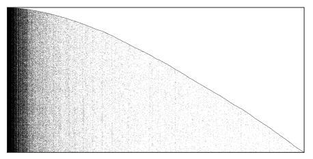
Figure 3: arXiv High Energy Physics dataset. Observed actions-features matrix with dimensions $T\times L_{T}=10603\times 22304$. Black dots represent $1$ while white dots represent $0$.

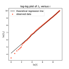
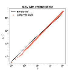
Figure 4: arXiv High Energy Physics dataset. Left: Plot of $\ln(L_{t})$ as a function of $\ln(t)$, with the power-law trend. The red dots refer to the real data and the black line gives the theoretical regression line with slope $\widehat{\beta}$. Right: Asymptotic behavior of the number of edges in the actions-features network. Red dots refer to $e(t)$ of the real data, while the black line shows $\mu_{e}(t)$ obtained by the model with $G_{t,i}^{col}$ (averaging over $R=100$ simulations).

$p$	$\widehat{p}$	$\overline{p}$	$MSE(p)$
$\alpha$	$40.812$	$40.940$	$2.4980$
$\beta$	$0.6305$	$0.6303$	$2.35\cdot 10^{-5}$
$\delta$ with $G_{t,i}^{pub}$	$\approx 2.22\cdot 10^{-16}$	$\approx 1.41\cdot 10^{-6}$	$\approx 5.55\cdot 10^{-12}$
$\delta$ with $G_{t,i}^{col}$	$\approx 2.22\cdot 10^{-16}$	$\approx 1.06\cdot 10^{-6}$	$\approx 3.44\cdot 10^{-12}$

Table 5: arXiv High Energy Physics dataset. Estimation of the model parameters. The average values $\overline{p}$ and the parameters’ $MSE$ are computed over $R=100$ realizations of the model. See Subsection A.3 for further details.

Matrix	$L_{T}$	$\sigma_{L_{T}}$	$\overline{O}_{T}$	$\sigma_{O_{T}}$	$\overline{N}_{T}$	$\sigma_{N_{T}}$
real	$22304$		$28.42$		$2.10$
Weights with $G_{t,i}^{pub}$	$22305$	$145.83$	$15.37$	$0.41$	$2.10$	$0.02$
Weights with $G_{t,i}^{col}$	$22317$	$148.35$	$18.79$	$0.70$	$2.10$	$0.02$
Weights = 1	$22313$	$147.35$	$97.16$	$5.16$	$2.10$	$0.02$

Table 6: arXiv High Energy Physics dataset. Comparison between real and simulated actions-features matrices by means of the indicators (24). For the simulations, all the considered quantities have been averaged over $R=100$ realizations of the model. We also include an estimate of the variations around the averaged values, through the computation of the sample standard deviations. See Subsection A.3 for further details.

Weights with $G_{t,i}^{pub}$	$\overline{m}_{1}$	$\overline{m}_{2}$
$k^{*}=22304$ (all observed features)	$0.995$	$0.022$
$k^{*}=5576$	$0.992$
$k^{*}=11152$	$0.994$
$k^{*}=16728$	$0.995$

Weights with $G_{t,i}^{col}$	$\overline{m}_{1}$	$\overline{m}_{2}$
$k^{*}=22304$ (all observed features)	$0.995$	$0.021$
$k^{*}=5576$	$0.991$
$k^{*}=11152$	$0.994$
$k^{*}=16728$	$0.994$

Weights = 1	$\overline{m}_{1}$	$\overline{m}_{2}$
$k^{*}=22304$ (all observed features)	$0.987$	$0.021$
$k^{*}=5576$	$0.976$
$k^{*}=11152$	$0.985$
$k^{*}=16728$	$0.986$

Table 7: arXiv High Energy Physics dataset. Comparison between real and simulated actions-features matrices by means of the indicators (25). The first row of each table evaluates the indicators on the whole matrix ($k^{*}=22304$), while the other rows show the results computing the indicator $\overline{m}_{1}$ only on the first $k^{*}$ ($=5576,\,11152,\,16728$) features. See Subsection A.3 for further details.

The weights for this application are defined as in the previous one, described in equation (5). We consider again the two different definitions for the “fitness” term $G_{t,i}$ (see (7) and (8)). The performed analysis follows the outline explained in Subsection A.3 (for the simulated matrices, all the considered quantities have been averaged over $R=100$ realizations of the model). We first estimate the model’s parameters, obtaining the results in Table 5. We see that the weighted preferential attachment term (4) gives most of the contribution due to the estimated value obtained for the parameter $\delta$ that is essentially zero. Figure 4 provides in the left panel a log-log plot of the cumulative count of new features (key-words) as a function of time (see the red dots), that clearly shows a power-law behavior. This agrees with the theoretical property of the model stated in the Appendix, Subsec. A.1.1, according to which the power-law exponent has to be equal to the parameter $\beta$. This fact is checked in the plot by the black line, which slope is the estimated value of the parameter $\beta$. The goodness of fit of our model to the dataset has been evaluated through the computation of the quantities (24) and (25). These results are shown in Table 6 and Table 7. Table 6 shows that our model is able to reproduce the total number $L_{T}$ of features observed at the end of the observation period $T$ and the average number of new features $\overline{N}_{T}$. Instead, the average number of old features (i.e. the quantity $\overline{O}_{T}$) is under-estimated by the model with the weights based on $G_{t,i}^{pub}$ and $G_{t,i}^{col}$, while it is widely over-estimated in the case with all the weights equal to $1$. The discrepancy in the values is smaller for the case with $G_{t,i}^{col}$ (that is the case with the fitness based on the number of collaborators). Table 7 shows that the performance of the model in reproducing the data are comparable, with both the considered definitions of fitness and they are also good for the case with all weights equal to one. At this point, we choose the model that takes into account the authors’ number of collaborations and the last analysis focuses on it. In Table 8 we evaluate the predictive power of the model: we estimate the parameters of the model only on a subset of the observed actions, respectively the $75\%$, $50\%$ and $25\%$ of the total observations; we then predict the features for the “future” actions $\{T^{*}+1,\dots,T\}$ and compare the predicted and observed results by means of the indicators in (26) over the whole set of features and only on a portion of it. In particular, we obtain that the indicator $\overline{m}_{1}^{*}$ is almost always equal to $99\%$. Finally, in the right panel of Figure 4, we provide the asymptotic behavior of the number of edges in the actions-features network: more precisely, the red dots represent the total number $e(t)$ of edges observed in the real actions-features matrix at each time-step; while the continuous black line shows the mean number $\mu_{e}(t)$ of edges obtained averaging over $R=100$ simulations of the model with the chosen weights.

Weights with $G_{t,i}^{col}$	$\overline{m}_{1}^{*}$	$\overline{m}_{2}^{*}$
$T^{*}=7952$ and $k^{*}=22304$	$0.997$	$0.006$
$T^{*}=5302$ and $k^{*}=22304$	$0.997$	$0.026$
$T^{*}=2651$ and $k^{*}=22304$	$0.996$	$0.035$
$T^{*}=7952$ and $k^{*}=11152$	$0.996$
$T^{*}=5302$ and $k^{*}=11152$	$0.996$
$T^{*}=2651$ and $k^{*}=11152$	$0.996$

Table 8: arXiv High Energy Physics dataset. Predictions on the actions-features matrix. The indicators (26) are computed for different levels of information used as “training set”: more precisely, the different $T^{*}$ correspond to $75\%$, $50\%$ and $25\%$ of the set of the actions, respectively. Moreover, the indicator $\overline{m}_{1}^{*}$ is computed on the whole matrix ($k^{*}=22304$) and also taking into account only the first $k^{*}=11152$ features. See Subsection A.3 for further details.

Contrarily to the previous case, in this application we observe a comparable performance of the model with both the considered definitions of fitness. This means that, for the publications in High Energy Physics in the considered period, both the number of co-authors and the number of publications of an author can be considered as reasonable measures in order to evaluate her/his relevance in the research field.

4.4 Instagram dataset

The dataset used for this application has been kindly provided by Prof. Emilio Ferrara and a more detailed description can be found in [29]. The dataset has been crawled through the Instagram API between January 20 and February 17, 2014 and collects public media (with their author, timestamp and set of hashtags) as well as users information (with their list of followers and followees) of a set of $2100$ anonymized partecipants to $72$ popular photographic contests that took place between October $2010$ and February $2014$. The overall media dataset records more than one million posts but, with the purpose of maximizing the density of our actions-features matrix, we considered only those posts posted during the weekends in the crawling period (Jan 20$-$Feb 17, 2014) in which at least $5$ hashtags are used. This procedure yields a sample of $T=2151$ posts (actions) and $L_{T}=5890$ hashtags (features). The available posts were ordered chronologically according to the associate timestamp of publication and the hashtags (features) were sorted in terms of their first appearence in a post. After this first phase of data arrangement, we constructed the actions-features matrix $F$, with $F_{t,k}=1$ if post $t$ contains hashtag $k$ and $F_{t,k}=0$ otherwise. The resulting matrix is shown in Figure 5, with non-zero values indicated by black points.

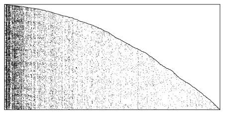
Figure 5: Instagram dataset. Observed actions-features matrix, with dimesions $T\times L_{T}=2151\times 5890$. Black dots represent $1$ while white dots represent $0$.

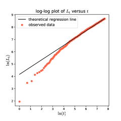
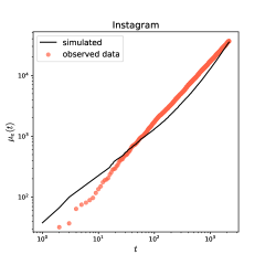
Figure 6: Instagram dataset. Left: Plot of $\ln(L_{t})$ as a function of $\ln(t)$, with the power-law trend. The red dots refer to the real data and the black line gives the theoretical regression line with slope $\widehat{\beta}$. Right: Asymptotic behavior of the number of edges in the actions-features network. Red dots refer to $e(t)$ of the real data, while the black line shows $\mu_{e}(t)$ obtained by the model (averaging over $R=100$ simulations).

For this application, we chose weights of type 5), Subsection 3.2, that depend on an indicator related to the underlying Instagram network. Precisely, we associate to each agent $i$ the variable $G_{i}$ defined as the number of agents $i$’s followers, among those who were active during the crawling period and we set

$$W_{t,j,k}=W_{t}=e^{-G_{i(t)}},$$ (9)

where $i(t)$ denotes the agent performing action $t$. Therefore the inclusion probability for hashtag $k$ becomes

$$P_{t}(k)=\frac{\delta}{2}+(1-\delta)\ \frac{\sum_{j=1}^{t-1}F_{j,k}}{t}\;e^{-G_{i(t)}}\,,$$ (10)

where the average popularity of hashtag $k$ is exponentially discounted by the factor $G_{i(t)}$. The decision to introduce such kind of weights was driven by the following consideration. A user with a very high number of followers identifies a person who is very popular on the social networks, an “influencer” in the extreme case. As a consequence, it may be reasonable to think that she/he is less affected by other people’s posts and, consequently, less prone to use “old” hashtags. For this user, the average popularity of $k$ in the inclusion probability $P_{t}(k)$ should be less relevant. On the contrary, a user with a low number of followers may be more incline to follow the current trends and the others’ preferences and choices. It is worthwhile to point out that in the definition of the weights, we considered the number of followers of an user as fixed to the value we observed at the end of the period of observation (the crawling period). In general, it may change in time, depending on the changes in her/his network of “virtual friendships”. However, we assume it to be constant because of the short time span considered.

$p$	$\widehat{p}$	$\overline{p}$	$MSE(p)$
$\alpha$	37.895	37.843	4.516
$\beta$	0.5897	0.5900	$7.89\cdot 10^{-5}$
$\delta$ with weights (9)	0.0063	0.0062	$2.70\cdot 10^{-8}$

Table 9: Instagram dataset: Estimation of the model parameters. The average values $\overline{p}$ and the parameters’ $MSE$ are computed over $R=100$ realizations of the model. See Subsection A.3 for further details.

Matrix ($T=2151$)	$L_{T}$	$\sigma_{L_{T}}$	$\overline{O}_{T}$	$\sigma_{O_{T}}$	$\overline{N}_{T}$	$\sigma_{N_{T}}$
real	$5890$		$14.23$		$2.74$
Weights (9)	$5885$	$42.39$	$\mathbf{13.56}$	$0.24$	$2.74$	$0.02$
Weights = 1	$5899$	$73.00$	$80.03$	$5.20$	$2.74$	$0.04$

Table 10: Instagram dataset. Comparison between real and simulated actions-features matrices by means of the indicators (24). For the simulations, all the considered quantities have been averaged over $R=100$ realizations of the model. We also include an estimate of the variations around the averaged values, through the computation of the sample standard deviations. See Subsection A.3 for further details.

Weights (9)	$\overline{m}_{1}$	$\overline{m}_{2}$
$k^{*}=5890$ (all observed features)	0.99	0.037
$k^{*}=100$	0.97
$k^{*}=250$	0.98
$k^{*}=500$	0.98

Weights = 1	$\overline{m}_{1}$	$\overline{m}_{2}$
$k^{*}=5890$ (all observed features)	0.97	0.037
$k^{*}=100$	0.63
$k^{*}=250$	0.77
$k^{*}=500$	0.86

Table 11: Instagram dataset. Comparison between real and simulated actions-features matrices by means of the indicators (25). The first row of each table evaluates the indicators on the whole matrix ($k^{*}=5890$), while the other rows show the results computing the indicator $\overline{m}_{1}$ only on the first $k^{*}$ ($=100,\,250,\,500$) features. See Subsection A.3 for further details.

Weights (9)	$\overline{m}_{1}^{*}$	$\overline{m}_{2}^{*}$
$T^{*}=1613$ and $k^{*}=5890$	0.99	0.006
$T^{*}=1076$ and $k^{*}=5890$	0.99	0.031
$T^{*}=538$   and $k^{*}=5890$	0.99	0.099
$T^{*}=1613$ and $k^{*}=250$	0.98
$T^{*}=1076$ and $k^{*}=250$	0.98
$T^{*}=538$   and $k^{*}=250$	0.97

Table 12: Instagram dataset. Predictions on the actions-features matrix. The indicators (26) are computed for different levels of information used as “training set”: more precisely, the different $T^{*}$ correspond to 75%, 50% and 25% of the set of the actions, respectively. Moreover, the indicator $\overline{m}_{1}^{*}$ is computed on the whole matrix ($k^{*}=5890$) and also taking into account only the first $k^{*}=250$ features. See Subsection A.3 for further details.

The performed analysis follows the outline explained in Subsection A.3 (for the simulated matrices, all the considered quantities have been averaged over $R=100$ realizations of the model). We first estimate the model’s parameters, obtaining the results in Table 9. The weighted preferential attachment term (4) plays an important role, but slightly lower than in the previous cases, since the inclusion probability is obtained with $\delta=0.6\%$. Figure 6 provides in the left panel a log-log plot of the cumulative count of new features (hashtags) as a function of time (see the red dots), that clearly shows a power-law behavior. This agrees with the theoretical property of the model stated in the Appendix, Subsec. A.1.1, according to which the power-law exponent has to be equal to the parameter $\beta$. This fact is checked in the plot by the black line, whose slope is the estimated value of the parameter $\beta$. The goodness of fit of our model to the dataset has been evaluated through the computation of the quantities (24) and (25). These results are shown in Table 10 and Table 11. Table 10 shows that our model is perfectly able to reproduce the total number $L_{T}$ of features observed at the end of the observation period $T$, as well as the average number of new features $\overline{N}_{T}$ in both the considered cases. The average number of old features (i.e. the quantity $\overline{O}_{T}$) shows a good agreement with the observed quantity in the case of the model with the chosen weights, contrarily to the model with all the weights equal to one for which we obtain a much higher value. Table 11 also indicates that the model with the chosen weights shows a better performance than the one with all the weights equal to one. More precisely, the values obtained for the indicator $\overline{m}_{2}$ are almost the same for both cases (the average error on the total number of arrived features is around $4\%$); while the most significant differences are in the values of the indicator $\overline{m}_{1}$. Indeed, for the model with the chosen weights, the computed values of $\overline{m}_{1}$ ranges from $97\%$ to $99\%$, pointing out that a high percentage of the entries in the actions-features matrix have been correctly inferred by the model. The differences are more evident when we select the first $k^{*}$ features: indeed, with the chosen weights we succeed to infer the values of at least $97\%$ of the entries; while with all the weights equal to $1$ the percentage remains under $86\%$. This means that the major difference in the performance of the different considered weights is in the first features, that are those for which the preferential attachment term is more relevant. In Table 12 we evaluate the predictive power of the model with the chosen weights: we estimate the parameters of the model only on a subset of the observed actions, respectively the $75\%$, $50\%$ and $25\%$ of the total observations; we then predict the features for the “future” actions $\{T^{*}+1,\dots,T\}$ and compare the predicted and observed results by means of the indicators in (26) over the whole set of features and only on a portion of it. The indicator $\overline{m}_{1}^{*}$ ranges from $97\%$ to $99\%$. Finally, in the right panel of Figure 6, we provide the asymptotic behavior of the number of edges in the actions-features network: more precisely, the red dots represent the total number $e(t)$ of edges observed in the real actions-features matrix at each time-step; while the continuous black line shows the mean number $\mu_{e}(t)$ of edges obtained averaging over $R=100$ simulations of the model with the chosen weights.

4.5 Summary of the results

We here summarize the major findings of the three considered applications.

In all the three cases we selected the weights depending on a fitness variable. In the first two applications (IEEE and arXiv), the fitness variable measures the “ability” of the agents (authors) to transmit the features (keywords) of their actions (publications). In the third application (Instragram) the fitness variable quantifies the “inclination” of the agents (users) to follow the features (hashtags) of the previous actions (posts). From the performed analyses of the actions-features bipartite networks, we get the following main common issues for the three applications:

• The preferential attachment rule plays a relevant role in the formation of the actions-features network, because of the small estimated values obtained for the parameter $\delta$. In particular, in the first two applications, the estimated value of $\delta$ is very close to zero.

• The considered indicators (24), (25) and (26), and the plots regarding the behaviors along time of the total number of observed features $L_{t}$ and the total number of edges $e(t)$ show a good fit between the model with the chosen weights and the real datasets. In particular, the power-law behavior of $L_{t}$ perfectly matches the theoretical one with the estimated parameter $\beta$ as the power-law exponent, and a high percentage of the entries of the actions-features matrix is successfully inferred with the model. Moreover, a good performance is also obtained when making a prediction analysis, i.e. testing the percentage of the entries that are successfully recovered by the model providing it with different levels of information.

• With respect to the “flat weights”, i.e. all weights equal to $1$, the chosen weights guarantee a better agreement with the real actions-features matrices. Among the indicators in (24), the one that mostly put in evidence this fact is $\overline{O}_{T}$. Moreover, the difference in the performance of the model with different weights is also particularly evident when we consider a subset of the overall set of observed features for the computation of the indicators $\overline{m}_{1}$ in (25) and $\overline{m}_{1}^{*}$ in (26). Indeed, the first features are those for which the preferential attachment term is more relevant.

5 Discussion and conclusions

In this work we have presented our contribution to the stream of literature regarding stochastic models for bipartite networks formation. With respect to the previous publications, our paper introduces some novelties. First of all, given a system of agents, we are not interested in modeling the process of link formation between the agents themselves, we instead define a model that describes the activity of the agents, studying the behavior in time of agents’ actions and the features shown by these actions. This issue allows to amplify the range of possible applications, since we only assume to know the chronological order in which we observe the agents’ actions, and not the order in which the agents arrive. Second, we extend the concept of “preferential attachment with weights” [10, 11] to this framework. The weights can have different forms and meanings according to the specific setting considered and play an important role since the probability that a future action shows a certain feature depends, not only on its “popularity” (i.e. the number of previous actions showing the feature) as stated by the preferential attachment rule, but also on some characteristics of the agents and/or the features themselves. For instance, the weights may give information regarding the “ability” of an agent to transmit the features of her/his actions to the future actions, or the “inclination” of an agent to adopt the features shown in the past.
Summarizing, we first provide a full description of the model dynamics and interpretation of the included parameters and variables, also showing some theoretical results regarding the asymptotic properties of some important quantities. Moreover, we illustrate the necessary tools in order to estimate the parameters of the model and we consider three different applications. For each of them, we evaluate the goodness of fit of the model to the data by checking the theoretical asymptotic properties of the model in the real data, by comparing several indicators computed both on the real and simulated matrices, as well as testing the ability of the model as a predictive instrument in order to forecast which features will be shown by future actions. All our analyses point out a very good fit of our model and a very good performance of the adopted tools in all the three considered cases.
Our model and the related analysis have been able to detect some interesting aspects that characterize the different examined contexts. In the first two applications (IEEE and arXiv) we examined the publications in the scientific areas of Automatic Driving and of High Energy Physics (briefly Hep-Th) and we took into account two kinds of fitness variables for the authors: one based on the number of publications and the other based on the number of collaborators. Our study reveals that, for Hep-Th, both the number of publications of an author and the number of her/his collaborators are able to provide a good agreement with real data, while, for Automatic Driving, we found a better performance of the model with the weights based on the number of publications. Probably this difference is due to the fact that, while the Physics of High Energies is quite an old subject in which different branches developed, Automatic Driving is a much younger, and so limited, research area. (Indeed, the observed values of $T$ and $L_{T}$, that is the number of publications and the number of keywords in the considered period, for the Automatic Driving are much smaller than the ones observed for Hep-Th. The indicator $\overline{N}_{T}$ also suggests that Automatic Driving is a much younger research field than Hep-Th, since the observed value for the former is much greater than the one for the latter.) The behavior of on-line social networks is completely different: we examine the dataset of Instagram, with posts considered as actions and hashtag as features. Indeed, we saw that the less followers a user has the higher the number of “old” hashtag used. This could be related to the fact that less popular users tend to re-use many “old” hashtags in order to increase their visibility, while highly famous users do not feel the need of improving their popularity in this way and focus on few “old” hashtags. Indeed, this behavior show a completely different role of the “on-line followership” relations respect to coauthorships: while collaborations incentive the usage of a high number of existing features, the number of followers takes to a limited usage of existing hashtags.

Competing interests statement

The authors have no competing interests to declare.

Appendix A Appendix

In the appendix we collect all the technical results and details that, for the sake of simplicity, have not been included in the main body of the work. Specifically, in Subsection A.1 we describe the asymptotic behavior of the total number of features along time and we show some analytical findings regarding the asymptotic behavior of the mean number of edges in the actions-features bipartite network; in Subsection A.2 we provide some statistical tools in order to estimate the parameters of the model; finally, in the last Subsection A.3, we illustrate the indicators used in order to analyze the three considered real datasets (arXiv, IEEE, Instagram).

A.1 Some asymptotic results for the model

We here illustrate some asymptotic properties of the model.

A.1.1 Asymptotic behavior of the total number of features

The random variable $L_{t}=\sum_{j=1}^{t}N_{j}$, that represents the total number of features present in the system at time-step $t$, has the following asymptotic behaviors as $t\to+\infty$:

• for $\beta=0$, we have a logarithmic behavior of $L_{t}$, that is $L_{t}/\ln(t)\to\alpha$ almost surely;

• for $\beta\in(0,1]$, we obtain a power-law behavior, i.e. $L_{t}/t^{\beta}\to\alpha/\beta$ almost surely.

The proof of these two statements is exactly the same as in [24], since the weights do not affect $L_{t}$.

A.1.2 Asymptotic behavior of the mean number of edges in the actions-features network

We here analyze the asymptotic behavior, as $t\to+\infty$, of $\mu_{e}(t)=E[e(t)]$, where $e(t)$ is the total number of edges in the actions-features network at time-step $t$, that is the total number of ones in the matrix $F$ until time-step $t$. A first remark is that we have

$$e(t)=\sum_{u=1}^{t}\sum_{k:\,T_{k}=u}d_{k}(t),$$ (11)

where we denote by $T_{k}$ the arrival time-step of feature $k$ and

$$d_{k}(t)=\sum_{j=1}^{t}F_{j,k}=1+\sum_{j=T_{k}+1}^{t}F_{j,k}$$ (12)

is the degree of feature $k$ at time-step $t$. Hence, we can write

$$E[e(t)|T_{k}\;\forall k\,\mbox{with }T_{k}\leq t]=\sum_{u=1}^{t}\mbox{card}(k:\,T_{k}=u)E[d_{k}(t)|T_{k}=u]=\sum_{u=1}^{t}N_{u}E[d_{k}(t)|T_{k}=u],$$ (13)

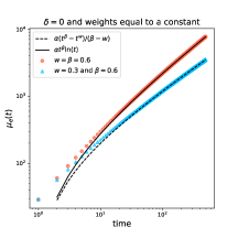
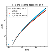
Figure 7: Evolution of $\mu_{e}(t)$, i.e. the mean number of edges along time. From top-left to bottom-right we have the cases: $\delta=1$ and weights equal to $1$; $\delta=0$ and weights equal to a constant $w$ (the blue triangles represent the case with $w\neq\beta$, while the red dots show the case $w=\beta$); $\delta=0$ and weights depending only on $t$ with uniform distribution on $[0,1]$ (the blue triangles show the case with the mean value $\mu_{W}\neq\beta$, while the red dots describe the case with $\mu_{W}=\beta$); $\delta=0$ and weights depending only on $k$, considering the two different distributions of the provided examples (uniform and truncated exponential distribution) for the weights: the continuous lines refer to the values of the integrals (18) and (19), respectively, while the dashed lines show the final approximations. All simulations have been performed with $\alpha=30$ and $\beta=0.6$ (unless otherwise specified in the legend).

where we recall that $N_{u}$ is Poi$(\lambda_{u})$-distributed with $\lambda_{u}=\alpha/u^{1-\beta}$. In the following subsections, we go further with the computations in the two “extreme” cases $\delta=1$ and $\delta=0$ since the behavior for a general $\delta$ is a mixture of the two behaviors in the extreme cases. A graphical representation of the evolution of $\mu_{e}(t)$ in the considered cases is provided in Figure 7 (the values are averaged over a sample of $R=100$ simulations).

The case $\delta=1$

In this case the inclusion probability of a feature $k$ at time-step $t$ simply is $P_{t}(k)=\dfrac{1}{2}$. Therefore, since (12), we have

$$E[d_{k}(t)|T_{k}=t_{k}]=1+\dfrac{t-t_{k}}{2}\sim t/2.$$

Hence, by (13) and the above approximation, we can approximate $\mu_{e}(t)$ by the quantity

$$\dfrac{t}{2}\sum_{u=1}^{t}\lambda_{u}=\dfrac{\alpha t}{2}\sum_{u=1}^{t}u^{\beta-1}\sim\dfrac{\alpha t^{1+\beta}}{2\beta}.$$ (14)

The case with $\delta=0$ and the weights equal to a constant

Let us assume $\delta=0$ and $W_{t,j,k}$ equal to a constant $w\in]0,1]$ for all $t,j,k$, so that the inclusion probability of a feature $k$ at time-step $t$ is

$$P_{t}(k)=\dfrac{d_{k}(t-1)}{t}w.$$

Let us set $\langle d_{k}(t)\rangle=E[d_{k}(t)|T_{k}=t_{k}]$ and observe that we have

$$\begin{split}\langle d_{k}(t)\rangle=&1+w\sum_{\tau=t_{k}+1}^{t}\dfrac{\langle d_{k}(\tau-1)\rangle}{\tau}\\ =&1+w\Bigg{[}\sum_{\tau=t_{k}+1}^{t-1}\dfrac{\langle d_{k}(\tau-1)\rangle}{\tau}+\dfrac{\langle d_{k}(t-1)\rangle}{t}\Bigg{]}\\ =&1+w\sum_{\tau=t_{k}+1}^{t-1}\dfrac{\langle d_{k}(\tau-1)\rangle}{\tau}+\dfrac{w}{t}\Bigg{[}1+w\sum_{\tau=t_{k}+1}^{t-1}\dfrac{\langle d_{k}(\tau-1)\rangle}{\tau}\Bigg{]}\\ =&\Big{(}1+\dfrac{w}{t}\Big{)}\Bigg{[}1+w\sum_{\tau=t_{k}+1}^{t-1}\dfrac{\langle d_{k}(\tau-1)\rangle}{\tau}\Bigg{]}\\ =&\cdots\\ =&\Big{(}1+\dfrac{w}{t}\Big{)}\Big{(}1+\dfrac{w}{t-1}\Big{)}\cdots\Big{(}1+\dfrac{w}{t_{k}+1}\Big{)}\\ =&\dfrac{t_{k}!}{t!}\cdot(t+w)\cdot(t-1+w)\cdots(t_{k}+1+w)\\ =&\dfrac{t_{k}!}{t!}\cdot\dfrac{(t+w)\cdot(t-1+w)\cdots(t_{k}+1+w)\cdot(t_{k}+w)\cdots(w+1)\cdot w}{(t_{k}+w)\cdots(w+1)\cdot w}.\end{split}$$

Using the properties of the $\Gamma$-function, we can write

$$\begin{split}\langle d_{k}(t)\rangle=&\dfrac{t_{k}!}{t!}\dfrac{\Gamma(t+w+1)!}{\Gamma(t_{k}+w+1)!}=\dfrac{\Gamma(t_{k}+1)}{\Gamma(t+1)}\dfrac{\Gamma(t+w+1)!}{\Gamma(t_{k}+w+1)!}\sim\Big{(}\dfrac{t}{t_{k}}\Big{)}^{w}.\end{split}$$ (15)

Therefore, by (13) and the above approximation, we can approximate $\mu_{e}(t)$ by the quantity

$$\sum_{u=1}^{t}\lambda_{u}\dfrac{t^{w}}{u^{w}}=\alpha t^{w}\sum_{u=1}^{t}u^{\beta-w-1}\sim\begin{cases}\alpha t^{\beta}\ln(t)\quad&\mbox{if }w=\beta,\\ \dfrac{\alpha}{\beta-w}(t^{\beta}-t^{w})\sim\dfrac{\alpha t^{\max\{w,\beta\}}}{|w-\beta|}\quad&\mbox{if }w\neq\beta.\end{cases}$$ (16)

Remark: It is worthwhile to note that in the case of weights of the form $W_{t,j,k}=W_{t}$ for all $t,j,k$, where the random variables $W_{t}$ take values in $[0,1]$, are identically distributed with mean value equal to $\mu_{W}$, and each of them is independent of all the past until time-step $t-1$, we get for $\mu_{e}(t)$ the same asymptotic behavior as above, but with $w=\mu_{W}$.

The case with $\delta=0$ and the weights depending only on $k$

Let us assume $\delta=0$ and $W_{t,j,k}=W_{k}$ for all $t,j,k$, where the random variables $W_{k}$ take values in $[0,1]$, are independent and identically distributed with probability density function $\rho$, and each of them independent of the arrival time-step $T_{k}$ of the feature. Moreover, we focus on the case $\beta<1$, that is more interesting then the case $\beta=1$. In this case the inclusion probability is

$$P_{t}(k)=\dfrac{d_{k}(t-1)}{t}W_{k}.$$

Using the same computations done above, we get

$$E[d_{k}(t)|T_{k}=t_{k},\,W_{k}]\sim\Big{(}\dfrac{t}{t_{k}}\Big{)}^{W_{k}}$$

and so we can approximate $E[d_{k}(t)|T_{k}=t_{k}]$ by $\int_{0}^{1}\left(\dfrac{t}{t_{k}}\right)^{w}\rho(w)\,dw$. Hence, using (13), we can approximate $\mu_{e}(t)$ by

$$\begin{split}&\sum_{u=1}^{t}\lambda_{u}\int_{0}^{1}\left(\dfrac{t}{u}\right)^{w}\rho(w)dw=\int_{0}^{1}t^{w}\sum_{u=1}^{t}\lambda_{u}u^{-w}\rho(w)dw=\\ &\alpha\int_{0}^{1}t^{w}\sum_{u=1}^{t}u^{-(w-\beta+1)}\rho(w)dw=\alpha t^{\beta}\int_{0}^{1}\dfrac{t^{w-\beta}-1}{w-\beta}\rho(w)dw.\end{split}$$ (17)

Therefore the asymptotic behavior of $\mu_{e}(t)$ depends on the asymptotic behavior of the above integral. In the sequel we analyze the case of the uniform distribution and the one of the “truncated” exponential distribution. To this purpose, we employ the Exponential integral

$$\text{Ei}(y)=-\int_{-y}^{+\infty}\dfrac{e^{-x}}{x}dx=\int_{-\infty}^{y}\dfrac{e^{v}}{v}dv,$$

which has the property $\lim_{y\rightarrow+\infty}\frac{e^{y}}{y\text{Ei}(y)}=1$.

Example 1 (Uniform distribution on $[0,1]$)
If $\rho(w)=1,\,\forall w\in[0,1]$ and equal to zero otherwise, we can compute the above integral and approximate $\mu_{e}(t)$ by

$$\alpha t^{\beta}\left\{\int_{-\beta\ln(t)}^{(1-\beta)\ln(t)}\dfrac{e^{v}}{v}dv-\int_{-\beta}^{1-\beta}\dfrac{1}{v}dv\right\}=\alpha t^{\beta}\Big{\{}\text{Ei}[(1-\beta)\ln(t)]-\text{Ei}[-\beta\ln(t)]+\ln\Big{(}\dfrac{\beta}{1-\beta}\Big{)}\Big{\}}$$ (18)

Using the asymptotic properties of the Exponential integral, we find that the above quantity behavies for $t\to+\infty$ as

$$\dfrac{\alpha t}{(1-\beta)\ln(t)}.$$

Example 2 (Exponential distribution on $[0,1]$)
If $\rho(w)=e^{1-w}/(e-1)$ for $w\in[0,1]$ and equal to zero otherwise, the computation of the above integral leads to the approximation for $\mu_{e}(t)$ given by

$$\begin{split}&\dfrac{\alpha e^{1-\beta}}{(e-1)}t^{\beta}\left\{-\int_{-\beta}^{1-\beta}\dfrac{e^{-x}}{x}dx+\int_{-\beta(\ln(t)-1)}^{(1-\beta)(\ln(t)-1)}\dfrac{e^{v}}{v}dv\right\}\\ &=\dfrac{\alpha e^{1-\beta}}{(e-1)}t^{\beta}\Big{\{}\text{Ei}[\beta]-\text{Ei}[-(1-\beta)]+\text{Ei}[(1-\beta)(\ln(t)-1)]-\text{Ei}[-\beta(\ln(t)-1)]\Big{\}}.\end{split}$$ (19)

Using the asymptotic properties of the Exponential integral, we find that the asymptotic behavior for $t\to+\infty$ of the above quantity is given by

$$\dfrac{\alpha t}{(e-1)(1-\beta)\ln(t)}.$$

A.2 Estimation of the model parameters

We here provide some statistical tools in order to estimate the parameters of the model introduced in Section 2.

The parameters $\alpha$ and $\beta$

The parameters $\alpha$ and $\beta$ can be estimated using a maximum likelihood method, that is maximizing the probability to observe $\{N_{1}=n_{1},N_{2}=n_{2},\dots,N_{T}=n_{T}\}$. Since all the random variables $N_{t}$ are assumed independent Poisson distributed, we have

$$P(N_{1}=n_{1},\dots,N_{T}=n_{T})=P(N_{1}=n_{1})\prod_{t=2}^{T}P(N_{t}=n_{t})=\hbox{Poi}(\alpha)\{n_{1}\}\prod_{t=2}^{T}\hbox{Poi}\left(\lambda_{t}\right)\{n_{t}\}.$$ (20)

Hence, we choose as estimates the pair $(\widehat{\alpha},\widehat{\beta})$ that maximizes function (20), or equivalently its log-likelihood expression

$$\ln\left(\hbox{Poi}(\alpha)\{n_{1}\}\right)+\sum_{t=2}^{T}\ln\left(\hbox{Poi}\left(\lambda_{t}\right)\{n_{t}\}\right).$$

Remark: From the result stated in Subsection A.1.1 we get that $\ln(L_{t})/\ln(t)$ is a strongly consistent estimator for $\beta$. Indeed:

• if $\beta=0$, then we have $L_{t}\stackrel{{\scriptstyle a.s.}}{{\sim}}\alpha\ln(t)$ as $t\to+\infty$, so $\ln(L_{t})\stackrel{{\scriptstyle a.s.}}{{\sim}}\ln(\alpha)+\ln(\ln(t))$ and hence $\ln(L_{t})/\ln(t)\stackrel{{\scriptstyle a.s.}}{{\to}}0=\beta$;

• if $\beta\in(0,1]$, then we have $L_{t}\stackrel{{\scriptstyle a.s.}}{{\sim}}(\alpha/\beta)t^{\beta}$ as $t\to+\infty$, so $\ln(L_{t})\stackrel{{\scriptstyle a.s.}}{{\sim}}\ln(\alpha/\beta)+\beta\ln(t)$, and hence $\ln(L_{t})/\ln(t)\stackrel{{\scriptstyle a.s.}}{{\to}}\beta$.
  

The parameter $\delta$

An estimate for the parameter $\delta$ is obtained maximizing the probability to observe the given biadjacency matrix rows $\{F_{1}=f_{1},F_{2}=f_{2},\dots,F_{T}=f_{T}\}$. More precisely, we have

$$\begin{split}&P\left(F_{1}=f_{1},\dots,F_{T}=f_{T}\right)=P\left(F_{1}=f_{1}\right)\prod_{t=2}^{T}P\left(F_{t}=f_{t}|F_{1},\dots,F_{t-1}\right)=\\ &P\left(N_{1}=n_{1}\right)\prod_{t=2}^{T}P\left(F_{t,k}=f_{t,k}\;\hbox{for }k=1,\dots,L_{t-1},N_{t}=n_{t}|F_{1},\dots,F_{t-1}\right)=\\ &\hbox{Poi}\left(\alpha\right)\{n_{1}\}\prod_{t=2}^{T}\hbox{Poi}\left(\lambda_{t}\right)\{n_{t}\}\left\{\prod_{k=1}^{L_{t-1}}P_{t}(k)^{f_{t,k}}\left(1-P_{t}(k)\right)^{1-f_{t,k}}\right\},\end{split}$$

where $P_{t}(k)$ and $\lambda_{t}$ are defined in (2) and (3), respectively. Hence, we choose $\widehat{\delta}$ that maximizes $P(F_{1}=f_{1},\dots,F_{T}=f_{T})$. Since many terms in the previous equation do not depend on $\delta$, the problem simplifies into the choice of the value of $\widehat{\delta}$ that maximizes the following function

$$\prod_{t=2}^{T}\prod_{k=1}^{L_{t-1}}P_{t}(k)^{f_{t,k}}\left(1-P_{t}(k)\right)^{1-f_{t,k}}$$ (21)

or, equivalently, taking the logarithm,

$$\sum_{t=2}^{T}\sum_{k=1}^{L_{t-1}}f_{t,k}\ln\left(P_{t}(k)\right)+(1-f_{t,k})\ln\left(1-P_{t}(k)\right).$$ (22)

It is worthwhile to note that the expression of the weights inside the inclusion probability (2) may possibly contain a parameter $\eta$. In this case, we maximize the above functions with respect to $(\delta,\eta)$.

A.3 General methodology for applications

We here provide a detailed outline of the performed data cleaning procedures and analyses used for the three considered real datasets.

Data cleaning procedure

For the arXiv and IEEE datasets, the data preparation procedure has been carried out using the Python package NodeBox, that allows to perform different grammar analyses on the English language. We use the library to categorise (as noun, adjective, adverb or verb) each word in all title’s or abstract’s sentences, with the final purpose of selecting nouns and adjectives only. Then, all selected words are modified substituting capital letters with lowercases and transforming all plurals into singulars, again using the NodeBox package. Finally, we also remove special words such as “study”, “analysis” or “paper”, that may often appear in the abstract text but are not relevant for the description of the topic and for the purpose of our analysis. Authors names are similarly treated. Indeed, from each name we replace capital letters with lowercases and we modify it by considering only the initial letter for each reported name and the entire surname. To make an example, names such as “Peter Kaste” or “P. Jacob” are respectively transformed into “p.kaste” and ”p.jacob”. One drawback of this kind of analysis is that authors with more than one names who reported all of them or just some in different publications cannot be distinguished. Indeed, in this situation they would appear as distinct. For example “A. N. Leznov”, “A. Leznov” or “Andrey Leznov” may probably identify the same person who reported respectively two initials, one initial or the full name in different papers. However, with this transformation they appear as two distinct authors, since they are respectively represented by the abbreviations “a.n.leznov” and “a.leznov”. Despite this fact, no further disambiguation is performed on the names, since it would be computationally very expensive.

Estimation of the model parameters

We provide the estimated value of the parameters $\alpha,\beta$ and $\delta$ of the model by means of the tools illustrated in Section A.2. For each parameter $p\in\{\alpha,\beta,\delta\}$, we also give the averaged value $\overline{p}$ of the estimates on a set of $R$ realizations (the value $R$ is specified in each example) and the related mean squared error $MSE(p)$. The detailed procedure works as follows: starting from the estimated values $\widehat{\alpha}$, $\widehat{\beta}$ and $\widehat{\delta}$ (and the observed chosen weights), we generate a sample of $R$ simulated actions-features matrices and we estimate again the parameters on each realization, obtaining the values $\widehat{\alpha}_{r}$, $\widehat{\beta}_{r}$ and $\widehat{\delta}_{r}$, for $r=1,\dots,R$. We then compute, for each parameter $p\in\{\alpha,\beta,\delta\}$, the average estimate $\overline{p}$ over all the simulations and the $MSE(p)$, as follows

$$\overline{p}=\frac{1}{R}\sum_{r=1}^{R}\widehat{p}_{r}\qquad MSE(p)=\frac{1}{R}\sum_{r=1}^{R}\left(\widehat{p}_{r}-\widehat{p}\right)^{2}.$$ (23)

Check of the asymptotic behaviors

We consider the behavior of the total number $L_{t}$ of observed features along the time-steps $t$ and we compare it with the theoretical one of the model (see Subsection A.1.1). In particular, for each applications, we verify that the power-law exponent matches the estimated parameter $\beta$. Moreover, we consider the behavior of the total number $e(t)$ of edges in the real actions-features network and we compare it with the mean number $\mu_{e}(t)$ of edges obtained averaging over $R$ simulated actions-features networks.

Comparison between real and simulated matrices and relevance of the weights

We compare the real and simulated actions-features matrices on the basis of the following indicators:

$$\begin{split}L_{T}&=\hbox{total number of features exhibited by the observed $T$ actions},\\ \overline{O}_{T}&=\frac{1}{(T-1)}\sum_{t=2}^{T}O_{t}\quad\hbox{with }O_{t}=\sum_{k=1}^{L_{t-1}}F_{t,k}\\ \overline{N}_{T}&=\frac{1}{T}\sum_{t=1}^{T}N_{t}.\end{split}$$ (24)

For each action $t$, with $2\leq t\leq T$, the quantity $O_{t}$ is the number of “old” features shown by action $t$ and $N_{t}=L_{t}-L_{t-1}$ is the number of “new” features brought by action $t$. The indicators $\overline{O}_{T}$ and $\overline{N}_{T}$ provide the averaged values overall the set of observed actions. These indicators are computed for the real matrix, for the simulated matrix by the model described in Section 2 with the chosen weights and, in order to evaluate the relevance of the weights inside the dynamics, we also compute them considering all the weights equal to $1$. In particular, for the simulated matrices, the provided values are an average on $R$ realizations. Essentially, for each indicator $I\in\{L_{T},\overline{O}_{T},\overline{N}_{T}\}$ the tables provide the average quantity

$$\overline{I}=\frac{1}{R}\sum_{r=1}^{R}I_{r},$$

where the term $I_{r}$ denotes the quantity $I$ computed on the $r$-th simulation of the model. Moreover, we approximate the variations around the average values $\overline{I}$ by computing the sample standard deviation on $R$ realizations, as follows

$$\sigma_{I}=\sqrt{\frac{1}{R-1}\sum_{r=1}^{R}\left(I_{r}-\overline{I}\right)^{2}}.$$

Furthermore, in order to take into account also the not-exhibited “old” features (i.e. the zeros in the matrix $F$), we check also the number of “correspondences”, that is we compute the following indicators:

$$\overline{m}_{1}=\frac{1}{R}\sum_{r=1}^{R}m_{1}^{sim_{r}}\quad\hbox{and}\quad\overline{m}_{2}=\frac{1}{R}\sum_{r=1}^{R}m_{2}^{sim_{r}},$$ (25)

where

$$\begin{split}m_{1}^{sim_{r}}&=\frac{1}{T-1}\sum_{t=2}^{T}m_{1}^{sim_{r}}(t)\;\hbox{with }m_{1}^{sim_{r}}(t)=\frac{1}{\min(L_{t-1}^{re},L_{t-1}^{sim_{r}},k^{*})}\sum_{k=1}^{\min(L_{t-1}^{re},L_{t-1}^{sim_{r}},k^{*})}\mathbb{I}_{\{F_{t,k}^{re}=F_{t,k}^{sim_{r}}\}}\\ \mbox{and}\\ m_{2}^{sim_{r}}&=\frac{1}{T-1}\sum_{t=2}^{T}m_{2}^{sim_{r}}(t)\;\hbox{with }m_{2}^{sim_{r}}(t)=\frac{|L_{t}^{re}-L_{t}^{sim_{r}}|}{L_{t}^{re}}.\end{split}$$

In the above formulas, we use the apex abbreviation $re$ or $sim_{r}$ to indicate whether the considered quantity is related to the real matrix or the $r$-th realization of the simulated matrix, respectively. The meaning of the above indicators is the following. Given a realization $r$ of the simulated matrix, for a certain action $t$, the quantity $m_{1}^{sim_{r}}(t)$ calculates the total number of correctly attributed “old” features among the features in $\{1,\dots,k^{*}\}$; while $m_{2}^{sim_{r}}(t)$ computes the relative error in the total number of observed features. Then, $m_{1}^{sim_{r}}$ and $m_{2}^{sim_{r}}$ are the corresponding averaged values overall the set of observed actions, and $m_{1}$ and $m_{2}$ are the averaged values over the $R$ realizations of the simulated matrix. Values of $m_{1}$ and $m_{2}$ respectively close to $1$ and $0$ indicate that a very high fraction of features has been correctly allocated by our model and that the relative error in the total number of observed features is very low.

Predictive power of the model

We perform a prediction analysis on the actions-features matrix. More precisely, once a time-step $T^{*}<T$ is fixed, we estimate the model parameters on the “training set” corresponding to the set of actions observed at $t=1,\dots,T^{*}$. We then employ those estimates to simulate the dynamics of the actions-features network related to the remaining set of actions at times $t=T^{*}+1,\dots,T$. Finally, taking the features really observed for these last actions as “test set”, we evaluate the goodness of our predictions by computing the following indicators:

$$\overline{m}_{1}^{*}=\frac{1}{R}\sum_{r=1}^{R}m_{1}^{*,sim_{r}}\quad\hbox{and}\quad\overline{m}_{2}^{*}=\frac{1}{R}\sum_{r=1}^{R}m_{2}^{*,sim_{r}},$$ (26)

where

$$\begin{split}m_{1}^{*,sim_{r}}&=\frac{1}{T-T^{*}}\sum_{t=T^{*}+1}^{T}m_{1}^{*,sim_{r}}(t)\;\hbox{with }m_{1}^{*,sim_{r}}(t)=\frac{1}{\min(L_{t-1}^{re},L_{t-1}^{sim_{r}},k^{*})}\sum_{k=1}^{\min(L_{t-1}^{re},L_{t-1}^{sim_{r}},k^{*})}\mathbb{I}_{\{F_{t,k}^{re}=F_{t,k}^{sim_{r}}\}}\\ \mbox{and}\\ m_{2}^{*,sim_{r}}&=\frac{1}{T-T^{*}}\sum_{t=T^{*}+1}^{T}m_{2}^{*,sim_{r}}(t)\;\hbox{with }m_{2}^{*,sim_{r}}(t)=\frac{|L_{t}^{re}-L_{t}^{sim_{r}}|}{L_{t}^{re}}.\end{split}$$

In the above formulas, as before, we use the apex abbreviation $re$ or $sim_{r}$ to indicate whether the considered quantity is related to the real matrix or the $r$-th realization of the simulated matrix, respectively. The meaning of the above indicators is the following. Given a realization $r$ of the simulated matrix, for a certain action $t$, with $T^{*}+1\leq t\leq T$, the quantity $m_{1}^{*,sim_{r}}(t)$ calculates the total number of correctly attributed “old” features among the features in $\{1,\dots,k^{*}\}$, while $m_{2}^{*,sim_{r}}(t)$ computes the relative error in the total number of observed features. Then, $m_{1}^{*,sim_{r}}$ and $m_{2}^{*,sim_{r}}$ are the corresponding averaged values over the “test set” of actions, and $m_{1}^{*}$ and $m_{2}^{*}$ are the averaged values over the $R$ realizations of the simulated matrix. Values of $m_{1}^{*}$ and $m_{2}^{*}$ respectively close to $1$ and $0$ indicate that, starting from the observation of the first $T^{*}$ actions (the “training set”), a very high fraction of features has been correctly predicted by our model and that the relative error in the total number of observed features is very low.

Regarding the prediction, it is worthwhile to note that if the weights chosen in the model do not depend on $t$, then for the predictions it is not important to know the agents performing the actions $T^{*}+1,\dots,T$, but it is enough to have complete information about the actions in the “training set” $1,\dots,T^{*}$. Otherwise, if the weights depend on $t$, we need to assume also the knowledge of all the agents performing the actions at time-steps $T^{*}+1,\dots,T$, in order to take the right weights in the simulation of the model at each time-step $t=T^{*}+1,\dots,T$ and predict the corresponding features.

References

- [1] Guido Caldarelli. Scale-Free Networks: Complex Webs in Nature and Technology. Oxford University Press, Oxford (UK), 2010.
- [2] M.E.J. NEWMAN. Networks. An introduction. 2010.
- [3] Albert László Barabási and Réka Albert. Emergence of scaling in random networks. Science (80-. )., 286(5439):509–512, oct 1999.
- [4] D. J. de Solla Price. Networks of Scientific Papers. Science (80-. )., 149(3683):510–515, 1965.
- [5] G.U. Yule. A Mathematical Theory of Evolution based on the Conclusions of Dr. J.C. Willis, F.R.S. J. R. Stat. Soc., 88(3):433–436, 1925.
- [6] Michael Golosovsky. Preferential attachment mechanism of complex network growth: ”rich-gets-richer” or ”fit-gets-richer”? feb 2018.
- [7] M. E.J. Newman. Power laws, Pareto distributions and Zipf’s law. Contemp. Phys., 46(5):323–351, 2005.
- [8] P. L. Krapivsky and S. Redner. Organization of growing random networks. Phys. Rev. E - Stat. Physics, Plasmas, Fluids, Relat. Interdiscip. Top., 63(6), 2001.
- [9] P. L. Krapivsky, S. Redner, and F. Leyvraz. Connectivity of growing random networks. Phys. Rev. Lett., 85(21):4629–4632, 2000.
- [10] Ginestra Bianconi and Albert Laszlo Barabasi. Bose-Einstein condensation in complex networks. Phys. Rev. Lett., 86:5632, 2001.
- [11] G. Bianconi and A. L. Barabási. Competition and multiscaling in evolving networks. Europhys. Lett., 54(4):436–442, 2001.
- [12] G. Caldarelli, A. Capocci, P. De Los Rios, and M. A. Muñoz. Scale-Free Networks from Varying Vertex Intrinsic Fitness. Phys. Rev. Lett., 89(25), 2002.
- [13] S. N. Dorogovtsev and J. F. F. Mendes. Evolution of reference networks with aging. Phys. Rev. E, 62(2):1842–1845, aug 2000.
- [14] Matúš Medo, Giulio Cimini, and Stanislao Gualdi. Temporal effects in the growth of networks. Phys. Rev. Lett., 107(23):238701, dec 2011.
- [15] Dashun Wang, Chaoming Song, and Albert László Barabási. Quantifying long-term scientific impact. Science (80-. )., 342(6154):127–132, oct 2013.
- [16] Jean-Loup Guillaume and Matthieu Latapy. Bipartite graphs as models of complex networks. Phys. A Stat. Mech. its Appl., 371(2):795–813, 2006.
- [17] Mariano Beguerisse Díaz, Mason A. Porter, and Jukka Pekka Onnela. Competition for popularity in bipartite networks. Chaos, 20(4), 2010.
- [18] Angelo Mondaini Calvão, Crysttian Arantes Paixão, Flávio Codeco Coelho, and Renato Rocha Souza. The consumer litigation industry: Chasing dragon kings in lawyer–client networks. Social Networks, 40:17–24, 2015.
- [19] Camille Roth and Jean-Philippe Cointet. Social and semantic coevolution in knowledge networks. Social Networks, 32(1):16–29, 2010.
- [20] Fabio Saracco, Riccardo Di Clemente, Andrea Gabrielli, and Luciano Pietronero. From innovation to diversification: A simple competitive model. PLoS One, 10(11), 2015.
- [21] Stuart Kauffman. At Home in the Universe: The Search for the Laws of Self-Organization and Complexity. 1995.
- [22] Paolo Boldi, Irene Crimaldi, and Corrado Monti. A network model characterized by a latent attribute structure with competition. Inf. Sci., 354:236–256, 2016.
- [23] Etienne Birmelé. A scale-free graph model based on bipartite graphs. Discret. Appl. Math., 157(10):2267–2284, 2009.
- [24] Irene Crimaldi, Michela Del Vicario, Greg Morrison, Walter Quattrociocchi, and Massimo Riccaboni. Modelling Networks with a Growing Feature-Structure. Interdiscip. Inf. Sci., 23(2):127–144, 2017.
- [25] Patrizia Berti, Irene Crimaldi, Luca Pratelli, and Pietro Rigo. Central limit theorems for an indian buffet model with random weights. The Annals of Applied Probability, 25(2):523–547, 2015.
- [26] Zoubin Ghahramani and Thomas L Griffiths. Infinite latent feature models and the indian buffet process. In Advances in neural information processing systems, pages 475–482, 2006.
- [27] Yee W Teh and Dilan Gorur. Indian buffet processes with power-law behavior. In Advances in neural information processing systems, pages 1838–1846, 2009.
- [28] Jure Leskovec, Jon Kleinberg, and Christos Faloutsos. Graph Evolution: Densification and Shrinking Diameters. ACM Trans. Knowl. Discov. from Data ACM Trans. Knowl. Discov. Data, 1(41), 2006.
- [29] Emilio Ferrara, Roberto Interdonato, and Andrea Tagarelli. Online Popularity and Topical Interests through the Lens of Instagram. Proc. 25th ACM Conf. Hypertext Soc. media - HT ’14, pages 24–34, 2014.