Truly unsupervised acoustic word embeddings using weak top-down constraints in encoder-decoder models

Abstract

We investigate unsupervised models that can map a variable-duration speech segment to a fixed-dimensional representation. In settings where unlabelled speech is the only available resource, such acoustic word embeddings can form the basis for “zero-resource” speech search, discovery and indexing systems. Most existing unsupervised embedding methods still use some supervision, such as word or phoneme boundaries. Here we propose the encoder-decoder correspondence autoencoder (EncDec-CAE), which, instead of true word segments, uses automatically discovered segments: an unsupervised term discovery system finds pairs of words of the same unknown type, and the EncDec-CAE is trained to reconstruct one word given the other as input. We compare it to a standard encoder-decoder autoencoder (AE), a variational AE with a prior over its latent embedding, and downsampling. EncDec-CAE outperforms its closest competitor by 29% relative in average precision on two languages in a word discrimination task.

Index Terms—  Acoustic word embeddings, zero-resource speech processing, unsupervised learning, query-by-example.

1 Introduction

Current speech recognition models require large amounts of annotated resources. For many languages, the transcription of speech audio remains a major obstacle [1]. This has prompted research into zero-resource speech processing, which aims to develop methods that can discover linguistic structure and representations directly from unlabelled speech [2, 3, 4]. This problem also has strong links with early language acquisition, since infants learn language without explicit hard supervision [5, 6].

Several zero-resource tasks have been tackled. In unsupervised term discovery (UTD), the aim is to find recurring word- or phrase-like patterns in an unlabelled speech collection [7]. In query-by-example search, the goal is to identify utterances containing instances of a given spoken query [8, 9, 10, 11]. Full-coverage segmentation and clustering aims to tokenise an entire speech set into word-like units [12, 13, 14, 6, 15]. In all these tasks, a system needs to compare speech segments of variable length. Dynamic time warping (DTW) is traditionally used, but is computationally expensive and has known limitations [16].

Recent studies have therefore explored an alignment-free methodology where an arbitrary-length speech segment is embedded in a fixed-dimensional space such that segments of the same word type have similar embeddings [17, 18, 19, 20, 21, 22, 23, 24, 25]. Segments can then be compared by simply calculating a distance in this acoustic word embedding space. Several unsupervised methods have been proposed, ranging from using distances to a fixed reference set [18], to unsupervised auto-encoding encoder-decoder recurrent neural networks [19, 20]. Downsampling, where a fixed number of equidistant frames are used to represent a segment, has proven to be an effective and strong baseline [13, 24]. Many of the more advanced unsupervised models, however, still use some form of supervision, normally in the form of known word boundaries [18, 19, 23].

We propose a new neural model which is truly unsupervised, assuming no labelled speech data or word boundary information. We use a UTD system—itself unsupervised—to find pairs of word-like segments predicted to be of the same unknown type. Each pair is presented to an autoencoder-like encoder-decoder network: one word in the pair is used as the input and the other as the target output. The latent representation between the encoder and decoder is used as acoustic embedding. We call this model the encoder-decoder correspondence autoencoder (EncDec-CAE). The idea is that the model should learn an intermediate representation that is invariant to properties not common to the two segments (e.g. speaker, channel), while capturing aspects that are (e.g. word identity).

We compare this model to downsampling [18] and an encoder-decoder autoencoder [19] trained on random segments. We also propose another model: an encoder-decoder variational autoencoder, which incorporates a prior over its latent embedding. We show that the EncDec-CAE outperforms the other models in a word discrimination task on English and Xitsonga data. In Xitsonga, it even outperforms a DTW approach which uses full alignment to discriminate words.

2 Acoustic Word Embedding Methods

We consider three unsupervised neural models in this work, all using an encoder-decoder recurrent neural network (RNN) architecture [26, 27]. The first model was proposed as an acoustic embedding method in [19], while the other two are new.

2.1 Encoder-decoder autoencoder

An encoder-decoder RNN consists of an encoder RNN, which reads in an input sequence while sequentially updating its internal hidden state, and a decoder RNN, which produces an output sequence conditioned on the final output of the encoder [26]. Chung et al. [19] trained an encoder-decoder as an autoencoder (EncDec-AE) on unlabelled speech segments, using the input of the network as the target, as shown in Figure 1(a). The final fixed-dimensional output vector $\boldsymbol{{z}}$ from the encoder (red in Figure 1) gives an acoustic word embedding.

More formally, an input segment $X=\boldsymbol{{x}}_{1},\boldsymbol{{x}}_{2},\ldots,\boldsymbol{{x}}_{T}$ consists of a sequence of frame-level acoustic feature vectors $\boldsymbol{{x}}_{t}\in\mathbb{R}^{D}$ (e.g. MFCCs). The loss for a single training example is $\ell(X)=\sum_{t=1}^{T}\left|\left|\boldsymbol{{x}}_{t}-\boldsymbol{{f}}_{t}(X)\right|\right|^{2}$, with $\boldsymbol{{f}}_{t}(X)$ the $t^{\textrm{th}}$ decoder output conditioned on the latent embedding $\boldsymbol{{z}}$, which itself is produced as the output of the encoder when it is fed with $X$.

In our implementation of the EncDec-AE we use a transformation of the final hidden state of the encoder RNN to produce the embedding $\boldsymbol{{z}}\in\mathbb{R}^{M}$, as also in [20]. We use gated recurrent units [28] as the RNN cell type in all the models here. This worked better than LSTMs in validations experiments. Most importantly, instead of using true word segments [19], we train the EncDec-AE on random speech segments.

2.2 Encoder-decoder variational autoencoder

A variational autoencoder (VAE) is a generative neural model which uses a variational approximation for inference and training [29]. A complete treatment of VAEs is outside the scope of this work, so we refer readers to [29, 30]. Here we only describe how we develop the encoder-decoder VAE (EncDec-VAE), where the decoder can be seen as a generative sequence model conditioned on a latent representation $\boldsymbol{{z}}$, which we use as acoustic embedding. We show that by choosing specific distributions, the model can be interpreted as a standard EncDec-AE with a prior over its latent embedding.

For the EncDec-VAE, it is useful to think of the encoder and decoder as separate networks with parameters $\boldsymbol{{\phi}}$ and $\boldsymbol{{\theta}}$, respectively. The encoder density is denoted as $q_{\boldsymbol{{\phi}}}(\boldsymbol{{z}}|X)$ and the decoder as $p_{\boldsymbol{{\theta}}}(X|\boldsymbol{{z}})$, as in Figure 1(b). For a single training sequence $X$, the EncDec-VAE maximises a lower bound for

$$\log p_{\boldsymbol{{\theta}}}(X)=\log\prod_{t=1}^{T}p_{\boldsymbol{{\theta}}}(\boldsymbol{{x}}_{t}|\boldsymbol{{x}}_{<t})=\sum_{t=1}^{T}\log p_{\boldsymbol{{\theta}}}(\boldsymbol{{x}}_{t}|\boldsymbol{{x}}_{<t})\vspace*{-7.5pt}$$ (1)

By approximating the intractable posterior $p_{\boldsymbol{{\theta}}}(\boldsymbol{{z}}|X)$ using the encoder $q_{\boldsymbol{{\phi}}}(\boldsymbol{{z}}|X)$, each of the terms in the above summation can be bounded, as is done in the standard VAE [29]:

$$\log p_{\boldsymbol{{\theta}}}(\boldsymbol{{x}}_{t}|\boldsymbol{{x}}_{<t}) \geq\mathbb{E}_{q_{\boldsymbol{{\phi}}}(\boldsymbol{{z}}|X)}\left[\log p_{\boldsymbol{{\theta}}}(\boldsymbol{{x}}_{t}|\boldsymbol{{x}}_{<t},\boldsymbol{{z}})\right]$$

$$\qquad-D_{\textrm{KL}}\left(q_{\boldsymbol{{\phi}}}(\boldsymbol{{z}}|X)||p(\boldsymbol{{z}})\right)=J_{t}(X)$$ (2)

with $D_{\textrm{KL}}$ denoting the Kullback-Leibler divergence and $J_{t}$ the evidence lower bound for frame $\boldsymbol{{x}}_{t}$. The expectation in (2) is often approximated as $\mathbb{E}_{q_{\boldsymbol{{\phi}}}(\boldsymbol{{z}}|X)}\left[\log p_{\theta}(\boldsymbol{{x}}_{t}|\boldsymbol{{x}}_{<t},\boldsymbol{{z}})\right]\approx\log p_{\theta}(\boldsymbol{{x}}_{t}|\boldsymbol{{x}}_{<t},\boldsymbol{{z}}^{\prime})$, using the single Monte Carlo sample $\boldsymbol{{z}}^{\prime}\sim q_{\boldsymbol{{\phi}}}(\boldsymbol{{z}}|X)$. The reparametrisation trick is used to backpropagate through this sampling operation. Choosing a spherical Gaussian distribution for the decoder output $p_{\boldsymbol{{\theta}}}(\boldsymbol{{x}}_{t}|\boldsymbol{{x}}_{<t},\boldsymbol{{z}})$ with mean $\boldsymbol{{f}}_{t}(\boldsymbol{{z}}^{\prime})$ and fixed covariance $\sigma^{2}\mathbf{I}$, this approximation term reduces to $\log p_{\theta}(\boldsymbol{{x}}_{t}|\boldsymbol{{x}}_{<t},\boldsymbol{{z}}^{\prime})=c-\frac{1}{2\sigma^{2}}\left|\left|\boldsymbol{{x}}_{t}-\boldsymbol{{f}}_{t}(\boldsymbol{{z}}^{\prime})\right|\right|^{2}$, with $c$ a density normalisation constant and $\boldsymbol{{f}}_{t}(\boldsymbol{{z}}^{\prime})$ the $t^{\textrm{th}}$ output of the decoder network given the sampled latent variable $\boldsymbol{{z}}^{\prime}$. The KL-term in (2) also has a closed-form solution when assuming a standard Gaussian prior $p(\boldsymbol{{z}})=\mathcal{N}(\boldsymbol{{z}};\boldsymbol{{0}},\mathbf{I})$ and a diagonal-covariance Gaussian distribution for the encoder $q_{\boldsymbol{{\phi}}}(\boldsymbol{{z}}|X)=\mathcal{N}(\boldsymbol{{z}};\boldsymbol{{\mu}}_{\boldsymbol{{\phi}}}(X),\mathrm{diag}(\boldsymbol{{\sigma}}^{2}_{\boldsymbol{{\phi}}}(X)))$; see [29, Appx B]. These mean $\boldsymbol{{\mu}}_{\boldsymbol{{\phi}}}(X)$ and covariance $\boldsymbol{{\sigma}}^{2}_{\boldsymbol{{\phi}}}(X)$ vectors are produced as outputs of the encoder given input sequence $X$.

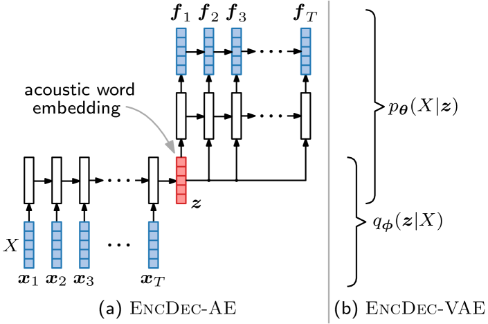
Fig. 1: The EncDec-AE is trained to predict its input (a speech segment) from the latent acoustic word embedding $\boldsymbol{{z}}$. The EncDec-VAE is a generative model which incorporates a prior over the latent acoustic embedding $\boldsymbol{{z}}$.

Taking together the above equations, the EncDec-VAE’s loss for a single training sequence $X$ is thus

$$\ell(X) =-\sum_{t=1}^{T}J_{t}(X)$$

$$=\sum_{t=1}^{T}\left[\frac{1}{2\sigma^{2}}\left|\left|\boldsymbol{{x}}_{t}-\boldsymbol{{f}}_{t}(\boldsymbol{{z}}^{\prime})\right|\right|^{2}+D_{\textrm{KL}}\left(q_{\boldsymbol{{\phi}}}(\boldsymbol{{z}}|X)||p(\boldsymbol{{z}})\right)\right]$$

This is a combination of a reconstruction term (as for the standard EncDec-AE) and a KL-regularisation term encouraging embedding $\boldsymbol{{z}}$ given input $X$ to be close to the prior distribution $p(\boldsymbol{{z}})$. The $\sigma$ hyperparameter controls the relative weight of reconstruction vs. regularisation. We use $\sigma={10}^{-5}$ (optimised in validation), so high emphasis is placed on reconstruction.

One motivation for the EncDec-VAE is that in the EncDec-AE we have empirically observed that embeddings for words of different types often take on very similar values across embedding dimensions. By specifying a prior, we obtain a handle on the spread or concentration of embedding values.

Fig. 2: An unsupervised term discovery system is used to obtain input-output speech segments for the encoder-decoder correspondence autoencoder (EncDec-CAE).

2.3 Encoder-decoder correspondence autoencoder

While the EncDec-AE uses the same speech segments as input and output, the encoder-decoder correspondence autoencoder (EncDec-CAE) uses weak top-down constraints in the form of discovered word pairs to have input and output sequences from different instances of the same predicted word type. This is illustrated in Figure 2. An unsupervised term discovery (UTD) system is applied to an unlabelled speech collection, discovering pairs of word segments predicted to be of the same type. These are then presented as input-output pairs to the EncDec-CAE. Since UTD is itself unsupervised, the overall approach is unsupervised.

For EncDec-CAE, a single training item consists of a pair of sequences $(X^{(a)},X^{(b)})$. Each segment consists of a unique sequence of frame-level vectors: $X^{(a)}=\boldsymbol{{x}}_{1}^{(a)},\ldots,\boldsymbol{{x}}_{T_{a}}^{(a)}$ and $X^{(b)}=\boldsymbol{{x}}_{1}^{(b)},\ldots,\boldsymbol{{x}}_{T_{b}}^{(b)}$. The loss for a single training pair is $\ell(X^{(a)},X^{(b)})=\sum_{t=1}^{T_{b}}||\boldsymbol{{x}}^{(b)}_{t}-\boldsymbol{{f}}_{t}(X^{(a)})||^{2}$, where $X^{(a)}$ is the input and $X^{(b)}$ the target output. We found that it is crucial to first pretrain the EncDec-CAE as a standard AE using the loss in §2.1, before switching to the loss here.

The correspondence idea is not new—its application in the encoder-decoder architecture is. In [31] it was used to improve frame-level rather than segmental speech representations. Earlier [32] and more recent work [33] in domains outside of speech have also used neighbours in the input feature space as model targets. Term discovery systems were also used to provide training segments for a speech model in [22]. Although their systems are unsupervised, the intrinsic quality of embeddings was not their direct focus, as is also the case in [11, 20]. Another study where ground truth segments are not used is [24], although true phoneme boundaries are assumed.

3 Experiments

3.1 Experimental setup and evaluation

We perform experiments on two languages, using the same data as in previous zero-resource studies [3]. English training, validation and test sets are obtained from the Buckeye corpus [34], each with around 6 hours of speech. For Xitsonga we use a 2.5 hour portion of the NCHLT corpus [35]. We use word pairs discovered using the UTD system of [36]. On the English training data, this system discovers around 14k unique pairs; on the Xitsonga data, it discovers around 6k pairs. For comparison, we also extract a similarly sized set of ground truth word segments from forced alignments of the English training data. All speech audio is parametrised as static Mel-frequency cepstral coefficients (MFCCs), i.e. $D=13$.

Ultimately we want to use acoustic embeddings downstream in zero-resource speech applications. But here we want to measure intrinsic quality without being tied to a particular system architecture. We therefore use a word discrimination task designed for this purpose [37]. In the same-different task, we are given a pair of acoustic segments, each a true word, and we must decide whether the segments are examples of the same or different words. To do this using an embedding method, a set of words in the test data (we use around 5k tokens in both languages) are embedded using the specific approach. For every word pair in this set, the cosine distance between their embeddings is calculated. Two words can then be classified as being of the same or different type based on some threshold, and a precision-recall curve is obtained by varying the threshold. The area under this curve is used as final evaluation metric, referred to as the average precision (AP).

As a baseline embedding method, we use downsampling by keeping 10 equally-spaced MFCC vectors from a segment with appropriate interpolation, giving a 130-dimensional embedding. This has proven a strong baseline in other work [24]. The same-different task can also be approached by using DTW alignment between test segments, where the alignment cost of the full sequences are used as a score for word discrimination.

All neural models are implemented in TensorFlow. For all models we use an embedding dimensionality of $M=\textrm{130}$, to be directly comparable to the downsampling baseline. More importantly, although other studies consider higher-dimensional settings, downstream systems such as [14] are constrained to embedding sizes of this order. Neural network architectures were optimised on the English validation data. Our final EncDec models all have 3 encoder and 3 decoder unidirectional RNN layers, each with 400-unit hidden representations. We also considered bidirectional RNNs, but this did not give improvements. Pairs are presented to the EncDec-CAE in both input-output directions. Models are trained using Adam optimisation [38] with a learning rate of 0.001. On the English data, early stopping is used, but for Xitsonga validation data is not available so the models are simply trained for 100 epochs. We run all models with five different initialisations and report average performance and standard deviations.

Table 1: Word discrimination performance on test data. UTD was used to provide training segments for the EncDec models.

	Average precision (%)
Model	English	Xitsonga
EncDec-AE	24.8 $\pm$ 0.50	14.2 $\pm$ 0.30
EncDec-VAE	25.0 $\pm$ 0.20	11.4 $\pm$ 0.40
EncDec-CAE	32.2 $\pm$ 0.01	32.0 $\pm$ 0.02
Downsampling	21.7	13.6
DTW alignment	35.9	28.1

3.2 Results

Table 1 shows AP performance on test data for all the neural embedding approaches, the downsampling baseline, and DTW alignment. All EncDec models here are trained on UTD segments, yielding truly unsupervised results. The dimensionalities of all the embeddings are also identical, $M=\textrm{130}$.

EncDec-CAE outperforms all other embedding approaches in both languages. In English it outperforms its closest competitor (EncDec-VAE) by roughly 29% relative in AP, while for Xitsonga it achieves more than twice the AP of EncDec-AE. In Xitsonga, EncDec-CAE also outperforms DTW, which has access to the full uncompressed sequences. This improvement is particularly notable since DTW is computationally more expensive: embedding comparisons with EncDec-CAE takes about 0.5 minutes on a single CPU core while DTW takes more than 60 minutes parallelised over 20 cores. In previous studies where embeddings were reported to outperform DTW, either ground truth word segments [18] or higher-dimensional embeddings were used [24].

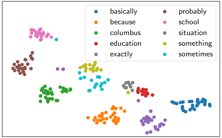
Fig. 3: t-SNE visualisations of acoustic word embeddings produced by EncDec-CAE on unseen data.

In Table 1, all EncDec models outperform downsampling apart from the Xitsonga EncDec-VAE. But downsampling is simple and does not require any training. In English, EncDec-VAE performs similar to EncDec-AE. This is not surprising since we had to weigh the reconstruction term in the VAE loss relatively high to obtain reasonable AP scores during validation. The poor performance in Xitsonga is in part due to the absence of a validation set: model hyperparameters (to which EncDec-VAE seem to be particularly sensitive) could not be tuned and early stopping was not possible. More work on EncDec-VAE is required to make definitive conclusions.

3.3 Further analysis

To quantify the penalty of using discovered instead of true word segments, Table 2 shows performance on the English validation data for the different EncDec models trained on different types of segments. The oracle column indicates AP when models are trained on ground truth word segments obtained from forced alignments. The random column shows AP when training segments are sampled randomly from within training utterances. EncDec-AE pays a small penalty when not using true segments, while EncDev-VAE performs best with UTD segments. EncDec-CAE cannot be trained on random segments as it requires paired data. When using perfect instead of discovered pairs, EncDec-CAE improves from 31.7% to 51.1% in AP. This is also the best overall performance on the English validation data—better than DTW. On the validation data here, downsampling yields performance similar to EncDec-AE and EncDec-VAE, without requiring any training segments. Row 3 shows that pretraining the EncDec-CAE is essential as performance drops considerably without it.

Figure 3 shows t-SNE visualisations [39] of embeddings from EncDec-CAE trained on UTD segments. Tokens of the same type are mapped to similar regions, and acoustically similar words such as ‘situation’ and ‘education’, or ‘something’ and ‘sometimes’ are located close to each other.

Table 2: Performance on English validation data, with models trained on ground truth, random and UTD segments.

	Average precision (%)
Model	Oracle	Random	UTD
EncDec-AE	26.2	25.5	25.7
EncDec-VAE	25.8	25.4	26.0
EncDec-CAE (non-init.)	46.9	-	19.0
EncDec-CAE	51.1	-	31.7
Downsampling	——  24.5  ——
DTW alignment	——  36.8  ——

4 Conclusion

We have evaluated old and new unsupervised neural acoustic word embedding methods for the truly unsupervised case where no word labels or boundaries are known. We showed that the encoder-decoder correspondence autoencoder (EncDec-CAE) outperforms other approaches in two languages. This model uses training pairs from a top-down unsupervised term discovery (UTD) system. When perfect segments are used, the EncDec-CAE also performs best and consistently outperforms a full alignment-based model. This indicates that the model could be even more effective given improvements in UTD accuracy. We also proposed the EncDec-VAE, a variational autoencoder over segments, but this model did not give improvements. It could, however, provide more explicit disentangled features [40], which we did not consider here and will investigate in future work.

References

- [1] G. Adda et al., “Breaking the unwritten language barrier: The BULB project,” Proc. SLTU, 2016.
- [2] A. Jansen et al., “A summary of the 2012 JHU CLSP workshop on zero resource speech technologies and models of early language acquisition,” in Proc. ICASSP, 2013.
- [3] M. Versteegh, X. Anguera, A. Jansen, and E. Dupoux, “The Zero Resource Speech Challenge 2015: Proposed approaches and results,” in Proc. SLTU, 2016.
- [4] E. Dunbar et al., “The Zero Resource Speech Challenge 2017,” in Proc. ASRU, 2017.
- [5] O. J. Räsänen, “Computational modeling of phonetic and lexical learning in early language acquisition: Existing models and future directions,” Speech Commun., vol. 54, pp. 975–997, 2012.
- [6] M. Elsner and C. Shain, “Speech segmentation with a neural encoder model of working memory,” in Proc. EMNLP, 2017.
- [7] A. S. Park and J. R. Glass, “Unsupervised pattern discovery in speech,” IEEE Trans. Audio, Speech, Language Process., vol. 16, no. 1, pp. 186–197, 2008.
- [8] T. J. Hazen, W. Shen, and C. White, “Query-by-example spoken term detection using phonetic posteriorgram templates,” in Proc. ASRU, 2009.
- [9] Y. Zhang and J. R. Glass, “Unsupervised spoken keyword spotting via segmental DTW on Gaussian posteriorgrams,” in Proc. ASRU, 2009.
- [10] K. Levin, A. Jansen, and B. Van Durme, “Segmental acoustic indexing for zero resource keyword search,” in Proc. ICASSP, 2015.
- [11] Y.-H. Wang, H.-y. Lee, and L.-s. Lee, “Segmental audio word2vec: Representing utterances as sequences of vectors with applications in spoken term detection,” in Proc. ICASSP, 2018.
- [12] C.-y. Lee, T. O’Donnell, and J. R. Glass, “Unsupervised lexicon discovery from acoustic input,” Trans. ACL, vol. 3, pp. 389–403, 2015.
- [13] O. J. Räsänen, G. Doyle, and M. C. Frank, “Unsupervised word discovery from speech using automatic segmentation into syllable-like units,” in Proc. Interspeech, 2015.
- [14] H. Kamper, K. Livescu, and S. Goldwater, “An embedded segmental k-means model for unsupervised segmentation and clustering of speech,” in Proc. ASRU, 2017.
- [15] S. Bhati, S. Nayak, and K. S. R. Murty, “Unsupervised speech signal to symbol transformation for zero resource speech applications,” in Proc. Interspeech, 2017.
- [16] L. R. Rabiner, A. E. Rosenberg, and S. E. Levinson, “Considerations in dynamic time warping algorithms for discrete word recognition,” IEEE Trans. Acoust., Speech, Signal Process., vol. 26, no. 6, pp. 575–582, 1978.
- [17] A. L. Maas, S. D. Miller, T. M. O’Neil, A. Y. Ng, and P. Nguyen, “Word-level acoustic modeling with convolutional vector regression,” in Proc. ICML Workshop Representation Learn., 2012.
- [18] K. Levin, K. Henry, A. Jansen, and K. Livescu, “Fixed-dimensional acoustic embeddings of variable-length segments in low-resource settings,” in Proc. ASRU, 2013.
- [19] Y.-A. Chung, C.-C. Wu, C.-H. Shen, and H.-Y. Lee, “Unsupervised learning of audio segment representations using sequence-to-sequence recurrent neural networks,” in Proc. Interspeech, 2016.
- [20] K. Audhkhasi, A. Rosenberg, A. Sethy, B. Ramabhadran, and B. Kingsbury, “End-to-end ASR-free keyword search from speech,” IEEE J. Sel. Topics Signal Process., vol. 11, no. 8, pp. 1351–1359, 2017.
- [21] S. Settle, K. Levin, H. Kamper, and K. Livescu, “Query-by-example search with discriminative neural acoustic word embeddings,” in Proc. Interspeech, 2017.
- [22] Y.-A. Chung, W.-H. Weng, S. Tong, and J. R. Glass, “Unsupervised cross-modal alignment of speech and text embedding spaces,” in Proc. NIPS, 2018.
- [23] Y.-A. Chung and J. R. Glass, “Speech2vec: A sequence-to-sequence framework for learning word embeddings from speech,” in Proc. Interspeech, 2018.
- [24] N. Holzenberger, M. Du, J. Karadayi, R. Riad, and E. Dupoux, “Learning word embeddings: unsupervised methods for fixed-size representations of variable-length speech segments,” in Proc. Interspeech, 2018.
- [25] Y.-C. Chen, S.-F. Huang, C.-H. Shen, H.-y. Lee, and L.-s. Lee, “Phonetic-and-semantic embedding of spoken words with applications in spoken content retrieval,” in Proc. SLT, 2018.
- [26] K. Cho et al., “Learning phrase representations using RNN encoder-decoder for statistical machine translation,” in Proc. EMNLP, 2014.
- [27] A. Sperduti and A. Starita, “Supervised neural networks for the classification of structures,” IEEE Trans. Neural Netw., vol. 8, no. 3, pp. 714–735, 1997.
- [28] J. Chung, C. Gulcehre, K. Cho, and Y. Bengio, “Empirical evaluation of gated recurrent neural networks on sequence modeling,” arXiv preprint arXiv:1412.3555, 2014.
- [29] D. P. Kingma and M. Welling, “Auto-encoding variational bayes,” arXiv preprint arXiv:1312.6114, 2013.
- [30] C. Doersch, “Tutorial on variational autoencoders,” arXiv preprint arXiv:1606.05908, 2016.
- [31] D. Renshaw, H. Kamper, A. Jansen, and S. J. Goldwater, “A comparison of neural network methods for unsupervised representation learning on the Zero Resource Speech Challenge,” in Proc. Interspeech, 2015.
- [32] C. Silberer and M. Lapata, “Learning grounded meaning representations with autoencoders,” in Proc. ACL, 2014.
- [33] T. B. Hashimoto, P. S. Liang, and J. C. Duchi, “Unsupervised transformation learning via convex relaxations,” in Proc. NIPS, 2017.
- [34] M. A. Pitt, K. Johnson, E. Hume, S. Kiesling, and W. Raymond, “The Buckeye corpus of conversational speech: Labeling conventions and a test of transcriber reliability,” Speech Commun., vol. 45, no. 1, pp. 89–95, 2005.
- [35] N. J. De Vries et al., “A smartphone-based ASR data collection tool for under-resourced languages,” Speech Commun., vol. 56, pp. 119–131, 2014.
- [36] A. Jansen and B. Van Durme, “Efficient spoken term discovery using randomized algorithms,” in Proc. ASRU, 2011.
- [37] M. A. Carlin, S. Thomas, A. Jansen, and H. Hermansky, “Rapid evaluation of speech representations for spoken term discovery,” in Proc. Interspeech, 2011.
- [38] D. Kingma and J. Ba, “Adam: A method for stochastic optimization,” in Proc. ICLR, 2015.
- [39] L. Van der Maaten and G. Hinton, “Visualizing data using t-SNE,” J. Mach. Learn. Res., vol. 9, no. Nov, pp. 2579–2605, 2008.
- [40] W.-N. Hsu, Y. Zhang, and J. R. Glass, “Unsupervised learning of disentangled and interpretable representations from sequential data,” in Proc. NIPS, 2017.