Encoding and Visualization in the Collatz Conjecture

Abstract

The Collatz conjecture is one of the easiest mathematical problems to state and yet it remains unsolved. For each $n\geq 2$ the Collatz iteration is mapped to a binary sequence and a corresponding unique integer which can recreate the iteration. The binary sequence is used to produce the Collatz curve, a 2-D visualization of the iteration on a grid, which, besides the aesthetics, provides a qualitative way for comparing iterations. Two variants of the curves are explored, the r-curves and on-change-turn-right curves. There is a scarcity of acyclic r-curves and only three r-curves were found having a cycle of minimum length greater than 4.

I Introduction

The Collatz Conjecture states that starting with a positive integer $n$, the iteration of the function

$$C(n)=\begin{cases}\frac{n}{2},&\text{if $n\equiv 0\pmod{2}$}\\ 3n+1,&\text{if $n\equiv 1\pmod{2}$,}\end{cases}$$ (1)

eventually reaches 1; that is to say that there exists a finite integer $k$ such that $C^{k}(n)=1$. For example, starting with $n=3$, $C^{0}(3)=3$, we obtain the sequence $3\rightarrow 10\rightarrow 5\rightarrow 16\rightarrow 8\rightarrow 4\rightarrow 2\rightarrow 1$. Continuing the iteration, it is noted that the sequence is caught in the cycle $1\rightarrow 4\rightarrow 2\rightarrow 1$. The Collatz conjecture can be stated in another way: starting the iteration with any positive integer $n$ there is no other cycle than this one and the iteration does not diverge to infinity.

The origins of the Collatz Conjecture can be traced back to the 1930’s to the German mathematician Luther Collatz [1]. Although known in the 1950’s among mathematicians, it first appeared in print in 1971 [2, 1]. Despite the simplicity with which it can be stated and despite the multitude of mathematicians who studied it and attempted to solve it, its proof has remained elusive. Empirically, it has been verified to be true for $n<5\times 2^{60}\approx 5.7646\times 10^{18}$ [3].

The consensus seems to be that a proof is not within reach at this time. In general, randomness and unpredictability govern the sequences produced by the iterations from one number to the next. Paul Erdős famously commented “Mathematics may not be ready for such problems” [1]. The conjecture, as it circulated in many campuses through many mathematicians, it came to be known by various names such as the $3x+1$ problem, the Syracuse Problem, Hasse’s Algorithm, Kakutani’s Problem and Ulam’s Problem [1, 4]. The sequence of numbers produced by the Collatz iteration is known as hailstone numbers [5].

It is noted that in Equation 1, when the second rule is applied, the resulting number $3n+1$ is necessarily an even number, and hence the iteration can be written more compactly thusly [6, 7, 1]:

$$T(n)=\begin{cases}\frac{n}{2},&{\text{if $n\equiv 0\pmod{2}$}}\\ \frac{3n+1}{2},&{\text{if $n\equiv 1\pmod{2}$.}}\end{cases}$$ (2)

This version of the iteration is widely used and it will be used for the rest of this paper. Using the same example $n=3$, with iteration $T^{k}(n)$ the sequence produced is $3\rightarrow 5\rightarrow 8\rightarrow 4\rightarrow 2\rightarrow 1$, and the cycle becomes $1\rightarrow 2\rightarrow 1$.

The total stopping time $\sigma_{\infty}(n)$ of $n$ is the least $k$ applications of $T$ that the sequence of the iteration will reach 1 for the first time:

$$\sigma_{\infty}(n)=\inf\>\{k:T^{k}(n)=1\}.$$ (3)

For example, $\sigma_{\infty}(3)=5.$

In this paper, the iteration $T^{k}(n)$ of each number $n$ is encoded as a binary number (or string), and in turn as a unique positive integer $m$. The binary string is mapped to a curve in 2-D in an analogous way that the binary string of the Dragon Curve is mapped to the corresponding curve.

II The Binary Encoding

The conversion of a decimal number $n$ to its corresponding binary representation involves successive divisions by 2 and looking at the parity of the result. We note that the process is similar to the Collatz iteration: each time $T(n)$ is applied a decision is made based on whether $n$ is even or odd. We choose to have a “1” if $T^{k}(n)$ is even and “0” if odd. For example, $n=3$ is encoded as 11100. The bits are produced, just like in the usual decimal-to-binary conversion, from right to left. Table I shows the binary encoding and decimal equivalent.

For all $n\geq 2$, assuming that the Collatz Conjecture is true, the last application of $T$ is on $2$, an even number, before reaching $1$. Making the same assumption, the binary encoding of all $n\geq 5$ begins with $111$, noting that eventually the iteration will end with $8\rightarrow 4\rightarrow 2\rightarrow 1$. The length of the binary encoding of $n$ is $\sigma_{\infty}(n)$ since the number of digits is exactly the number of applications of $T$ needed to reach $1$ in the sequence of iterations. The choice of when to use “1” or “0” was made so that the binary encoding of $n$, the original number, starts with a “1”, to avoid having any leading zeros. Had we had any leading zeros, the binary string would not have been recoverable from its corresponding decimal number, since leading zeros are not significant and are ignored when converting to decimal. This sequence was independently published as sequence A304715 in OEIS [8], which we noticed after a draft of this paper had been released.

Given the binary encoding of $n$, it is a simple matter to find the original $n$. It can be done by the following process: Scan its binary encoding $B=b_{l}b_{l-1}\ldots{}b_{1}b_{0}$, where $b_{l}$ is the most significant bit, from left to right. Starting with initial $n=1$ and $i=0$, iteratively apply $R^{i}(n,b)$, for $i=0,1,\ldots,l$:

$$R^{i}(n,b)=\begin{cases}2n,&{\text{if $b_{l-i}=1$}}\\ \frac{2n-1}{3},&{\text{if $b_{l-i}=0$}}.\end{cases}$$ (4)

As an example, given the encoding $B=11100$, starting with $n=1$ and iteratively applying $R^{i}(n,b)$ we obtain the sequence $1\rightarrow 2\rightarrow 4\rightarrow 8\rightarrow 5\rightarrow 3$, and thus we obtain $n=3$. This is the reverse sequence produced by Equation 2.

$n$	Binary encoding	Decimal
2	1	1
3	11100	28
4	11	3
5	1110	14
6	111001	57
7	11101101000	1896
8	111	7
9	1110110100010	7586
10	11101	29
11	1110110100	948
12	1110011	115
13	1110110	118
14	111011010001	3793
15	111011110000	3824
16	1111	15
17	111011010	474
18	11101101000101	15173
19	11101101001100	15180
20	111011	59
21	111110	62
22	11101101001	1897
23	11101111000	1912
24	11100111	231
25	1110110100110010	60722
26	11101101	237
27	111011110001101110 101011100001100000 010010001101000010   010010010100000100	1102691417057682138372
28	1110110100011	7587
29	1110110100110	7590
30	1110111100001	7649

TABLE I: The binary and corresponding decimal encoding.

III Collatz Curves: Visualizing the Binary Encoding

For each positive integer $n\geq 2$, we will visualize the Collatz sequence generated by the iteration $T^{k}(n)$ by making use of its binary encoding (Table I). The binary encoding is viewed as a random walk where each of its digits generates a unit length line segment in a certain direction.

The manner of generating the Collatz curve corresponding to $n$ is similar to that of generating the Dragon Curve (Figure 1) [9, 10].

Figure 1: The Dragon Curve of order $10$.

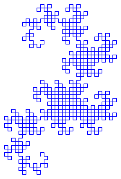
The string $S_{k}$ of the Dragon Curve of order $k$ is generated as follows. There are two symbols, R (right) and L (left). In the first iteration (order $k=1$) the string $S_{1}$ is just the symbol R. In each successive iteration the new string $S_{n+1}$ is recursively produced:

$$S_{n+1}=S_{n}+R+\overline{S}_{n},$$ (5)

where $+$ is string concatenation and $\overline{S}_{n}$ is $S_{n}$ reversed with each of its symbols flipped. Table II shows the first four iterations.

Iteration ($k$)	String $S_{k}$
1	R
2	R R L
3	R R L R R L L
4	R R L R R L L R R R L L R L L

TABLE II: The first four iterations of the Dragon Curve.

Let $S_{k}=s_{l}s_{l-1}\ldots s_{1}s_{0}.$ From $S_{k}$ a curve can be produced such as the one in Figure 1 ($k=10$) by making use of turtle graphics [11, 12]: string $S_{k}$ is scanned from left to right:

if $s_{i}=R$,	turn right $90^{\circ}$, move forward one unit
if $s_{i}=L$,	turn left $90^{\circ}$, move forward one unit.

The initial orientation of the turtle in all figures in this paper is facing east.

The curve of each Collatz sequence is produced in an analogous way. The digits of the binary encoding $B$ of $n$ are scanned from right to left.

if $b_{i}=1$,	turn right $90^{\circ}$, move forward one unit
if $b_{i}=0$,	turn left $90^{\circ}$, move forward one unit.

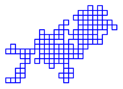
The curve for $n=3$ appears in Figure 2. Its binary encoding is $11100$. The initial point, that is the initial position of the turtle, is at the bottom of the curve. A more involved curve is generated for $n=27$ (Figure 3), a number known for its relatively long binary encoding, which is of length $70$. A still more involved curve, for $n=75,128,138,247$, is shown in Figure 4, which bears a resemblance of the figure of a lion. Its binary sequence is of length $767$.

Figure 2: The curve for $n=3$.

Figure 3: The curve for $n=27$.

Figure 4: The “lion curve” for $n=75,128,138,247$.

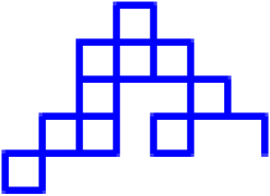
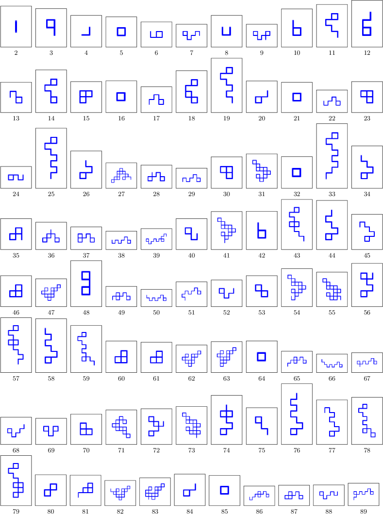
The curve for $n=6$ (Figure 5, also in Figure 11), whose binary encoding is $111001$, coincidentally forms the shape of $6$! The orientation is arbitrary since it only depends on the starting orientation of the turtle.

Figure 5: The curve for $n=6$.

Figure 11 shows the Collatz curves for $2\leq n\leq 89$ and Figure 12 those for $90\leq n\leq 177$.

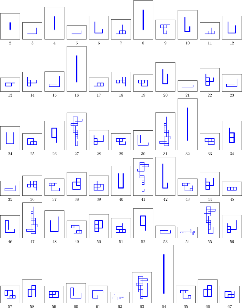
One important difference between the Dragon Curve and the curves we generate using the Collatz iteration is the former does not intersect itself [9], whereas the latter ones do. It is possible, and it often happens, that the curve as it is generated writes over previously generated segments. Hence, although the binary encoding is unique for each $n$, as discussed in Section II, its corresponding curve is not. As an example, the curves for $n=2^{k},k\geq 4$ appear identical: a unit square, which can be seen in Figures 11 and 12 for $n=16,32,64,128.$ But powers of two are not the only ones that produce a square, e.g. consider the figures of $n=5,21,85.$

Theorem 1

Assuming that the Collatz Conjecture is true, all curves for $n\geq 2$, except those for $n=2,4,\text{or }8$, end with a cycle, i.e. a unit square.

Proof:

For $n=2,4,8$ the binary encoding is of length three or less (Table I), which precludes forming a cycle, since a cycle requires at least 4 segments. For all other $n$ the binary encoding is of length 4 or more and the iteration ends in the cycle $4\rightarrow 2\rightarrow 1$. Necessarily, the sequence before reaching $1$ for the first time is $8\rightarrow 4\rightarrow 2\rightarrow 1$, which corresponds to $111$. Right before $111$ is drawn, the turtle is at the end of an existing segment. Turning right and drawing 3 times creates a final cycle. ∎

Definition 1

The girth $g(G)$ of a graph $G$ is the minimum length of a cycle contained in $G$ [13]. If $G$ has no cycles, $g(G)=\infty$.

Corollary 1

When the Collatz curve is viewed as a graph $G(n)=(V,E)$, $g(G(n))=4$ for all $n>8$.

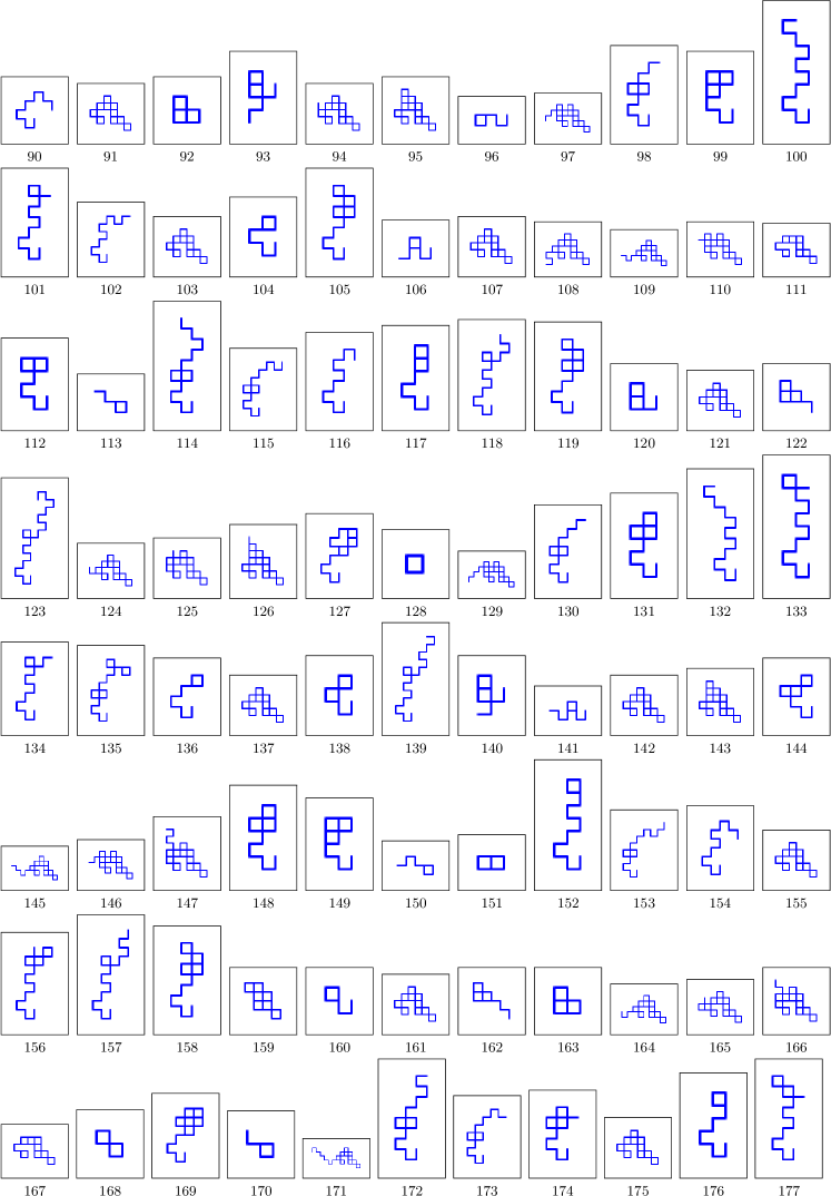
The curves allow for easy identification of similar patterns in the Collatz iteration. As an example, visually inspecting the curves in Figure 11, we note that those for $n=27$, $31$, $41$, $47$, $54$, $55$, $62$, $63$, $71$, $73$, $82$, and $83$ bear a strong resemblance to each other. A closer look at the binary encodings reveals that indeed when compared pairwise they have a long common substring (subsequence). Table III shows the lengths of the longest common substrings, all of which happen to start from the leftmost bit position (see Table IV). Each common substring is of length at least 60. In Table III, on the diagonal is the length of the binary encoding of the corresponding $n$.

	27	31	41	47	54	55	62	63	71	73	82	83
27	70	67	69	66	70	66	68	60	65	66	69	66
31	67	67	67	66	67	66	67	60	65	66	67	66
41	69	67	69	66	69	66	68	60	65	66	69	66
47	66	66	66	66	66	66	66	60	65	66	66	66
54	70	67	69	66	71	66	68	60	65	66	69	66
55	66	66	66	66	66	71	66	60	65	71	66	70
62	68	67	68	66	68	66	68	60	65	66	68	66
63	60	60	60	60	60	60	60	68	60	60	60	60
71	65	65	65	65	65	65	65	60	65	65	65	65
73	66	66	66	66	66	71	66	60	65	73	66	70
82	69	67	69	66	69	66	68	60	65	66	70	66
83	66	66	66	66	66	70	66	60	65	70	66	70

TABLE III: The pairwise length of the longest common substring of the binary encodings. On the diagonal is the length of the binary encoding of the corresponding $n$.

n	Binary encoding
27	1110111100011011101010111000011000000100100011010000100010010100000100
31	1110111100011011101010111000011000000100100011010000100010010100000
41	111011110001101110101011100001100000010010001101000010001001010000010
47	111011110001101110101011100001100000010010001101000010001001010000
54	11101111000110111010101110000110000001001000110100001000100101000001001
55	11101111000110111010101110000110000001001000110100001000100101000011000
62	11101111000110111010101110000110000001001000110100001000100101000001
63	11101111000110111010101110000110000001001000110100001000100111000000
71	11101111000110111010101110000110000001001000110100001000100101000
73	1110111100011011101010111000011000000100100011010000100010010100001100010
82	1110111100011011101010111000011000000100100011010000100010010100000101
83	1110111100011011101010111000011000000100100011010000100010010100001100

TABLE IV: Numbers with similar binary encodings, i.e. similar trajectories in the Collatz iteration. They have been identified visually via their Collatz curves. Pairwise they have a common substring, leftmost bits, of length at least 60. The 60th bit from the left is in bold.

IV Reverse Curves

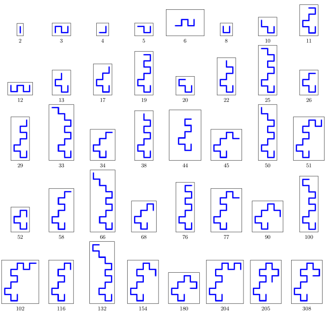
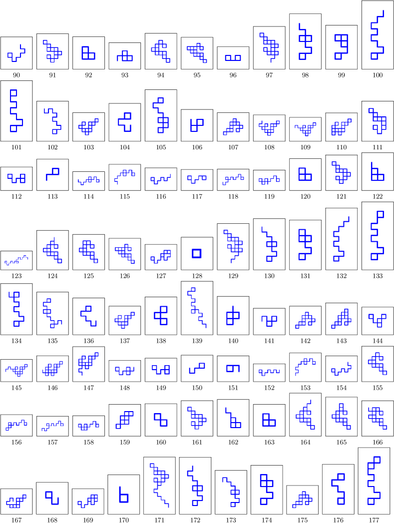
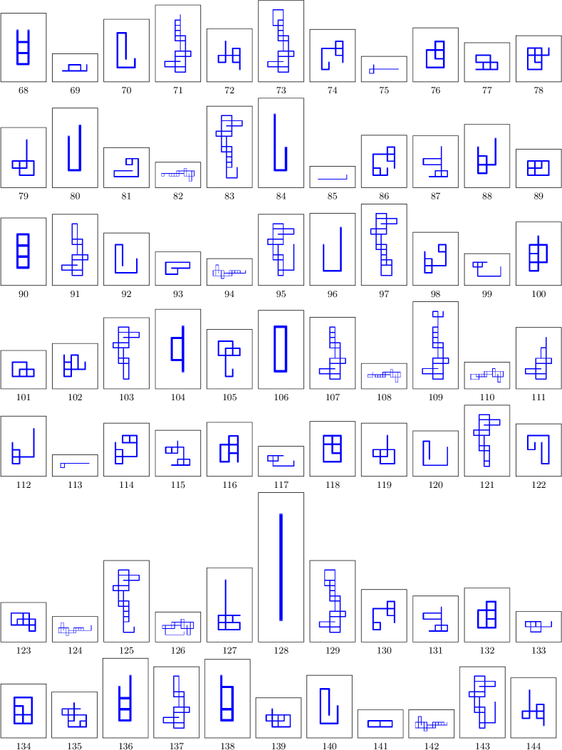
Another version of the Collatz curves can be obtained by applying the same rules except that the bits in the encoding of $n$ are scanned in reverse, from left-to-right. The resulting reverse curves, or r-curves, are very similar to the Collatz curves. In general they are not affine transformations of each other. Theorem 1 does not apply, and thus the curves no longer necessarily have a cycle for $n>8$. As an example, compare the two curves for $n=33$ in Figure 6. The r-curve has no cycle. Figure 13 shows the r-curves for $2\leq n\leq 89$ and Figure 14 those for $90\leq n\leq 177$.

                 

Figure 6: For $n=33$, the Collatz curve (left) and the r-curve (right). Note the absence of a cycle in the r-curve.

Two questions arise: (1) how many r-curves are devoid of cycles, and (2) how many r-curves have finite girth $g(G(n))>4$, i.e. they have a cycle of minimum length other than the unit square. Using Python 3 and the software library NetworkX [14], we have checked all r-curves up to $n\leq 10^{8}$ and we found that there are only 40 r-curves with no cycles, with the largest $n=308$. All such curves can be found in Figure 10.

In the same range, i.e. up to $n\leq 10^{8}$, it was found that there are only three r-curves having finite girth $g(G(n))>4$, and those are for $n=273,410,\text{and }820$. In all three cases $g(G(n))=12$. The only cycle in these curves is the cross pattern which can be seen in Figure 7. We call these curves miracle curves. The ones for $410$ and $820$ are identical due to overwriting.

(a) 273

(b) 410

(c) 820

Figure 7: Miracle curves: The only three r-curves found having a cycle of minimum length greater than $4$, verified up to $n\leq 10^{8}$. Their only cycle, the cross pattern, has length $12$. The curves for $410$ and $820$ are identical due to overwriting.

V Alternative Curves

It is possible to use alternative schemes to draw the curves that correspond to the binary encoding of $n$ by modifying the rules. For example, we can use this rule for the turtle:

if $b_{i}=b_{i-1}$,	move forward one unit
if $b_{i}\neq b_{i-1}$,	turn right $90^{\circ}$, move forward one unit.

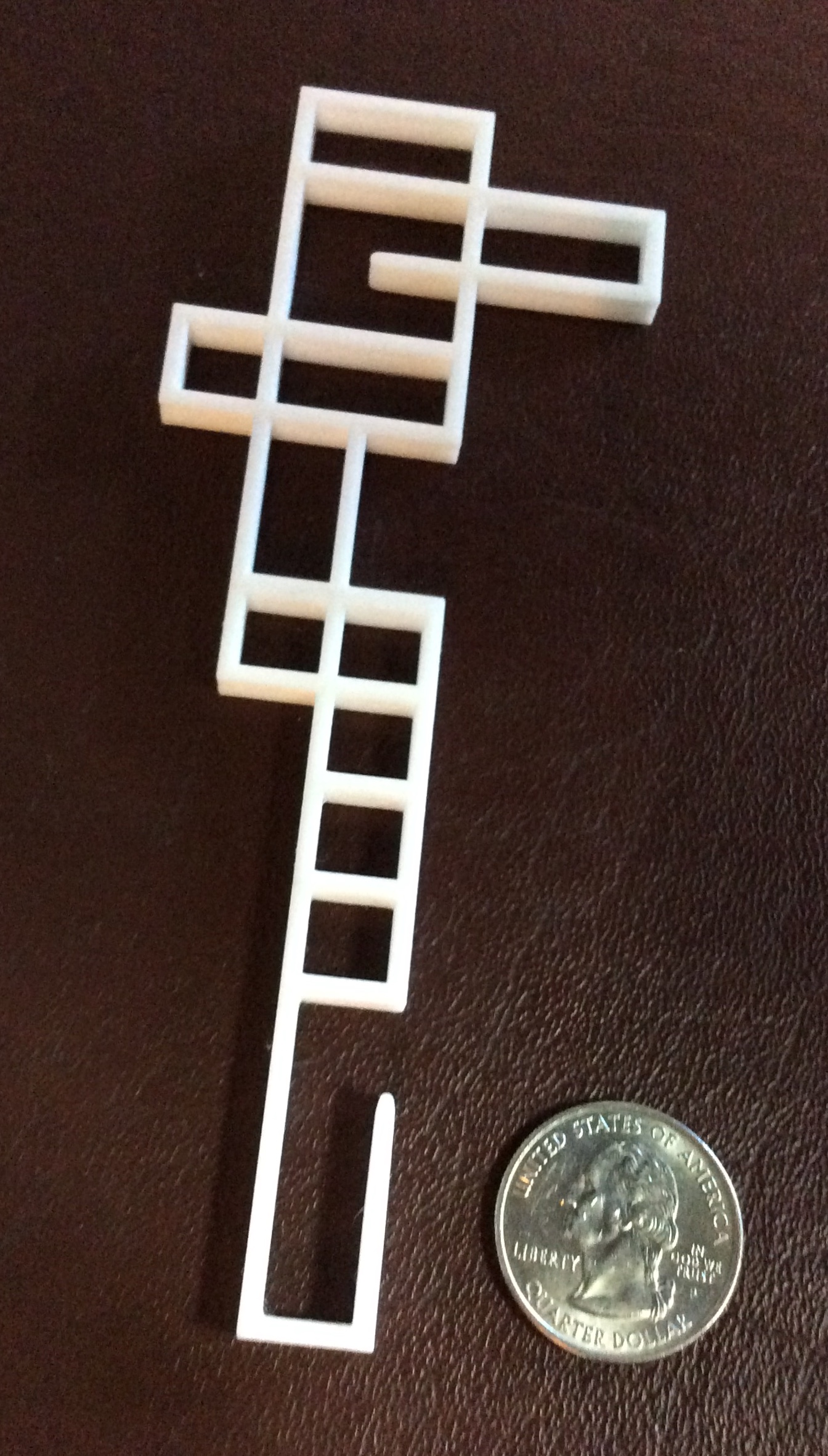
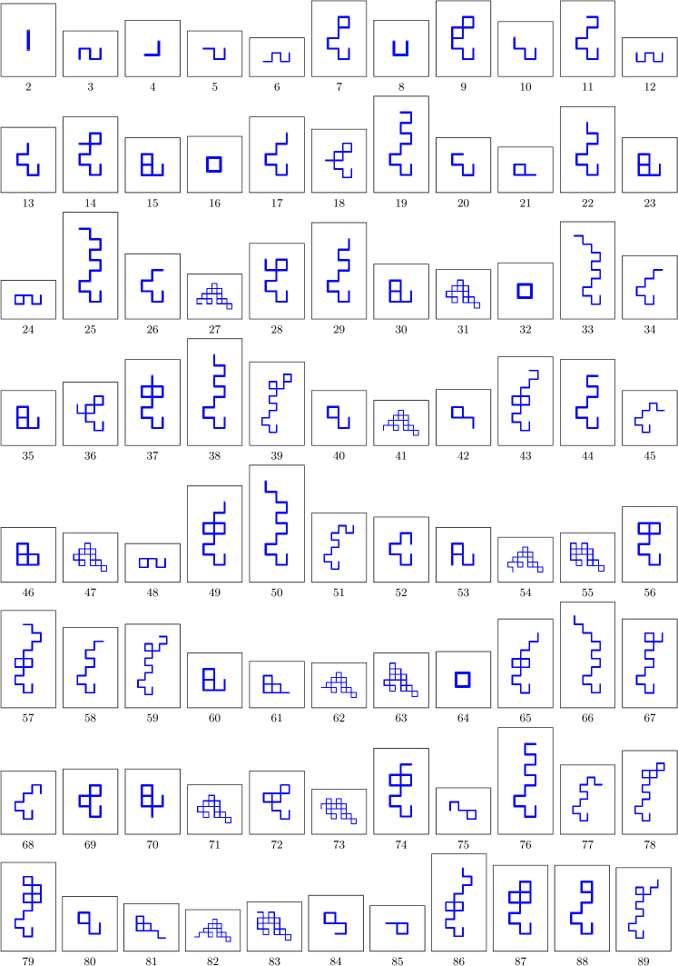
In other words, as long as there is no change from one bit to the next, scanning the bits from right to left, either from 0 to 1 or vice versa, the turtle keeps moving forward. If there is a change, the turtle turns right $90^{\circ}$ and moves forward. The on-change-turn-right curves produced with this rule appear in Figures 15 and 16. Visual identification of similar curves, e.g. those similar to the curve of $n=27$, is easily done. These curves are characterized by longer straight lines compared to the Collatz curves, Figures 11 and 12. For comparison with Figure 3, the on-change-turn-right curve for $n=27$ is shown in Figure 8. For purely aesthetic reasons, we show the picture of the same curve 3-D printed in Figure 9.

Figure 8: The on-change-turn-right curve for $n=27$.

Figure 9: The on-change-turn-right curve for ${n=27}$ 3-D printed.

VI Conclusion

Figure 10: The r-curves without cycles. Verified up to $n\leq 10^{8}$.

The Collatz iteration for each $n\geq 2$ is mapped to a binary sequence, which in turn is mapped to an integer. The binary sequence is translated to a 2-D curve on a grid, the Collatz curve, in an analogous way that the Dragon Curve is drawn from a binary sequence. Two variants of the curves were explored: the reverse curves (r-curves) and the the on-change-turn-right curves. There is a scarcity of acyclic r-curves, only 40 were found, and only three r-curves were found having a shortest length cycle of length greater than four, the miracle curves. This was verified up to $n\leq 10^{8}$. The Collatz curves, the r-curves, and the on-change-turn-right curves provide a way to visualize and qualitatively compare Collatz iterations.

References

- [1] J. C. Lagarias, “The 3x + 1 problem and its generalizations,” The American Mathematical Monthly, vol. 92, pp. 3–23, 1 1985.
- [2] H. Coxeter, “Cyclic sequences and frieze patterns,” Vinculum, vol. 8, pp. 4–7, 1971.
- [3] T. Oliveira e Silva, “Empirical verification of the and related conjectures,” in The Ultimate Challenge: The Problem (J. C. Lagarias, ed.), pp. 189–207, Providence, Rhode Island, USA: American Mathematical Society, 2010.
- [4] J. C. Lagarias, “The 3x+1 problem: An annotated bibliography, II (2000-2009).” arXiv:math/0608208, 2011.
- [5] B. Hayes, “Computer recreations: The ups and downs of hailstone numbers,” Scientific American, vol. 250, no. 1, pp. 10–16, 1984.
- [6] R. Terras, “A stopping time problem on the positive integers,” Acta Arithmetica, vol. 3, no. 30, pp. 241–252, 1976.
- [7] R. Terras, “On the existence of a density,” Acta Arithmetica, vol. 35, pp. 101–102, 1979.
- [8] R. Sigrist, “The On-Line Encyclopedia of Integer Sequences.” A304715, May 2018.
- [9] C. Davis and D. E. Knuth, “Number representations and dragon curves,” Journal of recreational Mathematics, vol. 3, no. 2, pp. 66–81, 1970.
- [10] M. Gardner, Mathematical magic show: more puzzles, games, diversions, illusions and other mathematical sleight-of-mind from Scientific American, pp. pages 207–209 and 215–220. Vintage, 1978.
- [11] H. Abelson and A. A. DiSessa, Turtle geometry: The computer as a medium for exploring mathematics. Cambridge, Mass: MIT Press, 1986.
- [12] “Heighway’s Dragon Curve using Python.” https://www.geeksforgeeks.org/heighways-dragon-curve-python/. Accessed = 2018-10-9.
- [13] R. Diestel, Graph theory. Springer, fifth edition ed., 2017.
- [14] A. A. Hagberg, D. A. Schult, and P. J. Swart, “Exploring network structure, dynamics, and function using NetworkX,” in Proceedings of the 7th Python in Science Conference (G. Varoquaux, T. Vaught, and J. Millman, eds.), (Pasadena, CA), pp. 11–15, 2008.