Stability of Quantum Dynamics under Constant Hamiltonian Perturbations

Abstract

Concepts like “typicality” and the “eigenstate thermalization hypothesis” aim at explaining the apparent equilibration of quantum systems, possibly after a very long time. However, these concepts are not concerned with the specific way in which this equilibrium is approached. Our point of departure is the (evident) observation that some forms of the approach to equilibrium, such as, e.g., exponential decay of observables, are much more common then others. We suggest to trace this dominance of certain decay dynamics back to a larger stability with respect to generic Hamiltonian perturbations. A numerical study of a number of examples in which both, the unperturbed Hamiltonians as well as the perturbations are modelled by partially random matrices is presented. We furthermore develop a simple heuristic, mathematical scheme that describes the result of the numerical investigations remarkably well. According to those investigations the exponential decay indeed appears to be most stable. Dynamics that are in a certain sense at odds with the arrow of time are found to be very unstable.

I Introduction

While it is an empirical fact that closed (quantum) systems with many degrees of freedom (e.g. a solid initially prepared with some temperature-inhomogeneities, insulated from the rest of the world) in some sense equilibrate, the question how such equilibration-processes emerge from the (reversible, non-chaotic) microscopic principles of quantum-mechanics is still under debate. Accordingly, the eventual occurrence of equilibrium, has been investigated with great efforts, even and especially during the last decades Gogolin and Eisert (2016). But recently also the specific way into the equilibrium-state Niemeyer et al. (2013a), the relaxation timescales of expectation values García-Pintos et al. (2017) as well as the stability of equilibrium states Farrelly et al. (2017) have gathered growing attention. A central aspect of the route to equilibrium is irreversibility. In this context, additional to mere Loschmidt echos Peres (1984), alternative indicators have lately been employed to quantify the stability of the dynamics against small, time-local perturbations Larkin and Ovchinnikov (1969); Schmitt and Kehrein (2017). These indicators are based on observables, which are accessible in experiment Swingle et al. (2016); Campisi and Goold (2017). The typical form of the full relaxation dynamics of an observable the eigenstates of which are entirely unrelated to an respective Hamiltonian, has been analyzed in Ref. Reimann (2016), finding that this type of observable practically always relaxes much more quickly than many practical physical observables do. Thus, the question in which sense general principles, that appear to apply to the route to equilibrium for almost all practical observables, emerge from the underlying quantum dynamics, remains open.

In the paper at hand, similar to Ref. Reimann (2016), we also consider observables the matrix elements of which are to some extend drawn at random w.r.t the eigenbasis of some Hamiltonian. However, in order to address the large class of practically occurring, slower relaxations, we specifically restrict the randomness: We construct pairs of Hamiltonians and observables $H_{0},A$ such that $\langle A(t)\rangle$ conforms with a predefined (slow) “relaxation function” $g(t)$, i.e.,

$$\langle A(t)\rangle\approx\langle A(0)\rangle g(t),$$ (1)

for initial states to be specified below. Within the limit set by condition (1), $H_{0},A$ are chosen as “random as possible”, see Sect. II. This construction of $H_{0},A$ serves as a basis to analyze if and how $\langle A(t)\rangle$ changes upon the addition of a perturbation $V$ to $H_{0}$, see Sect. IV. The perturbation $V$ is also modeled by a partially random matrix featuring some structure to account for physically plausibility, see Sect. III. If $\langle A(t)\rangle$ does not (or only negligibly) change due to the perturbation we call the respective $g(t)$ stable. Note that $\langle A(t)\rangle$ may remain stable, even though the perturbation possibly changes the evolution of the density matrix itself substantially (cf. Fig. 1). Our central question is whether or not stable relaxation dynamics coincide with those observed frequently in nature. Such a coincidence (for which we present evidence in Sect. IV) hints in the direction of rare relaxation dynamics being rare due to their instability. In Sect. V we develop a simple heuristic scheme which describes the effect of the perturbation on $\langle A(t)\rangle$ quite accurately. This model also supports the instability of “unusual” relaxation dynamics. These findings also relate to the concept of an “arrow of time”: Consider a $\langle A(t)\rangle$ which is at odds with the arrow of time due to a large recurrence, such as, e.g.

$$\langle A(t)\rangle=\exp(-{\frac{t}{\tau}})+\frac{1}{2}\exp(-{\frac{|t-T|}{\tau}})\quad t>0,T\gg\tau.$$ (2)

Note that the example (2) is unrelated to a (quasi-) Poincare recurrence, since the recurrence does not appear periodically. Note furthermore that this concept of a violation of the arrow of time differs conceptually from the one discussed in, e.g., Ref. Jennings and Rudolph (2010). The recurrence dynamics (2) is fully compatible with the quantum “non-resonance” equilibration principles suggested, e.g., in Refs. Reimann (2008); Short (2011); Lychkovskiy (2010)). It may furthermore occur for “non-fine tuned” initial states and is not at odds with the eigenstate thermalization hypothesis, as will be explained in Sect. II. However, dynamics of this type are hardly ever encountered in nature Within our approach this is traced back to their instability, see Sect. VI

II Construction of main Hamiltonian and Observable

In this Sect. we describe and motivate the scheme used to construct pairs of Hamiltonians and observables $H_{0},A$ in order to fulfill Eq. (1). However, we start by elaborating on our choice of initial states.

We focus on initial states which relate to the observables as

$$\rho(t=0)=\frac{\Pi_{E}(1+\delta\mathcal{A})\Pi_{E}}{\mathrm{Tr}(\Pi_{E}(1+\delta\mathcal{A}))}$$ (3)

with $\delta$ sufficiently small to render $\rho$ positive. $\Pi_{E}$ denotes a projector projecting onto a (possibly small) energy window of some Hamiltonian $\mathcal{H}_{0}$, the latter is to be defined below. From the point of view of linear response (3) may be viewed as a “response state”, state generated by the application of a weak static stimulus of the form $\mathcal{A}$ to an equilibrium state that essentially lives on the energy shell spanned by $\Pi_{E}$ Toda et al. (2012); Bartsch and Gemmer (2017). (For simplicity of notation we define $A:=\Pi_{E}\mathcal{A}\Pi_{E}$). Note that the choice (3) makes the evolution of the expectation value $\langle A(t)\rangle$ proportional to the auto-correlation function $\mathrm{Tr}(A(t)A)$ (Without loss of generality we choose $A$ to be traceless.) Furthermore, according to Ref. Srednicki (1999), expectation value dynamics that are simply proportional to the respective auto-correlation function are overwhelmingly frequent in the Haar-measure invariant set of pure initial states that live in the above energy shell, given that the observable $A$ is in accord with the “eigenstate thermalization hypothesis (ETH) ansatz”. The observables considered below conform with the ETH ansatz by construction. Thus, expectation value dynamics which are proportional to the respective auto-correlation function are likely to result, even if the initial state is not of the form (3). (We performed various non-systematic numerical checks of this statement and found it always fulfilled, see in this context also Ref. Richter et al. (2018).) Based on these considerations we now focus on tailoring the auto-correlation according to

$$\mathrm{Tr}(A(t)A)\approx\mathrm{Tr}(A^{2})g(t)$$ (4)

To this end we create a $N$-dimensional Hamiltonian $H_{0}$ which may be viewed as the part of the above full Hamiltonian $\mathcal{H}_{0}$ which corresponds to the above energy shell $\Pi_{E}$, i.e., $H_{0}=\Pi_{E}\mathcal{H}_{0}\Pi_{E}$. We construct $H_{0}$ by choosing its $N$ eigenvalues, $\{\epsilon_{j}\}$, as uniformly i.i.d. random numbers from the interval $[-30,30]$. The specific form of the spectrum of this relevant part of the Hamiltonian reflects the fact that, within a sufficiently narrow energy shell, most many body Hamiltonians feature an more or less uniform density of states. (A classification of Hamiltonians according to their level spacing statistics (Poisson vs. Wigner-Dyson) turned out to be irrelevant here.) Since we are mainly interested in the thermodynamical limit (large $N$) we performed the following numerical investigations for different $N$ from 10000 to 70000. We found all relevant quantities to converge in the limit of large $N$. The specific dimension at which this convergence is reached depends on the specific $g(t)$. However, we found $N=50000$ to be sufficiently large for all below discussed $g(t)$’s. Since diagonalizing matrices of this size is doable but numerically costly, we restrict our analysis to a sample of four exemplary $g(t)$, see below.

Representing an observable $A$ w.r.t. to the eigenstates of the Hamiltonian $\{\ket{\epsilon_{i}}\}$ yields

$$\sum_{ij}A=a_{ij}\ket{\epsilon_{i}}\bra{\epsilon_{j}}.$$ (5)

The auto-correlation function then reads:

$$\mathrm{Tr}(A(t)A)=\sum\left|a_{jl}\right|^{2}\cos(\omega_{jl}t);\quad\omega_{jl}=\epsilon_{l}-\epsilon_{j}$$ (6)

Since only the absolute values of $a_{jl}$ enter Eq. (6) and many of them correspond to the same frequencies $\omega$, the desired dynamics (4) may be achieved for very many concrete choices of the $a_{jl}$. We opt for sets of matrix elements $a_{jl}$ in full agreement with the so called “eigenstate thermalization hypothesis (ETH) ansatz” for the matrix elements $a_{jl}$. The ETH ansatz reads Srednicki (1999):

$${a}_{jl}={\cal A}(E)\,\delta_{jl}+\Omega(E)^{-1/2}\,f(E,\omega)\,R_{jl}\ ,$$ (7)

where $E:=(E_{j}+E_{l})/2,\quad\omega:=E_{j}-E_{l}$. The density of states is denoted by $\Omega(E)$ and ${\cal A}(E),f(E,\omega)$ are smooth functions of their arguments. Furthermore the $R_{jl}$ are normally i.i.d. random real numbers with zero mean and unit variance.

While rigorous conditions under which the ETH ansatz applies are yet unknown, there are plenty of numerical examples which confirm its applicability to few body observables in non-integrable (in the sense of a Bethe ansatz) many-body systems D’Alessio et al. (2016); Beugeling et al. (2015); Mondaini and Rigol (2017); D’Alessio et al. (2016). Thus employing (7) represents a valid unbiased starting point for the investigation of dynamics of generic few-body observables in non-integrable quantum systems. For simplicity we choose : ${\cal A}(E)=0$ and $f(E,\omega)$ independent of $\omega$, i.e., $f=f(\omega)$. Within a sufficiently narrow energy shell $\Pi_{E}$, these choices are also in accord with the above cited numerical examples. (Note that small deviations from the choice ${\cal A}(E)=0$ and their scaling with system size as discussed e.g. in Hamazaki and Ueda (2018) are of no further relevance in the present context). Since in our modeling the density of states is constant by construction, i.e., $\Omega(E)=\Omega$, the above choices entail a construction of the matrix elements as

$$a_{jl}\propto f(\omega)R_{jl}$$ (8)

(an adequate prefactor will be determined through normalization below)

Considering (6) it is evident that, in order to implement (4), $f^{2}(\omega)$ must essentially be chosen as the Fourier-transform of $g(t)$. Obviously this scheme allows for the construction of almost arbitrary expectation value dynamics $g(t)$ with practically arbitrary precision, given a large enough dimension $N$.

To limit numerical effort we restrict the analysis to four different exemplary $g(t)$, see Tab. LABEL:ref_functions. For graphs of the functions $g(t)$ see Fig. 2.

Table 1: Sample of tailored expectation value dynamics $g(t)$, for graphs see Fig. 2. Despite their significant qualitative dissimilitude, all sample dynamics are comparably ”slow“, see text.

Name	Definition
Exponential	$g_{\mathrm{exp}}(t)=\exp(-\frac{\ln{2}}{\tau}|t|)$
Oscillation	$g_{\mathrm{osc}}=\cos(\frac{2\pi}{\tau}t)\exp(-\frac{1}{2\tau}|t|)$
Linear	$g_{\mathrm{lin}}=\begin{cases}1-\frac{|t|}{2\tau}&|t|\leq 2\tau\\ 0&\mathrm{otherwise}\end{cases}$
Gaussian	$g_{\mathrm{gauss}}(t)=\exp(-\frac{\ln{2}}{\tau^{2}}t^{2})$

The exponential decay and the damped oscillation are chosen to represent standard forms of equilibration dynamics which are known to occur frequently for a variety of systems. The Gaussian and especially the linear dynamics are less common. The latter have been chosen from a larger set of ”unusual” dynamics, since - as it will turn out later - the different effects on the relaxation dynamics, which are induced by types of perturbations, are very clearly visible for those examples. Note that all example dynamics feature the same timescale: They all decay to half of their initial value a time $t=\tau$, except for the damped oscillation which has its first maximum at $t=\tau$. We set $\tau=15.0$ throughout this article. Note that $2\pi/\tau\approx 0.42$ is much smaller than an average frequency of the system which is on the order of 30 (we tacitly set $\hbar=1$ in the entire paper). In this sense all considered dynamics are slow and thus far away from the regime considered in Ref. Reimann (2016).

Numerical tests reveal that the spectra of all generated observables feature approximately semi-circular shapes, regardless of $g(t)$. While semi-circular spectra may not be very common among generic observables, the usage of random matrices featuring such spectra has nevertheless often been a powerful tool in the investigation of physical systems, the details of which are unknown Fyodorov et al. (1996); Wigner (1955, 1957); Deutsch (1991).

We normalize the operators such that the spectrum of all observables comprises eigenvalues from the interval $[-1,1]$. Consequently, the spectra of the different observables $A$ corresponding to different $g(t)$ are almost indistinguishable, thus they all have an almost identical diagonal form. With respect to the different eigenbasises of the particular observables, however, the Hamiltonians $H_{0}$ have (entirely) different eigenvectors. Thus the four pairs $H_{0},A$ may thus be viewed as actually referring to just one single observable $A$ but four different $H_{0}$ (with very similar spectra), giving rise to the different relaxation dynamics $g(t)$.

III Construction of the Perturbation

In this Sect. the specific construction of the perturbation is described and motivated from qualitative comparison with physical models. Generically, a perturbation of the Hamiltonian will also consist of few-body operators. If the unperturbed Hamiltonian is non-integrable, modelling the perturbation according to the ETH ansatz represents a valid unbiased starting point, for the same reasons as already outlined below (7). Furthermore there is some numerical evidence from the analysis of specific spin models confirming this approach Niemeyer et al. (2013b).

In order to model a generic, time independent perturbation, we thus modify the original Hamiltonian $H_{0}$ in the following manner:

$$H=H_{0}+V$$ (9)

The perturbation $V$ itself is defined regarding the eigenbasis of the observable $A$:

$$V_{ij}=\begin{cases}\sigma s(|a_{j}-a_{i}|)\mathcal{U}(-1,1)&i\leq j\\ V_{ji}&i>j\end{cases};s(a)=\Theta(\mu-|a|)$$ (10)

$a_{j}$ denote the eigenvalues of $A$ and $\mathcal{U}(-1,1)$ are uniformly i.i.d. random numbers chosen from the interval $[-1,1]$. $\Theta(x)$ is the Heaviside function. This perturbation is more or less banded regarding the eigenbasis of $A$, the parameter $\mu\in(0,2]$ obviously controls the width of the band. The value of $\sigma$ is selected such as to fulfill

$$\frac{\norm{V}_{\textrm{HS}}}{\norm{H_{0}}_{\textrm{HS}}}=\epsilon,$$ (11)

($\norm{\cdots}_{\textrm{HS}}$ indicates the Hilbert-Schmidt norm), hence $\epsilon$ measures the strength of the perturbation. This parameter is fixed to $\epsilon$=0.029 throughout the entire paper, i.e., we do not vary the strength of the perturbation, we only vary its “bandedness” through the parameter $\mu$. (For the practical approximate determination of $\sigma$, see App. A.)

The above modeling scheme is physically motivated. Obviously at $\mu=0$ the perturbation commutes with the observable, i.e. $[V,A]=0$. For larger $\mu$ the commutativity gradually vanishes, in the sense of , e.g., $\norm{[V,A]}_{\textrm{HS}}$ becoming larger. A range of scenarios for which stability of the relaxation dynamics w.r.t. to certain perturbations is routinely expected is characterized by such a commutativity: Consider, as a first example, the (heat) energy (observable $A$) in some initially hot piece of solid which is in thermal contact with another initially cold piece of solid, but completely insulated otherwise. Routinely, we expect the heat energy in the hot solid to approach an equilibrium value in a certain manner. Local perturbations to the initially cold piece of solid, such as rearranging microscopic impurities, replacing it (partially) by another solid featuring the same heat conductivity and capacity, slightly changing its shape without changing the interface, etc. are not expected to change the way in which the heat energy of the initially hot solid approaches its equilibrium value. This is expected regardless of the perturbation possibly being rather significant on the microscopic level. Here, the operators representing the above perturbations obviously commute with the local Hamiltonian of the initially hot solid, thus commutativity of perturbation and observable holds. An analogous description applies to, e.g., a spin in contact with some environment, the latter possibly being very different from the standard harmonic-oscillator bath.

As a second example consider an observable which corresponds to a spatial (long wavelength) Fourier-component of the particle density in a many-particle lattice model. The model may comprise (short range) hopping terms, local potentials, interaction terms, etc. Consider furthermore a “local perturbation”, i.e., a change of the local potentials, the interactions and also the hopping terms, but such that hoppings remain short range. The perturbation operator representing the change of local potentials and interactions strictly commutes with (any Fourier-component of) the particle density. This does not hold for the operator representing the change to the hoppings. However, also the hopping-change-operator is banded w.r.t. to the eigenbasis of the Fourier-component of the particle density. The band will be narrower for longer wavelength Fourier components and shorter hoppings. Thus, also in this example a generic perturbation is banded w.r.t. to the eigenbasis of the observable.

IV Numerical investigations of the Stability of expectation value dynamics

Before we present and discuss results on the stability of $\langle A(t)\rangle$, we check the impact of the perturbation on the microscopic dynamics of the quantum state itself. To this end we adopt the quantification scheme from Prosen and Znidaric (2002): Consider the operator $\tilde{U}^{-t}U^{t}$ where $\tilde{U}^{t}$ and $U^{t}$ are the unitary time evolution operators of the perturbed and the original system, respectively. If the perturbation has very weak influence on the microscopic level, one finds $\tilde{U}^{-t}U^{t}\approx 1$. Thus $\langle\tilde{U}^{-t}U^{t}\rangle\approx 1$ signals weak impact on the evolution of the quantum state. As $0\leq\absolutevalue{\langle\tilde{U}^{-t}U^{t}\rangle}^{2}$ is a strict lower bound , values close to zero indicate very strong influence, i.e. in this case the states resulting from the perturbed and the unperturbed evolution are rather unrelated at time $t$. Thus we quantify the influence of the perturbation on the microscopic state at time $t$ by a fidelity $F$ with

$$F=\absolutevalue{\langle\tilde{U}^{-t}U^{t}\rangle}^{2}$$ (12)

(Note that $F$ indeed satisfies the conditions on a fidelity, see Ref. Prosen and Znidaric (2002))

We display the numerical results on $F$ in Fig. 1.

Figure 1: Decay of the fidelities (12) for all investigated dynamics (see Tab. LABEL:ref_functions) and all perturbations, see (10). For simplicity all fidelities are represented by diamonds. The decays appear to be very similar for all considered examples. The red curve shows an exponential fit $F(t)=\exp(-0.029t)$.

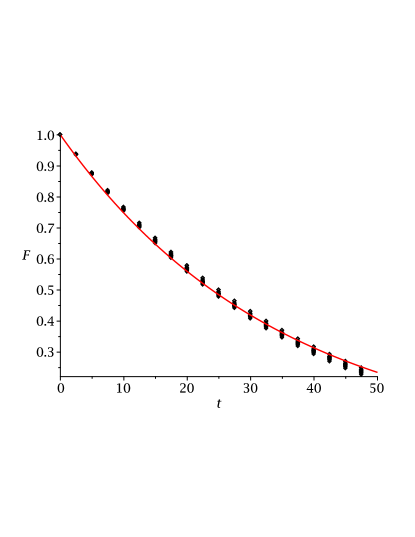
For all $g(t)$ and all parameters $\mu$, the fidelities decay exponentially with decay-rates of approx. 0.029 (For an analysis of the origin of the exponential decay, cf. Ref. Prosen and Znidaric (2002).) Thus, on the level of microscopic quantum states, all modeled scenarios are very similar. The timescale of all sample $g(t)$ is chosen to be comparable to the timescale on which the fidelity decays . Thus, stability of $\langle A(t)\rangle$ cannot be traced back to a stability of the evolution of the quantum state itself, as the latter is always strongly affected by all perturbations.

Now we turn to the dynamics of the expectation value of the observable $A$. ($\langle A(t)\rangle$ and $\langle\tilde{A}(t)\rangle$ denote the expectation values of the observable $A$ for the unperturbed and the perturbated evolution, respectively.) The numerical results are displayed in Fig. 2.

Figure 2: Graphs of the reference expectation value dynamics $g(t)$ (cf. Tab. LABEL:ref_functions, solid lines), the actual quantum dynamics as resulting from the perturbations (symbols), and the dynamics as generated from the heuristic model (14) (dashed lines). There appears to be only one case of full stability: the exponential decay remains unaltered under narrowly banded perturbations, even though all perturbations are equally strong. The agreement of the heuristic model with the actual quantum dynamics is very good.

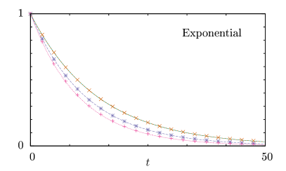
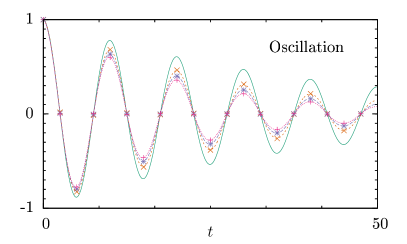
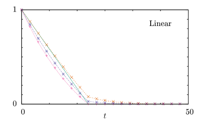
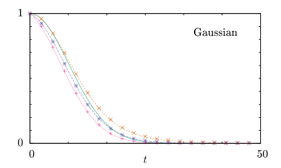
Obviously, in general the perturbations affect $\langle A(t)\rangle$. This influence is moderate due to perturbations being rather weak, but clearly visible and much larger than the statistical effects.

Furthermore the effect of the perturbation does qualitatively depend on the band-width $\mu$: For example the relation $|\langle\tilde{A}(t)\rangle|\leq|\langle A(t)\rangle|$ appears to be always valid for non-banded perturbations ($\mu=2$). If the principle of very slow relaxations always becoming faster upon perturbations was strictly valid, the above relation would always have to hold. It is, however, violated for banded perturbations in some cases. This may be seen nicely at the linear and the Gaussian equilibration.

Among the considered examples there is only one case in which the relaxation dynamics remains entirely unaltered, i.e., is strictly stable: the case of an exponential decay and a narrowly banded perturbation. Note that this holds for all times, also when the fidelity already has decayed substantially. This finding is our first main results. It agrees with the expectations formulated in the context of the examples in Sect. III.

While strict stability only applies to exponential decay and banded perturbations, exponential decay and damped oscillations may be called “quasi-stable” under all perturbations in the following sense: exponential decay and damped oscillations are mapped onto exponential decay and damped oscillations, only the parameters (such as decay constants, etc. change). Such a description does neither apply to the linear nor the Gaussian dynamics.

V Heuristic model of the perturbed dynamics and Memory-Kernel

In the following we present a heuristic model, which describes perturbed dynamics of the previous Sect. rather accurately. This model is based on the notion of a memory kernel. We define the memory-kernel $K(\tau)$, which generates some dynamics $a(t)$, according to the following expression:

$$\derivative{a(t)}{t}=-\int_{0}^{t}K(t-t^{\prime})a(t^{\prime})\mathrm{d}t^{\prime}=-K*a(t)$$ (13)

Often such integro-differential equations of motion are used to calculate the evolution of a variable $a(t)$ from the memory kernel $K(\tau)$. But since Eq. (13) establishes a map $a(t)\Leftrightarrow K(\tau)$ it can also be used the other way round (see Appendix C). To verify our below model (14) numerically, we employ both directions. Expressions like Eq. (13) appear routinely in the context of the Nakajima-Zwanzig projection operator approach, etc. to the expectation values of observables (Nakajima (1958); Zwanzig (1960); Mori (1965)). Metaphorically speaking the memory-kernel describes the way the system remembers its history.

We proceed by describing the original dynamics $a(t):=\langle A(t)\rangle/\langle A(0)\rangle$ as well as the perturbed dynamics $\tilde{a}(t)=\langle\tilde{A}(t)\rangle/\langle\tilde{A}(0)\rangle$ through integro-differential equations of motion of the type (13). The respective memory kernel $K(\tau)$ corresponding to the unperturbed dynamics $a(t)$ may be calculated from $a(t)$, e.g., by means of a Laplace transform, see Appendix C. From this “original” memory kernel $K(\tau)$ we construct a “perturbed” memory kernel $\tilde{K}(\tau)$ as

$$\tilde{K}(\tau)=K(\tau)\exp(-\alpha\tau)-\beta\alpha\delta(\tau).$$ (14)

We find that, for adequate choices of $\alpha,\beta$ the perturbed memory kernel $\tilde{K}(\tau)$ produces almost correctly the respective perturbed dynamics $\tilde{a}(t)$, if inserted into a integro-differential equation of motion of the form (13), i.e., replacing $a(t)\rightarrow\tilde{a}(t)$ and $K(\tau)\rightarrow\tilde{K}(\tau)$ . In (14) $\alpha$ is a non-negative real parameter, which appears to be mainly dependent on the perturbation strength $\epsilon$. $\beta\in[0,1]$ seems to be mainly influenced by the band width of the perturbation $\mu$. The narrow band limit $\mu\rightarrow 0$ corresponds to $\beta=0$, the limit of non-banded perturbations, $\mu\rightarrow 2$ corresponds to $\beta=1$. (For more details on the dependence of $\beta$ on $\mu$, see Appendix. B.) Equations (13,14) represent our heuristic model and our second main result. The remarkable accuracy of this modelling may be captured from Fig. 2, where the dashed lines are calculated from said heuristic model.

For the case of non-banded perturbations ($\beta=1$) it can be shown, that Eq. (14) is equivalent to:

$$\tilde{a}(t)=a(t)\exp(-\alpha t)$$ (15)

Thus, while a non-banded perturbation damps the dynamics of the observable itself, a narrow-banded perturbation damps its memory kernel. The stability and the quasi-stability as found and discussed in the previous Sect. IV are intrinsically built into the model: In general exponential decays and damped oscillations are transformed into exponential decays and a damped oscillation with different decay-constants, oscillation frequencies and phaseshifts, respectively. Moreover, exponential decays are not affected at all by narrowly banded perturbations (small $\beta$).

All our numerical results are in very good agreement with the heuristic model (14) as may be inferred from Fig. 2. The best choice for the parameters $\alpha,\beta$ appears to depend only on $\epsilon,\mu$ but not (or only very weakly) on the original dynamics $g(t)$.

VI Arrow of Time and instability of recurrence dynamics

In this Sect. we come back to the “recurrence dynamics” as discussed in the Introduction, see example given in Eq. (2). We apply our heuristic model (14) to such recurrence dynamics $a_{\mathrm{R}}(t)$, thereby showing that the recurrence gets exponentially damped by both, non-banded and extremely banded perturbations. More concretely we find that

$$\tilde{a}_{\mathrm{R}}(t)\approx a_{\mathrm{R}}(t)\exp(-\alpha t)$$ (16)

holds in both cases. As $\alpha$ appears to depend on the overall perturbation strength $\epsilon$ but not on the bandedness (see text below Eq. (2)), this suggests that banded as well as non-banded perturbations have the very same, strong damping effect on recurrences.

Justifying Eq. (16) for non-banded perturbations is very straight forward as it directly follows from Eq. (15). The case of extremely banded perturbations, i.e., $\mu=0\rightarrow\beta=0$ is more involved. Laplace transformations may be used to find that in this case Eqs. (14, 13) are equivalent to

$$\tilde{a}(t)=a(t)\exp(-\alpha t)+\alpha\int_{0}^{t}\tilde{a}(t^{\prime})a(t-t^{\prime})\exp(-\alpha(t-t^{\prime}))\mathrm{d}t^{\prime}$$ (17)

We now focus on (scaled) expectation value dynamics $a_{\mathrm{R}}(t)$ that first decay within $t\approx\tau^{\prime}$ but feature one recurrence at time $T\gg\tau^{\prime}$ which lasts for $2\tau^{\prime}$ at most, i.e., deviates substantially from 0 only in an interval $T-\tau^{\prime}\leq t\leq T+\tau^{\prime}$. Note that Eq. (2) conforms with this description, however the exponential form of decay and recurrence is not imperative, other forms like Gaussian, linear, etc. are also included in the present consideration. Since $a(t),\tilde{a}(t)$ are both proportional to the respective auto-correlation functions, they are strictly upper bounded by their initial values $a(0)=\tilde{a}(0)=1$, i.e., $|a(t)|\leq 1,|\tilde{a}(t)|\leq 1$.

Thus an upper bound on the convolution-integral in Eq. (17) may be found essentially by replacing $a_{\mathrm{R}}(t),\tilde{a}_{\mathrm{R}}(t)$ by their maxima and restricting the range of integration to the maximum interval on which $a_{\mathrm{R}}(t)$ has non-negligible values:

$$\absolutevalue{\int_{0}^{t}\tilde{a}_{\mathrm{R}}(t^{\prime})a_{\mathrm{R}}(t-t^{\prime})\exp(-\alpha(t-t^{\prime}))\mathrm{d}t^{\prime}}\leq 3\tau^{\prime}$$ (18)

Plugging this back into Eq. (17) unveils that Eq. (16) also holds in the case of extremely banded perturbations up to an additive error of order $\alpha\tau^{\prime}$.

We sum this Sect. up as follows: Even though the above recurrence dynamics may be viewed as being at odds with the arrow of time they are in principle compatible with quantum mechanics. However, the recurrence peak gets damped by generic perturbations. The damping scales exponentially with both, the perturbation strength and the time after which the recurrence occurs. Hence very late recurrences (at large $T$) are very unstable against perturbation, even if the latter are weak.

VII Conclusion and outlook

We studied the influence of (weak) Hamiltonian perturbations on four types of relaxation-dynamics of expectation values. The dynamics have been implemented in high-dimensional, partially random matrix models in accord with the eigenstate thermalization hypothesis. We varied the degree to which the perturbations commute with the observable under consideration and analyzed the effect of this variation on the dynamics. A heuristic model, based on integro-differential equations of motion has been demonstrated to nearly perfectly describe the numerical results. Only exponential decay-dynamics turned out to be stable against perturbations which approximately commute with the respective observable. However, exponential decays and exponentially damped oscillations get mapped onto exponential decays and exponentially damped oscillations by all considered sorts of perturbations. This unique stability of the exponential decay may thus be viewed as a reason for its very frequent occurrence in nature. From the above heuristic model we also concluded that relaxation-dynamics that are at odds with the arrow of time are exponentially unstable. Besides shedding light on such rather fundamental questions of relaxation behavior, there is also a more practical merit: The heuristic model may be used to produce guesses on quantum dynamics under perturbation (if the unperturbed dynamics are known) at numeric costs which are independent of the dimension of the Hilbertspace of the respective system.

Future research may clarify whether the principles found in the paper at hand by means of random matrix models, also apply to concrete physical models, such as spin systems, interacting particle lattice models, etc.

Appendix A Dependence of $\sigma$ on the band-size $\mu$

Here we present a practical scheme for finding $\sigma$ for a given $\mu$. The scheme is accurate to a limit set by the law of large numbers (w.r.t. the dimension $N$). Furthermore we assume semi-circular spectra for the observables $A$.

Starting from Eq. (10), we find:

$$\langle V_{ij}^{2}\rangle= \langle\mathcal{U}^{2}(-1,1)\rangle\sigma^{2}s^{2}(\absolutevalue{a_{i}-a_{j}})$$ (19)

$$= \frac{1}{3}\sigma^{2}s^{2}(\absolutevalue{a_{i}-a_{j}}).$$

Hence the mean squared norm of $V$ may be calculated as follows:

$$\langle||V||_{\mathrm{HS}}^{2}\rangle= \sum\langle V_{ij}^{2}\rangle$$ (20)

$$= \frac{1}{3}\sigma^{2}\sum_{ij}s^{2}(\absolutevalue{a_{i}-a_{j}})$$

$$\approx \frac{1}{3}\sigma^{2}\int_{-1}^{1}\mathrm{d}a_{1}\int_{-1}^{1}\mathrm{d}a_{2}s^{2}(\absolutevalue{a_{1}-a_{2}})\eta(a_{1})\eta(a_{2}),$$

with $\eta(a)=2N/\pi\sqrt{1-a^{2}}$. Thus the last step is based on the assumption of semi-circular spectra. The last step it was used that the spectra of the observables turned out to be approximately semi-circular.

In the same manner the $||H_{0}||_{\mathrm{HS}}$ may be approximated.

$$\langle||H_{0}||_{\mathrm{HS}}^{2}\rangle=\langle\mathcal{U}^{2}(-30,30)\rangle N=300N$$ (21)

Exploiting Eq. (11) yields:

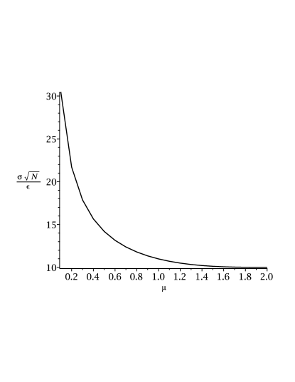
$$\frac{\sigma}{\epsilon}\sqrt{N}\approx 5\pi\left(\int_{-1}^{1}\int_{-1}^{1}s^{2}(\absolutevalue{a_{1}-a_{2}})\eta(a_{1})\eta(a_{2})\mathrm{d}a_{1}\mathrm{d}a_{2}\right)^{-1/2}$$ (22)

Recall that $s(\absolutevalue{a_{1}-a_{2}})$ depends on $\mu$, (10). A graphic representation of Eq. (22) is displayed in Fig. 3.

Figure 3: Dependence of $\sigma$ on the band size $\mu$

Appendix B Determination of parameters $\alpha$ and $\beta$

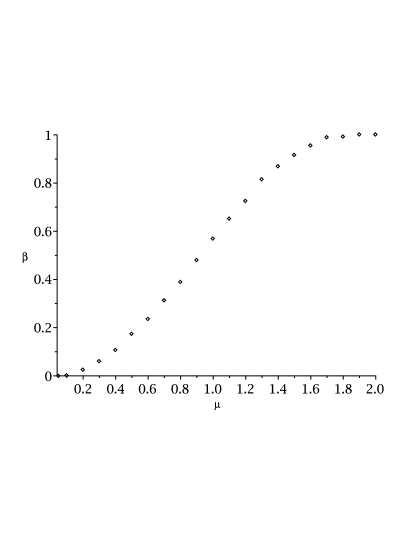
As mentioned in the main text, the parameter $\alpha$ turns out to be almost independent of the band-width $\mu$ of the perturbation matrix. It is, however, controlled by the overall perturbation strength $\epsilon$. Accordingly, the choice $\alpha=0.027$ turns out to be appropriate for all perturbations, regardless of their bandwidth (see Fig. 2). The numerical results indicate that $\beta$ is a function of the band-width $\mu$. To determine this relation, we considered the effect of varying $\mu$ on the exponential decay dynamics. We calculated the dependence of $\beta$ on the band-width $\mu$ by comparing Eq. (14) to the actual perturbed quantum dynamics and by assuming the independence of $\alpha$ on $\mu$, as mentioned above. The result is displayed in Fig. 4

Figure 4: Dependence of the parameter $\beta$ (see. (14)) on the band-size $\mu$ of the perturbation

Appendix C Calculating the Memory-Kernel using Laplace transforms

As stated in the main text (13) establishes an implicit relation between the dynamics $a(t)$ and a memory-kernel $K(\tau)$. This relation can be made explicit by using a Laplace transform. By transforming (13), we find:

$$sA(s)-a(0)=-\kappa(s)A(s)$$ (23)

$A(s)$ and $\kappa(s)$ are the Laplace transforms of $a(t)$ and $K(\tau)$, respectively. By algebraically transforming this equation and applying the inverse Laplace-Transformation, we calculate $K(\tau)$:

$$K(\tau)=\mathcal{L}^{-1}\left\{\frac{a_{0}}{A(s)}-s\right\}$$ (24)