Online Learning Algorithms for
Statistical Arbitrage

1 Introduction

Arbitrage is the risk-free method of making profit from exploiting price differences in different markets. For example, if one stock is trading at a higher price in one market than another, one could buy the stock for the lower price on one market and sell it for the higher price on the other, thereby making profit without taking risks. These pricing disparities have become increasingly hard to capitalize on as they only appear for very short periods of time with the advancements in technology and high-frequency trading. Only those who can recognize and take advantage of arbitrage opportunities first can benefit, turning it into a winner-takes-all situation. This has made it difficult to make consistent profit from price discrepancies, as one needs to recognize them quickly and be the first to leverage them. Yet, arbitrage is a necessary tool in the marketplace as it quickly eliminates market inefficiencies and keeps prices uniform across markets [2, 5, 11, 6, 3, 17].

One type of arbitrage is taking advantage of the difference of the cost of an ETF against the summation of the prices of the stocks in the underlying basket. If the cost of an ETF exceeds the cost of the underlying basket of stocks, then one can buy the individual stocks for the prices on the market, and sell the ETF in order to make a profit.

Another type of arbitrage is through taking advantage of discrepancies within currency conversions, such as in a currency triangle. For example, if one converts a certain currency to another, and then again to another, and then back to the original currency, then the resulting balance does not necessarily equal the initial balance if there exists a discrepancy. Taking advantage of such a discrepancy results in arbitrage.

Another key type of arbitrage is known as statistical arbitrage. Statistical arbitrage relies on historical data and statistics to determine relatively risk-free strategies, although of course this may not always be exactly the case. One simple example of statistical arbitrage is pairs trading. Pairs trading consists of identifying correlations between two or more stocks. When stocks have historically appeared to be strongly correlated, then we can assume that they ultimately will converge when they currently seem to diverge. For example, if stock A and stock B are correlated (they may even be in the same field, such as Coca Cola and Pepsi), and the price of stock A increases while that of stock B remains the same, then we can expect that the two will converge again. In this case, the optimal decision to make is to sell stock A and buy stock B.

This paper deals with algorithms for statistical arbitrage. We present novel techniques for this problem based on online learning. In section 2, we discuss a new formulation of the problem of statistical arbitrage. We present online learning algorithms for statistical arbitrage in Section 3.

2 Problem Formulation

Standard statistical arbitrage algorithms are based on statistic deviations from the mean. However, for non-stationary distributions, which are the typical stochastic processes we observe in the stock market, estimating the mean or the standard deviation is a difficult problem. The problem of learning with non-stationary distributions is an active area of research [9]. Thus, at the heart of these algorithms, there is a key problem, that of non-stationarity. One way to deal with such problems is to use the notion of discrepancy and to design sophisticated time series algorithms such as those proposed by [9]. Alternatively, we can formulate the problem as an instance of online learning which makes no assumption about the distribution. Here, we adopt the latter formulation since it admits the advantage of simplicity while admitting strong regret-based learning guarantees.

3 Algorithm

3.1 Online learning scenario

The standard scenario of online learning can be described as follows: at each round $t\in[1,T]$ the learner receives a point $x_{t}$ out of an input space $X$ and makes a prediction $\hat{y}_{t}\in Y$ for the label of $x_{t}$ out of the output space $Y$. He receives the true label $y_{t}$ and incurs a loss $L(\hat{y}_{t},y_{t})$, where $L\colon Y\times Y\to\mathbb{R}$ is the loss function associated with the problem. No stochastic assumption is made about the input point $x_{t}$ or its label $y_{t}$. The objective of the learner is to minimize its regret, that is the difference between its cumulative loss over $T$ rounds and the loss of the best expert in hindsight.

We want to use online learning to determine when and how much to buy and sell stocks when doing statistical arbitrage. We are going to use the randomized weighted-majority algorithm [10] to help us make decisions in the stock market because it admits a very favorable regret guarantee.

3.2 Randomized weighted majority algorithm

3.2.1 Description

In the randomized scenario of on-line learning, we assume that a set ${\mathscr{A}}=\{1,\ldots,N\}$ of $N$ actions or experts is available. At each round $t\in[T]$, an on-line algorithm ${\mathcal{A}}$ selects a distribution ${\mathbf{p}}_{t}$ over the set of actions, receives a loss vector ${\mathbf{l}}_{t}$, whose $i$th component $l_{t,i}\in[0,1]$ is the loss associated with action $i$, and incurs the expected loss $L_{t}=\sum_{i=1}^{N}p_{t,i}\,l_{t,i}$. The total loss incurred by the algorithm over $T$ rounds is $\mathcal{L}_{T}=\sum_{t=1}^{T}L_{t}$. The total loss associated to action $i$ is $\mathcal{L}_{T,i}=\sum_{t=1}^{T}l_{t,i}$. The minimal loss of a single action is denoted by $\mathcal{L}_{T}^{\min}=\min_{i\in{\mathscr{A}}}\mathcal{L}_{T,i}$. The regret $R_{T}({\mathcal{A}})$ of the algorithm $]{\mathcal{A}}$ after $T$ rounds is then typically defined by the difference of the loss of the algorithm and that of the best single action:

$$R_{T}=\mathcal{L}_{T}-\mathcal{L}_{T}^{\min}.$$

For this presentation of the algorithm, we consider specifically the case of zero-one losses and assume that $l_{t,i}\in\{0,1\}$ for all $t\in[T]$ and $i\in{\mathscr{A}}$.

The Randomized Weighted-Majority algorithm [10] works as follows. The algorithm maintains a distribution $p_{t}$ over a set of $N$ experts. The original distribution $p_{1}$ is initialized to be the uniform distribution. At each round, the loss assigned to each expert is revealed. The algorithm incurs the expected loss over the experts, that is $\sum_{i=1}^{N}p_{t,i}\,l_{t,i}$, and then updates its distribution on the set of experts by multiplying weight $p_{t,i}$ of expert $i$ by $\beta\in(0,1)$ when the expert committed a mistake and leaving it unchanged otherwise. Next, the resulting probability $p_{t+1}$ is obtained after normalization. Figure 1 gives the pseudocode of the algorithm.

 

Randomized-Weighted-Majority $(N)$
991	do
992
993
994	do
995
996	do
997	then
998
999
9910
9911	do
9912
9913

 

Figure 1: Randomized weighted majority algorithm.

Its objective is to minimize its expected regret, that is the difference between its cumulative loss and that of the best expert in hindsight.

3.2.2 Regret Guarantees

The following theorem gives a strong guarantee on the regret $R_{T}$ of the RWM algorithm, showing that it is in $O(\sqrt{T\log N})$. The proof and the presentation are based on [13].

Theorem 3.1

Fix $\beta\in[1/2,1)$. Then, for any $T\geq 1$, the loss of algorithm RWM on any sequence can be bounded as follows:

$$\mathcal{L}_{T}\leq\frac{\log N}{1-\beta}+(2-\beta)\mathcal{L}_{T}^{\min}.$$ (1)

In particular, for $\beta=\max\{1/2,1-\sqrt{(\log N)/T}\}$, the loss can be bounded as:

$$\mathcal{L}_{T}\leq\mathcal{L}_{T}^{\min}+2\sqrt{T\log N}.$$ (2)

Proof

As in many proofs for deriving regret guarantees in on-line learning, we derive upper and lower bounds for the potential function $W_{t}=\sum_{i=1}^{N}w_{t,i}$, $t\in[T]$, and combine these bounds to obtain the result. By definition of the algorithm, for any $t\in[T]$, $W_{t+1}$ can be expressed as follows in terms of $W_{t}$:

$$W_{t+1}=\sum_{i\colon l_{t,i}=0}w_{t,i}+\beta\sum_{i\colon l_{t.i}=1}w_{t,i} =W_{t}+(\beta-1)\sum_{i\colon l_{t,i}=1}w_{t,i}$$

$$=W_{t}+(\beta-1)W_{t}\sum_{i\colon l_{t,i}=1}p_{t,i}$$

$$=W_{t}+(\beta-1)W_{t}L_{t}$$

$$=W_{t}(1-(1-\beta)L_{t}).$$

Thus, since $W_{1}=N$, it follows that $W_{T+1}=N\prod_{t=1}^{T}(1-(1-\beta)L_{t})$. On the other hand, the following lower bound clearly holds: $W_{T+1}\geq\max_{i\in[N]}w_{T+1,i}=\beta^{\mathcal{L}_{T}^{\min}}$. This leads to the following inequality and series of derivations after taking the $\log$ and using the inequalities $\log(1-x)\leq-x$ valid for all $x<1$, and $-\log(1-x)\leq x+x^{2}$ valid for all $x\in[0,1/2]$:

$$\beta^{\mathcal{L}_{T}^{\min}}\leq N\prod_{t=1}^{T}(1-(1-\beta)L_{t})\implies \mathcal{L}_{T}^{\min}\log\beta\leq\log N+\sum_{t=1}^{T}\log(1-(1-\beta)L_{t})$$

$$\implies \mathcal{L}_{T}^{\min}\log\beta\leq\log N-(1-\beta)\sum_{t=1}^{T}L_{t}$$

$$\implies \mathcal{L}_{T}^{\min}\log\beta\leq\log N-(1-\beta)\mathcal{L}_{T}$$

$$\implies \mathcal{L}_{T}\leq\frac{\log N}{1-\beta}-\frac{\log\beta}{1-\beta}\mathcal{L}_{T}^{\min}$$

$$\implies \mathcal{L}_{T}\leq\frac{\log N}{1-\beta}-\frac{\log(1-(1-\beta))}{1-\beta}\mathcal{L}_{T}^{\min}$$

$$\implies \mathcal{L}_{T}\leq\frac{\log N}{1-\beta}+(2-\beta)\mathcal{L}_{T}^{\min}.$$

This shows the first statement. Since $\mathcal{L}_{T}^{\min}\leq T$, this also implies

$$\mathcal{L}_{T}\leq\frac{\log N}{1-\beta}+(1-\beta)T+\mathcal{L}_{T}^{\min}.$$ (3)

Differentiating the upper bound with respect to $\beta$ and setting it to zero gives $\frac{\log N}{(1-\beta)^{2}}-T=0$, that is $\beta=1-\sqrt{(\log N)/T}<1$. Thus, if $1-\sqrt{(\log N)/T}\geq 1/2$, $\beta_{0}=1-\sqrt{(\log N)/T}$ is the minimizing value of $\beta$, otherwise the boundary value $\beta_{0}=1/2$ is the optimal value. The second statement follows by replacing $\beta$ with $\beta_{0}$ in (3). ∎

The bound (2) assumes that the algorithm additionally receives as a parameter the number of rounds $T$. As we shall see in the next section, however, there exists a general doubling trick that can be used to relax this requirement at the price of a small constant factor increase. Inequality 2 can be written directly in terms of the regret $R_{T}$ of the RWM algorithm:

$$R_{T}\leq 2\sqrt{T\log N}.$$ (4)

Thus, for $N$ constant, the regret verifies $R_{T}=O(\sqrt{T})$ and the average regret or regret per round $R_{T}/T$ decreases as $O(1/\sqrt{T})$. These results are known to be optimal.

3.3 Online statistical arbitrage

To use on-line learning algorithms to tackle the problem of statistic arbitrage, we need to specify first the groups of correlated stocks on which to do statistical arbitrage, since we intend to capitalize on deviations the mean. The problem of determining such groups, pairs in the simplest case, is a non-trivial task requiring itself a study of the correlations between stocks over a large period of time. In the following, we will assume that a group of such stocks is already provided to us by specialists of the domain.

Second, we need to specify the set of experts used by our online algorithm. At a high level, the regret analysis of the previous section suggests choosing a relatively large set of experts ($N$) since with the hope that the best expert among them would achieve a small loss in hindsight. Otherwise, our benchmark would be poor and our guarantee rather weak. While a very large $N$ affects the regret guarantee of the RWM algorithm, that effect is rather mild is the dependency on $N$ is only logarithmic.

How should the experts be chosen? One general way of selecting experts is to let existing statistical arbitrage algorithms serve as experts. The regret guarantees then ensure that for large enough $T$, the loss of the online algorithm per round would be very close to that of the best algorithm in hindsight, since $\sqrt{T\log N}/T=\sqrt{\log N/T}\ll 1$ for large $T$.

A widely used class of such algorithms act when the price of a stock crosses a certain factor of the standard deviation from the mean [3, 2]. For example, if the price of a stock increases to a certain positive value of $\gamma$, an expert would suggest selling, while the same expert would suggest buying if the price went below the negative value of $\gamma$. More specifically, these algorithms are based on the $s$-score for each stock which is defined at time $t$ as follows for stock $i$ [2]:

$$s_{i}=\frac{X_{i}(t)-\mu}{\sigma_{i}},$$ (5)

where $X_{i}(t)$ denotes the value of the stock at time $t$, $\mu$ the mean value, and $\sigma_{i}$ the standard deviation. These algorithms then proceed according to the following rules [2]:

$$\begin{cases}\text{Open long position}&\text{if }s_{i}<-1.25\\ \text{Open short position}&\text{if }s_{i}>+1.25\\ \text{Close long position}&\text{if }s_{i}>-0.50\\ \text{Close short position}&\text{if }s_{i}<+0.50.\end{cases}$$ (6)

Thus, these rules determine when to act in statistical arbitrage for different groups of stocks as well as in different time periods.

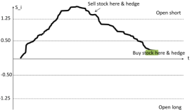
Figure 2: Illustration of some standard statistical arbitrage algorithms.

Instead of the specific values $.5$ and $1.25$ in these rules, we will consider a family of algorithms parameterized by two positive real values $\gamma_{1}$ and $\gamma_{2}$ with $\gamma_{1}<\gamma_{2}$. For $\gamma_{1}=.5$ and $\gamma_{2}=1.25$, the algorithm coincides with the one described above. As suggested by the discussion about the size $N$ of the experts pool, we suggest considering a relatively large set $N$ of pairs $(\gamma_{1},\gamma_{2})$ and therefore experts.

4 Conclusion

We presented a general solution for statistical arbitrage based online learning algorithms and concepts. We gave a full algorithmic and theoretical analysis of the problem within this framework. A key advantage of our algorithm is that it does not require strong stationary assumptions about the stochastic process, which often do not hold in practice. We hope to present preliminary experimental results in support of our algorithms in the future and plan to discuss a number of enhancements, including leveraging online algorithms competing against sequence of experts, which allow for non-static experts to serve as benchmarks in the definition of the regret [8, 7, 1].

References

- Adamskiy et al. [2012] Adamskiy, Dmitry, Koolen, Wouter M, Chernov, Alexey, and Vovk, Vladimir. A closer look at adaptive regret. In ALT, pp. 290–304, 2012.
- Avellaneda [2011] Avellaneda, Marco. Risk and portfolio management: Statisical arbitrage, 2011. URL https://www.math.nyu.edu/faculty/avellane/Lecture8Risk2011.pdf.
- Avellaneda & Lee [2008] Avellaneda, Marco and Lee, Jeong-Hyun. Statistical arbitrage in the u.s. equities market. Technical report, Courant Institute of Mathematical Sciences, 2008.
- Beck & Tetruashvili [2013] Beck, Amir and Tetruashvili, Luba. On the convergence of block coordinate descent type methods. SIAM Journal on Optimization, 23(4):2037–2060, 2013.
- Damghani & Kos [2013] Damghani, Babak Mahdavi and Kos, Andrew. De-arbitraging with a weak smile: Application to skew risks. Wilmott Magazine, pp. 40–49, 2013.
- Fernholz & Cary Maguire [2007] Fernholz, Robert and Cary Maguire, Jr. The statistics of statistical arbitrage. Financial Analysts Journal, pp. 46–52, 2007.
- Hazan & Seshadhri [2009] Hazan, Elad and Seshadhri, Comandur. Efficient learning algorithms for changing environments. In Proceedings of ICML, pp. 393–400. ACM, 2009.
- Herbster & Warmuth [1998] Herbster, Mark and Warmuth, Manfred K. Tracking the best expert. Machine Learning, 32(2):151–178, 1998.
- Kuznetsov & Mohri [2015] Kuznetsov, Vitaly and Mohri, Mehryar. Learning theory and algorithms for forecasting non-stationary time series. In NIPS, 2015.
- Littlestone & Warmuth [1994] Littlestone, Nick and Warmuth, Manfred K. The weighted majority algorithm. Information and Computation, 108(2):212–261, 1994.
- Lo [2010] Lo, Andrew W. Hedge Funds: An Analytic Perspective. Princeton University Press, 2010.
- Luo & Tseng [1992] Luo, Zhi-Quan and Tseng, Paul. On the convergence of the coordinate descent method for convex differentiable minimization. Journal of Optimization Theory and Applications, 72(1):7–35, 1992.
- Mohri et al. [2012] Mohri, Mehryar, Rostamizadeh, Afshin, and Talwalkar, Ameet. Foundations of Machine Learning. Adaptive computation and machine learning. MIT Press, 2012.
- Nesterov [2012] Nesterov, Yurii. Efficiency of coordinate descent methods on huge-scale optimization problems. SIAM Journal on Optimization, 22(2):341–362, 2012.
- Rätsch et al. [2001] Rätsch, Gunnar, Mika, Sebastian, and Warmuth, Manfred K. On the convergence of leveraging. In NIPS, pp. 487–494, 2001.
- Tseng [2001] Tseng, P. Convergence of a block coordinate descent method for nondifferentiable minimization. Journal Optimization Theory and Applications, pp. 475–494, 2001.
- Wu [2007] Wu, Liuren. Statistical arbitrage based on no-arbitrage models, 2007. URL http://faculty.baruch.cuny.edu/lwu/papers/StatArb.pdf.