Structure-preserving numerical integrators for Hodgkin–Huxley-type systems

Abstract.

Motivated by the Hodgkin–Huxley model of neuronal dynamics, we study explicit numerical integrators for “conditionally linear” systems of ordinary differential equations. We show that splitting and composition methods, when applied to the Van der Pol oscillator and to the Hodgkin–Huxley model, do a better job of preserving limit cycles of these systems for large time steps, compared with the “Euler-type” methods (including Euler’s method, exponential Euler, and semi-implicit Euler) commonly used in computational neuroscience, with no increase in computational cost. These limit cycles are important to preserve, due to their role in neuronal spiking. Splitting methods even compare favorably to the explicit exponential midpoint method, which is twice as expensive per step. The second-order Strang splitting method is seen to perform especially well across a range of non-stiff and stiff dynamics.

1. Introduction

This paper is concerned with the numerical integration of conditionally linear systems of ordinary differential equations (ODEs) in $\mathbb{R}^{d}$, which are systems of the form

(1) $$\dot{x}_{i}=a_{i}(x)x_{i}+b_{i}(x),\qquad i=1,\ldots,{d},$$

where $a_{i},b_{i}$ are real-valued functions depending only on $x_{j}$ for $j\neq i$. These systems have the defining property that, if all $x_{j}$ with $j\neq i$ are stationary, then $x_{i}$ satisfies a first-order linear ODE with constant coefficients.

Our motivation comes from neuronal dynamics, where “conditional linearity is a fairly generic property of nonlinear neuronal models” (Mascagni and Sherman [18]). Since these models are nonlinear, computational neuroscientists must use numerical simulation to study the dynamical behavior of individual model neurons, as well as networks of such neurons. We will focus in particular on the model of Hodgkin and Huxley [15], which is one of the most well-known and widely-used biological neuron models.

To simulate (1) as efficiently as possible, one wishes to minimize the number of evaluations of the nonlinear functions $a_{i}$ and $b_{i}$. (This becomes especially important when ${d}$ is large, as is the case for large biological neural networks.) It is therefore desirable to use an explicit numerical integrator that allows for large time step sizes while still producing sufficiently accurate dynamics. One of the main obstacles to doing so is stiffness: when $a_{i}$ is a large negative number, a traditional explicit Runge–Kutta method (like Euler’s method) becomes numerically unstable unless the time step size is very small. For this reason, various authors have proposed using explicit methods designed for stiff systems, such as exponential integrators and semi-implicit integrators; Börgers and Nectow [2] note that such integrators remain stable for much larger time step sizes when simulating Hodgkin–Huxley neurons, on the order of 1 ms, whereas traditional methods require time step sizes on the order of 0.01 ms. They also present numerical evidence that “[a]daptive time-stepping is of questionable use” when simulating networks of neurons [2, Section 7], so the ability to take large time steps is the major arbiter of numerical efficiency.

However, there is another obstacle to taking large time step sizes, having to do with preserving the qualitative dynamics of neuronal spiking in the Hodgkin–Huxley model. When the input current into a neuron is low, the membrane voltage is attracted to a resting equilibrium; however, when the input current exceeds a threshold, the voltage begins rapidly rising and falling periodically. These voltage spikes, called action potentials, are the mechanism by which neurons send signals to one another. From a dynamical systems point of view, this corresponds to a bifurcation: the “resting” fixed point becomes unstable, and the system is attracted to a stable “spiking” limit cycle lying on a two-dimensional center manifold (Hassard [12], Izhikevich [16]). In order to simulate these dynamics faithfully and efficiently, it is therefore desirable that a numerical integrator be able to preserve these limit cycles at large time step sizes. Yet, Euler’s method does a poor job of preserving limit cycles in nonlinear dynamical systems, even for simple systems like the Van der Pol oscillator, unless one takes very small time steps—even smaller than one would need for numerical stability (Hairer and Lubich [8]).

In this paper, we investigate this problem of limit cycle preservation. We show that the exponential Euler and semi-implicit Euler (SI Euler) methods, while superior to the traditional Euler method in terms of stability, have the same fundamental problem of non-preservation of limit cycles. We introduce a new family of splitting and composition methods specifically designed for conditionally linear systems. These methods are just as efficient as the exponential and SI Euler methods, with comparable stability behavior, but they do much better at preserving limit cycles. The splitting methods even compare favorably to the exponential midpoint method proposed by Börgers and Nectow [2], at half the computational cost. These properties are demonstrated both theoretically (using backward error analysis) and numerically for the Van der Pol oscillator, and numerically for the Hodgkin–Huxley model neuron. In particular, a Strang splitting method emerges as the best performer among all the methods considered.

2. Numerical integrators for conditionally linear systems

2.1. Preliminaries

All of the numerical integrators that we consider, old and new, are based on the fact that linear ODEs with constant coefficients can be solved exactly in closed form. That is,

$$\dot{x}=ax+b$$

has the time-$h$ flow given by the explicit formula

$$x(t+h)=\exp(ha)x(t)+\frac{\exp(ha)-1}{ha}hb.$$

Here, $z\mapsto(\exp z-1)/z$ actually means the entire function obtained by removing the singularity at $z=0$, taking $0\mapsto 1$. (This is sometimes called the “relative error exponential” and is implemented in many numerical libraries as exprel.)

In fact, we can also explicitly compute the flow of any Runge–Kutta method applied to this ODE—even an implicit Runge–Kutta method—by replacing the exponential function above with the stability function $z\mapsto r(z)$. For instance, Euler’s method has stability function $r(z)=1+z$, so the time-$h$ flow map taking $x^{n}\mapsto x^{n+1}$ is given by

$$x^{n+1}=(1+ha)x^{n}+hb=x^{n}+h(ax^{n}+b).$$

More interesting is the backward Euler method, with $r(z)=1/(1-z)$; while an implicit method for nonlinear ODEs, in this case it admits the explicit formula

$$x^{n+1}=\frac{1}{1-ha}x^{n}+\frac{1}{1-ha}hb,$$

which rearranges to the more familiar expression,

$$x^{n+1}=x^{n}+h(ax^{n+1}+b).$$

For splitting/composition methods, it can sometimes be desirable to compute an approximate flow, even when the exact flow is computable. For example, the IMEX method for highly-oscillatory problems (Stern and Grinspun [26], McLachlan and Stern [21]) uses the midpoint method instead of the exact flow of a harmonic oscillator, and the Boris method for charged particle dynamics uses the midpoint method instead of the exact flow of the magnetic field (Hairer and Lubich [9, Eq. 1.4]).

As mentioned in the introduction, the defining property of a conditionally linear system (1) is that, if all $x_{j}$ with $j\neq i$ are stationary, then $x_{i}$ satisfies a first-order linear ODE with constant coefficients. We now introduce some notation to help formalize this. Write (1) as $\dot{x}=f(x)$, where $f\colon\mathbb{R}^{d}\rightarrow\mathbb{R}^{d}$ is the vector field with components

$$f_{i}(x)=a_{i}(x)x_{i}+b_{i}(x),\qquad i=1,\ldots,{d}.$$

For $i=1,\ldots,{d}$, let $f^{(i)}\colon\mathbb{R}^{d}\rightarrow\mathbb{R}^{d}$ be the vector field

$$f^{(i)}_{j}(x)=\begin{cases}f_{i}(x),&\text{if }i=j,\\ 0,&\text{if }i\neq j.\end{cases}$$

Let $\varphi^{(i)}_{h}\colon\mathbb{R}^{d}\rightarrow\mathbb{R}^{d}$ denote the exact time-$h$ flow of $f^{(i)}$. Since $f^{(i)}$ holds $x_{j}$ stationary for $j\neq i$, it follows that this flow can be written in closed form as

$$\varphi_{h,j}^{(i)}(x)=\begin{cases}\exp\bigl{(}ha_{i}(x)\bigr{)}x_{i}+\dfrac{\exp\bigl{(}ha_{i}(x)\bigr{)}-1}{ha_{i}(x)}hb_{i}(x),&\text{if }i=j,\\ x_{j},&\text{if }i\neq j.\end{cases}$$

(Here, we use $\varphi^{(i)}_{h,j}$ to denote the $j$th component of $\varphi^{(i)}_{h}$.) Following the discussion above, we might instead approximate $\varphi_{h}^{(i)}$ by an approximate flow $\Phi_{h}^{(i)}$, e.g., by applying a Runge–Kutta method to $f^{(i)}$ with time step size $h$, in which case we would simply replace the exponential function in this formula by the stability function of the method. Note that we may use a different Runge–Kutta method (or the exact flow) for each $i=1,\ldots,{d}$.

We have therefore decomposed the vector field $f$ we wish to integrate as

$$f=f^{(1)}+\cdots+f^{({d})}.$$

Due to conditional linearity, we may integrate each $f^{(i)}$ exactly—or with an arbitrary, possibly-implicit Runge–Kutta method—with only a single evaluation of each of the nonlinear functions $a_{i},b_{i}$. The motivating idea, for all of the methods considered below, is to combine these flows in such a way as to approximate the flow of $f$.

2.2. Euler-type methods

Using the notation established in Section 2.1, we now define a family of “Euler-type” methods for conditionally linear systems. This family includes the classical Euler method, as well as the exponential Euler and SI Euler methods, among others.

Definition .

An Euler-type method for (1) has the form

(2) $$x^{n+1}_{i}=\Phi^{(i)}_{h,i}(x^{n}),\qquad i=1,\ldots,{d},$$

where each $\Phi^{(i)}_{h}$ is either an exact or approximate time-$h$ flow for $f^{(i)}$. More explicitly, this flow has the form

$$x_{i}^{n+1}=r_{i}\bigl{(}ha_{i}(x^{n})\bigr{)}x_{i}^{n}+\dfrac{r_{i}\bigl{(}ha_{i}(x^{n})\bigr{)}-1}{ha_{i}(x^{n})}hb_{i}(x^{n}),\qquad i=1,\ldots,{d},$$

where $r_{i}(z)=1+z+\mathcal{O}(z^{2})$ is either the exponential function or an approximate exponential (e.g., the stability function of a Runge–Kutta method, a Padé approximant, etc.).

The key feature of these methods is that the nonlinear functions $a_{i},b_{i}$ are only evaluated at $x^{n}$ when advancing $x^{n}\mapsto x^{n+1}$. In other words, all of the components are stepped forward in parallel.

Example (Euler’s method).

Suppose $\Phi_{h}^{(i)}$ is Euler’s method applied to $f^{(i)}$ with time step size $h$, for $i=1,\ldots,{d}$. Then (2) becomes

$$x_{i}^{n+1}=x_{i}^{n}+h\bigl{(}a_{i}(x^{n})x_{i}^{n}+b_{i}(x^{n})\bigr{)},\qquad i=1,\ldots,{d},$$

which is just Euler’s method applied to $f$.

Example (exponential Euler method).

Suppose $\Phi_{h}^{(i)}=\varphi_{h}^{(i)}$ is the exact time-$h$ flow of $f^{(i)}$, for $i=1,\ldots,{d}$. Then (2) becomes

$$x_{i}^{n+1}=\exp\bigl{(}ha_{i}(x^{n})\bigr{)}x_{i}^{n}+\dfrac{\exp\bigl{(}ha_{i}(x^{n})\bigr{)}-1}{ha_{i}(x^{n})}hb_{i}(x^{n}),\qquad i=1,\ldots,{d}.$$

This is the exponential Euler method.

Example (SI Euler method).

Suppose $\Phi_{h}^{(i)}$ is the backward Euler method applied to $f^{(i)}$ with time step size $h$, for $i=1,\ldots,{d}$. Then (2) becomes

$$x_{i}^{n+1}=\frac{1}{1-ha_{i}(x^{n})}x^{n}_{i}+\frac{1}{1-ha_{i}(x^{n})}hb_{i}(x^{n}),\qquad i=1,\ldots,{d},$$

which can also be written as

$$x_{i}^{n+1}=x_{i}^{n}+h\bigl{(}a_{i}(x^{n})x_{i}^{n+1}+b_{i}(x^{n})\bigr{)},\qquad i=1,\ldots,{d}.$$

This is the semi-implicit Euler (or SI Euler) method.

All of these methods have order $1$, and all reduce to Euler’s method in the special case that $a_{i}=0$ for all $i=1,\ldots,{d}$.

2.3. The exponential midpoint method

Börgers and Nectow [2] also considered an explicit second-order method, called the exponential midpoint method. Although this is neither an Euler-type nor a splitting/composition method, we include it for comparison.

Definition .

The exponential midpoint method for (1) is

$$x_{i}^{n+1/2} =\exp\bigl{(}\tfrac{1}{2}ha_{i}(x^{n})\bigr{)}x_{i}^{n}+\dfrac{\exp\bigl{(}\tfrac{1}{2}ha_{i}(x^{n})\bigr{)}-1}{\tfrac{1}{2}ha_{i}(x^{n})}\tfrac{1}{2}hb_{i}(x^{n}), \qquad i =1,\ldots,{d}.$$

$$x_{i}^{n+1} =\exp\bigl{(}ha_{i}(x^{n+1/2})\bigr{)}x_{i}^{n}+\dfrac{\exp\bigl{(}ha_{i}(x^{n+1/2})\bigr{)}-1}{ha_{i}(x^{n+1/2})}hb_{i}(x^{n+1/2}), \qquad i =1,\ldots,{d}.$$

The second line is similar to exponential Euler, except $a_{i}$ and $b_{i}$ are evaluated at the approximate midpoint $x^{n+1/2}$, obtained by first taking a half-step of exponential Euler. Note that each nonlinear function is evaluated twice, first at $x^{n}$ and again at $x^{n+1/2}$, so this method is twice as expensive per step as an Euler-type method.

Remark .

This is an example of a two-stage explicit exponential Runge–Kutta method. One may also construct higher-order methods with more intermediate stages (and thus more function evaluations per step). See Hochbruck and Ostermann [14] for a survey of these and other exponential integrators. Also, as before, one may replace the exponential function with an approximate exponential, but we will not consider that generalization here.

2.4. Splitting and composition methods

Before introducing the particular splitting and composition methods that we propose for conditionally linear systems, we briefly review what these classes of methods are, in general. For more on the general theory and application of such methods, we refer the interested reader to the survey by McLachlan and Quispel [20].

A splitting method, for an arbitrary dynamical system $\dot{x}=f(x)$, is based on the idea of decomposing (or “splitting”) the vector field $f$ into a sum of vector fields $f=f^{(1)}+\cdots+f^{(m)}$ and approximating the time-$h$ flow of $f$ by a composition of flows of the $f^{(i)}$. (Here, $f$ need not be conditionally linear, and it might even be a vector field on a manifold.) For example, if $f=f^{(1)}+f^{(2)}$, one might approximate the time-$h$ flow of $f$ by either of

$$\varphi^{(1)}_{h}\circ\varphi^{(2)}_{h},\qquad\varphi^{(2)}_{h/2}\circ\varphi^{(1)}_{h}\circ\varphi^{(2)}_{h/2}.$$

(One may also interchange $\varphi^{(1)}$ and $\varphi^{(2)}$, but we prefer to think of that as corresponding to the alternative splitting of $f$ that interchanges $f^{(1)}$ and $f^{(2)}$.) The first of these, called the Lie–Trotter splitting (Trotter [30]) approximates the flow of $f$ with order $1$; the second, known as the Strang splitting (Strang [28]), approximates it with order $2$. Although it appears that the Strang splitting requires more function evaluations than the Lie–Trotter splitting, note that we may use the semigroup property $\varphi_{h}^{(2)}=\varphi_{h/2}^{(2)}\circ\varphi_{h/2}^{(2)}$ to write

$$(\varphi^{(2)}_{h/2}\circ\varphi^{(1)}_{h}\circ\varphi^{(2)}_{h/2})\circ\cdots\circ(\varphi^{(2)}_{h/2}\circ\varphi^{(1)}_{h}\circ\varphi^{(2)}_{h/2})\\ =\varphi^{(2)}_{h/2}\circ(\varphi_{h}^{(1)}\circ\varphi_{h}^{(2)}\circ\cdots\circ\varphi_{h}^{(2)}\circ\varphi_{h}^{(1)})\circ\varphi^{(2)}_{h/2}.$$

Therefore, with the exception of the first and last step, both methods simply alternate between the flows of $f^{(1)}$ and $f^{(2)}$ and thus have essentially the same computational cost. It is also possible to construct even higher-order splitting methods, by alternating several times between fractional steps of $\varphi^{(1)}$ and $\varphi^{(2)}$, as in the methods of Yoshida [32] and Suzuki [29].

Composition methods are just like splitting methods, except that the flow of $f^{(i)}$ may be replaced by an approximate flow. Unlike exact flows, approximate flows do not generally form a one-parameter group (or semigroup). This motivates the following definitions, which will prepare us to discuss symmetric compositions of approximate flows, analogous to the Strang splitting method.

Definition .

The adjoint of an approximate flow $\Phi_{h}$ is defined to be $\Phi^{\ast}_{h}\coloneqq\Phi_{-h}^{-1}$. We say that $\Phi_{h}$ is symmetric if it is its own adjoint.

Remark .

If a Runge–Kutta method has the stability function $r$, then its adjoint method has the stability function $r^{\ast}(z)=1/r(-z)$.

Here are a few illustrative examples:

• If $\varphi_{h}$ is the exact time-$h$ flow of a vector field, then the group property $\varphi_{h}\circ\varphi_{-h}=\mathrm{id}$ implies that $\varphi_{h}$ is symmetric.

• If $\Phi_{h}$ is Euler’s method, then $\Phi_{h}^{\ast}$ is the backward Euler method. The symmetric methods $\Phi_{h/2}^{\ast}\circ\Phi_{h/2}$ and $\Phi_{h/2}\circ\Phi_{h/2}^{\ast}$ are the trapezoid and midpoint methods, respectively.

• If $\Phi_{h}=\varphi_{h}^{(1)}\circ\varphi^{(2)}_{h}$ is the Lie–Trotter splitting method, then $\Phi_{h}^{\ast}=\varphi_{h}^{(2)}\circ\varphi^{(1)}_{h}$ is the Lie–Trotter method for the splitting with $f^{(1)}$ and $f^{(2)}$ interchanged. The symmetric methods $\Phi_{h/2}^{\ast}\circ\Phi_{h/2}$ and $\Phi_{h/2}\circ\Phi_{h/2}^{\ast}$ are the Strang splitting methods for the original splitting and for the splitting with $f^{(1)}$ and $f^{(2)}$ interchanged, respectively.

For instance, given a splitting $f=f^{(1)}+f^{(2)}$, we may consider the composition methods

$$\Phi_{h}^{(1)}\circ\Phi_{h}^{(2)},\qquad\Phi_{h/2}^{(2)\ast}\circ\Phi_{h/2}^{(1)\ast}\circ\Phi_{h/2}^{(1)}\circ\Phi_{h/2}^{(2)},$$

which are the composition-method generalizations of the Lie–Trotter and Strang splitting methods, respectively. (We recover precisely these splitting methods in the special case where we take $\Phi^{(1)}=\varphi^{(1)}$ and $\Phi^{(2)}=\varphi^{(2)}$ to be the exact flows.) In particular, the first composition method has order $1$, while the second is symmetric and has order $2$. As with splitting methods, one may construct higher-order (symmetric) composition methods by alternating several fractional steps of these approximate flows (McLachlan [19]).

Before returning to conditionally linear systems, we finally note that for $f=f^{(1)}+\cdots+f^{(m)}$ with arbitrary $m$, we may generalize the Lie–Trotter and Strang splitting and composition methods above by the following:

$$\Phi_{h}^{(1)}\circ\cdots\circ\Phi_{h}^{(m)},\qquad\Phi_{h/2}^{(m)\ast}\circ\cdots\circ\Phi_{h/2}^{(1)\ast}\circ\Phi_{h/2}^{(1)}\circ\cdots\circ\Phi_{h/2}^{(m)}.$$

Again, the first of these has order $1$, while the second is symmetric and has order $2$. For more on these splitting and composition methods and their higher-order generalizations, we again refer the reader to the survey by McLachlan and Quispel [20].

Definition .

Given a conditionally linear system (1), we consider both the non-symmetric composition method

$$x^{n+1}=(\Phi_{h}^{(1)}\circ\cdots\circ\Phi_{h}^{({d})})(x^{n}),$$

and the symmetric composition method

$$x^{n+1}=(\Phi_{h/2}^{({d})\ast}\circ\cdots\circ\Phi_{h/2}^{(1)\ast}\circ\Phi_{h/2}^{(1)}\circ\cdots\circ\Phi_{h/2}^{({d})})(x^{n}),$$

where each $\Phi_{h}^{(i)}$ is either an exact or approximate time-$h$ flow for $f^{(i)}$. We call these splitting methods when all of the $\Phi_{h}^{(i)}$ are exact flows.

Remark .

As with Euler-type methods, each flow $\Phi_{h}^{(i)}$ is defined by $r_{i}(z)=1+z+\mathcal{O}(z^{2})$, which is an exact or approximate exponential. As in Section 2.4, its adjoint $\Phi_{h}^{(i)\ast}$ corresponds to $r_{i}^{\ast}(z)=1/r_{i}(-z)$.

Remark .

In the special case where the flows $\Phi_{h}^{(1)},\ldots,\Phi_{h}^{({d})}$ commute, the non-symmetric splitting method is identical to the corresponding Euler-type method. (This is true, for instance, if $a_{i},b_{i}$ are constants.) In this case, the symmetric splitting method is similarly identical to the Euler-type method $\Phi_{h,i}=(\Phi_{h/2}^{(i)\ast}\circ\Phi_{h/2}^{(i)})_{i}$.

We now give examples of these methods in the ${d}=2$ case, i.e.,

$$\dot{x}_{1} =a_{1}(x_{2})x_{1}+b_{1}(x_{2}),$$

$$\dot{x}_{2} =a_{2}(x_{1})x_{2}+b_{2}(x_{1}).$$

Here, we have made explicit in the notation that $a_{1},b_{1}$ depend only on $x_{2}$ and $a_{2},b_{2}$ depend only on $x_{1}$.

Example (symplectic Euler and Störmer/Verlet methods).

Suppose we take $\Phi_{h}^{(1)}$ to be the time-$h$ flow of Euler’s method and $\Phi_{h}^{(2)}$ to be the time-$h$ flow of the backward Euler method.

The non-symmetric composition method can be written as the algorithm

$$x_{2}^{n+1} =x_{2}^{n}+h\bigl{(}a_{2}(x_{1}^{n})x_{2}^{n+1}+b_{2}(x_{1}^{n})\bigr{)},$$

$$x_{1}^{n+1} =x_{1}^{n}+h\bigl{(}a_{1}(x_{2}^{n+1})x_{1}^{n}+b_{1}(x_{2}^{n+1})\bigr{)}.$$

This is an order-$1$ partitioned Runge–Kutta method known as the symplectic Euler method (since its flow is symplectic when applied to Hamiltonian systems). Note that this is actually an explicit method, since the first step only requires solving a linear equation for $x_{2}^{n+1}$, as with the SI Euler method.

The symmetric composition method can be written as the algorithm

$$x_{2}^{n+1/2} =x_{2}^{n}+\frac{1}{2}h\bigl{(}a_{2}(x_{1}^{n})x_{2}^{n+1/2}+b_{2}(x_{1}^{n})\bigr{)},$$

$$x_{1}^{n+1/2} =x_{1}^{n}+\frac{1}{2}h\bigl{(}a_{1}(x_{2}^{n+1/2})x_{1}^{n}+b_{1}(x_{2}^{n+1/2})\bigr{)},$$

$$x_{1}^{n+1} =x_{1}^{n+1/2}+\frac{1}{2}h\bigl{(}a_{1}(x_{2}^{n+1/2})x_{1}^{n+1}+b_{1}(x_{2}^{n+1/2})\bigr{)},$$

$$x_{2}^{n+1} =x_{2}^{n+1/2}+\frac{1}{2}h\bigl{(}a_{2}(x_{1}^{n+1})x_{2}^{n+1/2}+b_{2}(x_{1}^{n+1})\bigr{)}.$$

Note that the second and third steps can be combined, yielding

$$x_{2}^{n+1/2} =x_{2}^{n}+\frac{1}{2}h\bigl{(}a_{2}(x_{1}^{n})x_{2}^{n+1/2}+b_{2}(x_{1}^{n})\bigr{)},$$

$$x_{1}^{n+1} =x_{1}^{n}+h\biggl{(}a_{1}(x_{2}^{n+1/2})\frac{x_{1}^{n}+x_{1}^{n+1}}{2}+b_{1}(x_{2}^{n+1/2})\biggr{)},$$

$$x_{2}^{n+1} =x_{2}^{n+1/2}+\frac{1}{2}h\bigl{(}a_{2}(x_{1}^{n+1})x_{2}^{n+1/2}+b_{2}(x_{1}^{n+1})\bigr{)},$$

i.e., we use the fact that $\Phi_{h/2}^{(1)\ast}\circ\Phi_{h/2}^{(1)}$ is the time-$h$ flow of the trapezoid method for $f^{(1)}$. This is an order-$2$ symplectic partitioned Runge–Kutta method known as the Störmer/Verlet (or leapfrog) method. As with the non-symmetric composition, this is actually an explicit method, since we need only solve linear equations for $x_{2}^{n+1/2}$ and $x_{1}^{n+1}$.

Example (splitting methods).

Suppose we take $\Phi_{h}^{(1)}=\varphi_{h}^{(1)}$ and $\Phi_{h}^{(2)}=\varphi_{h}^{(2)}$ to be the exact time-$h$ flows of $f^{(1)}$ and $f^{(2)}$, respectively.

The non-symmetric splitting method is

$$x_{2}^{n+1} =\exp\bigl{(}ha_{2}(x_{1}^{n})\bigr{)}x_{2}^{n}+\dfrac{\exp\bigl{(}ha_{2}(x_{1}^{n})\bigr{)}-1}{ha_{2}(x_{1}^{n})}hb_{2}(x_{1}^{n}),$$

$$x_{1}^{n+1} =\exp\bigl{(}ha_{1}(x_{2}^{n+1})\bigr{)}x_{1}^{n}+\dfrac{\exp\bigl{(}ha_{1}(x_{2}^{n+1})\bigr{)}-1}{ha_{1}(x_{2}^{n+1})}hb_{1}(x_{2}^{n+1}),$$

and the symmetric splitting method is

$$x_{2}^{n+1/2} =\exp\bigl{(}\tfrac{1}{2}ha_{2}(x_{1}^{n})\bigr{)}x_{2}^{n}+\dfrac{\exp\bigl{(}\tfrac{1}{2}ha_{2}(x_{1}^{n})\bigr{)}-1}{\tfrac{1}{2}ha_{2}(x_{1}^{n})}\tfrac{1}{2}hb_{2}(x_{1}^{n}),$$

$$x_{1}^{n+1} =\exp\bigl{(}ha_{1}(x_{2}^{n+1/2})\bigr{)}x_{1}^{n}+\dfrac{\exp\bigl{(}ha_{1}(x_{2}^{n+1/2})\bigr{)}-1}{ha_{1}(x_{2}^{n+1/2})}hb_{1}(x_{2}^{n+1/2}),$$

$$x_{2}^{n+1} =\exp\bigl{(}\tfrac{1}{2}ha_{2}(x_{1}^{n+1})\bigr{)}x_{2}^{n+1/2}+\dfrac{\exp\bigl{(}\tfrac{1}{2}ha_{2}(x_{1}^{n+1})\bigr{)}-1}{\tfrac{1}{2}ha_{2}(x_{1}^{n+1})}\tfrac{1}{2}hb_{2}(x_{1}^{n+1}).$$

As previously stated, the non-symmetric splitting method has order $1$, whereas the symmetric splitting method has order $2$.

Note that all of the non-symmetric methods (and all of the symmetric methods) agree in the special case where $a_{i}=0$ for $i=1,\ldots,{d}$. For example, when ${d}=2$ and $a_{1}=a_{2}=0$, the non-symmetric methods all reduce to symplectic Euler, while the symmetric methods all reduce to Störmer/Verlet.

2.5. Combining Euler-type and splitting/composition methods

We briefly discuss a generalization that includes both Euler-type and splitting/composition methods, as well as methods combining aspects of each. The idea is to partition the components $\{1,\ldots,{d}\}$ and to apply an Euler-type method across partitions while using a splitting/composition method within each partition. We will not analyze these generalized methods in this paper, but we mention them due to their parallel-implementation advantages when ${d}$ is large.

Let $0=i_{0}<\cdots<i_{k}={d}$, where each $i_{j}$ is an integer. This partitions $\{1,\ldots,{d}\}$ into the $k$ subsets $\{i_{j-1}+1,\ldots,i_{j}\}$. We may then consider the non-symmetric method

$$\Phi_{h,i}=(\Phi_{h}^{(i_{j-1}+1)}\circ\cdots\circ\Phi_{h}^{(i_{j})})_{i},\qquad i=i_{j-1}+1,\ldots,i_{j},\quad j=1,\ldots,k.$$

This is an Euler-type method in the special case when we partition into ${d}$ subsets of size $1$, and it is a non-symmetric composition method when we partition into $1$ subset of size ${d}$. Likewise, we may consider

$$\Phi_{h,i}=(\Phi_{h/2}^{(i_{j})\ast}\circ\cdots\circ\Phi_{h/2}^{(i_{j-1}+1)\ast}\circ\Phi_{h/2}^{(i_{j-1}+1)}\circ\cdots\circ\Phi_{h/2}^{(i_{j})})_{i},\\ i=i_{j-1}+1,\ldots,i_{j},\quad j=1,\ldots,k,$$

which is (respectively) an Euler-type method or a symmetric composition method in the two special cases mentioned above.

While splitting and composition methods have desirable structure-preserving properties (as we will see in the subsequent sections), one disadvantage, compared to Euler-type methods, is that the flows must be evaluated in series rather than in parallel. When ${d}$ is large, it may be computationally infeasible to do this. The generalization above is a compromise that allows one to partition each step into $k$ pieces that may be computed in parallel. For example, one might simulate a network of $k$ Hodgkin–Huxley neurons in this way.

3. Limit cycle preservation for the Van der Pol oscillator

3.1. The Van der Pol oscillator

The simple harmonic oscillator is a Hamiltonian system with $H(x_{1},x_{2})=\frac{1}{2}(x_{1}^{2}+x_{2}^{2})$, so that

$$\dot{x}_{1} =\hphantom{-}\frac{\partial H}{\partial x_{2}} =\hphantom{-}x_{2},$$

$$\dot{x}_{2} =-\frac{\partial H}{\partial x_{1}} =-x_{1}.$$

The Van der Pol oscillator is the conditionally linear system

(3) $$\dot{x}_{1} =x_{2},$$

$$\dot{x}_{2} =\epsilon(1-x_{1}^{2})x_{2}-x_{1},$$

which adds a nonlinear dissipation term proportional to the constant parameter $\epsilon$ (van der Pol [31]). Due to its dynamical similarities with the more complex Hodgkin–Huxley model, the Van der Pol oscillator has played an important role in simplified models of neuronal spiking: specifically, it is the foundation for the Fitzhugh–Nagumo model [7, 24, 16], of which it is a special case.

We begin by discussing the non-stiff case, when $\epsilon\ll 1$. If we transform into the “action-angle” coordinates $(a,\theta)$, defined by $x_{1}=\sqrt{2a}\cos\theta$, $x_{2}=\sqrt{2a}\sin\theta$, then (3) becomes

$$\dot{a} =\epsilon(1-2a\cos^{2}\theta)2a\sin^{2}\theta,$$

$$\dot{\theta} =-1+\epsilon(1-2a\cos^{2}\theta)\cos\theta\sin\theta.$$

When $\epsilon\ll 1$, we have $\dot{\theta}\approx-1$. Since $a$ evolves much more slowly, one may obtain approximate dynamics by averaging over $\theta\in\mathbb{T}\coloneqq\mathbb{R}/2\pi\mathbb{Z}$, i.e., over one period of oscillation. Observe that $\sin^{2}\theta$ and $4\cos^{2}\theta\sin^{2}\theta=\sin^{2}(2\theta)$ both have average $\frac{1}{2}$, so the averaged dynamics are given by

$$\dot{a}\approx\epsilon(a-\tfrac{1}{2}a^{2})=\epsilon a(1-\tfrac{1}{2}a).$$

This has fixed points $a=0,2$. When $\epsilon<0$, the fixed point at $a=0$ is stable and the one at $a=2$ is unstable, whereas when $\epsilon>0$, the fixed point at $a=0$ is unstable and the one at $a=2$ is stable. In the $(x_{1},x_{2})$-plane, these equilibria correspond to a fixed point at the origin and a limit cycle given by the circle with radius $2$ centered at the origin, and the bifurcation at $\epsilon=0$ is a Hopf bifurcation.

The stiff case, when $\epsilon\gg 1$, is most easily understood after performing the change of variables $y_{1}=x_{1}$, $y_{2}=x_{1}-x_{1}^{3}/3-x_{2}/\epsilon$, known as the Liénard transformation [17]. The system (3) then becomes

$$\dot{y}_{1} =\epsilon(y_{1}-y_{1}^{3}/3-y_{2}),$$

$$\dot{y}_{2} =-y_{1}/\epsilon.$$

The $y_{1}$-nullcline (i.e., where $\dot{y}_{1}=0$) is given by the cubic $y_{2}=y_{1}-y_{1}^{3}/3$. Since $y_{1}$ evolves much more quickly than $y_{2}$, solutions are quickly attracted to the cubic nullcline. They then move slowly along the nullcline until they reach an extremum, at which point they fall off the nullcline and quickly jump horizontally to the other branch of the nullcline. This repeats periodically, describing the attractive limit cycle of the stiff Van der Pol oscillator.

Reference solutions for the Van der Pol oscillator, in both the non-stiff and stiff cases, are shown in Figure 1.

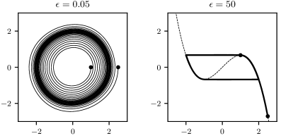
Figure 1. Reference solutions for the Van der Pol oscillator. Left: When $0<\epsilon\ll 1$, solutions are attracted to a limit cycle with approximate radius $2$ in the $(x_{1},x_{2})$-plane. Right: When $\epsilon\gg 1$, the attractive limit cycle jumps between branches of the cubic nullcline (dashed line) in the $(y_{1},y_{2})$-plane, given by the Liénard transformation $(y_{1},y_{2})=(x_{1},x_{1}-x_{1}^{3}/3-x_{2}/\epsilon)$.

3.2. Limit cycle behavior of numerical methods (non-stiff case)

We now analyze the limit cycle behavior of Euler-type methods, the exponential midpoint method, and splitting/composition methods for the Van der Pol oscillator in the non-stiff case $\epsilon\ll 1$. Following the approach of Hairer and Lubich [8] (see also Hairer et al. [10, Chapter XII]), we do so using backward error analysis. That is, we view a numerical method for the vector field $f$ as formally the flow of a modified vector field $\widetilde{f}=f+hf^{[1]}+h^{2}f^{[2]}+\cdots$. This modified vector field is calculated by writing the numerical method as $x^{n+1}=\widetilde{x}(t^{n}+h)$, where $\widetilde{x}$ formally solves the initial value problem $\dot{\widetilde{x}}=\widetilde{f}(\widetilde{x})$, $\widetilde{x}(t^{n})=x^{n}$, and matching terms in the Taylor expansion.

Remark .

By “formally,” we mean that $\widetilde{x}$ and $\widetilde{f}$ are formal power series, which may diverge. However, this formal procedure may be interpreted rigorously by truncating the asymptotic expansions and proving suitable error estimates; see Hairer et al. [10, Chapter IX].

3.2.1. Euler-type methods

Euler’s method for the Van der Pol oscillator (3) is

$$x_{1}^{n+1} =x_{1}^{n}+hx_{2}^{n},$$

$$x_{2}^{n+1} =x_{2}^{n}+h\Bigl{(}\epsilon\bigl{(}1-(x_{1}^{n})^{2}\bigr{)}x_{2}^{n}-x_{1}^{n}\Bigr{)}.$$

To calculate the modified vector field $\widetilde{f}$, we write the modified system

$$\dot{\widetilde{x}}_{1} =\widetilde{x}_{2}+hf_{1}^{[1]}(\widetilde{x})+\mathcal{O}(h^{2}),$$

$$\dot{\widetilde{x}}_{2} =\epsilon(1-\widetilde{x}_{1}^{2})\widetilde{x}_{2}-\widetilde{x}_{1}+hf^{[1]}_{2}(\widetilde{x})+\mathcal{O}(h^{2}).$$

Taylor expanding the first component gives

$$\widetilde{x}_{1}(t^{n}+h) =\widetilde{x}_{1}(t_{n})+h\dot{\widetilde{x}}_{1}(t_{n})+\frac{1}{2}h^{2}\ddot{\widetilde{x}}_{1}(t_{n})+\mathcal{O}(h^{3})$$

$$=x_{1}^{n}+h\widetilde{x}_{2}+h^{2}\Bigl{(}f_{1}^{[1]}(x^{n})-\frac{1}{2}x_{1}^{n}+\mathcal{O}(\epsilon)\Bigr{)}+\mathcal{O}(h^{3}).$$

Likewise, for the second component,

$$\widetilde{x}_{2}(t^{n}+h)=x_{2}^{n}+h\Bigl{(}\epsilon\bigl{(}1-(x_{1}^{n})^{2}\bigr{)}x_{2}^{n}-x_{1}^{n}\Bigr{)}+h^{2}\Bigl{(}f_{2}^{[1]}(x^{n})-\frac{1}{2}x_{2}^{n}+\mathcal{O}(\epsilon)\Bigr{)}+\mathcal{O}(h^{3}).$$

Matching terms with the expressions for $x^{n+1}$ implies $f_{1}^{[1]}(\widetilde{x})=\frac{1}{2}\widetilde{x}_{1}+\mathcal{O}(\epsilon)$ and $f_{2}^{[1]}(\widetilde{x})=\frac{1}{2}\widetilde{x}_{2}+\mathcal{O}(\epsilon)$, so Euler’s method is formally the flow of the modified system

(4) $$\dot{\widetilde{x}}_{1} =\widetilde{x}_{2}+\frac{1}{2}h\widetilde{x}_{1}+\mathcal{O}(h^{2}+\epsilon h),$$

$$\dot{\widetilde{x}}_{2} =\epsilon(1-\widetilde{x}_{1}^{2})\widetilde{x}_{2}-\widetilde{x}_{1}+\frac{1}{2}h\widetilde{x}_{2}+\mathcal{O}(h^{2}+\epsilon h).$$

Transforming into action-angle coordinates and averaging over one period of oscillation, as in Section 3.1, gives

$$\dot{\widetilde{a}} \approx\epsilon(\widetilde{a}-\tfrac{1}{2}\widetilde{a}^{2})+h\widetilde{a}+\mathcal{O}(h^{2}+\epsilon h)$$

$$=\epsilon\widetilde{a}(1+\tfrac{h}{\epsilon}-\tfrac{1}{2}\widetilde{a})+\mathcal{O}(h^{2}+\epsilon h).$$

This has an equilibrium at $\widetilde{a}=2(1+h/\epsilon)$, so the corresponding limit cycle in the $(\widetilde{x}_{1},\widetilde{x}_{2})$-plane is a circle of radius $2\sqrt{1+h/\epsilon}$ centered at the origin. This gives a poor approximation of the true limit cycle, which has radius $2$, unless $h\ll\epsilon$. As noted in Section 1, this step size requirement is even more restrictive than that needed for numerical stability. The foregoing argument appears in Hairer and Lubich [8] and in Hairer et al. [10, Chapter XII].

We next show that all Euler-type methods, including the exponential Euler and SI Euler methods, share this poor limit cycle behavior.

Proposition .

For any Euler-type method applied to the Van der Pol oscillator, the modified vector field is given by (4). Consequently, numerical solutions have a limit cycle with approximate radius $2\sqrt{1+h/\epsilon}$ for $\epsilon\ll 1$.

Proof.

Since $a_{1}=0$, the first component of any Euler-type method agrees with Euler’s method, i.e.,

$$x_{1}^{n+1}=x_{1}^{n}+hx_{2}^{n}.$$

For the second component, using $r_{2}(z)=1+z+\mathcal{O}(z^{2})$ and $\bigl{(}r_{2}(z)-1\bigr{)}/z=1+\mathcal{O}(z)$, we have

$$x_{2}^{n+1} =\Bigl{(}1+h\epsilon\bigl{(}1-(x_{1}^{n})^{2}\bigr{)}+\mathcal{O}(\epsilon^{2}h^{2})\Bigr{)}x_{2}^{n}-h\bigl{(}1+\mathcal{O}(\epsilon h)\bigr{)}x_{1}^{n}$$

$$=x_{2}^{n}+h\Bigl{(}\epsilon\bigl{(}1-(x_{1}^{n})^{2}\bigr{)}x_{2}^{n}-x_{1}^{n}\Bigr{)}+\mathcal{O}(\epsilon h^{2}).$$

Hence, $f^{[1]}$ for an Euler-type method only differs from that for Euler’s method by $\mathcal{O}(\epsilon)$, which becomes $\mathcal{O}(\epsilon h)$ in the modified vector field. However, this is just absorbed by the error term in (4). ∎

3.2.2. The exponential midpoint method

As with the Euler-type methods, we may also use backward error analysis to analyze the limit cycle behavior of the exponential midpoint method. Since the method is second-order, the first-order term $f^{[1]}$ in the modified vector field vanishes, and we have

$$\dot{\widetilde{x}}_{1} =\widetilde{x}_{2}+h^{2}f_{1}^{[2]}(\widetilde{x})+\mathcal{O}(h^{3}),$$

$$\dot{\widetilde{x}}_{2} =\epsilon(1-\widetilde{x}_{1}^{2})\widetilde{x}_{2}-\widetilde{x}_{1}+h^{2}f^{[2]}_{2}(\widetilde{x})+\mathcal{O}(h^{3}).$$

Naïvely, one would expect these $\mathcal{O}(h^{2})$ errors to result in an $\mathcal{O}(h^{2}/\epsilon)$ error in the limit cycle radius. However, Taylor expanding and matching terms yields, after a calculation,

$$\dot{\widetilde{x}}_{1} =\widetilde{x}_{2}+\frac{1}{6}h^{2}\widetilde{x}_{2}+\mathcal{O}(h^{3}+\epsilon h^{2}),$$

$$\dot{\widetilde{x}}_{2} =\epsilon(1-\widetilde{x}_{1}^{2})\widetilde{x}_{2}-\widetilde{x}_{1}-\frac{1}{6}h^{2}\widetilde{x}_{1}+\mathcal{O}(h^{3}+\epsilon h^{2}),$$

so these $h^{2}$ terms actually cancel in $\dot{\widetilde{a}}=\widetilde{x}_{1}\dot{\widetilde{x}}_{1}+\widetilde{x}_{2}\dot{\widetilde{x}}_{2}$. Therefore, we need to compute out to $f^{[3]}$ to obtain the leading-order error term for the limit cycle radius.

Proposition .

For the exponential midpoint method applied to the Van der Pol oscillator, numerical solutions have a limit cycle with approximate radius $2\sqrt{1+h^{3}/(4\epsilon)}$ for $\epsilon\ll 1$.

Proof.

Taylor expanding and matching terms to compute $f^{[3]}$ gives

$$\dot{\widetilde{x}}_{1} =\widetilde{x}_{2}+\frac{1}{6}h^{2}\widetilde{x}_{2}+\frac{1}{8}h^{3}\widetilde{x}_{1}+\mathcal{O}(h^{4}+\epsilon h^{2}),$$

$$\dot{\widetilde{x}}_{2} =\epsilon(1-\widetilde{x}_{1}^{2})\widetilde{x}_{2}-\widetilde{x}_{1}-\frac{1}{6}h^{2}\widetilde{x}_{1}+\frac{1}{8}h^{3}\widetilde{x}_{2}+\mathcal{O}(h^{4}+\epsilon h^{2}),$$

Transforming into action-angle coordinates, the $h^{2}$ terms cancel in $\dot{\widetilde{a}}=\widetilde{x}_{1}\dot{\widetilde{x}}_{1}+\widetilde{x}_{2}\dot{\widetilde{x}}_{2}$, as noted above, while the $h^{3}$ terms become $\frac{1}{8}h^{3}(\widetilde{x}_{1}^{2}+\widetilde{x}_{2}^{2})=\frac{1}{4}h^{3}\widetilde{a}$. Therefore, averaging over one period of oscillation gives

$$\dot{\widetilde{a}}\approx\epsilon\widetilde{a}(1-\tfrac{1}{2}\widetilde{a})+\tfrac{1}{4}h^{3}\widetilde{a}=\epsilon\widetilde{a}(1+\tfrac{h^{3}}{4\epsilon}-\tfrac{1}{2}\widetilde{a}),$$

which has an equilibrium at $\widetilde{a}=2\bigl{(}1+h^{3}/(4\epsilon)\bigr{)}$. The corresponding limit cycle in the $(\widetilde{x}_{1},\widetilde{x}_{2})$-plane is a circle of radius $2\sqrt{1+h^{3}/(4\epsilon)}$ centered at the origin. ∎

It follows that, in order to obtain a good approximation of the limit cycle using the exponential midpoint method, we require $h^{3}\ll\epsilon$. This allows for larger time steps than Euler-type methods, which require $h\ll\epsilon$, but still we cannot choose $h$ independently of $\epsilon$.

3.2.3. Splitting and composition methods

We next examine the limit cycle behavior of splitting and composition methods for the Van der Pol oscillator. Instead of explicitly computing the modified vector field, we exploit the fact that the modified vector field is Hamiltonian when $\epsilon=0$. This is an application of a general argument for perturbed Hamiltonian systems due to Stoffer [27], Hairer and Lubich [8]. We remark that those authors were primarily considering symplectic integrators, such as symplectic (partitioned) Runge–Kutta methods, which are symplectic when applied to any Hamiltonian system. Although the splitting and composition methods we consider are not symplectic in this more general sense—they are generally non-symplectic for non-separable Hamiltonian systems—the argument only requires that the modified vector field be Hamiltonian when $\epsilon=0$, which it is in this case.

When $\epsilon=0$, the Van der Pol oscillator reduces to the simple harmonic oscillator. In this case, the splitting $f=f^{(1)}+f^{(2)}$ corresponds to the Hamiltonian splitting $H=H^{(1)}+H^{(2)}$, i.e., $f^{(i)}$ is the Hamiltonian vector field for $H^{(i)}(x)=\frac{1}{2}x_{i}^{2}$. Since $a_{i}=0$, any approximate flow $\Phi_{h}^{(i)}$ coincides with the exact flow $\varphi_{h}^{(i)}$, so for the simple harmonic oscillator, every composition method is just a splitting method.

Since vector fields form a Lie algebra with the Jacobi–Lie bracket, the modified vector field $\widetilde{f}$ for the non-symmetric splitting method $\varphi_{h}^{(1)}\circ\varphi_{h}^{(2)}$ may be computed by applying the Baker–Campbell–Hausdorff formula to the vector fields $f^{(1)},f^{(2)}$. Moreover, since Hamiltonian vector fields are closed with respect to the Jacobi–Lie bracket (i.e., they form a Lie subalgebra), $\widetilde{f}=f+hf^{[1]}+\cdots$ is formally the Hamiltonian vector field of a modified Hamiltonian $\widetilde{H}=H+hH^{[1]}+\cdots$. In fact, the modified Hamiltonian can itself be computed using the Baker–Campbell–Hausdorff formula, by applying it to $H^{(1)},H^{(2)}$ with the Poisson bracket; this works because the Lie algebra of Hamiltonian vector fields with the Jacobi–Lie bracket is isomorphic to that of Hamiltonian functions with the Poisson bracket.

This approach is due to Yoshida [33], and it may be generalized to show that any Hamiltonian splitting method, including symmetric and higher-order splittings, has a modified vector field that is again Hamiltonian. Moreover, when the splitting method has order $p$, we have $\widetilde{f}=f+\mathcal{O}(h^{p})$ and thus $\widetilde{H}=H+\mathcal{O}(h^{p})$ (Hairer et al. [10, Theorem IX.1.2]).

Proposition .

Suppose we apply an order-$p$ composition method, based on the splitting $f=f^{(1)}+f^{(2)}$, to the Van der Pol oscillator. Then numerical solutions have a limit cycle with approximate radius $2+\mathcal{O}(h^{p})$ for $\epsilon\ll 1$. More generally, for $\epsilon$ sufficiently small (but not necessarily $\ll 1$), the numerical limit cycle is within $\mathcal{O}(h^{p})$ of the exact limit cycle.

Proof.

Since the method has order $p$, it is formally the flow of the modified system

$$\dot{\widetilde{x}}_{1} =\widetilde{x}_{2}+\mathcal{O}(h^{p}),$$

$$\dot{\widetilde{x}}_{2} =\epsilon(1-\widetilde{x}_{1}^{2})\widetilde{x}_{2}-\widetilde{x}_{1}+\mathcal{O}(h^{p}).$$

When $\epsilon=0$, this is formally the flow of a modified Hamiltonian $\widetilde{H}(x_{1},x_{2})=\frac{1}{2}(x_{1}^{2}+x_{2}^{2})+\mathcal{O}(h^{p})$. Now, transforming into action-angle variables gives

$$\dot{\widetilde{a}} =\epsilon(1-2\widetilde{a}\cos^{2}\widetilde{\theta})2\widetilde{a}\sin^{2}\widetilde{\theta}+\mathcal{O}(h^{p}),$$

$$\dot{\widetilde{\theta}} =-1+\epsilon(1-2\widetilde{a}\cos^{2}\widetilde{\theta})\cos\widetilde{\theta}\sin\widetilde{\theta}+\mathcal{O}(h^{p}).$$

Since the transformation $(x_{1},x_{2})\mapsto(a,\theta)$ is symplectic, it follows that the transformed flow is also Hamiltonian when $\epsilon=0$, with $\widetilde{H}(a,\theta)=a+\mathcal{O}(h^{p})$.

Now, this modified Hamiltonian flow contains all the terms not involving $\epsilon$, so we may write

$$\dot{\widetilde{a}}=\frac{\partial\widetilde{H}}{\partial\widetilde{\theta}}+\epsilon(1-2\widetilde{a}\cos^{2}\widetilde{\theta})2\widetilde{a}\sin^{2}\widetilde{\theta}+\mathcal{O}(\epsilon h^{p}).$$

However, $\int_{\mathbb{T}}(\partial\widetilde{H}/\partial\widetilde{\theta})\,\mathrm{d}\widetilde{\theta}=0$, so the terms not involving $\epsilon$ drop out when averaging over $\theta\in\mathbb{T}$. This leaves the averaged dynamics

$$\dot{\widetilde{a}}\approx\epsilon\widetilde{a}(1-\tfrac{1}{2}\widetilde{a})+\mathcal{O}(\epsilon h^{p})=\epsilon\widetilde{a}\bigl{(}1+\mathcal{O}(h^{p})-\tfrac{1}{2}\widetilde{a}\bigr{)},$$

which has an equilibrium at $\widetilde{a}=2+\mathcal{O}(h^{p})$, corresponding to a limit cycle with radius $\sqrt{2\widetilde{a}}=\sqrt{4+\mathcal{O}(h^{p})}=2+\mathcal{O}(h^{p})$.

Finally, the more general statement that the limit cycle is preserved up to $\mathcal{O}(h^{p})$ follows from an argument of Stoffer [27], Hairer and Lubich [8] (see also Hairer et al. [10, Theorem XII.5.2]), which accounts for the averaging approximation error when $\epsilon$ is sufficiently small but not necessarily $\ll 1$. ∎

Corollary .

Consider the non-symmetric and symmetric composition methods of Section 2.4 applied to the Van der Pol oscillator. For $\epsilon$ sufficiently small, the non-symmetric methods preserve the limit cycle up to $\mathcal{O}(h)$, while the symmetric methods preserve it up to $\mathcal{O}(h^{2})$. In particular, when $\epsilon\ll 1$, the radius of the numerical limit cycle is $2+\mathcal{O}(h)$ for the non-symmetric methods and $2+\mathcal{O}(h^{2})$ for the symmetric methods.

These results say that splitting/composition methods accurately preserve the limit cycle of the Van der Pol oscillator when $h\ll 1$. This allows for much larger step sizes than Euler-type methods, which require $h\ll\epsilon$, or the exponential midpoint method, which requires $h^{3}\ll\epsilon$.

3.3. Numerical experiments

In this section, we show the results of numerical experiments for the methods of the previous section applied to the Van der Pol oscillator. In the non-stiff case, we observe superior numerical limit cycle preservation at large time steps for the splitting/composition methods, compared to the Euler-type methods and (to a lesser extent) the exponential midpoint method, which is consistent with the theoretical results of the previous section. In the stiff case, the splitting methods preserve the limit cycle behavior best, followed by the composition methods and exponential midpoint method, with the Euler-type methods performing worst, although we do not yet have a theoretical explanation for this.

3.3.1. Non-stiff Van der Pol oscillator

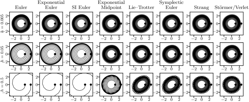
Figure 2. Numerical limit-cycle behavior ($x_{2}$ vs. $x_{1}$) for the Van der Pol oscillator with $\epsilon=0.05$. For the Euler-type methods, the limit cycle radius grows rapidly with $h$, consistent with Section 3.2.1. For the exponential midpoint method, this growth is negligible at smaller time steps but is clearly visible at $h=0.5$, consistent with Section 3.2.2. The splitting and composition methods exhibit much better limit-cycle preservation, consistent with Section 3.2.3; some skewing is visible for the first-order, non-symmetric Lie–Trotter and symplectic Euler methods.

Figure 2 shows phase portraits for three Euler-type methods (Euler, exponential Euler, and SI Euler), the exponential midpoint method, and four splitting/composition methods (Lie–Trotter splitting, symplectic Euler, Strang splitting, and Störmer/Verlet), applied to the Van der Pol oscillator with $\epsilon=0.05$. For the Euler-type methods, the numerical limit cycle radius is seen to grow with $h/\epsilon$, which is consistent with Section 3.2.1. For the exponential midpoint method, the $h^{3}/(4\epsilon)$ growth in limit cycle radius is less apparent at smaller time steps but is clearly visible at $h=0.5$, for which $h^{3}/(4\epsilon)=0.625$, consistent with Section 3.2.1. By contrast, for the non-symmetric and symmetric splitting and composition methods, there is no apparent growth in limit cycle radius—even when $h=0.5$, for which $h/\epsilon=10$—which is consistent with Section 3.2.3. Notice that the asymmetry and lower order of the Lie–Trotter splitting and symplectic Euler methods manifests as a skewing of the limit cycle for large $h$, while the limit cycle remains approximately circular for the symmetric methods.

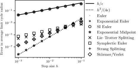
Figure 3. Error in average limit cycle radius for the Van der Pol oscillator with $\epsilon=0.05$ and various step sizes $h$. We see that the Euler-type methods have error $\sim h/\epsilon$, the exponential midpoint method has error $\sim h^{3}/(4\epsilon)$, the non-symmetric splitting/composition methods have error $\mathcal{O}(h)$, and the symmetric splitting/composition methods have error $\mathcal{O}(h^{2})$, consistent with the theoretical results.

Figure 3 illustrates how the average limit cycle radius converges, for each of these methods, as $h\rightarrow 0$. For the Euler-type methods, following Section 3.2.1, the error in average limit cycle radius is $\sim h/\epsilon$. For the exponential midpoint method, following Section 3.2.2, the error is $\sim h^{3}/(4\epsilon)$. For the splitting and composition methods, following Section 3.2.3, the error is $\mathcal{O}(h)$ for the non-symmetric methods and $\mathcal{O}(h^{2})$ for the symmetric methods.

Although the exponential midpoint method has the lowest error for small time steps, we make two remarks about this. First, this occurs because $h^{3}/\epsilon\ll h^{2}$ when $h\ll\epsilon$, which is more difficult to achieve when $\epsilon$ is even smaller. Second, since it requires twice as many function evaluations as the other methods, using the same computational budget would require time steps twice as large, roughly increasing the error by a constant factor of $8$.

3.3.2. Stiff Van der Pol oscillator

We next apply these methods to the Van der Pol oscillator with $\epsilon=50$. In contrast with the non-stiff case, we see notably different behavior among the three Euler-type methods, as well as between the splitting and composition methods of the same order.

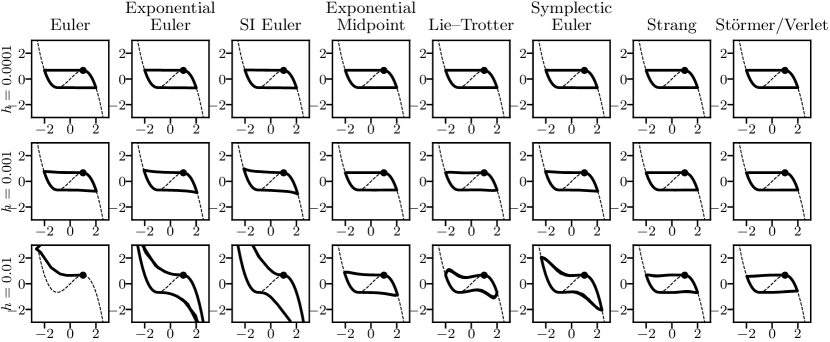
Figure 4. Numerical limit-cycle behavior ($y_{2}$ vs. $y_{1}$, cubic nullcline shown as dashed line) for the Van der Pol oscillator with $\epsilon=50$. As the time step size grows, the exponential midpoint and splitting/composition methods exhibit substantially less limit cycle distortion than the Euler-type methods (while Euler’s method itself becomes unstable), and the Lie–Trotter splitting method performs notably better than the symplectic Euler composition method of the same order.

Figure 4 shows numerical phase plots in the $(y_{1},y_{2})$ plane defined by the Liénard transformation introduced in Section 3.1. For $h=0.0001$, all methods show numerical limit cycles resembling the reference solution in Figure 1, with solutions “jumping” between branches of the cubic nullcline approximately horizontally at the critical values $y_{2}=\pm 2/3$. For the Euler-type methods, rather than remaining approximately horizontal as $h$ grows, these jumps grow in the direction of increasing $\lvert y_{2}\rvert$, resulting in instability for Euler’s method at $h=0.01$ and severe limit cycle distortion for the exponential Euler and SI Euler methods. The symplectic Euler method exhibits similar behavior, albeit less severely. Although the Lie–Trotter splitting method also shows limit cycle distortion, the jumps oscillate and return to the nullcline at nearly the correct points. The exponential midpoint and Störmer/Verlet methods both exhibit much less limit cycle distortion, with $\lvert y_{2}\rvert$ increasing slightly during jumps for the exponential midpoint method and decreasing slightly for the Störmer/Verlet method. The Strang splitting method also exhibits very little distortion and, like Lie–Trotter, appears to oscillate and return to the nullcline at nearly the correct point.

	$\lvert y_{1}\rvert$			$\lvert y_{2}\rvert$
$h$	0.0001	0.001	0.01	0.0001	0.001	0.01
Euler	2.01	2.03	——	0.68	0.77	——
Exponential Euler	2.01	2.07	3.18	0.69	0.88	7.52
SI Euler	2.01	2.10	4.34	0.70	0.99	22.82
Exponential Midpoint	2.00	2.00	2.07	0.68	0.68	0.87
Lie–Trotter	2.00	2.00	2.00	0.68	0.68	0.68
Symplectic Euler	2.01	2.03	2.37	0.68	0.77	2.06
Strang	2.00	2.00	2.00	0.68	0.68	0.68
Störmer/Verlet	2.00	2.00	1.97	0.68	0.67	0.57

Table 1. Values of $\lvert y_{1}\rvert$, $\lvert y_{2}\rvert$ at which numerical solutions return to the cubic nullcline after jumping, for the Van der Pol oscillator with $\epsilon=50$. These values increase with $h$ for the Euler-type methods, increase more modestly for the symplectic Euler method, increase slightly for the exponential midpoint method, and decrease slightly for the Störmer/Verlet method. The Lie–Trotter and Strang splitting methods exhibit no drift in these values at the level of precision shown.

Table 1 quantifies the observations made in the previous paragraph by showing the values of $\lvert y_{1}\rvert$, $\lvert y_{2}\rvert$ at which the jumps return to the nullcline. This is computed by finding the point $(y_{1},y_{2})$ along each numerical solution at which $\lvert y_{1}\rvert$ attains a maximum. For the Euler-type, exponential midpoint, and symplectic Euler methods, these values increase as $h$ increases, while Störmer/Verlet shows a small decrease. By contrast, the two splitting methods do not show any drift at the precision displayed.

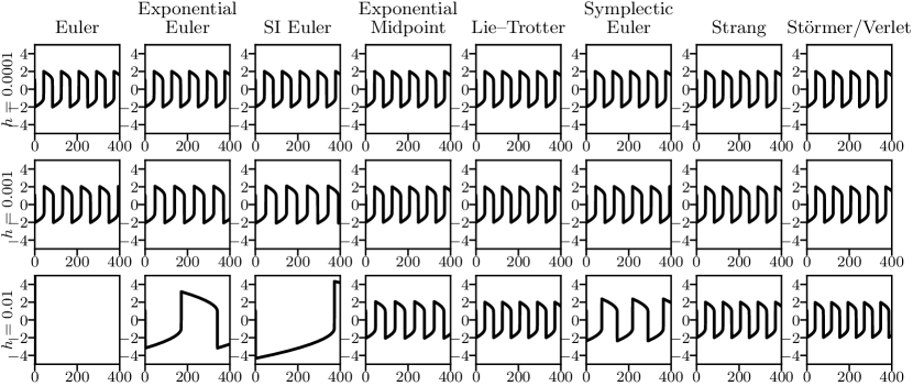
Figure 5. Numerical spiking behavior ($x_{1}$ vs. $t$) for the Van der Pol oscillator with $\epsilon=50$. As the time step size grows, Euler’s method becomes unstable, and the stable Euler-type methods exhibit a severe decrease in spike frequency and increase in spike amplitude. This frequency and amplitude drift is moderate for symplectic Euler and slight for exponential midpoint and Störmer/Verlet, while the splitting methods show no apparent drift in spiking behavior at all.

Figure 5 shows time plots for these same numerical solutions. As $h$ increases, the Euler-type methods show severely decreased spike frequency and increased spike amplitude. Symplectic Euler exhibits this same behavior less severely and exponential midpoint only slightly, while Störmer/Verlet exhibits a slight increase in spike frequency. By contrast, the Lie–Trotter and Strang splitting methods have no apparent change in spike frequency or amplitude.

This behavior is explained by the preceding observations about the points at which jumps return to the nullcline. For the stiff Van der Pol oscillator, jumps occur quickly, so nearly all of the time is spent moving slowly along the nullcline. Numerical solutions that return to the nullcline at too-large values of $\lvert y_{1}\rvert$, $\lvert y_{2}\rvert$ must spend more time moving along the nullcline between jumps, resulting in decreased spike frequency; this is the case for the Euler-type, symplectic Euler, and exponential midpoint methods. Likewise, those which return at too-small values of $\lvert y_{1}\rvert$, $\lvert y_{2}\rvert$ spend less time moving along the nullcline, resulting in increased spike frequency; this is the case for Störmer/Verlet. This also explains why the Lie–Trotter method preserves the correct spiking behavior, in spite of the limit cycle distortion observed in Figure 4: this distortion occurs almost entirely during the jumps, where the solution spends very little time.

4. Limit cycle preservation for Hodgkin–Huxley neurons

4.1. The Hodgkin–Huxley model

Based on electrophysiology experiments, Hodgkin and Huxley [15] proposed a model, consisting of a nonlinear system of partial differential equations, to describe the dynamics of the membrane potential of the squid giant axon. If the membrane potential is assumed to be uniform in space along the axon, the Hodgkin–Huxley model reduces to a conditionally linear system of ODEs:

(5) $$C\dot{V} =I-\bar{g}_{\mathrm{K}}n^{4}(V-E_{\mathrm{K}})-\bar{g}_{\mathrm{Na}}m^{3}h(V-E_{\mathrm{Na}})-\bar{g}_{\mathrm{L}}(V-E_{\mathrm{L}}),$$

$$\dot{n} =\alpha_{n}(V)(1-n)-\beta_{n}(V)n,$$

$$\dot{m} =\alpha_{m}(V)(1-m)-\beta_{m}(V)m,$$

$$\dot{h} =\alpha_{h}(V)(1-h)-\beta_{h}(V)h.$$

This describes how $V$, the voltage across a membrane with capacitance $C$, responds to an input current $I$. (In a neural network, $I$ depends on the membrane voltage of neighboring neurons connected by synapses. Therefore, a network of Hodgkin–Huxley neurons is also conditionally linear.) The constants $\bar{g}_{\mathrm{K}}$, $\bar{g}_{\mathrm{Na}}$, $\bar{g}_{\mathrm{L}}$ and $E_{\mathrm{K}}$, $E_{\mathrm{Na}}$, $E_{\mathrm{L}}$ are, respectively, the conductances and reversal potentials for the potassium (K), sodium (Na), and leak (L) channels. The other dynamical variables, $n$, $m$, $h$, are dimensionless auxiliary quantities between $0$ and $1$, corresponding to potassium channel activation, sodium channel activation, and sodium channel inactivation; $\alpha_{n}$, $\alpha_{m}$, $\alpha_{h}$ and $\beta_{n}$, $\beta_{m}$, $\beta_{h}$ are given rate functions of $V$.

For the remainder of this section, we take units of mV for $V$ and ms for $t$ and consider model neurons with the parameters

$$\bar{g}_{\mathrm{K}}=36,\quad\bar{g}_{\mathrm{Na}}=120,\quad\bar{g}_{\mathrm{L}}=0.3,\quad E_{\mathrm{K}}=-77,\quad E_{\mathrm{Na}}=55,\quad E_{\mathrm{L}}=-61,$$

and rate functions

$$\alpha_{n}(V) =\frac{0.01(10-65-V)}{\exp\bigl{(}\frac{10-65-V}{10}\bigr{)}-1}, \beta_{n}(V) =0.125\exp\biggl{(}\frac{-65-V}{80}\biggr{)},$$

$$\alpha_{m}(V) =\frac{0.1(25-65-V)}{\exp\bigl{(}\frac{25-65-V}{10}\bigr{)}-1}, \beta_{m}(V) =4\exp\biggl{(}\frac{-65-V}{18}\biggr{)},$$

$$\alpha_{h}(V) =0.07\exp\biggl{(}\frac{-65-V}{20}\biggr{)}, \beta_{h}(V) =\frac{1}{\exp\bigl{(}\frac{30-65-V}{10}\bigr{)}+1}.$$

These rate functions agree with those in Hodgkin and Huxley [15] with a resting potential of $-65$ mV.

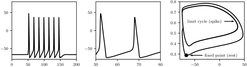
Figure 6. Reference solution for a single Hodgkin–Huxley neuron, showing voltage $V$ in mV as a function of time $t$ in ms (left), a zoomed-in view of the first two spikes (center), and the corresponding curve in the $(V,n)$ phase plane (right). An input current of 10 nA is switched on at $t=50$, causing the neuron to begin firing periodically, and is switched off again at $t=150$, causing it to return to a resting equilibrium. In the phase plane, the resting state corresponds to a fixed point, while the spiking state corresponds to a limit cycle. The outer loop in the phase portrait traces the transition between resting and spiking, including the large initial spike when the current is first switched on.

Figure 6 shows a reference solution to (5), illustrating the bifurcation and limit cycle behavior that governs neuronal spiking, as discussed in Section 1. Since the limit cycle lies on a two-dimensional center manifold (Hassard [12], Izhikevich [16]), these dynamics can be portrayed by projecting to a two-dimensional phase plot in the $(V,n)$ plane.

The limit cycle, together with a time parametrization, determines the shape of action potentials. Since we are interested in preserving these features, it is worth discussing the question: Is the shape of an action potential an important feature for a neuron model to capture? It has been well established that the shape of an action potential can and does vary between neurons. For example, regular-spiking pyramidal neuron action potentials are broader and differ detectably from the narrow, fast-spiking interneurons (Bean [1], Nowak et al. [25]). These differences are commonly exploited during extracellular recordings for identifying the neuron type; further, even for the same neuron, the shape of the action potential changes depending on whether the recording is made from axonal or somatic compartments [1]. Therefore, faithfully capturing this neural response feature would be important for modeling the diversity of cell types typically found in biological neural networks, and even for developing tightly constrained multi-compartment models of single neurons. For developing models of neural networks, the effect of the action potential on the post-synaptic neuron must be considered. The effect of an action potential from a pre-synaptic onto the post-synaptic neuron can differ depending on the type of synapses (chemical vs. electrical) between them (Destexhe et al. [6], Curti and O’Brien [5]). Would differences in action potential shapes, at the level of individual neurons, alter information processing and other emergent properties, such as neural synchronization, at a network level? This is not fully understood and is a direction for future investigation.

4.2. Application of numerical methods

Since (5) is conditionally linear, the application of Euler-type methods is straightforward; so is the application of other explicit exponential Runge–Kutta methods, such as the exponential midpoint method. The use of the exponential Euler method for Hodgkin–Huxley was proposed by Moore and Ramon [23], and it has since been in widespread use in computational neuroscience, including as the default numerical integrator in the GENESIS software package (Bower and Beeman [3]). Butera and McCarthy [4] showed that exponential Euler often gives larger errors than Euler’s method for moderately large time steps where both methods are stable. Börgers and Nectow [2], in addition to exponential Euler, also considered the SI Euler and exponential midpoint methods for Hodgkin–Huxley.

In order to apply the splitting and composition methods of Section 2.4 to Hodgkin–Huxley, we begin by splitting the vector field $f$ defining the right-hand side of (5) into

$$f=f^{(V)}+f^{(n)}+f^{(m)}+f^{(h)}.$$

However, the vector fields $f^{(n)}$, $f^{(m)}$, and $f^{(h)}$ commute, since when $V$ is held fixed, the variables $n$, $m$, $h$ evolve independently. Taking $f^{(n,m,h)}=f^{(n)}+f^{(m)}+f^{(h)}$, we have $\Phi_{h}^{(n,m,h)}=\Phi_{h}^{(n)}\circ\Phi_{h}^{(m)}\circ\Phi_{h}^{(h)}$ for any exact or approximate flow $\Phi_{h}$, and we can evolve these flows in parallel (see Section 2.4).

Therefore, in spite of the fact that (5) is four-dimensional, we can construct splitting and composition methods using only two flows. As before, we consider non-symmetric and symmetric splitting/composition methods:

$$\Phi_{h}^{(V)}\circ\Phi_{h}^{(n,m,h)},\qquad\Phi_{h/2}^{(n,m,h)\ast}\circ\Phi_{h/2}^{(V)\ast}\circ\Phi_{h/2}^{(V)}\circ\Phi_{h/2}^{(n,m,h)}.$$

Taking $\Phi_{h}^{(V)}=\varphi_{h}^{(V)}$ and $\Phi_{h}^{(n,m,h)}=\varphi_{h}^{(n,m,h)}$ to be the exact flows, the non-symmetric method is again the Lie–Trotter splitting method, and the symmetric method is the Strang splitting method. On the other hand, if we take $\Phi_{h}^{(V)}$ to be Euler’s method and $\Phi_{h}^{(n,m,h)}$ to be the backward Euler method, then we again refer to the resulting composition methods as symplectic Euler and Störmer/Verlet, respectively. We refer back to Section 2.4 and Section 2.4 for the explicit formulas for these methods.

As with the ${d}=2$ symmetric splitting/composition methods, we may reuse the nonlinear function evaluation from $\Phi_{h/2}^{(V)}$ for $\Phi_{h/2}^{(V)\ast}$, and likewise from $\Phi_{h/2}^{(n,m,h)\ast}$ for $\Phi_{h/2}^{(n,m,h)}$. Therefore, with the exception of the very first half-step of the symmetric method, both the non-symmetric and symmetric splitting/composition methods require only one evaluation of each nonlinear function per step, just as for the Euler-type methods.

Remark .

The Störmer/Verlet method can be seen as alternating between the time-$h$ flows $\Phi_{h/2}^{(V)\ast}\circ\Phi_{h/2}^{(V)}$ and $\Phi_{h/2}^{(n,m,h)}\circ\Phi_{h/2}^{(n,m,h)\ast}$, both of which correspond to the trapezoid method. If we ignore the half-steps, this can be seen as a staggered-grid method with $V$ stored at integer time steps and $(n,m,h)$ at half-integer time steps. This perspective, with $V$ and $(n,m,h)$ stored at staggered time steps and advanced using the trapezoid method, was suggested by Hines [13, Eq. 8] and later appeared in Mascagni and Sherman [18, p. 599–600].

The Störmer/Verlet formulation above has the advantage of producing values of $(V,n,m,h)$ all at integer time steps, rather than only at staggered time steps. A slightly different non-staggered formulation of Hines’ method was recently proposed by Hanke [11], using Euler’s method instead of backward Euler for $\Phi_{h/2}^{(n,m,h)}$.

4.3. Numerical experiments

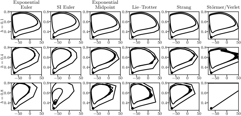
Figure 7. Numerical bifurcation and limit-cycle behavior for the Hodgkin–Huxley neuron in the $(V,n)$ phase plane. The exponential midpoint and splitting methods show better limit-cycle preservation (particularly with respect to shrinking in the $V$ direction) than the exponential Euler or (especially) SI Euler methods as $h$ increases, while the Störmer/Verlet method becomes numerically unstable.

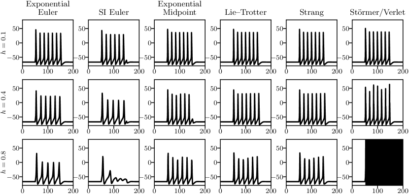
Figure 8. Numerical spiking behavior ($V$ in mV vs. $t$ in ms) for the Hodgkin–Huxley neuron, which is stimulated by a 10 nA input current between $t=50$ and $t=150$ ms. The Lie–Trotter and Strang splitting methods show less severe decrease in spiking frequency and amplitude than either the exponential Euler or (especially) SI Euler methods, and very slightly less than the exponential midpoint method. For example, both splitting methods emit the correct number of spikes, 7, at $h=0.4$, while exponential midpoint and exponential Euler emit 6 spikes and SI Euler only 5 spikes. The Störmer/Verlet method becomes numerically unstable.

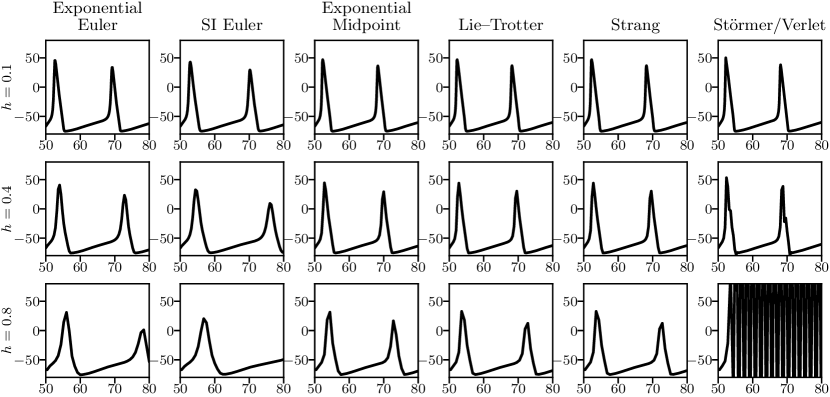
Figure 9. A zoomed-in view of the plots in Figure 8, showing the shape of the first two action potentials. For the exponential Euler method, the spikes become less sharp and more spread out as $h$ increases, and this effect is even worse for the SI Euler method. The exponential midpoint and splitting methods do a better job at preserving the shape and width of the spikes, while the Störmer/Verlet method becomes unstable for large $h$.

Figure 7, Figure 8, and Figure 9 show the results of applying Euler-type methods, the exponential midpoint method, and splitting/composition methods to the Hodgkin–Huxley system (5), with the parameters and rate functions specified in Section 4.1, for a range of large time step sizes. Euler’s method and the symplectic Euler method both exhibited numerical instability at these time step sizes, so they do not appear in the figures. The specific problem is the same one for which the reference solution appears in Figure 6: the neuron is simulated for 200 ms, with a constant 10 nA input current switched on at $t=50$ ms and switched off again at $t=150$ ms. The neuron is initially at rest, begins spiking after the input current is switched on, and returns to rest after the input current is switched off.

As they did for the stiff Van der Pol oscillator in Section 3.3.2, the exponential Euler and SI Euler methods exhibit limit cycle distortion and decreased spiking frequency as $h$ increases, and this is especially severe for the SI Euler method. For instance, notice that in the reference solution, the neuron fires 7 spikes in response to the input current. In Figure 8 the exponential Euler method fires 7 spikes at $h=0.1$, 6 spikes at $h=0.4$, and 5 spikes at $h=0.8$, while the SI Euler method fires only 6 spikes at $h=0.1$ and 5 spikes at $h=0.4$, and its spiking behavior is essentially damped away at $h=0.8$. Decreased spiking amplitude is also apparent, which corresponds to the limit cycle being compressed horizontally, as observed in Figure 7. Zooming in on the spikes, in Figure 9, we see that they become less sharp and more stretched out for these methods as $h$ increases.

By contrast, the Lie–Trotter and Strang splitting methods both appear to do a better job at preserving the limit cycle, as well as spiking frequency and amplitude, as $h$ increases. Both splitting methods fire 7 spikes at $h=0.1$ and $h=0.4$, and this decreases to 6 spikes at $h=0.8$. Some decrease in spiking amplitude is apparent at $h=0.8$, although at each step size there is less amplitude decay than for either the exponential Euler or SI Euler methods. Therefore, although some decrease in spiking frequency and amplitude occurs for the splitting methods, it appears to be notably less severe than for these other methods. Likewise, the spikes remain sharper and less stretched out for the splitting methods than for the Euler-type methods, although some smearing out of the spike shape is clearly visible at $h=0.8$.

The exponential midpoint method performs slightly worse than the splitting methods at the same time step size: it only fires 6 spikes at $h=0.4$, although it comes close to firing a 7th, and the spike amplitude exhibits fluctuations. At $h=0.8$, its decrease in spiking amplitude and frequency is comparable to that of the splitting methods. Preservation of spike shape is also similar to the splitting methods. However, since the exponential midpoint method requires twice as many function evaluations per step, one could use a splitting method with $h=0.4$ at the same cost as exponential midpoint with $h=0.8$, and by that comparison the splitting methods are clearly superior.

Finally, the Störmer/Verlet method—which, as we noted in Section 4.2, can be seen as a non-staggered version of Hines’ method [13]—becomes unstable as $h$ increases. Although it exhibits the correct behavior (both in terms of spiking frequency and amplitude) at $h=0.1$, the beginnings of instability are visible at $h=0.4$ in the increase and fluctuation in spiking amplitude, while the method has become unstable by $h=0.8$.

These experiments suggest that the Lie–Trotter and Strang splitting methods can preserve the correct spiking behavior in Hodgkin–Huxley neurons for larger time steps than can the exponential Euler or SI Euler methods—and the SI Euler method performs especially poorly in this regard. The exponential midpoint method performs similarly to the splitting methods but at twice the cost per time step; after normalizing for computational cost, the splitting methods come out on top. Methods involving Euler steps, including Euler’s method, symplectic Euler, and Störmer/Verlet, begin to suffer from numerical instability at these large time step sizes.

4.4. Remarks on reduced Hodgkin–Huxley models

The numerical experiments in Börgers and Nectow [2] do not actually simulate the full, four-dimensional Hodgkin–Huxley system (5). Rather, they make the simplifying assumption that sodium activation is “instantaneous,” so that $m=m_{\infty}(V)\coloneqq\alpha_{m}(V)/\bigl{(}\alpha_{m}(V)+\beta_{m}(V)\bigr{)}$, which eliminates the differential equation for $m$ and yields a three-dimensional reduced model. The reduced model is no longer conditionally linear, since $m_{\infty}(V)$ appears in the differential equation for $V$, but Börgers and Nectow [2] deal with this by freezing $m$ at the beginning of each step, including the intermediate step of exponential midpoint.

Because of the differences between the full Hodgkin–Huxley model and the reduced model, there are some discrepancies between the numerical results presented here and those in Börgers and Nectow [2], especially with regard to the decreasing amplitude of spikes at large time steps, which we observe and they do not. The purpose of this section is to briefly discuss these differences and to point out some of the dynamical changes that are introduced by using the reduced model.

The primary purpose of reducing the Hodgkin–Huxley model to two or three dimensions, by assuming instantaneous sodium activation and/or replacing $n$ and $h$ by a single variable, is to obtain a simpler system whose qualitative dynamics can be more easily analyzed. Meunier [22] compares the dynamics of these reduced models to those of Hodgkin–Huxley, observing several “spurious effects not displayed by the original models” that “arise mainly from the assumption that the variable $m$ follows instantaneously the variations of $V$,” and concludes that “taking into account properly the dynamics of sodium activation has more importance than choosing a reduction scheme or another for the slow variables.” While reduction is useful for understanding qualitative dynamics, he points out that “[i]f saving computation time was one of the reasons originally it is no longer of dominant importance” and “it is not meant to be used as a substitute to the original equations in network simulations.”

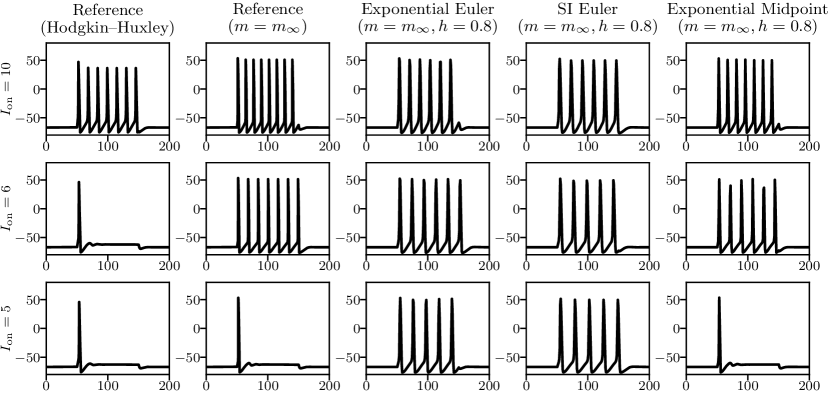
Figure 10. Treating sodium activation as instantaneous ($m=m_{\infty}$) results in different spiking behavior than in the original Hodgkin–Huxley model. For $I_{\text{on}}=10$, the Hodgkin–Huxley model emits 7 spikes, the first one larger than the other 6, whereas the $m=m_{\infty}$ model emits 8 large spikes of roughly the same amplitude. For $I_{\text{on}}=6$, the Hodgkin–Huxley model emits only one spike and returns to rest, whereas the $m=m_{\infty}$ model emits 7 large spikes. For $I_{\text{on}}=5$, both models emit only one spike. At $h=0.8$ ms, the Euler-type methods and exponential midpoint method exhibit decrease in spiking frequency—but not in amplitude, as they did with the full Hodgkin–Huxley model—and the Euler-type methods spike spuriously at $I_{\text{on}}=5$.

Figure 10 illustrates some of the “spurious effects” that can result from treating sodium activation as instantaneous, including spiking at subthreshold input currents. We perform the same numerical experiment as in Section 4.3, switching on an input current $I_{\text{on}}$ between $t=50$ and $t=150$ ms. In addition to $I_{\text{on}}=10$ nA, which was used in the previous experiments, we also consider currents of 6 nA and 5 nA, which are subthreshold for the original Hodgkin–Huxley model. Only the exponential Euler, SI Euler, and exponential midpoint methods of Börgers and Nectow [2] are shown, since the splitting/composition methods fundamentally require conditional linearity.

Finally, we remark that, in spite of its dynamical differences from Hodgkin–Huxley, this reduced model is widely used and useful. The exponential Euler, SI Euler, and exponential midpoint methods are well suited to it, whereas the splitting/composition methods are only applicable to the full Hodgkin–Huxley model. Whether or not to use instantaneous sodium activation is ultimately a modeling question rather than a numerical one, and it should not be used numerically if one actually wishes to simulate the full Hodgkin–Huxley dynamics.

5. Conclusion

For conditionally linear systems, such as the Van der Pol oscillator and Hodgkin–Huxley model of neuronal dynamics, the exponential Euler and SI Euler methods remain stable at much larger time step sizes than the classical Euler method, with no additional computational cost per step. However, we have shown that these Euler-type methods preserve the limit cycles of these systems poorly as the time step size grows, producing oscillations with the wrong amplitude and/or frequency. (This adds to previous observations about the inaccuracy of exponential Euler with large time steps for the Hodgkin–Huxley model, cf. Butera and McCarthy [4].) Since limit cycles underlie the dynamics of neuronal spiking, this is a serious problem for the use of Euler-type methods with large time steps.

By contrast, we have shown that splitting and composition methods exhibit better limit cycle preservation for these systems as time step size grows, with no additional cost per step. For the non-stiff Van der Pol oscillator, the (first-order, non-symmetric) Lie–Trotter splitting and symplectic Euler composition methods perform similarly, as do the (second-order, symmetric) Strang splitting and Störmer/Verlet methods. However, for the stiff Van der Pol oscillator and Hodgkin–Huxley models, the splitting methods both do a better job of preserving the frequency and amplitude of oscillations, and maintaining numerical stability, than the corresponding composition methods. With respect to these properties, the splitting methods are also seen to outperform the exponential midpoint method, which requires twice as many function evaluations per step.

Of all the methods considered, the Strang splitting method exhibits the best performance across the spectrum of non-stiff and stiff systems. This method also has the advantage of being second-order, although its order is not the main reason for its superior performance; this is evinced by the fact that the first-order Lie–Trotter splitting method performs nearly as well and outperforms the Euler-type methods having the same order. The Strang splitting method ought to be seriously considered as a competitor to exponential Euler as the “standard” integration method for such problems.

Although we have focused on the performance of these integrators for individual Hodgkin–Huxley neurons, future work should look at the implementation and performance of the Strang splitting method for networks of neurons. For large networks, Section 2.5 lays out a hybrid Euler-type/splitting approach by which such a system could be partitioned for efficient parallel implementation. Another direction for future work involves exponential integrators based on local linearization, such as the exponential Rosenbrock–Euler method (cf. Hochbruck and Ostermann [14]), rather than coordinate splitting.

Acknowledgments

Zhengdao Chen was supported in part by an ARTU research fellowship in the Department of Mathematics and Statistics at Washington University in St. Louis. Baranidharan Raman was supported in part through an NSF CAREER grant (#1453022). Ari Stern was supported in part by grants from the NSF (DMS-1913272) and from the Simons Foundation (#279968). We also wish to thank the anonymous referees for their helpful comments and suggestions.

References

- Bean [2007] B. P. Bean, The action potential in mammalian central neurons., Nat. Rev. Neurosci., 8 (2007), pp. 451–465.
- Börgers and Nectow [2013] C. Börgers and A. R. Nectow, Exponential time differencing for Hodgkin-Huxley-like ODEs, SIAM J. Sci. Comput., 35 (2013), pp. B623–B643.
- Bower and Beeman [1998] J. M. Bower and D. Beeman, The book of GENESIS, Springer-Verlag, New York, 1998.
- Butera and McCarthy [2004] R. J. Butera and M. L. McCarthy, Analysis of real-time numerical integration methods applied to dynamic clamp experiments, J. Neural Eng., 1 (2004), pp. 187–194.
- Curti and O’Brien [2016] S. Curti and J. O’Brien, Characteristics and plasticity of electrical synaptic transmission., BMC Cell Biol., 17 Suppl. 1 (2016), p. 13.
- Destexhe et al. [1994] A. Destexhe, Z. F. Mainen, and T. J. Sejnowski, Synthesis of models for excitable membranes, synaptic transmission and neuromodulation using a common kinetic formalism., J. Comput. Neurosci., 1 (1994), pp. 195–230.
- Fitzhugh [1961] R. Fitzhugh, Impulses and physiological states in theoretical models of nerve membrane, Biophys. J., 1 (1961), pp. 445–66.
- Hairer and Lubich [1999] E. Hairer and C. Lubich, Invariant tori of dissipatively perturbed Hamiltonian systems under symplectic discretization, Appl. Numer. Math., 29 (1999), pp. 57–71.
- Hairer and Lubich [2018] , Energy behaviour of the Boris method for charged-particle dynamics, BIT Numer. Math., (2018). In press, available at https://doi.org/10.1007/s10543-018-0713-1.
- Hairer et al. [2006] E. Hairer, C. Lubich, and G. Wanner, Geometric numerical integration, vol. 31 of Springer Series in Computational Mathematics, Springer-Verlag, Berlin, second ed., 2006. Structure-preserving algorithms for ordinary differential equations.
- Hanke [2017] M. Hanke, On a variable step size modification of Hines’ method in computational neuroscience, 2017. arXiv:1702.05917 [math.NA].
- Hassard [1978] B. Hassard, Bifurcation of periodic solutions of the Hodgkin–Huxley model for the squid giant axon, J. Theor. Biol., 71 (1978), pp. 401–420.
- Hines [1984] M. Hines, Efficient computation of branched nerve equations, Int. J. Biomed. Comput., 15 (1984), pp. 69–76.
- Hochbruck and Ostermann [2010] M. Hochbruck and A. Ostermann, Exponential integrators, Acta Numer., 19 (2010), pp. 209–286.
- Hodgkin and Huxley [1952] A. L. Hodgkin and A. F. Huxley, A quantitative description of membrane current and its application to conduction and excitation in nerve, J. Physiol., 117 (1952), pp. 500–544.
- Izhikevich [2007] E. M. Izhikevich, Dynamical systems in neuroscience: the geometry of excitability and bursting, Computational Neuroscience, MIT Press, Cambridge, MA, 2007.
- Liénard [1928] A.-M. Liénard, Etude des oscillations entretenues, Rev. Gen. Electr., 23 (1928), pp. 901–912, 946–954.
- Mascagni and Sherman [1998] M. V. Mascagni and A. S. Sherman, Numerical methods for neuronal modeling, in Methods in neuronal modeling: from ions to networks, C. Koch and I. Segev, eds., Computational Neuroscience, MIT Press, Cambridge, MA, second ed., 1998, pp. 569–606.
- McLachlan [1995] R. I. McLachlan, On the numerical integration of ordinary differential equations by symmetric composition methods, SIAM J. Sci. Comput., 16 (1995), pp. 151–168.
- McLachlan and Quispel [2002] R. I. McLachlan and G. R. W. Quispel, Splitting methods, Acta Numer., 11 (2002), pp. 341–434.
- McLachlan and Stern [2014] R. I. McLachlan and A. Stern, Modified trigonometric integrators, SIAM J. Numer. Anal., 52 (2014), pp. 1378–1397.
- Meunier [1992] C. Meunier, Two and three dimensional reductions of the Hodgkin–Huxley system: separation of time scales and bifurcation schemes, Biol. Cybernet., 67 (1992), pp. 461–468.
- Moore and Ramon [1974] J. W. Moore and F. Ramon, On numerical integration of the Hodgkin and Huxley equations for a membrane action potential, J. Theor. Biol., 45 (1974), pp. 249–273.
- Nagumo et al. [1962] J. Nagumo, S. Arimoto, and S. Yoshizawa, An active pulse transmission line simulating nerve axon, Proc. IRE, 50 (1962), pp. 2061–2070.
- Nowak et al. [2003] L. G. Nowak, R. Azouz, M. V. Sanchez-Vives, C. M. Gray, and D. A. McCormick, Electrophysiological classes of cat primary visual cortical neurons in vivo as revealed by quantitative analyses., J. Neurophysiol., 89 (2003), pp. 1541–1566.
- Stern and Grinspun [2009] A. Stern and E. Grinspun, Implicit-explicit variational integration of highly oscillatory problems, Multiscale Model. Simul., 7 (2009), pp. 1779–1794.
- Stoffer [1998] D. Stoffer, On the qualitative behaviour of symplectic integrators. III. Perturbed integral systems, J. Math. Anal. Appl., 217 (1998), pp. 521–545.
- Strang [1968] G. Strang, On the construction and comparison of difference schemes, SIAM J. Numer. Anal., 5 (1968), pp. 506–517.
- Suzuki [1990] M. Suzuki, Fractal decomposition of exponential operators with applications to many-body theories and Monte Carlo simulations, Phys. Lett. A, 146 (1990), pp. 319–323.
- Trotter [1959] H. F. Trotter, On the product of semi-groups of operators, Proc. Amer. Math. Soc., 10 (1959), pp. 545–551.
- van der Pol [1926] B. van der Pol, On “relaxation-oscillations”, The London, Edinburgh, and Dublin Phil. Mag. and J. of Sci., 2 (1926), pp. 978–992.
- Yoshida [1990] H. Yoshida, Construction of higher order symplectic integrators, Phys. Lett. A, 150 (1990), pp. 262–268.
- Yoshida [1993] , Recent progress in the theory and application of symplectic integrators, Celestial Mech. Dynam. Astronom., 56 (1993), pp. 27–43. Qualitative and quantitative behaviour of planetary systems (Ramsau, 1992).