Time-dependent Darboux (supersymmetric) transformations for non-Hermitian quantum systems

Abstract:

We propose time-dependent Darboux (supersymmetric) transformations that provide a scheme for the calculation of explicitly time-dependent solvable non-Hermitian partner Hamiltonians. Together with two Hermitian Hamilitonians the latter form a quadruple of Hamiltonians that are related by two time-dependent Dyson equations and two intertwining relations in form of a commutative diagram. Our construction is extended to the entire hierarchy of Hamiltonians obtained from time-dependent Darboux-Crum transformations. As an alternative approach we also discuss the intertwining relations for Lewis-Riesenfeld invariants for Hermitian as well as non-Hermitian Hamiltonians that reduce the time-dependent equations to auxiliary eigenvalue equations. The working of our propsals is discussed for a hierarchy of explicitly time-dependent rational, hyperbolic, Airy function and nonlocal potentials.

1 Introduction

Darboux transformations [1] are very efficient tools in the study of exactly or quasi-exactly solvable systems. Formally they map solutions and coefficient functions of a partial differential equation to new solutions and a differential equation of similar form with different coefficient functions. The classic example is a second order differential equation of Sturm-Liouville type or time-independent Schrödinger equation (TDSE). Since in this context the Darboux transformation relates two operators that can be identified as isospectral Hamiltonians, this scenario has been interpreted as the quantum mechanical analogue of supersymmetry [2, 3, 4]. Many potentials with direct physical applications may be generated with this technique, such as for instance complex crystals with invisible defects [5, 6]. By relating quantum mechanical systems to soliton solutions of nonlinear differential equations, such as for instance the Korteweg-de Vries equation, the sine-Gordon equation or the nonlinear Schrödinger equation, Darboux transformations have also been very efficiently utilized in the construction of multi-soliton solutions [7, 8, 9, 10, 11].

Initially Darboux transformations were developed for stationary equations, so that the treatment of the full TDSE was not possible. Evidently the latter is a much more intricate problem to solve, especially for non-autonomous Hamiltonians. Explicitly time-dependent Darboux transformations for TDSE, rather than the time-independent Schrödinger equation, were first introduced by Bagrov and Samsonov [12] and subsequently generalized to other types of time-dependent systems [13, 14]. The limitations of the generalization from the time-independent to the time-dependent Schrödinger equation were that the solutions considered in [12] force the Hamiltonians involved to be Hermitian. One of the central purposes of this manuscript is to overcome this shortcoming and propose fully time-dependent Darboux transformations that deal directly with the TDSE involving non-Hermitian Hamiltonians. We extend our analysis to the entire hierarchy of solvable time-dependent Hamiltonians constructed from generalized versions of Darboux-Crum transformations. As an alternative scheme we also discuss the intertwining relations for Lewis-Riesenfeld invariants for Hermitian as well as non-Hermitian Hamiltonians. These quantities are constructed as auxiliary objects to convert the fully TDSE into an eigenvalue equation that is easier to solve and subsequently allows to tackle the TDSE. The class of non-Hermitian Hamiltonians we consider here is the one of $\mathcal{PT}$-symmetric/quasi-Hermitian ones [15, 16, 17] that are related to a Hermitian counterpart by means of the time-dependent Dyson equation (TDDE) [18, 19, 20, 21, 22, 23, 24, 25, 26, 27, 28].

Given the interrelations of the various quantities in the proposed scheme one may freely choose different initial starting points. A quadruple of Hamiltonians, two Hermitian and two non-Hermitian ones, is related by two TDDE and two intertwining relations in form of a commutative diagram. This allows to compute all four Hamiltonians by solving either two intertwining relations and one TDDE or one intertwining relations and two TDDE, with the remaining relation being satisfied by the closure of the commutative diagram. We discuss the working of our proposal by taking two concrete non-Hermitian systems as our starting points, the Gordon-Volkov Hamiltonian with a complex electric field and a reduced version of the Swanson model. From the various solutions to the TDSE we construct explicitly time-dependent rational, hyperbolic, Airy function and nonlocal potentials.

Our manuscript is organized as follows: In section 2 we review the time-dependent Darboux transformations for Hermitian Hamiltonians and stress the limitations of previous results. We propose a new scheme that allows for the treatment of non-Hermitian Hamiltonians. Subsequently we extend the Darboux transformations to Darboux-Crum transformations, that is we construct two hierarchies from intertwining operators build from solutions previously ignored. In section 3 we discuss the intertwining relations for Lewis-Riesenfeld invariants. Taking a complex Gordon-Volkov Hamiltonian as starting point we discuss in section 4 various options of how to close the commutative diagrams constructing the intertwining operators from different types of solutions for rational, hyperbolic, Airy function potentials. In section 5 we start from a reduced version of the Swanson model and carry out the analysis for two different Dyson maps. In addition we discuss intertwining relations for Lewis-Riesenfeld invariants for this concrete system. The solutions to the TDSE discussed in this section depend on the solutions of an auxiliary equation known as the dissipative Ermakov-Pinney equation. We discuss in appendix A how to obtain explicit solutions to this nonlinear second order differential equation. Our conclusions are stated in section 6.

2 Time-dependent Darboux-Crum transformations

2.1 Time-dependent Darboux transformations for Hermitian systems

Before introducing the time-dependent Darboux transformations for non-Hermitian systems we briefly recall the construction for the Hermitian setting. This revision will not only establish our notation, but it also serves to highlight why previous suggestions are limited to the treatment of Hermitian systems. Here we wish to overcome this shortcoming and extend the theory of Darboux transformations to include the treatment of time-dependent non-Hermitian Hamiltonians. Our main emphasis is on non-Hermitian systems that belong to the class of $\mathcal{PT}$-symmetric Hamiltonians, i.e. they remain invariant under the antilinear transformation $\mathcal{PT}:$ $x\rightarrow-x$, $p\rightarrow p$, $i\rightarrow-i$. Such type of systems are of physical interest as potentially they possess energy operators with real instantaneous eigenvalues, that are different from the Hamiltonians in the non-Hermitian case.

The time-dependent Hermitian intertwining relation introduced in [12] reads

$$\ell\left(i\partial_{t}-h_{0}\right)=\left(i\partial_{t}-h_{1}\right)\ell,$$ (1)

where the Hermitian Hamiltonians $h_{0}$ and $h_{1}$ involve explicitly time-dependent potentials $v_{j}\left(x,t\right)$

$$h_{j}\left(x,t\right)=p^{2}+v_{j}\left(x,t\right),\qquad j=0,1.$$ (2)

The intertwining operator $\ell$ is taken to be a first order differential operator

$$\ell\left(x,t\right)=\ell_{0}\left(x,t\right)+\ell_{1}\left(x,t\right)\partial_{x}.$$ (3)

In general we denote by $\phi_{j}$, $j=0,1$, the solutions to the two partner TDSEs $i\partial_{t}\phi_{j}=h_{j}\phi_{j}$. Throughout our manuscript we use the convention $\hbar=1$. Taking a specific solution $u(x,t):=\phi_{0}(x,t)$ to one of these equations, the constraints imposed by the intertwining relation (1) can be solved by

$$\ell_{1}\left(x,t\right)=\ell_{1}\left(t\right),\quad\ell_{0}\left(x,t\right)=-\ell_{1}\frac{u_{x}}{u},\quad v_{1}=v_{0}+i\frac{\left(\ell_{1}\right)_{t}}{\ell_{1}}+2\left(\frac{u_{x}}{u}\right)^{2}-2\frac{u_{xx}}{u},$$ (4)

where, as indicated, $\ell_{1}$ must be an arbitrary function of $t$ only. At this point the new potential $v_{1}$ might still be complex. However, besides mapping the coefficient functions, the main practical purpose of the Darboux transformations is that one also obtains exact solutions $\phi_{1}$ for the partner TDSE $i\partial_{t}\phi_{1}=h_{1}\phi_{1}$ by employing the intertwining operator. In this case the direct application, that is acting with (1) on $u$, yields just the trivial solution $\phi_{1}=lu=0$. For this reason different types of nontrivial solutions were proposed in [12]

$$\hat{\phi}_{1}=\frac{1}{\ell_{1}u^{\ast}},\qquad\text{and\qquad}\tilde{\phi}_{1}=\hat{\phi}_{1}\int^{x}\left|u\right|^{2}dx^{\prime},$$ (5)

which require, however, that one imposes

$$\ell_{1}(t)=\exp\left[-\int^{t}\mathop{\mathrm{I}m}\left(v_{0}+2\left(\frac{u_{x}}{u}\right)^{2}-2\frac{u_{xx}}{u}\right)dt^{\prime}\right].$$ (6)

It is this assumption on the particular form of the solution that forces the new potentials in the proposal of [12] to be real $v_{1}=\mathop{\mathrm{R}e}\left(v_{0}+2\left(u_{x}/u\right)^{2}-2u_{xx}/u\right)$. Notice that one might not be able to satisfy (6), as the right hand side must be independent of $x$. If the latter is not the case, the solutions in (5) and the partner Hamiltonian $h_{1}$ do not exist.

Here we also identify another type of nontrivial solutions. Acting with equation (1) to the right on a solution of the TDSE $i\partial_{t}\phi_{0}=h_{0}\phi_{0}$, say $\phi_{0}=\tilde{u}$, that is linearly independent from $\phi_{0}=u$ used in the construction of the intertwining operator will in general lead to nontrivial solutions

$$\phi_{1}=\mathcal{L}\left[u\right](\tilde{u}),\quad\text{with \ }\mathcal{L}\left[u\right](f):=\ell_{1}\left(t\right)\left(\partial_{x}f-\frac{u_{x}}{u}f\right)$$ (7)

to the second TDSE $i\partial_{t}\phi_{1}=h_{0}\phi_{1}$. This type of solution and was overlooked in [12] and in principle might lead to complex potentials $v_{1}$ as it is not restricted by any additional constraints.

2.2 Time-dependent Darboux transformations for non-Hermitian systems

In order to extend the previous analysis in the way that allows for other types of complex potentials, and especially general non-Hermitian Hamiltonians that are $\mathcal{PT}$-symmetric/quasi-Hermitian [15, 16, 17], we make use of the time-dependent Dyson equation (TDDE) [18, 19, 20, 21, 22, 23, 24, 25, 26, 27, 28] for both time-dependent Hermitian Hamiltonians $h_{0}(t)$, $h_{1}(t)$ and the time-dependent non-Hermitian Hamiltonians $H_{0}(t)$, $H_{1}(t)$

$$h_{j}=\eta_{j}H_{j}\eta_{j}^{-1}+i\partial_{t}\eta_{j}\eta_{j}^{-1},\qquad j=0,1.$$ (8)

The time-dependent Dyson maps $\eta_{j}(t)$ relate the solutions of the TDSE $i\partial_{t}\psi_{j}=H_{j}\psi_{j}$ to the previous ones for $\phi_{j}$ as

$$\phi_{j}=\eta_{j}\psi_{j},\qquad j=0,1.$$ (9)

Using (8) in the intertwining relation (1) yields

$$\ell\left(i\partial_{t}-\eta_{0}H_{0}\eta_{0}^{-1}-i\partial_{t}\eta_{0}\eta_{0}^{-1}\right)=\left(i\partial_{t}-\eta_{1}H_{1}\eta_{1}^{-1}-i\partial_{t}\eta_{1}\eta_{1}^{-1}\right)\ell.$$ (10)

Multiplying (10) from the left by $\eta_{1}^{-1}$ and acting to the right on $\eta_{0}f$, with $f(x,t)$ being some arbitrary test function, we obtain

$$\eta_{1}^{-1}\ell\left[i\left(\partial_{t}\eta_{0}\right)f+i\eta_{0}\partial_{t}f-\eta_{0}H_{0}f-i\left(\partial_{t}\eta_{0}\right)f\right]=$$

$$\left(i\eta_{1}^{-1}\ell\eta_{0}\partial_{t}f+i\eta_{1}^{-1}\left(\partial_{t}\ell\eta_{0}\right)f-H_{1}\eta_{1}^{-1}\ell\eta_{0}f-i\eta_{1}^{-1}\left(\partial_{t}\eta_{1}\right)\eta_{1}^{-1}\ell\eta_{0}f\right).$$ (11)

Rearranging the time derivative terms and removing the test function, we derive the new intertwining relation for non-Hermitian Hamiltonians

$$L\left(i\partial_{t}-H_{0}\right)=\left(i\partial_{t}-H_{1}\right)L,$$ (12)

where we introduced the new intertwining operator

$$L:=\eta_{1}^{-1}\ell\eta_{0}.$$ (13)

We note that $H_{j}-p^{2}$ is in general not only no longer real and might also include a dependence on the momenta, i.e. $H_{j}$ does not have to be a potential Hamiltonian and could be nonlocal. Denoting by $\psi_{0}=U=\eta_{0}^{-1}u~{}$a particular solution to the TDSE for $H_{0}$, the standard new solution $\psi_{1}=LU=\eta_{1}^{-1}\ell\eta_{0}\eta_{0}^{-1}u$ remains trivial. The nontrivial solutions (5) generalize to

$$\hat{\psi}_{1}=\eta_{1}^{-1}\frac{1}{\ell_{1}\left(\eta_{0}U\right)^{\ast}},\qquad\text{and\qquad}\tilde{\psi}_{1}=\hat{\psi}_{1}\int^{x}\left|\eta_{0}U\right|^{2}dx^{\prime}.$$ (14)

The nontrivial solution (7) becomes

$$\psi_{1}=L\left[U\right]\left(\tilde{U}\right)$$ (15)

in the non-Hermitian case. In summary, our quadruple of Hamiltonians is related as depicted in the commutative diagram

$$\begin{array}[]{ccccc}&H_{0}&~{}~{}\underrightarrow{\eta_{0}}{}{}&h_{0}&\\ \eta_{1}^{-1}\mathcal{L}\left[u\right]\eta_{0}&\downarrow&&\downarrow&\mathcal{L}\left[u\right]\\ &H_{1}&\underrightarrow{\eta_{1}}&h_{1}&\end{array}$$ (16)

One may of course also try to solve the intertwining relation (12) directly and build the intertwining operator $L$ from a solution $U=\eta_{0}^{-1}u$ for the TDSE for $H_{0}$ and ignore initially the fact that the Hamiltonians $H_{0}$ and $H_{1}$ involved are non-Hermitian. To make sense of these Hamiltonians one still needs to construct the Dyson maps $\eta_{0}$ and $\eta_{1}$. Considering the diagram

$$\begin{array}[]{ccccc}&H_{0}&~{}~{}\underrightarrow{\eta_{0}}{}{}&h_{0}&\\ \mathcal{L}\left[U\right]&\downarrow&&\downarrow&\mathcal{L}\left[u\right]\\ &H_{1}&\underrightarrow{?}&h_{1}&\end{array}$$ (17)

in which the TDDE has been solved for $\eta_{0}$, $H_{0}$, $h_{0}$ and $H_{1}$, $h_{1}$ have been constructed with intertwining operators build from the solutions of the respective TDSE, we address the question of whether it is possible to close the diagram, that is making it commutative. For this to be possible we require

$$\mathcal{L}\left[U\right]=\eta_{1}^{-1}\mathcal{L}\left[u\right]\eta_{0}$$ (18)

to be satisfied. It is easy to verify that (18) holds if and only if

$$\eta_{1}\mathcal{=}\eta_{0},\qquad\text{and\qquad}\frac{\eta_{0}^{-1}u_{x}}{\eta_{0}^{-1}u}=\eta_{0}^{-1}\frac{u_{x}}{u}\eta_{0}.$$ (19)

A solution for the second equation in (19) is for instance $\eta_{0}=f(x)T_{\alpha}(x)$, with $T_{\alpha}=e^{i\alpha p}$ being a standard shift operator, i.e. $T_{\alpha}g(x)=g(x+\alpha)$, and $f(x)$ an arbitrary $x$-dependent function.

2.3 Time-dependent Darboux-Crum transformations for Hermitian systems

Next we demonstrate that the iteration procedure of the Darboux transformation, usually referred to as Darboux-Crum (DC) transformations [1, 29, 7], will lead also in the time-dependent case to an entire hierarchy of exactly solvable time-dependent Hamiltonians $h_{0}$, $h_{1}$, $h_{2}$, … for the TDSEs $i\partial_{t}\phi^{(n)}=h_{n}\phi^{(n)}$ related to each other by intertwining operators $\ell^{(n)}$

$$\ell^{(n)}\left(i\partial_{t}-h_{n-1}\right)=\left(i\partial_{t}-h_{n}\right)\ell^{(n)},\qquad n=1,2,\ldots$$ (20)

For $n=1$ this is equation (1) with $\ell=\ell^{(1)}$ and solutions $\phi_{0}=\phi^{(0)}$, $\phi_{1}=\phi^{(1)}$. Taking a particular solution $\phi_{0}=u$ to depend on some parameter $\gamma$, continuously or discretely, we denote the solutions at different values as $u_{i}:=u(\gamma_{i})$. Given now $\ell^{(1)}=\mathcal{L}\left[u_{0}\right]$ from (3) we act with (20) for $n=1$ on $u_{1}$, so that we can cast the intertwining operator and the solution (7) in the form

$$\ell^{(1)}(f)=\mathcal{L}\left[u_{0}\right](f)=\ell_{1}\left(t\right)\frac{W_{2}[u_{0},f]}{W_{1}[u_{0}]},\quad\qquad\phi^{(1)}=\ell^{(1)}(u_{1})=\mathcal{L}\left[u_{0}\right](u_{1}),$$ (21)

with corresponding time-dependent Hamiltonian

$$h_{1}=h_{0}-2\left[\ln W_{1}(u_{0})\right]_{xx}+i\left[\ln\ell_{1}\right]_{t}.$$ (22)

We employed here the Wronskian $W_{n}[u_{1},u_{2},\ldots,u_{n}]:=$ $\det\omega$ with $\omega_{jk}=\partial^{j-1}u_{k}/\partial x^{j-1}$ for $j,k=1,\ldots,n$, e.g. $W_{1}[u_{0}]=$ $u_{0}$, $W_{2}[u_{0},u_{1}]=$ $u_{0}\left(u_{1}\right)_{x}-u_{1}\left(u_{0}\right)_{x}$, etc., which allows to write the expressions for the intertwining operator and Hamiltonians in the hierarchy in a very compact form. Iterating these equations we obtain the compact closed form for the intertwining operator

$$\ell^{(n)}(f) = \mathcal{L}\left[\ell^{(n-1)}(u_{n-1})\right](\ell^{(n-1)}(f))$$ (23)

$$= \ell_{1}^{n}\left(t\right)\frac{W_{n+1}[u_{0},u_{1},\ldots,u_{n-1},f]}{W_{n}[u_{0},u_{1},\ldots,u_{n-1}]}$$ (24)

$$= \ell_{1}^{n}\left(t\right)\left|\Omega\right|_{(n+1)(n+1)},$$ (25)

where $\left|\Omega\right|_{(n+1)(n+1)}$ denotes a quasideterminant [30] for the (n+1)$\times$(n+1)-matrix $\Omega$ with $\Omega_{jk}=\partial^{j-1}u_{k}/\partial x^{j-1}$, $\Omega_{j(n+1)}=\partial^{j-1}f/\partial x^{j-1}$ for $j=1,\ldots,n+1$, $k=1,\ldots,n$. For the time-dependent Hamiltonians we derive

$$h_{n}=h_{0}-2\left[\ln W_{n}\left(u_{0},u_{1},\ldots,u_{n-1}\right)\right]_{xx}+in\left(\ln\ell_{1}\right)_{t}.$$ (26)

Nontrivial solutions of the type (7) to the related TDSE $i\partial_{t}\phi^{(n)}=h_{n}\phi^{(n)}$ are then obtained as

$$\phi^{(n)}=\ell^{(n)}(u_{n})\text{.}$$ (27)

Instead of using the same solution $u_{i}$ of the TDSE for $h_{0}$ at different parameter values in the closed expression, it is also possible to replace some of the solutions $u_{i}$ by the second linear independent solutions $\tilde{u}_{i}$ at the same parameter values, see e.g. [31, 9, 32] and references therein for details. This choice allows for the treatment of degenerate solutions. Closed expressions for DC-transformation build from the solutions (14) can be found in [12]. Below we will illustrate the working of the formulae in this section with concrete examples.

2.4 Time-dependent DC transformations for non-Hermitian systems

The iteration procedure for the non-Hermitian system goes along the same lines as for the Hermitian case, albeit with different intertwining operators $L$. The iterated systems are

$$L^{(n)}\left(i\partial_{t}-H_{n-1}\right)=\left(i\partial_{t}-H_{n}\right)L^{(n)},\qquad n=1,2,\ldots$$ (28)

The intertwining operators read in this case

$$L^{(n)}(f)=\mathcal{L}\left[L^{(n-1)}(U_{n-1})\right](L^{(n-1)}(f))=\ell_{1}^{n}\left(t\right)\frac{W_{n+1}[U_{0},U_{1},\ldots,U_{n-1},f]}{W_{n}[U_{0},U_{1},\ldots,U_{n-1}]},$$ (29)

and the time-dependent Hamiltonians are

$$H_{n}=H_{0}-2\left[\ln W_{n}[U_{0},U_{1},\ldots,U_{n-1}]\right]_{xx}+in\left[\ln\ell_{1}\right]_{t}.$$ (30)

The nontrivial solutions to the related TDSE are then obtained as

$$\psi^{(n)}=L^{(n)}(U_{n}).$$ (31)

Notice that in (28)-(31) the only Dyson maps involved are $\eta_{0}$ and $\eta_{1}$. Alternatively we can also express $L^{(n)}=\eta_{n}^{-1}l^{(n)}\eta_{n-1}$ and $\psi^{(n)}=\eta_{n}^{-1}\phi^{(n)}$, but the computation of the $\eta_{n}$ for $n>1$ is not needed. Since the solutions (14) require the Hamiltonians involved to be Hermitian, hierarchies build on them do not exist in the non-Hermitian case.

3 Intertwining relations for Lewis-Riesenfeld invariants

As previously argued [33, 26, 28], the most efficient way to solve the TDDE (8), as well as the TDSE, is to employ the Lewis-Riesenfeld invariants [34]. The steps in this approach consists of first solving the evolution equation for the invariants of the Hermitian and non-Hermitian system separately and subsequently constructing a similarity transformation between the two invariants. By construction the map facilitating this transformation is the Dyson map satisfying the TDDE.

Here we need to find four time-dependent invariants $I_{j}^{h}(t)$ and $I_{j}^{H}(t)$, $j=0,1$, that solve the equations

$$\partial_{t}I_{j}^{H}(t)=i\left[I_{j}^{H}(t),H_{j}(t)\right],\quad\text{and\quad}\partial_{t}I_{j}^{h}(t)=i\left[I_{j}^{h}(t),h_{j}(t)\right]\text{.}$$ (32)

The solutions $\phi_{j}(t)$, $\psi_{j}(t)$ to the respective TDSEs are related by a phase factor $\left|\phi_{j}(t)\right\rangle=e^{i\alpha_{j}(t)}\left|\check{\phi}_{j}(t)\right\rangle$, $\left|\psi_{j}(t)\right\rangle=e^{i\alpha_{j}(t)}\left|\check{\psi}_{j}(t)\right\rangle$ to the eigenstates of the invariants

$$I_{j}^{h}(t)\left|\check{\phi}_{j}(t)\right\rangle=\Lambda_{j}\left|\check{\phi}_{j}(t)\right\rangle,~{}~{}~{}~{}~{}~{}~{}I_{j}^{H}(t)\left|\check{\psi}_{j}(t)\right\rangle=\Lambda_{j}\left|\check{\psi}_{j}(t)\right\rangle,~{}~{}~{}~{}~{}~{}~{}\text{with }\dot{\Lambda}_{j}=0.$$ (33)

Subsequently the phase factors can be computed from

$$\dot{\alpha}_{j}=\left\langle\check{\phi}_{j}(t)\right|i\partial_{t}-h_{j}(t)\left|\check{\phi}_{j}(t)\right\rangle=\left\langle\check{\psi}_{j}(t)\right|\eta_{j}^{\dagger}(t)\eta_{j}(t)\left[i\partial_{t}-H_{j}(t)\right]\left|\check{\psi}_{j}(t)\right\rangle.$$ (34)

As has been shown [33, 26, 28], the two invariants for the Hermitian and non-Hermitian system obeying the TDDE are related to each other by a similarity transformation

$$I_{j}^{h}=\eta_{j}I_{j}^{H}\eta_{j}^{-1}\text{.}$$ (35)

Here we show that the invariants $I_{0}^{H}$, $I_{1}^{H}$ and $I_{0}^{h}$, $I_{1}^{h}$ are related by the intertwining operators $L$ in (13) and $\ell$ in (3), respectively. We have

$$LI_{0}^{H}=I_{1}^{H}L,\qquad\text{and}\qquad\ell I_{0}^{h}=I_{1}^{h}\ell.$$ (36)

This is seen from computing

$$i\partial_{t}\left(LI_{0}^{H}-I_{1}^{H}L\right)=H_{1}\left(LI_{0}^{H}-I_{1}^{H}L\right)-\left(LI_{0}^{H}-I_{1}^{H}L\right)H_{0},$$ (37)

where we used (12) and (32) to replace time-derivatives of $L$ and $I_{0}^{H}$, respectively. Comparing (37) with (12) in the form $i\partial_{t}L=H_{1}L-LH_{0}$, we conclude that $L=LI_{0}^{H}-I_{1}^{H}L$ or $LI_{0}^{H}=I_{1}^{H}L$. The second relation in (36) follows from the first when using (13) and (35). Thus schematically the invariants are related in the same manner as depicted for the Hamiltonians in (16) with the difference that the TDDE is replaced by the simpler adjoint action of the Dyson map. Given the above relations we have no obvious consecutive orderings of how to compute the quantities involved. For convenience we provide a summary of the above in the following diagram to illustrate schematically how different quantities are related to each other:

Figure 1: Schematic representation of Dyson maps $\eta_{0}$,$\eta_{1}$ and intertwining operators $\ell$,$L$ relating quadruples of Hamiltonians $h_{0}$,$h_{1}$,$H_{0}$,$H_{1}$ and invariants $I_{0}^{h}$,$I_{1}^{h}$,$I_{0}^{H}$,$I_{1}^{H}$ together with their respective eigenstates $\phi_{0}$,$\phi_{1}$,$\psi_{0}$,$\psi_{1}$ and $\check{\phi}_{0}$,$\check{\phi}_{1}$,$\check{\psi}_{0}$,$\check{\psi}_{1}$ that are related by phases $\alpha_{0}$,$\alpha_{1}$.

4 Solvable potentials from the complex Gordon-Volkov Hamiltonian

We will now discuss how the various elements in figure 1 can be computed. Evidently the scheme allows to start from different quantities and compute the remaining ones by following different indicated pathes, that is we may solve intertwining relations and TDDE in different orders for different quantities. As we are addressing here mainly the question of how to make sense of non-Hermitian systems, we always take a non-Hermitian Hamiltonian $H_{0}$ as our initial starting point and given quantity. Subsequently we solve the TDDE (8) for $h_{0}$,$\eta_{0}$ and thereafter close the commutative diagrams in different ways.

We consider a complex version of the Gordon-Volkov Hamiltonian [35, 36]

$$H_{0}=H_{GV}=p^{2}+iE\left(t\right)x,$$ (38)

in which $iE\left(t\right)\in i\mathbb{R}$ may be viewed as a complex electric field. In the real setting $H_{GV}$ is a Stark Hamiltonian with vanishing potential term around which a perturbation theory can be build in the strong field regime, see e.g. [37]. Such type of potentials are also of physical interest in the study of plasmonic Airy beams in linear optical potentials [38]. Even though the Hamiltonian $H_{GV}$ is non-Hermitian, it belongs to the interesting class of $\mathcal{PT}$-symmetric Hamiltonians, i.e. it remains invariant under the antilinear transformation $\mathcal{PT}:$ $x\rightarrow-x$, $p\rightarrow p$, $i\rightarrow-i$.

In order to solve the TDDE (8) involving $H_{0}$ we make the Ansatz

$$\eta_{0}=e^{\alpha\left(t\right)x}e^{\beta\left(t\right)p},$$ (39)

with $\alpha\left(t\right)$, $\beta\left(t\right)$ being some time-dependent real functions. The adjoint action of $\eta_{0}$ on $x$, $p$ and the time-dependent term of Maurer-Cartan form are easily computed to

$$\eta_{0}x\eta_{0}^{-1}=x-i\beta,\quad\eta_{0}p\eta_{0}^{-1}=p+i\alpha,\quad i\dot{\eta}_{0}\eta_{0}^{-1}=i\dot{\alpha}x+i\dot{\beta}\left(p+i\alpha\right).$$ (40)

We use now frequently overdots as an abbreviation for partial derivatives with respect to time. Therefore the right hand side of the TDDE (8) yields

$$h_{0}=h_{GV}=p^{2}+ip\left(2\alpha+\dot{\beta}\right)-\alpha^{2}+ix\left(E+\dot{\alpha}\right)+E\beta-\dot{\beta}\alpha.$$ (41)

Thus, for $h_{0}$ to be Hermitian we have to impose the reality constraints

$$\dot{\alpha}=-E,\quad\dot{\beta}=-2\alpha,$$ (42)

so that $h_{0}$ becomes a free particle Hamiltonian with an added real time-dependent field

$$h_{0}=h_{GV}=p^{2}+\alpha^{2}+E\beta=p^{2}+\left[\mathop{\displaystyle\int}\nolimits^{t}E\left(s\right)ds\right]^{2}+2E\left(t\right)\mathop{\displaystyle\int}\nolimits^{t}\mathop{\displaystyle\int}\nolimits^{s}E\left(w\right)dwds.$$ (43)

There are numerous solutions to the TDSE $i\partial_{t}\phi_{0}=h_{GV}\phi_{0}$, with each of them producing different types of partner potentials $v_{1}$ and hierarchies. We will now discuss various ways to construct the next level in the hierarchy by using different types of solutions.

4.1 Solvable time-dependent hyperbolic potentials, two separate intertwinings

We start by considering the scenario as depicted in the commutative diagram (17). Thus we start with a solution to the TDDE in form of $h_{0}$, $H_{0}$, $\eta_{0}$ as given above and carry out the intertwining relations separately using the intertwining operators $\mathcal{L}\left[u\right]$ and $\mathcal{L}\left[U\right]$ in the construction of $h_{1}$ and $H_{1}$, respectively. According to (19), in this case the expression for the second Dyson map is dictated by the closure of the diagram to be $\eta_{1}=\eta_{0}$. We construct our intertwining operator from the simplest solutions to the TDSE for $h_{0}=h_{GV}$

$$\phi_{0,m}\left(x,t\right)=\cosh(mx)e^{-\alpha x+im^{2}t-i\int^{t}\alpha^{2}+E\beta ds}$$ (44)

with continuous parameter $m$. A second linearly independent solution $\tilde{\phi}_{0,m}$ is obtained by replacing the $\cosh$ in (44) by $\sinh$. Taking $\phi_{0,m}$ as our seed function we compute

$$\ell = \mathcal{L}\left[\phi_{0,m}\right]=\ell_{1}\left(t\right)\left[\partial_{x}-m\tanh(mx)\right]$$ (45)

$$h_{1} = p^{2}-2m^{2}\mathop{\mathrm{s}ech}^{2}(mx)+\alpha^{2}+E\beta+i\frac{\left(\ell_{1}\right)_{t}}{\ell_{1}}$$ (46)

$$\phi_{1,m,m^{\prime}} = \ell[\phi_{0,m}](\phi_{0,m^{\prime}})$$ (47)

$$= \ell_{1}\left(t\right)\left[m^{\prime}\sinh(m^{\prime}x)-m\cosh(m^{\prime}x)\tanh(mx)\right]e^{im^{2}t-i\int^{t}\alpha^{2}+E\beta ds}$$ (48)

Evidently $\ell_{1}(t)$ must be constant for $h_{1}$ to be Hermitian, so for convenience we set $\ell_{1}(t)=1$. Since $\eta_{0}$ is of the form that solves the second equation in (19), we can also directly solve the intertwining relation (12) for $H_{0}$ and $H_{1}$ using an intertwining operator build from a solution for the TDSE of $H_{0}$, i.e. $\mathcal{L}\left[U\right]=\mathcal{L}\left[\eta_{0}^{-1}\phi_{0,m}\right]$. We obtain

$$H_{1} = p^{2}-2m^{2}\mathop{\mathrm{s}ech}^{2}\left[m(x+i\beta)\right]+iE\left(t\right)x,$$ (49)

$$\psi_{1,m,\tilde{m}} = e^{-\alpha(x+i\beta)}\phi_{1,m,\tilde{m}}(x+i\beta).$$ (50)

We verify that the TDDE for $h_{1}$ and $H_{1}$ is solved by $\eta_{1}=\eta_{0}\,$, which is enforced by the closure of the diagram (17) and the first relation in (19).

We can extend our analysis to the Darboux-Crum transformation and compute the two hierarchies of solvable time-dependent hyperbolic Hamiltonians $H_{0}$,$H_{1}$,$H_{2}$,$\ldots$ and $h_{0}$,$h_{1}$,$h_{2}$,$\ldots$ directly from the expressions (23)-(31). For instance, we calculate

$$H_{2}=p^{2}+\frac{2(m^{2}-\tilde{m}^{2})\left[\tilde{m}^{2}\cosh(m\hat{x})-m^{2}\cosh(\tilde{m}\hat{x})\right]}{\left[m\cosh(\tilde{m}\hat{x})\sinh(m\hat{x})-\tilde{m}\cosh(m\hat{x})\sinh(\tilde{m}\hat{x})\right]^{2}}+iE\left(t\right)x$$ (51)

with $\hat{x}=x+i\beta$. The solutions to the corresponding TDSE are directly computable from the generic formula (31).

4.2 Solvable time-dependent rational potentials, intertwining and TDDE

Next we start again with a solution to the TDDE in form of $h_{0}$, $H_{0}$, $\eta_{0}$, carry out the intertwining to construct $h_{1}$ and subsequently solve the TDDE for $H_{1}$, $\eta_{1}$ with given $h_{1}$ as depicted in the commutative diagram

$$\begin{array}[]{ccccc}&H_{0}&~{}~{}\underrightarrow{\eta_{0}}{}{}&h_{0}&\\ ?&\downarrow&&\downarrow&\mathcal{L}\left[u\right]\\ &H_{1}&\underleftarrow{\eta_{1}}&h_{1}&\end{array}$$ (52)

In this case the expression for the intertwining operator between $H_{0}$ and $H_{1}$ is dictated by the closure of the diagram to be $\eta_{1}^{-1}\mathcal{L}\left[u\right]\eta_{0}\neq\mathcal{L}\left[U\right]$. We discuss this for a more physical solution as in the previous section that can be found for instance in [39] for the free particle, which we modify by an additional phase

$$\phi_{n}^{(0)}\left(x,t\right)=\frac{1}{\left(t^{2}+1\right)^{1/4}}H_{n}(iz)\exp\left[\left(1+it\right)z^{2}+i\kappa_{n}(t)\right]$$ (53)

where $z:=x/\sqrt{2+2t^{2}}$ and $\kappa_{n}(t)=\left(n+\frac{1}{2}\right)\arctan t-\int^{t}\alpha(s)^{2}+E(s)\beta(s)ds$. There exists a more general solution in terms of parabolic cylinder functions with a continuous parameter, but we consider here the specialized version that only involves Hermite polynomials $H_{n}(x)$ as this leads to more interesting potentials of rational type. Using $\phi_{n}^{(0)}$ allows us to compute the corresponding intertwining operators $\ell_{n}^{(1)}$ and partner potentials $v_{n}^{(1)}$. Evaluating the formulae in (4) we obtain

$$\ell_{n}^{(1)} = \ell_{1}\left(t\right)\left[-\frac{i}{2}\left(\frac{x}{i+t}+\frac{2n\sqrt{2}H_{n-1}(iz)}{\sqrt{1+t^{2}}H_{n}(iz)}\right)+\partial_{x}\right],$$ (54)

$$v_{n}^{(1)} = \frac{4n}{1+t^{2}}\left[\frac{(n-1)H_{n-2}(iz)H_{n}(iz)-nH_{n-1}^{2}(iz)}{H_{n}^{2}(iz)}\right]+\alpha^{2}+E\beta-\frac{1+it}{1+t^{2}}+i\frac{\left(\ell_{1}\right)_{t}}{\ell_{1}}.$$

Since the combination of Hermite polynomials in $v_{n}^{(1)}$ is always real, we notice that $\mathop{\mathrm{I}m}[v_{1}^{(n)}]$ is only a function of $t$ and can be eliminated by a suitable choice of $\ell_{1}$. The choice (6) yields $\ell_{1}=\sqrt{1+t^{2}}$ for all $n$ and the rational potentials in $x$ and $t$

$$v_{0}^{(1)} = \alpha^{2}+E\beta-\frac{1}{1+t^{2}},~{}~{}v_{1}^{(1)}=v_{0}^{(1)}+\frac{2}{x^{2}},~{}~{}v_{2}^{(1)}=v_{0}^{(1)}-\frac{4\left(1+t^{2}-x^{2}\right)}{\left(1+t^{2}+x^{2}\right)^{2}}$$

$$v_{3}^{(1)} = v_{0}^{(1)}+\frac{6\left[3\left(1+t^{2}\right)^{2}+x^{4}\right]}{x^{2}\left(3+3t^{2}+x^{2}\right)^{2}},~{}~{}$$ (55)

$$v_{4}^{(1)} = v_{0}^{(1)}+\frac{8\left[3\left(1+t^{2}\right)x^{4}+9\left(1+t^{2}\right)^{2}x^{2}-9\left(1+t^{2}\right)^{3}+x^{6}\right]}{\left[6\left(1+t^{2}\right)x^{2}+3\left(1+t^{2}\right)^{2}+x^{4}\right]^{2}},\ldots$$

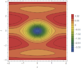
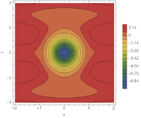
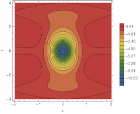
Figure 2: Time-dependent rational potentials $v_{2}^{(1)}(x,t)$, $v_{4}^{(1)}(x,t)$ and $v_{6}^{(1)}(x,t)$ with $E(t)=\sin t$.

We observe that all potentials $v_{n}^{(1)}$ with $n$ odd are singular at $x=0$, whereas those with $n$ even are regular for all values of $x$ and $t$. We depict some of these finite potentials in figure 2, noting that they possess well defined minima and finite asymptotic behaviour. The nontrivial solutions (7) to the TDSE for the Hamiltonians involving $v_{n}^{(1)}$ are

$$\phi_{n,m}^{(1)} = \mathcal{L}\left[\phi_{n}^{(0)}\right]\left(\phi_{m}^{(0)}\right),\qquad n\neq m$$ (56)

$$= i\sqrt{2}\frac{mH_{m-1}(iz)H_{n}(iz)-nH_{m}(iz)H_{n-1}(iz)}{\left(1+t^{2}\right)^{1/4}H_{n}(iz)}e^{i\kappa_{m}(t)}$$ (57)

and the nontrivial solutions obtained from (5) are

$$\hat{\phi}_{0}^{(1)} = e^{-z^{2}}\phi_{0}^{(0)},\quad\tilde{\phi}_{0}^{(1)}=\sqrt{2}F(z)\phi_{0}^{(0)},$$

$$\hat{\phi}_{1}^{(1)} = \frac{e^{-z^{2}}}{4z^{2}}\phi_{1}^{(0)},\quad\tilde{\phi}_{0}^{(1)}=\left[x\sqrt{1+t^{2}}-\sqrt{2}(1+t^{2})F(z)\right]\phi_{1}^{(0)},$$ (58)

$$\hat{\phi}_{2}^{(1)} = \frac{(1+t^{2})^{2}e^{-z^{2}}}{4(1+t^{2}+x^{2})^{2}}\phi_{2}^{(0)},\quad\tilde{\phi}_{2}^{(1)}=\frac{\left[x(x^{2}-t^{2}-1)\sqrt{1+t^{2}}-2\sqrt{2}(1+t^{2})^{2}F(z)\right]}{(1+t^{2}+x^{2})^{2}}\phi_{2}^{(0)},$$

where $F(z)$ denotes the Dawson integral $F(z):=\exp(-z^{2})\mathop{\displaystyle\int}\nolimits_{0}^{z}\exp(s^{2})ds$.

Finally we compute the non-Hermitian counterpart $H_{1}$ from the TDDE (8). Taking now $\eta_{1}$ to be of the same form as $\eta_{0}$ but different time-dependent parameters we make the Ansatz

$$\eta_{1}=e^{\gamma\left(t\right)x}e^{\delta\left(t\right)p}$$ (59)

and compute

$$H_{1}(x,p,t)=h_{1}(x+i\delta,p-i\gamma,t)-i\dot{\gamma}x-i\dot{\delta}p+\dot{\gamma}\delta.$$ (60)

Thus we obtain

$$H_{1,0} = p^{2}-2i\gamma p-\gamma^{2}+\alpha^{2}+E\beta-\frac{1}{1+t^{2}}-i\dot{\gamma}x+\dot{\gamma}\delta-i\dot{\delta}p$$ (61)

$$H_{1,1} = H_{1,0}+\frac{2}{(x+i\delta)^{2}},\quad H_{1,2}=H_{1,0}-\frac{4\left[1+t^{2}-(x+i\delta)^{2}\right]}{\left[1+t^{2}+(x+i\delta)^{2}\right]^{2}},$$ (62)

$$H_{1,3} = H_{1,0}+\frac{6\left[3\left(1+t^{2}\right)^{2}+(x+i\delta)^{4}\right]}{(x+i\delta)^{2}\left[3+3t^{2}+(x+i\delta)^{2}\right]^{2}},\ldots$$ (63)

By setting $\dot{\delta}=-2\gamma$ we may remove the linear term in $p$ and convert the Hamiltonian into a potential one. We notice that the singularities for $v_{1,n}$ with $n$ odd have been regularized in the non-Hermitian setting for $\delta\neq 0$. The remaining factors lead to further restrictions for $\delta$ when demanding regularity for the $H_{1,n}$. In this case we require in addition $|\delta|<1$ for $n=2$, $|\delta|<\sqrt{3}$ for $n=3$, $|\delta|>\sqrt{3+\sqrt{6}}$ for $n=4$,…

We verify that according to the commutative diagram (52) the intertwining operator relating $H_{0}$ and $H_{1}$ in (12) is indeed $L=\eta_{1}^{-1}\mathcal{L}\left[u\right]\eta_{0}$. From this we can now also compute the nontrivial solutions (14) to the TDSE

$$\psi_{1}(x,t)=e^{-\gamma x-i\gamma\delta}\hat{\phi}_{1}(x+i\delta),\qquad\text{and\qquad}\tilde{\psi}_{1}(x,t)=e^{-\gamma x-i\gamma\delta}\tilde{\phi}_{1}(x+i\delta).$$ (64)

Hence all of these systems are exactly solvable and the diagram (52) does indeed close. The two hierarchies of solvable time-dependent rational Hamiltonians are then directly computed from the expressions (23)-(31).

4.3 Solvable time-dependent Airy function potentials, two intertwinings

Finally we start again with a solution to the TDDE for $h_{0}$, $H_{0}$, $\eta_{0}$ and carry out the intertwining relations separately constructing $h_{1}$, $H_{1}$, but unlike as in section 4.1 we use the intertwining operator $L=\eta_{1}^{-1}\mathcal{L}\left[u\right]\eta_{0}$ involving an arbitrary operator $\eta_{1}$,

$$\begin{array}[]{ccccc}&H_{0}&~{}~{}\underrightarrow{\eta_{0}}{}{}&h_{0}&\\ L=\eta_{1}^{-1}\mathcal{L}\left[u\right]\eta_{0}&\downarrow&&\downarrow&\mathcal{L}\left[u\right]\\ &H_{1}&\underrightarrow{?}&h_{1}&\end{array}$$ (65)

which, by the closure of the diagram, must be the Dyson map for the system $1$.

We discuss this scenario for a somewhat less well known solution to the free particle TDSE in terms of Airy packet solutions as found forty years ago by Berry and Balazs [40], see also [41] for a different approach. The interesting feature of these wave packets is that they continually accelerate in a shape-preserving fashion despite the fact that no force is acting on them. Only more recently such type of waves have been realized experimentally in various forms, e.g. [42, 43, 44, 45, 46]. As in the previous section we modify the standard solution by a phase so that it solves the TDSE for $h_{GV}$

$$\phi_{0}^{X}\left(x,t\right)=\mathop{\mathrm{X}i}\left(\gamma x-\gamma^{4}t^{2}\right)\exp\left[i\gamma^{3}t\left(x-\frac{2\gamma^{3}t^{2}}{3}\right)-i\int\alpha^{2}+E\beta dt\right].$$ (66)

Here $\mathop{\mathrm{X}i}\left(z\right)$ denotes any of the two Airy functions $\mathop{\mathrm{A}i}\left(z\right)$ or $\mathop{\mathrm{B}i}\left(z\right)$ and $\gamma\in\mathbb{C}$ is a free parameter. Using once more the relation in (4), we obtain the intertwining operators and new Hamiltonians

$$\ell^{X} = \ell_{1}\left(t\right)\left[-i\gamma t^{3}-\gamma\frac{\mathop{\mathrm{X}i}^{\prime}\left(\gamma x-\gamma^{4}t^{2}\right)}{\mathop{\mathrm{X}i}\left(\gamma x-\gamma^{4}t^{2}\right)}+\partial_{x}\right],$$ (67)

$$h_{1}^{X} = 2\gamma^{3}(x-\gamma^{3}t^{2})-2\gamma^{2}\left[\frac{\mathop{\mathrm{X}i}^{\prime}\left(\gamma x-\gamma^{4}t^{2}\right)}{\mathop{\mathrm{X}i}\left(\gamma x-\gamma^{4}t^{2}\right)}\right]^{2}+\alpha^{2}+E\beta+i\frac{\left(\ell_{1}\right)_{t}}{\ell_{1}},$$

with $\mathop{\mathrm{X}i}^{\prime}\left(z\right)$ denoting the derivative of the Airy functions. Taking $\ell_{1}$ to be a constant and $\gamma\in\mathbb{R}$ these are indeed Hermitian Hamiltonians. We also note that $h_{1}^{X}$ becomes singular when $\gamma x-\gamma^{4}t^{2}$ equals a zero of the Airy functions on the negative real axis. In addition, $h_{1}^{B}$ becomes singular when $\pi/3<\arg(\gamma x-\gamma^{4}t^{2})<\pi/2$. The nontrivial solutions according to (7) are computed to

$$\phi_{1}^{A/B}=\ell^{A/B}(\phi_{0}^{B/A})=\pm\frac{\ell_{1}(t)\gamma\exp\left[-\frac{1}{3}i\left(2\gamma^{6}t^{3}-3\gamma^{3}tx+3\int^{t}\left[\alpha(s)^{2}+\beta(s)\kappa(s)\right]\,ds\right)\right]}{\pi\mathop{\mathrm{A}i}/\mathop{\mathrm{B}i}\left(\gamma x-\gamma^{4}t^{2}\right)}.$$ (68)

We have constructed these solutions from the two linearly independent solutions to the original TDSE rather than from one particular solution with different parameters $\gamma$, i.e.

$$\phi_{1}^{A/B}(\gamma_{1},\gamma_{2})=\mathcal{L}[\phi_{0}^{A/B}(\gamma_{1})](\phi_{0}^{A/B}(\gamma_{2}))$$ (69)

are also solutions. Additional solutions can also be obtained in a straightforward manner from (5).

For fixed values of time we observe in figure 3 panel (a) the two characteristic qualitatively different types of behaviour of the Airy wave function, that is being oscillatory up to a certain point $x=x_{0}$ and beyond which the density distribution becomes decaying. We observe further that for increasing positive time, or decreasing negative time, the wave packets accelerate. For the density wave function of the partner Hamiltonian in panel (b) we observe this behaviour for one dominating value of $\gamma$ modulated by the other.

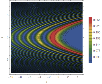
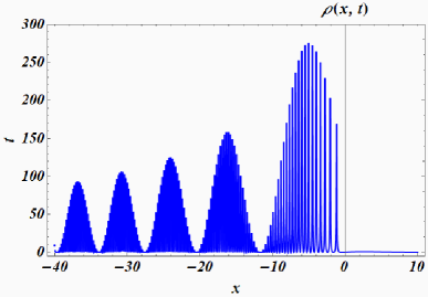
Figure 3: Probability densities for Airy wavepackets for solutions of the level 1 and 2 TDSE $\rho_{0}=\left|\phi_{0}^{A}(\gamma=0.75)\right|^{2}$ and $\rho_{1}=\left|\phi_{1}^{A}(t=1,\gamma_{1}=0.2,\gamma_{2}=2.0)\right|^{2}$, left and right panel, respectively.

According to our commutative diagram (65) we calculate next the non-Hermitian counterpart $H_{1}^{X}$ using the intertwining operator $L=\eta_{1}^{-1}\mathcal{L}\left[\phi_{0}^{X}\right]\eta_{0}$ with $\eta_{1}$ as specified in (59). We obtain

$$H_{1}^{X}(x,p,t)=h_{1}^{X}(x+i\delta,p-i\gamma,t)-i\dot{\gamma}x-i\dot{\delta}p+\dot{\gamma}\delta.$$ (70)

We verify the closure of the diagram by noting that $H_{1}^{X}$ satisfies indeed the TDDE with $h_{1}^{X}$, $\eta_{1}$.

The above mentioned singularities on the real axis are now regularized.

5 Reduced Swanson model hierarchy

Next we consider a model that is build from a slightly more involved time-dependent Dyson map. We proceed as outlined in the commutative diagram (52). Our simple starting point is a non-Hermitian, but $\mathcal{PT}$-symmetric, Hamiltonian that may be viewed as reduced version of the well-studied Swanson model [47]

$$H_{0}=H_{RS}=ig\left(t\right)xp.$$ (71)

We follow the same procedure as before and solve at first the TDDE for $\eta_{0}$ and $h_{0}$ with given $H_{0}$. In this case the arguments in the exponentials of the time-dependent Dyson map can no longer be linear and we therefore make the Ansatz

$$\eta_{0}=e^{\lambda\left(t\right)xp}e^{\zeta\left(t\right)p^{2}/2}.$$ (72)

The right hand side of the TDDE (8) is then computed to

$$h_{0}=h_{RS}=\left[\left(g\zeta+i\frac{\dot{\zeta}}{2}\right)\cos(2\lambda)+\left(ig\zeta-\frac{\dot{\zeta}}{2}\right)\sin(2\lambda)\right]p^{2}+i(g+\dot{\lambda})xp.$$ (73)

Thus for $h_{0}$ to be Hermitian we have to impose

$$\dot{\lambda}=-g,\quad\dot{\zeta}=-2g\zeta\tan 2\lambda,$$ (74)

so that we obtain a free particle Hamiltonian with a time-dependent mass $m(t)$

$$h_{0}=h_{RS}=\frac{1}{2m(t)}p^{2},\qquad\text{with }m(t)=\frac{1}{2g\zeta\sec(2\lambda)}.$$ (75)

Time-dependent masses have been proposed as a possible mechanism to explain anomalous nuclear reactions which can not been explained by existing conventional theories in nuclear physics, see e.g. [48]. The reality constraints (74) can be solved by

$$\lambda(t)=-\int^{t}g\left(s\right)ds,\quad\text{and \quad}\zeta(t)=c\sec\left(2\int^{t}g\left(s\right)ds\right),\quad$$ (76)

with constant $c$. Thus the time-dependent mass $m(t)$ can be expressed entirely in terms of the time-dependent coupling $g(t)$. An exact solution to the TDSE for $h_{RS}$ can be found for instance in [49] when setting in there the time-dependent frequency to zero

$$\phi_{n}^{(0)}\left(x,t\right) = \frac{e^{i\alpha_{0,n}(t)}}{\pi^{1/4}\sqrt{n!2^{n}\varrho(t)}}\exp\left[m(t)\left(i\frac{\dot{\varrho}(t)}{\varrho(t)}-\frac{1}{m(t)\varrho^{2}(t)}\right)\frac{x^{2}}{2}\right]H_{n}\left[\frac{x}{\varrho(t)}\right],$$ (77)

$$\alpha_{0,n}(t) = ~{}\ -\mathop{\displaystyle\int}\nolimits_{0}^{t}\frac{\left(n+1/2\right)}{m(s)\varrho^{2}(s)}ds.$$ (78)

For (77) to be a solution, the auxiliary function $\varrho(t)$ needs to obey the dissipative Ermakov-Pinney equation with vanishing linear term

$$\ddot{\varrho}+\frac{\dot{m}}{m}\dot{\varrho}=\frac{1}{m^{2}\varrho^{3}}.$$ (79)

We derive an explicit solution for this equation in appendix A. Evaluating the formulae in (4), with $h_{0}$ and $h_{1}$ divided by $2m(t)$, we obtain the intertwining operators and the partner Hamiltonians

$$\ell_{n}^{(1)} = \ell_{1}\left(t\right)\left[\frac{x}{\varrho^{2}}-\frac{2nH_{n-1}\left[x/\varrho\right]}{\varrho H_{n}\left[x/\varrho\right]}-ixm\frac{\dot{\varrho}}{\varrho}+\partial_{x}\right],$$ (80)

$$h_{1,n} = h_{0}+\frac{4n}{m\varrho^{2}}\left[\frac{nH_{n-1}^{2}\left[x/\varrho\right]-(n-1)H_{n-2}\left[x/\varrho\right]H_{n}\left[x/\varrho\right]}{H_{n}^{2}\left[x/\varrho\right]}\right]+\frac{1}{m\varrho^{2}}+i\left[\frac{\dot{\ell}_{1}}{\ell_{1}}-\frac{\dot{\varrho}}{\varrho}\right],~{}~{}~{}$$

respectively. As in the previous section, the imaginary part of the Hamiltonian only depends on time and can be made to vanish with the suitable choice of $\ell_{1}=\varrho$. For concrete values of $n$ we obtain for instance the time-dependent Hermitian Hamiltonians

$$h_{1,0} = \frac{p^{2}}{2m}+\frac{1}{m\varrho^{2}},\qquad h_{1,1}=h_{1,0}+\frac{1}{mx^{2}},\qquad h_{1,2}=h_{1,0}+\frac{4(\varrho^{2}+2x^{2})}{m(\varrho^{2}-2x^{2})^{2}},$$ (81)

$$h_{1,3} = h_{1,0}+\frac{3(3\varrho^{4}+4x^{4})}{m(2x^{3}-3x\varrho^{2})^{2}},\qquad h_{1,4}^{(4)}=h_{1,0}+\frac{8\left(9\varrho^{6}-12x^{4}\varrho^{2}+18x^{2}\varrho^{4}+8x^{6}\right)}{m\left(3\varrho^{4}-12x^{2}\varrho^{2}+4x^{4}\right)^{2}}.~{}~{}~{}~{}~{}~{}$$ (82)

Notice that all these Hamiltonians are singular at certain values of $x$ and $t$ as $\varrho$ is real. Solutions to the TDSE for the Hamiltonian $h_{1,n}$ can be computed according to (7)

$$\phi_{n,k}^{(1)}\left(x,t\right)=\ell_{n}^{(1)}(\phi_{k}^{(0)})=\frac{2^{3/2}}{\sqrt{k-n}}\left[\frac{kH_{k-1}\left[x/\varrho\right]}{H_{k}\left[x/\varrho\right]}-\frac{nH_{n-1}\left[x/\varrho\right]}{H_{n}\left[x/\varrho\right]}\right]\phi_{k}^{(0)},~{}~{}\ n\neq k.$$ (83)

Both $\phi_{n}^{(0)}$ and $\phi_{n,k}^{(1)}$ are square integrable functions with $L^{2}(\mathbb{R})$-norm equal to $1$. In figure 4 we present the computation for some typical probability densities obtained from these functions. Notice that demanding $m(t)>0$ we need to impose some restrictions for certain choices of $g(t)$.

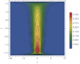
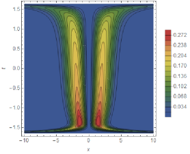
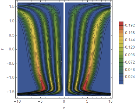
Figure 4: Probability densities $\left|\phi_{0}^{(0)}\right|^{2}$, $\left|\phi_{1}^{(0)}\right|^{2}$, $\left|\phi_{1,7}^{(1)}\right|^{2}$ from left to right for $g(t)=(1+t^{2})/4$, $m(t)=\left[1+\cos(t+t^{3}/3)\right]/(1+t^{2})$, $\varrho(t)=\sqrt{1+[C+B\tan(t/2+t^{3}/6)]^{2}}$ with $B=1/2$ and $C=1$.

Next we compute the non-Hermitian counterpart $H_{1\text{ }}$with a concrete choice for the second Dyson map. Taking $\eta_{1}$ for instance to be of the same form as in (59) the non-Hermitian Hamiltonian is formally the same as in equation (60). In our concrete case we obtain for instance

$$H_{1,1}=\frac{p^{2}}{2m}+\frac{1}{m(x+i\delta)^{2}}-i\dot{\gamma}x+\frac{1}{m\varrho^{2}}-\frac{\gamma^{2}}{2m}+\dot{\gamma}\delta,$$ (84)

where we have also imposed the constraint $\dot{\delta}=-\gamma/m$ to eliminate a linear term in $p$, hence making the Hamiltonian a potential one. The solutions for the TDSEs for $H_{0}$ and $H_{1,n}$ are

$$\psi_{n}^{(0)}=\eta_{0}^{-1}\phi_{n}^{(0)},\quad\text{and\quad}\psi_{n,k}^{(1)}=\eta_{1}^{-1}\phi_{n,k}^{(1)},$$ (85)

respectively.

5.1 Lewis-Riesenfeld invariants

Having solved the TDDE for $\eta_{0}$ and $\eta_{1}$ we can now also verify the various intertwining relations for the Lewis-Riesenfeld invariants as derived in section 3. We proceed here as depicted in the following commutative diagram

$$\begin{array}[]{ccccc}&I_{0}^{h}&~{}~{}\underrightarrow{\eta_{0}}{}{}&I_{0}^{H}&\\ \mathcal{L}\left[\check{\phi}\right]&\downarrow&&\downarrow&?\\ &I_{1}^{h}&\underrightarrow{\eta_{1}}&I_{1}^{H}&\end{array}$$ (86)

See also the more general schematic representation in figure 1. We start with the Hermitian invariant $I_{0}^{h}$ from which we compute the non-Hermitian invariant $I_{0}^{H}$ using the Dyson map $\eta_{0}$ as specified in (72). Subsequently we use the intertwining operator $\ell_{n}^{(1)}$ in (80) to compute the Hermitian invariants $I_{1,n}^{h}$ for the Hamiltonians $h_{1,n}$. The invariant $I_{1}^{H}$ is then computed from the adjoint action of $\eta_{1}^{-1}$ as specified in (59). Finally, the intertwining relation between the non-Hermitian invariants $I_{0}^{H}$ and $I_{1}^{H}$ is just given by the closure of the diagram in (86).

The invariant for the Hermitian Hamiltonian $h_{0}$ has been computed previously in [49]

$$I_{0}^{h}=A_{h}(t)p^{2}+B_{h}(t)x^{2}+C_{h}(t)\{x,p\},$$ (87)

where the time-dependent coefficients are

$$A_{h}=\frac{\varrho^{2}}{2},\quad B_{h}=\frac{1}{2}\left(\frac{1}{\varrho^{2}}+m^{2}\dot{\varrho}^{2}\right),\quad C_{h}=-\frac{1}{2}m\varrho\dot{\varrho}.$$ (88)

It then follows from

$$\left[I_{0}^{h},h_{0}\right]=\frac{2i}{m}\left(C_{h}p^{2}+\frac{1}{2}B_{h}\{x,p\}\right),\quad\dot{A}_{h}=-\frac{2}{m}C_{h},\quad\dot{B}_{h}=0,\quad\dot{C}_{h}=-\frac{1}{m}B_{h},$$ (89)

that the defining relation (32) for the invariant is satisfied by $I_{0}^{h}$. According to the relation (35), the non-Hermitian invariant $I_{0}^{H}$ for the non-Hermitian Hamiltonian $H_{0}$ is simply computed by the adjoint action of $\eta_{0}^{-1}$ on $I_{0}^{h}$. Using the expression (72) we obtain

$$I_{0}^{H}=\eta_{0}^{-1}I_{0}^{h}\eta_{0}=A_{H}(t)p^{2}+B_{H}(t)x^{2}+C_{H}(t)\{x,p\},$$ (90)

with

$$A_{H}=\frac{1}{2}e^{-2i\lambda}\rho^{2}-\zeta^{2}B_{H}-i\zeta m\rho\dot{\rho},\quad B_{H}=\frac{e^{2i\lambda}\left(1+m^{2}\rho^{2}\dot{\rho}^{2}\right)}{2\rho^{2}},\quad C_{H}=i\zeta B_{H}-\frac{1}{2}m\rho\dot{\rho}.$$ (91)

We verify that $I_{0}^{H}$ is indeed an invariant for $H_{0}$ according to the defining relation (32), by computing

$$\left[I_{0}^{H},H_{0}\right]=2g\left(A_{H}p^{2}-B_{H}x^{2}\right),\quad\dot{A}_{H}=2igA_{H},\quad\dot{B}_{h}=-2igB_{H},\quad\dot{C}_{H}=0,$$ (92)

using the constraints (74) and (79).

Given the intertwining operators $\ell_{n}^{(1)}$ in (80) and the invariant $I_{0}^{h}$, we can use the intertwining relation (36) to compute the invariants $I_{1,n}^{h}$ for the Hamiltonians $h_{1,n}$ in (5). Solving (36) we find

$$I_{1,n}^{h}=I_{0}^{h}+1+4n^{2}\frac{H_{n-1}^{2}\left[x/\varrho\right]^{2}}{H_{n}^{2}\left[x/\varrho\right]^{2}}-4n(n-1)\frac{H_{n-2}\left[x/\varrho\right]}{H_{n}^{2}\left[x/\varrho\right]}.$$ (93)

We verify that this expression solves (32). The last invariant in our quadruple is

$$I_{1,n}^{H}(x,p)=\eta_{1}^{-1}I_{1,n}^{h}(x,p)\eta_{1}=I_{1,n}^{h}(x+i\delta,p-i\gamma)$$ (94)

Finally we may also verify the eigenvalue equations for the four invariants. Usually this is of course the first consideration as the whole purpose of employing Lewis-Riesenfeld invariants is to reduce the TDSE to the much easier to solve eigenvalue equations. Here this computation is simply a consistency check. With

$$\check{\phi}_{n}^{(0)} = e^{-i\alpha_{0,n}}\phi_{n}^{(0)},\quad\check{\phi}_{n,m}^{(1)}=e^{-i\alpha_{0,m}}\phi_{n,m}^{(1)},\quad$$ (95)

$$\check{\psi}_{n}^{(0)} = e^{-i\alpha_{0,n}}\psi_{n}^{(0)},\quad\check{\psi}_{n,m}^{(1)}=e^{-i\alpha_{0,m}}\psi_{n,m}^{(1)},$$ (96)

and $\alpha_{0,n}$ as specified in equation (78) we compute

$$I_{0}^{h}\check{\phi}_{n}^{(0)} = \left(n+1/2\right)\check{\phi}_{n}^{(0)},~{}~{}~{}\ \ \ I_{1,n}^{h}\check{\phi}_{n,m}^{(1)}=\left(m+1/2\right)\check{\phi}_{n,m}^{(1)},~{}~{}$$ (97)

$$I_{0}^{H}~{}\check{\psi}_{n}^{(0)} = \left(n+1/2\right)\check{\psi}_{n}^{(0)},~{}~{}~{}\ \ \ I_{1,n}^{H}\check{\psi}_{n,m}^{(1)}=\left(m+1/2\right)\check{\psi}_{n,m}^{(1)}.$$ (98)

As expected all eigenvalues are time-independent.

6 Conclusions

We have generalized the scheme of time-dependent Darboux transformations to allow for the treatment of non-Hermitian Hamiltonians that are $\mathcal{PT}$-symmetric/quasi-Hermitian. It was essential to employ intertwining operators different from those used in the Hermitian scheme previously proposed. We have demonstrated that the quadruple of Hamiltonians, two Hermitian and two non-Hermitian ones, can be constructed in alternative ways, either by solving two TDDEs and one intertwining relation or by solving one TDDE and two intertwining relations. For a special class of Dyson maps it is possible to independently carry out the intertwining relations for the Hermitian and non-Hermitian sector, which, however, forced the seed function used in the construction of the intertwining operator to obey certain constraints. We extended the scheme to the construction of the entire time-dependent Darboux-Crum hierarchies. We also showed that the scheme is consistently adaptable to construct Lewis-Riesenfeld invariants by means of intertwining relations. Here we verified this for a concrete system by having already solved the TDSE, however, evidently it should also be possible to solve the eigenvalue equations for the invariants first and subsequently construct the solutions to the TDSE. As in the Hermitian case, our scheme allows to treat time-dependent systems directly instead of having to solve the time-independent system first and then introducing time by other means. The latter is not possible in the context of the Schrödinger equation, unlike as in the context of nonlinear differential equations that admit soliton solutions, where a time-dependence can be introduced by separate arguments, such as for instance using Galilean invariance. Naturally it will be very interesting to apply our scheme to the construction of multi-soliton solutions.

Appendix A Appendix

We briefly explain how to solve the Ermakov-Pinney equation with dissipative term (79)

$$\ddot{\varrho}+\frac{\dot{m}}{m}\dot{\varrho}=\frac{1}{m^{2}\varrho^{3}}.$$ (99)

The solutions to the standard version of the equation [50, 51]

$$\ddot{\sigma}+\lambda(t)\sigma=\frac{1}{\sigma^{3}}$$ (100)

are well known to be of the form [51]

$$\sigma(t)=\left(Au^{2}+Bv^{2}+2Cuv\right)^{1/2},$$ (101)

with $u(t)$ and $v(t)$ denoting the two fundamental solutions to the equation $\ddot{\sigma}+\lambda(t)\sigma=0$ and $A$, $B$, $C$ are constants constrained as $C^{2}=AB-W^{-2}$ with Wronskian $W=u\dot{v}-v\dot{u}$. The solutions to the equation with an added dissipative term proportional to $\dot{\sigma}$ are not known in general. However, the equation of interest here, (99), which has the linear term removed may be solved exactly. For this purpose we assume $\varrho(t)$ to be of the form

$$\varrho(t)=f[q(t)],\qquad\ \ \ \text{with }q(t)=\mathop{\displaystyle\int}\nolimits^{t}\frac{1}{m(s)}ds.$$ (102)

Using this form, equation (99) transforms into

$$\frac{d^{2}f}{dq^{2}}=\frac{1}{f^{3}},$$ (103)

which corresponds to (100) with $\lambda(t)=0$. Taking the linear independent solutions to that equation to be $u(t)=1$ and $v(t)=q$, we obtain

$$f(q)=\frac{\pm 1}{\sqrt{B}}\sqrt{1+(Bq+C)^{2}}$$ (104)

and hence with (102) a solution to (99).

Acknowledgments: JC and TF are supported by City, University of London Research Fellowships.

References

- [1] G. Darboux, On a proposition relative to linear equations, physics/9908003, Comptes Rendus Acad. Sci. Paris 94, 1456–59 (1882).
- [2] E. Witten, Dynamical breaking of supersymmetry, Nucl. Phys. B188, 513 (1981).
- [3] F. Cooper, A. Khare, and U. Sukhatme, Supersymmetry and quantum mechanics, Phys. Rept. 251, 267–385 (1995).
- [4] V. G. Bagrov and B. F. Samsonov, Darboux transformation of the Schrödinger equation, Physics of Particles and Nuclei 28(4), 474 (1997).
- [5] S. Longhi and G. Della Valle, Invisible defects in complex crystals, Annals of Physics 334, 35–46 (2013).
- [6] F. Correa, V. Jakubskỳ, and M. S. Plyushchay, PT-symmetric invisible defects and confluent Darboux-Crum transformations, Physical Review A 92(2), 023839 (2015).
- [7] V. B. Matveev and M. A. Salle, Darboux transformation and solitons, (Springer, Berlin) (1991).
- [8] F. Correa and M. S. Plyushchay, Hidden supersymmetry in quantum bosonic systems, Annals of Physics 322(10), 2493–2500 (2007).
- [9] J. Cen, F. Correa, and A. Fring, Degenerate multi-solitons in the sine-Gordon equation, J. Phys. A: Math. Theor. 50, 435201 (2017).
- [10] J. M. Guilarte and M. S. Plyushchay, Perfectly invisible PT-symmetric zero-gap systems, conformal field theoretical kinks, and exotic nonlinear supersymmetry, J. of High Energy Phys. 2017(12), 61 (2017).
- [11] J. Cen and A. Fring, Asymptotic and scattering behaviour for degenerate multi-solitons in the Hirota equation, arXiv preprint arXiv:1804.02013 (2018).
- [12] V. G. Bagrov and B. F. Samsonov, Supersymmetry of a nonstationary Schrödinger equation, Physics Letters A 210(1-2), 60–64 (1996).
- [13] D.-Y. Song and J. R. Klauder, Generalization of the Darboux transformation and generalized harmonic oscillators, J. of Phys. A: Math. and Gen. 36(32), 8673 (2003).
- [14] A. A. Suzko and A. Schulze-Halberg, Darboux transformations and supersymmetry for the generalized Schrödinger equations in (1+ 1) dimensions, J. of Phys. A: Math. and Theor. 42(29), 295203 (2009).
- [15] F. G. Scholtz, H. B. Geyer, and F. Hahne, Quasi-Hermitian Operators in Quantum Mechanics and the Variational Principle, Ann. Phys. 213, 74–101 (1992).
- [16] C. M. Bender, Making sense of non-Hermitian Hamiltonians, Rept. Prog. Phys. 70, 947–1018 (2007).
- [17] A. Mostafazadeh, Pseudo-Hermitian Representation of Quantum Mechanics, Int. J. Geom. Meth. Mod. Phys. 7, 1191–1306 (2010).
- [18] C. Figueira de Morisson Faria and A. Fring, Time evolution of non-Hermitian Hamiltonian systems, J. Phys. A39, 9269–9289 (2006).
- [19] A. Mostafazadeh, Time-dependent pseudo-Hermitian Hamiltonians defining a unitary quantum system and uniqueness of the metric operator, Physics Letters B 650(2), 208–212 (2007).
- [20] M. Znojil, Time-dependent version of crypto-Hermitian quantum theory, Physical Review D 78(8), 085003 (2008).
- [21] J. Gong and Q.-H. Wang, Time-dependent PT-symmetric quantum mechanics, J. Phys. A: Math. and Theor. 46(48), 485302 (2013).
- [22] A. Fring and M. H. Y. Moussa, Unitary quantum evolution for time-dependent quasi-Hermitian systems with nonobservable Hamiltonians, Physical Review A 93(4), 042114 (2016).
- [23] A. Fring and T. Frith, Exact analytical solutions for time-dependent Hermitian Hamiltonian systems from static unobservable non-Hermitian Hamiltonians, Phys. Rev. A 95, 010102(R) (2017).
- [24] A. Fring and T. Frith, Metric versus observable operator representation, higher spin models, Eur. Phys. J. Plus, 133: 57 (2018).
- [25] A. Fring and T. Frith, Mending the broken PT-regime via an explicit time-dependent Dyson map, Phys. Lett. A, 2318 (2017).
- [26] A. Fring and T. Frith, Solvable two-dimensional time-dependent non-Hermitian quantum systems with infinite dimensional Hilbert space in the broken PT-regime, J. of Phys. A: Math. and Theor. 51(26), 265301 (2018).
- [27] A. Mostafazadeh, Energy Observable for a Quantum System with a Dynamical Hilbert Space and a Global Geometric Extension of Quantum Theory, arXiv preprint arXiv:1803.04175 (2018).
- [28] A. Fring and T. Frith, Quasi-exactly solvable quantum systems with explicitly time-dependent Hamiltonians, preprint arXiv:1808.03547, Phys. Lett. A (2018) https://doi.org/10.1016/j.physleta.2018.10.043.
- [29] M. M. Crum, Associated Sturm-Liouville systems, The Quarterly Journal of Mathematics 6(1), 121–127 (1955).
- [30] I. Gelfand, S. Gelfand, V. Retakh, and R. L. Wilson, Quasideterminants, Adv. Math 193(1), 56–141 (2005).
- [31] F. Correa and A. Fring, Regularized degenerate multi-solitons, Journal of High Energy Physics 2016(9), 8 (2016).
- [32] J. Cen, F. Correa, and A. Fring, Integrable nonlocal Hirota equations, arXiv:1710.11560 (2017).
- [33] M. Maamache, O. K. Djeghiour, N. Mana, and W. Koussa, Pseudo-invariants theory and real phases for systems with non-Hermitian time-dependent Hamiltonians, The European Physical Journal Plus 132(9), 383 (2017).
- [34] H. Lewis and W. Riesenfeld, An Exact quantum theory of the time dependent harmonic oscillator and of a charged particle time dependent electromagnetic field, J. Math. Phys. 10, 1458–1473 (1969).
- [35] W. Gordon, Der Comptoneffekt nach der Schrödinger Theorie, Zeit. für Physik 40, 117–133 (1926).
- [36] D. M. Volkov, On a class of solutions of the Dirac equation, Zeit. für Physik 94, 250 (1935).
- [37] C. Figueira de Morisson Faria, A. Fring, and R. Schrader, Analytical treatment of stabilization, Laser Physics 9, 379–387 (1999).
- [38] W. Liu, D. N. Neshev, I. V. Shadrivov, A. E. Miroshnichenko, and Y. S. Kivshar, Plasmonic Airy beam manipulation in linear optical potentials, Optics Letters 36(7), 1164–1166 (2011).
- [39] W. Miller Jr, Symmetry and separation of variables, (1977).
- [40] M. V. Berry and N. L. Balazs, Nonspreading wave packets, Am. J. of Phys. 47(3), 264–267 (1979).
- [41] F. Gori, M. Santarsiero, R. Borghi, and G. Guattari, The general wavefunction for a particle under uniform force, Euro. J. of Phys. 20(6), 477 (1999).
- [42] G. A. Siviloglou, J. Broky, A. Dogariu, and D. N. Christodoulides, Observation of accelerating Airy beams, Phys. Rev. Lett. 99(21), 213901 (2007).
- [43] G. A. Siviloglou and D. N. Christodoulides, Accelerating finite energy Airy beams, Optics Lett. 32(8), 979–981 (2007).
- [44] J. Baumgartl, M. Mazilu, and K. Dholakia, Optically mediated particle clearing using Airy wavepackets, Nature photonics 2(11), 675 (2008).
- [45] T. Vettenburg, H. I. C. Dalgarno, J. Nylk, C. Coll-Lladó, D. E. K. Ferrier, T. Čižmár, F. J. Gunn-Moore, and K. Dholakia, Light-sheet microscopy using an Airy beam, Nature methods 11(5), 541 (2014).
- [46] A. Patsyk, M. A. Bandres, R. Bekenstein, and M. Segev, Observation of Accelerating Wave Packets in Curved Space, Phys. Rev. X 8(1), 011001 (2018).
- [47] M. S. Swanson, Transition elements for a non-Hermitian quadratic Hamiltonian, J. Math. Phys. 45, 585–601 (2004).
- [48] M. Davidson, Variable mass theories in relativistic quantum mechanics as an explanation for anomalous low energy nuclear phenomena, in J. of Phys.: Conference Series, volume 615, page 012016, IOP Publishing, 2015.
- [49] I. A. Pedrosa, Exact wave functions of a harmonic oscillator with time-dependent mass and frequency, Phys. Rev. A 55(4), 3219 (1997).
- [50] V. Ermakov, Transformation of differential equations,, Univ. Izv. Kiev. 20, 1–19 (1880).
- [51] E. Pinney, The nonlinear differential equation , Proc. Amer. Math. Soc. 1, 681(1) (1950).