The k-core as a predictor of structural collapse in mutualistic ecosystems

Abstract

Abstract

Collapses of dynamical systems into irrecoverable states are observed in ecosystems, human societies, financial systems and network infrastructures. Despite their widespread occurrence and impact, these events remain largely unpredictable. In searching for the causes for collapse and instability, theoretical investigations have been so far unable to determine quantitatively the influence of the structural features of the network formed by the interacting species. Here, we derive the condition for the stability of a mutualistic ecosystem as a constraint on the strength of the dynamical interactions between species and a topological invariant of the network: the k-core. Our solution predicts that when species located at the maximum k-core of the network go extinct as a consequence of sufficiently weak interaction strengths the system will reach the tipping point of its collapse. As a key variable involved in collapse phenomena, monitoring the k-core of the network may prove a powerful method to anticipate catastrophic events in the vast context that stretches from ecological and biological networks to finance.

I Introduction

A complex dynamical system collapses when a small perturbation in the parameters characterizing the species interactions causes a large-scale extinction of the species in the system may3 ; strogatz ; caldarelli ; shlomo ; sheffer1 ; sheffer2 ; allesina ; gao ; bascompte-linear ; coyte ; may-banking ; guido-banking . The tipping point at which the system suddenly shifts to the irrecoverable state is, for practical purposes, the most important quantity one wishes to know sheffer1 ; sheffer2 ; gore . It is a function of the dynamical and structural parameters of the system determined by the fixed point solution of the nonlinear equations describing the system’s dynamics may3 . However, the tipping point is hard to determine, due to the difficulties encountered in solving the nonlinear dynamical equations to quantify the dependence of the fixed point solution on the system parameters and, in particular, on the features of the underlying network of interacting species in the system may3 ; caldarelli ; gao ; sheffer2 . Indeed, no exact analytical result exists, so far, that relates the network properties to the fixed points of the dynamical system. Here, we first study numerically the fixed point equations of a dynamical system of mutualistic species and then derive the analytical solution to compute the tipping point using a logic approximation. Our solution reveals that the root cause of the system collapse is the extinction of species located in the maximum k-core of the network.

The concept of k-core was introduced in social sciences  seidman to define network cohesion and was then applied in many other contexts wormald , including the robustness of random networks dorogotsev , the structure of the internet carmi ; hamelin , viral spreading in social networks gallos , the large-scale structure of brain networks sporn , and the jamming transition kate . For a network of interacting species, the k-core is the portion of the network that remains after iteratively removing from the network all species linked to fewer than $k$ other species (see Figs. 1a, b and Supplementary Information Section  I  seidman ; dorogotsev ). For a given $k$, the subset of species in the k-core consists of the periphery, called the k-shell, and the remaining k+1-core; therefore, the k-shell is the region of the k-core not included in the k+1-core (Fig. 1a). Thus, the network has a nested structure of k-cores with increasing k-shells of order $k_{s}$, starting from the periphery of the network or 1-shell, $k_{s}=1,$ and its 1-core which includes all the network (except for isolated nodes). The 1-core contains the 2-core, and so on, up to the innermost core of the network which is the maximum k-core labeled by the “k-core number” $k^{\rm max}_{\rm core}$. The k-core number is a topological invariant of the network dorogotsev .

II Model of a mutualistic ecosystem

We consider complex systems populated by $N$ interacting species, also referred to as network nodes, whose directed interactions can be graphically portrayed as links in a network via the adjacency matrix $A_{ij}$ such that $A_{ij}=1$ if species $i$ interact with $j$, and $A_{ij}=0$ otherwise. In general $A_{ij}\neq A_{ji}$ for directed networks. The strength of the directed interaction from species $i$ to $j$ is $\gamma_{ij}$. In this paper we consider the case of mutualistic ecosystems where organisms of different species cooperate with each other by benefiting from the activities of the other, such as plants and pollinators. These systems are characterized by positive interactions between the species, $\gamma_{ij}>0$. Dynamical systems with positive and negative interactions, such as neuron, genes or predator-prey ecosystems, are out of the scope of the present work and will be treated in a follow-up.

The state of the system is encoded in the multiplet of species densities $\vec{x}(t)\equiv(x_{1}(t),\dots,x_{N}(t))$ evolving in time towards a fixed point $\vec{x}^{*}$, where $\dot{\vec{x}}^{*}=\vec{0}$  strogatz . When the species do not interact, i.e. for $\gamma_{ij}=0$, each species density changes through time as $\dot{x}_{i}(t)=f_{i}(x_{i})$, and the fixed points are found by solving $f_{i}(x_{i}^{*})=0$ for all $i$. When the species interact according to $\gamma_{ij}$, $x_{i}(t)$ is influenced by the densities $x_{j}(t)$ of the species linked to it in the network of interactions. While these interactions are generally complex, it is generally recognized that they saturate when the density of interacting species increases may ; holland ; alon ; amit ; thebault ; bastolla . This occurs in mutualistic interactions between species in ecosystems, for which the benefit accorded by one species to another saturates to a limiting value may ; holland ; thebault ; bastolla . In biology, the expression level of gene products are modeled by Hill or sigmoidal response functions which saturate at high concentrations of the interacting gene (SI Section II)  alon . Enzymatic reactions are also modeled by Hill functions in the Michaelis-Menten equation  alon and firing rates of neurons saturate at high membrane potential via sigmoidal functions amit ; sompolinsky .

In the following, we treat explicitly the paradigmatic case of dynamical systems of ecological mutualistic networks, but the results we obtain hold true for the larger class of nonlinear systems where a Hill or sigmoidal function models the interactions. A network of mutualistic species describes a system of symbionts obligated to each other because they cannot survive independently thebault ; holland ; may , e.g., an ecosystem of plants and pollinators (Fig. 1b). The dynamics of species densities, $x_{i}(t)$, interacting via the network $A_{ij}$ with directed and positive interaction strengths $\gamma_{ij}$, is described by the following set of nonlinear differential equations holland ; thebault ; may ; bastolla ; holland3 :

$$\dot{x_{i}}(t)\ =\ -dx_{i}-sx_{i}^{2}+\sum_{j=1}^{N}A_{ij}\gamma_{ij}\frac{x_{i}x_{j}}{\alpha+\sum_{k=1}^{N}A_{ik}x_{k}}\ ,\,\,i\in\{1,\cdot\cdot\cdot,N\}\ .$$ (1)

Here $d>0$ is the death rate of the species, $s>0$ is the self-limitation parameter modelling the intraspecific competition that limits a species’ growth once $x_{i}$ exceeds a certain value, $\alpha$ is the half-saturation constant, and $\gamma_{ij}>0$ is the mutualistic interaction strength between species $i$ and $j$ characterizing the strength of the nonlinear interaction term. The dynamical parameters $(\{\gamma_{ij}\},d,s,\alpha)$ have been extensively discussed in the literature  holland ; thebault ; may ; bastolla ; holland3 . The network is bipartite between, e.g., plants and pollinators (Fig. 1b). Our goal is to bridge the gap from structure to dynamics by obtaining the fixed point solution of dynamical equations to predict the tipping point of collapse in terms of a feature of the network.

III Numerical analysis of the ecosystem collapse

We start by performing a numerical study of the tipping point of the system (details in Methods Section and in SI Section III), and then we elaborate our analytical solution based on approximations supported by the numerical evidence. Figures 2b-f show the numerical solution of the Eqs. (1) for different parameters on a real plant-pollinator mutualistic network from the Chilean Andes obtained from Ref. arroyo (Net #10 in Supplementary Table 1). We plot the fixed point average density (properly rescaled) $\langle x^{*}\rangle=N^{-1}\sum_{i}x_{i}^{*}$ as a function of $K_{\gamma}=\frac{\alpha s(\gamma+d)}{(\gamma-d)^{2}}$, which is the main control parameter that determines the collapse of the system according to the theoretical solution Eqs. (4). Here $\gamma$ is the average interaction strength and $K_{\gamma}\approx 1/\gamma$ since $d\ll\gamma$.

By increasing $K_{\gamma}$ or, analogously, decreasing the interactions $\gamma$, we find that for all the numerical ecosystems in Fig. 2 there exist a point of collapse at a given critical value $K_{\gamma_{c}}$ (or analogously $\gamma_{c}$), which is the tipping point of the ecosystem. This collapse is exemplified by the transition from a non-zero fixed point $\langle x^{*}\rangle\neq 0$ for $K_{\gamma}<K_{\gamma_{c}}$ where the species are alive to a zero fixed point $\vec{x}^{*}=\vec{0}$ for $K_{\gamma}>K_{\gamma_{c}}$ that corresponds to the extinction of all species  thebault ; holland ; holland3 ; gao ; may2 .

The collapsed phase corresponds to the trivial fixed point of Eqs. (1), $\vec{x}^{*}=\vec{0}$. The decrease of the interaction $\gamma$ that drives the system to collapse for $\gamma<\gamma_{c}$ could be caused, for example, by external global conditions such as changes in environmental conditions like global climate change. These global changes produce shifts in phenology and hence changes in the interaction strength $\gamma$ that affect all species sheffer1 ; sheffer2 . The question is then how to predict this tipping point.

IV Analytical solution of the ecosystem collapse

We first show that the fixed point equations for this system can be written in terms of the Hill function alon ; holland . We consider a system with $\gamma_{ij}=\gamma$ (see Methods) and make a change of variables to the reduced density:

$$y_{i}^{*}=\frac{s}{\gamma-d}\sum_{j=1}^{N}A_{ij}x^{*}_{j},$$ (2)

whereby the fixed point equations can be written using a sum of Hill functions of the form $H_{1}(x,T)=x/(T+x)$, where $T>0$ is the half-saturation constant alon ; holland (details in SI Section  V):

$$y_{i}^{*}\ =\ \sum_{j=1}^{N}A_{ij}H_{1}\Bigg{(}y_{j}^{*}-\frac{\alpha ds}{(\gamma-d)^{2}},\ \frac{\alpha\gamma s}{(\gamma-d)^{2}}\Bigg{)}\ .$$ (3)

The Hill function $H_{1}$ is the first of a family of response functions parametrized by the Hill coefficient $n$ as $H_{n}(x,T)=x^{n}/(T^{n}+x^{n})$, where $n$ characterizes the degree of cooperativity among the interacting species alon ; alon1 . This particular interaction term in Eqs. (1) is not crucial for the solution of the problem: any saturating sigmoidal-like function will lead to the k-core collapse of the dynamical system (SI Section II).

A widely used approximation to treat these systems analytically involves the logic approximation of the Hill function as proposed by Kauffman kauffman2 to describe genetic Boolean networks kauffman . This approximation assumes $n\to\infty$ and replaces the interaction function by a logic ON and OFF switch according to whether the input $x$ is above the threshold $T$ or below, respectively. That is, it replaces $H_{1}$ by $H_{1}(x,T)\approx\Theta(x-T)$, where the Heaviside function $\Theta(x)=1$ if $x>0$ and zero otherwise. Both, the continuous description for finite $n$ and its Boolean-logic approximation for $n\to\infty$ are also widely used to describe artificial and real neural networks amit . Inspired by these works alon ; amit ; kauffman ; kauffman2 , we apply the logic approximation to Eqs.  (3) to solve the model analytically (SI Section VI systematically investigates numerically the limit of validity of the logic approximation).

By using the logic approximation of the Hill function alon ; amit ; kauffman ; kauffman2 , i.e. $H(x,T)\to\Theta(x-T)$, the fixed point equations can be recast in the following analytically tractable form:

$$y_{i}^{*} =\ \sum_{j=1}^{N}A_{ij}\Theta(y_{j}^{*}-K_{\gamma})\ ,$$ (4)

$$K_{\gamma} =\ \frac{\alpha s(\gamma+d)}{(\gamma-d)^{2}}\ ,$$

where $K_{\gamma}$ is the threshold on the mutualistic benefit; the subscript emphasizes its main dependence on $\gamma$, $K_{\gamma}\propto 1/\gamma$ (Fig. 3a) since $d\ll\gamma$. Concretely, $K_{\gamma}$ is the threshold of the $\Theta$-function in Eqs.  (4), which allows species $i$ to benefit from mutualistic interactions with species $j$ only when their densities $y_{j}^{*}$ are bigger than $K_{\gamma}$. Weak interactions $\gamma$ correspond to large thresholds $K_{\gamma}$, which, by inhibiting the benefits $y_{j}^{*}$ conferred by species $j$ to $i$, produce small values of $y_{i}^{*}$. Thus, if $\gamma$ falls below the critical value $\gamma_{c}$, no mutualistic benefit is exchanged among species since the corresponding critical threshold,

$$K_{\gamma_{c}}=\frac{\alpha s(\gamma_{c}+d)}{(\gamma_{c}-d)^{2}},$$ (5)

is too high, and the entire system collapses via a catastrophic transition to the state $\vec{x}^{*}=\vec{0}$ (Fig. 3a), as shown numerically in Figs. 2b-f.

Next we show that the critical interaction strength for collapse, $\gamma_{c}$ (or $K_{\gamma_{c}}$) is determined by the maximum k-core of the network $k^{\rm max}_{\rm core}$. The reduced density $y_{i}^{*}$ assumes only integer values in the set $y_{i}^{*}\in\{1,\dots,k_{i}\}$, where $k_{i}$ is the degree of, or number of species interacting with, species $i$. Therefore, to solve for $y_{i}^{*}$ at a given threshold $K_{\gamma}$, we remove all species $j$ with degree $k_{j}<K_{\gamma}$ from Eqs.  (4), since these species give zero contribution to the right hand side of Eqs.  (4), and we only solve for the remaining species. The procedure is graphically explained in Fig. 3b for a simple ecosystem with a maximum 2-core and interaction strength that could be anywhere between $1<K_{\gamma}<2$, and in SI Section V.1, for fully connected networks of 2, 3, and 4 species.

After these first removals are done (Step 1 in Fig. 3b), the species left in the network have smaller degree $k_{j}^{\prime}$, and we perform a new wave of removals of species $j^{\prime}$ if $k_{j}^{\prime}<K_{\gamma}$ (Step 2 in Fig. 3b). This pruning process stops when the degree of each remaining species is larger than $K_{\gamma}$. The process we just described is precisely the algorithm for extracting the $K_{\gamma}$-core of the network seidman ; dorogotsev ; gallos , as explained in Fig. 1b: iteratively removing all species from the network with degree $k<\lceil K_{\gamma}\rceil$, where $\lceil\cdot\cdot\rceil$ denotes the ceiling function. Thus, the nodes remaining at the end of this pruning process, if any, form a $K_{\gamma}$-core by construction, as shown in the Step 3 of Fig. 3b. Since $y_{i}^{*}$ in Eqs. (4) measures the number of links of species $i$ to this remaining $K_{\gamma}$-core, we find the nontrivial fixed point solution for the species belonging to this $K_{\gamma}$-core as (Fig. 3b Step 3):

$$y_{i}^{*}\ =\ {\rm number\ of\ links\ of\ species\ }i{\rm\ to\ species\ in\ the\ }K_{\gamma}{\rm-core}\ \equiv\ \mathcal{N}_{i}(K_{\gamma}).$$ (6)

Equation (6) remains valid also for the species placed outside the $K_{\gamma}$-core, since the only nonzero benefits they receive come from species inside the $K_{\gamma}$-core (Fig. 3c). Indeed, for a species $i$ outside the $K_{\gamma}$-core, $y_{i}^{*}$ may be nonzero only if species $i$ interacts with at least one species inside the $K_{\gamma}$-core. However, those species for which $0<y_{i}^{*}<\lceil K_{\gamma}\rceil$ have no influence in the ecosystem, meaning that their disappearance does not change the density of any other species. In practice, they are commensalists rather than symbionts, that benefit from the species located in the $K_{\gamma}$-core without benefiting nor damaging them, as seen in Fig. 3c.

V Tipping point predicted by the maximum k-core of the network

Equations (6) reveals how the dynamics is intertwined with the network structure through the number of links to the $K_{\gamma}$-core, $\mathcal{N}_{i}(K_{\gamma})$. Indeed, when these links disappear, the system collapses. Since the densities must be positive by definition, $x_{i}^{*}>0$ ($x_{i}^{*}$ is obtained from Eqs. (6) by a change of variables, see Supplementary Eqs. (34)), hence $y_{i}^{*}$ must also be positive. Then, we must have $\mathcal{N}_{i}(K_{\gamma})>0$. However, this condition cannot be satisfied by any species $i$ if $K_{\gamma}>k_{\rm core}^{\rm max}$, because when the threshold $K_{\gamma}$ in Eqs. (4) is larger than the maximum k-core of the network, the number of links to the $K_{\gamma}$-core is, by definition, zero, i.e., $\mathcal{N}_{i}(K_{\gamma}>k_{\rm core}^{\rm max})=0$. As a consequence, if $\gamma$ is reduced to the point that $K_{\gamma}$ is slightly above the maximum k-core $k_{\rm core}^{\rm max}$, so that $K_{\gamma}>k_{\rm core}^{\rm max}$, the system collapses to the state $x_{i}^{*}=0$, where the species are extinct. The critical value $\gamma_{c}$ at this tipping point of collapse is predicted as:

$$K_{\gamma_{c}}\ =\ k_{\rm core}^{\rm max}\ \ \to\ \ \alpha s\frac{(\gamma_{c}+d)}{(\gamma_{c}-d)^{2}}\ =\ k_{\rm core}^{\rm max}\ ,$$ (7)

which represents our main result relating the dynamical parameters at the tipping point with a global topological network property.

We confirm the main theoretical result of Eq. (7) with a numerical simulation using the same mutualistic network of Fig. 2 (Net #10 in Supplementary Table 1, Fig. 4a shows its k-shell structure). Figure 4b shows the fixed point average density $\langle x^{*}\rangle$ for this system which confirms that the collapse of the ecosystem occurs when $K_{\gamma_{c}}$ satisfies the critical condition (7). That is, the system collapses at $K_{\gamma_{c}}=4$ which corresponds to the maximum k-core for this network, $k_{\rm core}^{\rm max}=4$ (Fig. 4a). We also compare the logic approximation (black curve) to the numerical solutions in Figs. 2b-f and Fig. 2g, which corresponds to the case where $\Delta=0$. Figure 2h plots the numerical tipping point $K_{\gamma_{c}}$ compared to the k-core prediction for this network $k_{\rm core}^{\rm max}=4$. We find that the logic approximation captures well the tipping point of the system across realistic values of death rates parameters $d\in[0.1-0.3]$thebault ; holland (further examinations are provided in SI Section VI).

As the interaction strength decreases (so $K_{\gamma}$ increases) due to external global conditions, the system suffers a series of partial collapses characterized by the sharp drops in the species density as shown in Fig. 4b, at precise integer values of $K_{\gamma}$ equal to the index $k_{s}$ of each k-shell, in succession. This occurs until the species in the maximum k-core at $k_{\rm core}^{\rm max}=4$ go extinct with the concomitant collapse of the entire network. Therefore, as the strength of mutualistic interaction $\gamma$ decreases, the species in the outer k-shells (the “leaves” in the network) go extinct first, while species in the innermost k-core survive up to the tipping point of total collapse (insets in Fig. 4b). As a consequence, Eq.  (7) can be used as a warning signal for the proximity of the system to the tipping point by measuring independently the dynamical parameters and the k-core number of the network.

In SI Section VI.6 we compare the prediction of the tipping point of the system made by the $k_{\rm core}^{\rm max}$ to the prediction of collapse made by other metrics, such as nestedness bascompte ; olesen , spectral radius staniczenko , and connectance (average degree). Supplementary Fig. 4 shows the result of this comparison. Overall, the metrics which are related to the $k_{\rm core}^{\rm max}$ via mathematical bounds, e.g. the spectral radius ($\rho\geq k_{\rm core}^{\rm max}$ bickle ) and the connectance, are also good predictors of the tipping point when these bounds are saturated. In more general conditions, though, i.e. far from saturated bounds, the $k_{\rm core}^{\rm max}$ remains the metric which theoretically predicts the collapse of the system.

VI Stability analysis and phase diagram of system feasibility

Once we have the solution (6) to the fixed point equations, we can study its local stability, which is controlled by the stability matrix $\mathcal{M}_{ij}=\frac{\partial\dot{x_{i}}}{\partial x_{j}}\Big{|}_{\vec{x}^{*}}$. Indeed, stability theory has been at the core of the ecosystem literature since May may3 posed the question whether a large ecosystem would become stable or unstable, see below.

A fixed point solution (6) is locally stable if all the eigenvalues $\lambda^{\mathcal{M}}_{i}$ of the stability matrix $\hat{\mathcal{M}}$ have negative real part may3 . These eigenvalues can be calculated analytically in our model. We find (SI Section VII):

$$\lambda^{\mathcal{M}}_{i}\ =\ -\gamma\frac{\mathcal{N}_{i}(K_{\gamma})}{K_{\gamma}+\mathcal{N}_{i}(K_{\gamma})}\ ,\ \ \ \ i=1,\dots,N\ ,$$ (8)

which are, in fact, all negative. Therefore our solution, if it exists, is always stable. This result has important consequences as we show next.

Interestingly, the largest and thus most critical eigenvalue $\lambda^{\mathcal{M}}_{\rm max}$ is the one corresponding to the commensalist species $i$ with the minimal number of links $\mathcal{N}_{i}$ to the symbionts located in the $K_{\gamma}$-core (Fig. 3c). The most critical species, i.e., species most exposed to extinction, are commensalists with a single link to the $K_{\gamma}$-core with $\lambda^{\mathcal{M}}_{\rm max}=-\gamma/(K_{\gamma}+1)$. As the system approaches its collapse, the commensalists with the fewest number of links to the $K_{\gamma}$-core go extinct first. Such a dynamics is clearly seen in the sketches of Fig. 3a and the network panels of the numerical solution in Fig. 4b.

Thus, our solution predicts that the system’s approach to the tipping point of collapse is signaled by an increase of commensalist species at the outer shells, and a reduction of symbionts at the inner cores. From Eqs.  (8) we also conclude that when $K_{\gamma}>k_{\rm core}^{\rm max}$, all the eigenvalues vanish, thus the feasible fixed point becomes unstable (and also unfeasible), with the concomitant extinction of all species. This confirms the tipping point Eq. (7) derived above from the existence of the feasible nontrivial solution.

These considerations lead to the phase diagram of feasible and stable mutualistic ecosystems depicted in Fig. 5a in the space $(K_{\gamma},k_{\rm core}^{\rm max})$. The phase diagram features the predicted ‘tipping line’ of instability defined by the condition (7), which separates the feasible-stable phase:

$$K_{\gamma}<k_{\rm core}^{\rm max}\ \ \ \ \ \mbox{(condition of existence of the feasible-stable state)}\ ,$$ (9)

from the collapsed phase:

$$K_{\gamma}>k_{\rm core}^{\rm max}\ \ \ \ \ \mbox{(condition of collapsed state)}\ .$$ (10)

We test this phase diagram by plotting the values of $(K_{\gamma},k_{\rm core}^{\rm max})$ obtained from real mutualistic networks of plant-pollinator and plant-seed dispersers  bascompte-linear ; thebault (see Fig.  5a, Supplementary Table  1, and SI Section IV). All real mutualistic ecosystems lie in the feasible-stable region situated above the tipping line, in agreement with the theory.

This conclusion contrasts with the prediction obtained by approximative linear stability methods introduced by May in may3 based on Wigner’s semicircle law frequently used in the literature allesina ; coyte . This approach considers a linear model of species interactions rather than the sigmoidal Hill function. The stability matrix is then $\mathcal{M}^{\prime}_{ij}\ =\ -\delta_{ij}+A_{ij}/K_{\gamma}$, and, assuming a random adjacency matrix $A_{ij}$, it is computed with random matrix theory may3 ; allesina . The stability condition on the negativity of the real part of the most critical eigenvalue of $\mathcal{M}^{\prime}_{ij}$ is now given by $\lambda^{A}_{\rm max}<K_{\gamma}$, where $\lambda^{A}_{\rm max}$ is the largest eigenvalue of $A_{ij}$ (see SI Section VII.1 and may3 ). The condition $\lambda^{A}_{\rm max}<K_{\gamma}$ leads to the May’s diversity-stability paradox may3 by which an ecosystem would become unstable upon increasing the diversity of the species. This prediciton is valid for any type of ecosystem, and in particular for a mutualistic ecosystem, leading to the paradoxical result that cooperation destabilizes the ecosystem. This paradox arises because $\lambda^{A}_{\rm max}$ increases with the number of species in the ecosystem may3 and therefore, diversity as measured by the number of species, has a destabilizing effect.

On the contrary, our nonlinear theory predicts the opposite result. First, we predict that mutualistic interactions are beneficial for the ecosystem: for a given network structure (fixed $k_{\rm core}^{\rm max}$), systems with larger $\gamma$ tend to be more robust since condition Eq. (9) is easier to satisfy. Second, as the diversity of the ecosystem, measured as number of symbionts in the maximum core $k_{\rm core}^{\rm max}$, increases, the value $k_{\rm core}^{\rm max}$ increases, hence the condition Eq. (9) is also easier to satisfy in this case. Therefore, diversity of symbionts at the maximum core of the network increases the stability of the system.

Thus, we show that the analytical solution of the nonlinear model resolves the long-standing diversity-stability paradox may3 in mutualistic ecosystems by introducing a new principle of stability. This principle states that the more symbionts there are in the maximum core of the network the higher the robustness. Thus, diversity, mutualism and cooperation stabilizes the ecosystem rather than the opposite as paradoxically proposed in  may3 . Our results highlight the importance of considering the exact stability analysis of the nonlinear model Eqs.  (1) instead of the linear model when reaching conclusions about the stability of ecosystems. Indeed, studies of the microbiome coyte based on the linear model and Wigner’s semicircle law have concluded that cooperating networks of microbes in the human gut are often unstable, in contrast to empirical evidence.

VII Summary

We presented an analytic solution of the tipping point for a nonlinear model of mutualistic dynamical systems in terms of a topological invariant of the network, the k-core number. The k-core structure of the network privileges the species at the inner k-core, which are the “keystone species” microbiome like the plant Angelica pubescens in Net #2, Fig. 5b. These keystone species are analogous to “influencers” in social networks gallos ; morone that guarantee the integrity of the entire ecosystem. Therefore, species at the innermost core should be protected first for the sake of the whole ecosystem.

Since our theoretical results are applicable to a large class of systems governed by nonlinear Hill, logistic or sigmoidal interactions, the conclusions could be equally applicable to other complex systems. Drawing analogies from financial and banking ecosystems may-banking ; guido-banking , to neural circuitry amit ; sompolinsky , microbial ecosystems coyte ; biroli , and gene regulatory networks alon ; kauffman ; kauffman2 , our results provide the way to avoid systemic risks built in these systems by protecting the system’s vital core.

Data availability

Data that support the findings of this study are publicly available at the Interaction Web Database at https://www.nceas.ucsb.edu/interactionweb/.

Acknowledgments

Research was sponsored by NSF-IIS 1515022, NIH-NIBIB R01EB022720, NIH-NCI U54CA137788/U54CA132378, and Army Research Laboratory under Cooperative Agreement W911NF-09-2-0053 (ARL Network Science CTA). We are grateful to Soffía Alarcón for discussions.

Author contributions

All authors contributed equally to all parts of the study.

Additional information

Supplementary Information accompanies this paper at https://www.nature.com/nphys.

Competing interests

The authors declare no competing interests.

Correspondence and requests for materials should be addressed to H. A. M.

VIII Methods

VIII.1 Numerical integration

In general, the interaction strengths between species in ecological networks are weighted and directed bascompte-linear , i.e. $\gamma_{ij}\neq\gamma_{ji}$, meaning that the effect of species $i$ upon species $j$ is different from the effect of species $j$ upon $i$ and also the interaction strengths are all different (Fig. 2a). This heterogeneity is relevant to the stability of coupled systems and it is important then to study their relevancy to the determination of the tipping point. Therefore, we study the influence of weighted interactions to the location of the tipping point of the dynamical system given by Eqs. (1).

For our numerical investigation, we characterize the weights of the interactions $\gamma_{ij}$ by a probability distribution with mean value $\gamma$ and width $\Delta$. Following thebault ; holland , we take $\gamma_{ij}$ as i.i.d. random variables drawn from the uniform distribution $P(\gamma_{ij})=\frac{1}{2\Delta}$, if $\gamma-\Delta\leq\gamma_{ij}\leq\gamma+\Delta$, and zero otherwise (Fig. 2a). We systematically study how the width of the distribution of interactions affects the solution of the problem (see Figs. 2b-f and SI Section III, for details).

We simulate the dynamics of directed and weighted mutualistic systems spanning a large range of parameters across almost two orders of magnitude in the death rate: $d=0.05$ to $d=4$ (the range of values of $d$ used in the simulations covers beyond the range of field measurements which are typically within $d=0.1-0.3$ thebault ; holland ). We use different uniform distributions $P(\gamma_{ij})$ parametrized by the width $\Delta$ spanning from $\Delta=0$ (corresponding to a unweighted system where all interactions are equal, $\gamma_{ij}=\gamma$) to a system with the widest possible distribution of $\gamma_{ij}$ corresponding to the maximum width $\Delta_{\rm max}$ allowed by the condition $\Delta<\gamma$, which is necessary for a mutualistic system where all interactions are positive, $\gamma_{ij}>0$. The self-limitation parameter $s$ can be absorbed into the definition of $d$ and $\gamma_{ij}$ by dividing both parameters, therefore, without loss of generality, we fix $s=1$ in the simulations, this has the only effect of changing the unit of measure of the average density by a factor $1/s$.

A feasible, stable and non-zero solution is found for $K_{\gamma}<K_{\gamma_{c}}$. By feasible, it is understood that the densities $x_{i}^{*}$ must be non-negative, i. e. $x_{i}\geq 0$, for all species $i$ sheffer1 ; sheffer2 ; thebault ; bastolla . A necessary (but not sufficient) condition for the survival of species, and thus for the existence of a feasible nontrivial fixed point $\vec{x}^{*}\neq\vec{0}$, is that $d<\gamma$. This means that the maximal mutualistic benefit supply of growth factors provided by the interacting species, corresponding to the interaction strength $\gamma$ of the nonlinear interaction term, must be larger than the death rate $d$.

A comparison performed in Figs. 2b-f (Fig. 2g shows the case $\Delta=0$) between the numerical solutions for a wide range of parameters and the logic approximation (black curve) shows a good agreement between the theoretical and numerical solution. Figure 2h plots the predicted tipping point for this network $k_{\rm core}^{\rm max}=4$ compared with the numerical solution and shows that the logic approximation agrees well with the numerical solution for realistic values of death rates $d\in[0.1-0.3]$thebault ; holland (SI Section VI elaborates on these results). We estimate that real ecosystems can be approximated by $\Delta=0$, i.e., the variability in the interaction term does not significantly affect the tipping point location for realistic values of the death rate. Second, the $n=1$ interaction term can be replaced by the logic approximation. These two approximations allow to obtain the exact solution of the fixed point equations.

In SI Section VI C-D we also consider more realistic distributions like right-skewed distributions found empirically in Bascompte et al. bascompte-linear . We integrate numerically Eqs. (1) via a $4^{\rm th}$-order Runge-Kutta algorithm until the system reaches the fixed point (the simulation procedure is similar to the one explained in SI Section III with $P(\gamma_{ij})$ empirically measured in bascompte-linear ).

Fig. 1. k-core structure of a mutualistic network. a, Schematic representation of a network as successive enclosed k-cores, which are the largest subgraphs of the network where each species is connected at least to $k$ other species . Species are classified by their k-shell $k_{s}$, which is the value $k$ of the higher order k-core to which they belong. The maximum value $k_{\rm core}^{\rm max}$ attainable by $k_{s}$ defines the k-core number of the entire network ($k_{\rm core}^{\rm max}$= $4$ in this case). b, Schematic example of a plant-pollinator mutualistic bipartite network and the pruning process for extracting the 2-core. At Step 1 the full network is a 1-core. Then, we remove all species with degree 1, consisting of the two pollinators in the upper left circles (Step 2). These removals produce a new one-degree species, which is the yellow plant on the right in Step 2. Thus, at Step 3, we remove this plant as well. The network at Step 3 consists of species of degree 2 or larger, so the pruning process stops and the result is the 2-core, while the three removed species constitute the $k_{s}=1$ shell.

Fig. 2. Numerical solution to the fixed point equations in weighted and directed networks. a, Definition of the directed interaction strength $\gamma_{ij}$ from a plant $i$ to a pollinator $j$. The interaction strengths $\gamma_{ij}$ are i.i.d. random variables drawn from a uniform distribution $P(\gamma_{ij})$ with mean $\gamma$ and width $\Delta$. b, Fixed point average density (properly rescaled) $\langle x^{*}\rangle=N^{-1}\sum_{i}x_{i}^{*}$ as a function of $K_{\gamma}=\frac{\alpha s(\gamma+d)}{(\gamma-d)^{2}}$ (which is proportional to the inverse average interaction strength $1/\gamma$, for small $d$) for the network of a plant-pollinator mutualistic ecosystem located in the Chilean Andes  arroyo (Net # 10 in Supplementary Table 1), obtained by solving numerically Eqs. (1) using a $4^{\rm th}$-order Runge-Kutta algorithm. The death rate is $d=0.05$. Each curve is computed using a different sample of interaction strengths $\{\gamma_{ij}\}$ with a different width $\Delta$ as defined in a. For $\Delta=0$ all $\gamma_{ij}$ are equal. The largest value $\Delta=0.34$ corresponds to the maximal possible width compatible with mutualistic interactions, i.e. such that all $\gamma_{ij}$ are non-negative (details of the numerical simulations in SI Section III). We also plot the analytical solution obtained with the logic approximation (black line). c-f, Same as in b, but using a death rate $d=0.5,1,2,4$, respectively, together with the logic approximation solution. g, Fixed point average density $\langle x^{*}\rangle$ properly rescaled as a function of the threshold $K_{\gamma}$ for several values of $d$ and $\Delta=0$. For comparison, the analytical solution obtained through the logic approximation, i.e. solution of Eqs. (4), or equivalently  (6), is plotted as a function of $\langle x^{*}\rangle$ (black line). The theoretical prediction of the critical value $K_{\gamma_{c}}=k_{\rm{core}}^{\rm max}$ is shown in panel b-g with a black arrow. h, Critical average interaction strength $K_{\gamma_{c}}(\Delta)$ as a function of the width $\Delta$ for different values of $d\in[0.05,4.0]$ obtained from Figs. 2b-f. Each curve ends at a given value of $\Delta$, which depends on $d$, representing the maximum admissible width compatible with mutualistic interactions $\gamma_{ij}\geq 0$. Deviations of more than 20% from the theoretical prediction given by the logic approximation are found only for large d, i.e. $d>1$, and distribution width $\Delta>1.5$ (outside the green band in figure). For values of $d$ of the order of $[0.1-0.3]$, which are the values found in the literature thebault ; holland , the theoretical prediction of the logic approximation are even more accurate and in agreement with the numerical simulations of the $n=1$ model within 12.5%, for any $\Delta$ (blue band in figure).

Fig. 3. Solution scheme for the fixed point equations (4). a, Threshold $K_{\gamma}$ as a function of the interaction strength $\gamma$ for the network displayed in a. For large $\gamma$ such that $K_{\gamma}<1$, all species in the network provide their mutualistic benefit to the species they interact with. If $\gamma$ is reduced such that $K_{\gamma}$ is slightly above $1$, all the species with $k_{s}=1$ cannot confer their benefits to the others, while the species in the 2-core keep providing their benefit. When $\gamma$ is further reduced, so that $K_{\gamma}$ becomes slightly larger than 2, also the species with $k_{s}=2$ cease to provide their benefit, while the species in the 3-core are still able to dispense theirs. Further reducing $\gamma$ inhibits the mutualistic benefit from species in the 3-shell, too, and, eventually, causes the threshold $K_{\gamma}$ to surpass the value of the k-core number of the network $K_{\gamma}>k_{\rm core}^{\rm max}=4$, at which point all the system collapses, since no species can provide the mutualistic benefit anymore. This series of collapses results in the stair-case shape of species density shown in Fig. 4b. b, For the sake of explaining our solution we consider a simple ecosystem network that contains a 2-core and species with interaction strength $K_{\gamma}$ anywhere between $1<K_{\gamma}<2$. Step 1: we consider the bipartite network with all species present. Step 2: we remove from the network all species $j$ having degree $k_{j}<K_{\gamma}$, since the corresponding variables $y_{j}^{*}$ give zero contribution to the right hand side of Eqs. (4). In this case we remove the species $1$ and $2$, since $k_{1},k_{2}<K_{\gamma}=2$. Step 3: after these first removals, the species left in the network have smaller degree $k_{j}^{\prime}$, and, we perform a new wave of removals of species $j^{\prime}$ if $k_{j}^{\prime}<K_{\gamma}=2$. So we remove species $8$, since $k_{8}^{\prime}<2$. At this point the pruning process stops, since the degree of the remaining species is larger than or equal to $2$. These remaining species $3,4,5,6,7,9$ form the $2$-core of the network. Since $y_{i}^{*}$ in Eqs. (4) measures the number of links to this remaining $2$-core, the solution $y_{i}^{*}$ for the species inside the $2$-core is: $y_{3}^{*}=2,y_{4}^{*}=2,y_{5}^{*}=3,y_{6}^{*}=2,y_{7}^{*}=2,y_{9}^{*}=3$. Step 4: once the solution for the variables inside the $2$-core has been found, we can add back the removed species and determine the full fixed point solution. In this case we add back the species $1,2,8$. To this end, it is sufficient to notice that, even for the species placed outside the $2$-core, $y_{i}^{*}$ in Eqs. (4) still measures the number of links to species inside the $2$-core. Therefore, since species $1$ and $8$ are connected to exactly one species in the $2$-core, we find $y_{1}^{*}=1$ and $y_{8}^{*}=1$. Contrary to species inside the $2$-core, species $1$ and $8$ have no influence in the system, meaning that their removal does not change the value of any other variable. c, In ecological terms, species 1 and 8 are commensalists, as shown schematically here, as opposed to the true symbionts living in the $2$-core, because they receive a benefit from the species in the $2$-core but provide no benefit back. Lastly, for species $2$, we find $y_{2}^{*}=0$, since this species has no links to species in the $2$-core. Hence it represents an extinct species. This exact solution is corroborated numerically in Fig. 4b.

Fig. 4. Collapse of a plant-pollinator mutualistic network and the tipping line of mutualistic ecosystem. a, A bipartite mutualistic network of a plant-pollinator ecosystem located in the Chilean Andes arroyo (Net # 10 in Supplementary Table 1). The network is formed by 4 pairs of concentric rings. Each pair of rings contains species with the same k-shell $k_{s}$, ranging from 1 to 4 (analogous to Figs. 1a and 3a). The innermost core is at $k_{\rm core}^{\rm max}=4$. Species in the inner rings of each k-shell represent the plants, and species in the outer rings represent the pollinators. b, Fixed point average density (properly rescaled) $\langle x^{*}\rangle=N^{-1}\sum_{i}x_{i}^{*}$ as a function of the threshold $K_{\gamma}$, Eqs. (4), for the mutualistic network in a, obtained by numerical integration (see SI Section  III). For $K_{\gamma}<1$, all species are extant and provide their mutualistic benefit to the species they are linked to in the interaction network (extant species, green solid symbols). When $K_{\gamma}$ is above 1, the species in the outer k-shell $k_{s}=1$ cannot provide their benefit anymore, since $K_{\gamma}>k_{s}$. However, a species with $k_{s}=1$ can still benefit from species in the higher shells $k_{s}>1$, and if it benefits from at least one of them, it is still extant (red species), otherwise it is extinct (open circles). The red species are termed commensalists because they receive the benefit from other species, but they do not provide any benefit back. Increasing the threshold further causes more extant species to turn into commensalists or to go extinct whenever $K_{\gamma}$ raises above integer values of the successive k-shell. Finally, when $K_{\gamma}$ becomes larger than $k_{\rm core}^{\rm max}=4$, there are no species that can provide a mutualistic benefit, and the whole system suddenly collapses.

Fig. 5. Phase diagram of ecosystem stability. a, Predicted phase diagram for k-core number $k_{\rm core}^{\rm max}$ versus $K_{\gamma}$ for nine empirical mutualistic networks (Net #1-9 in Supplementary Table 1) corresponding to ecosystems at different latitudes: Arctic (blue point), Temperate (green cross) and Tropical (red triangle). All the networks lie in the stable feasible region predicted by Eq. (9), $k_{\rm core}^{\rm max}>K_{\gamma}$, i.e., above the tipping line defined by $k_{\rm core}^{\rm max}=K_{\gamma_{c}}$. d, Shown is the network structure for the ecosystem Net #2 of plant-pollinator in Japan from Ref.kato . Species are arranged in the same way as in a, i.e., ordered by increasing k-shell number $k_{s}$ from top to bottom, with plants in the inner circles and pollinators in the outer circles. From this graphical representation an interesting structure emerges. Many pollinators in the outer shell $k_{s}=1$ interact with a single keystone plant species, the Angelica pubescens, located in the innermost core of the network and therefore is quite stable to external changes, since the inner core is the most stable core in the ecosystem. On the contrary, there are quite fewer plant species in the outer shell ($k_{s}=1$) interacting to just a single pollinator in the inner core $k_{\rm core}^{\rm max}$). Plants tend to populate the more robust inner k-shells while pollinators concentrate more in the low k-shells (i.e. the upper levels). This result hints that plants are more needful for the survival of many pollinators than viceversa, a conclusion stemming directly from the k-core organization of the ecological network.

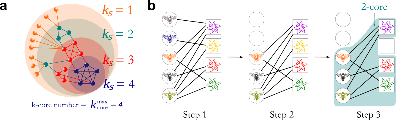
Fig. 1:

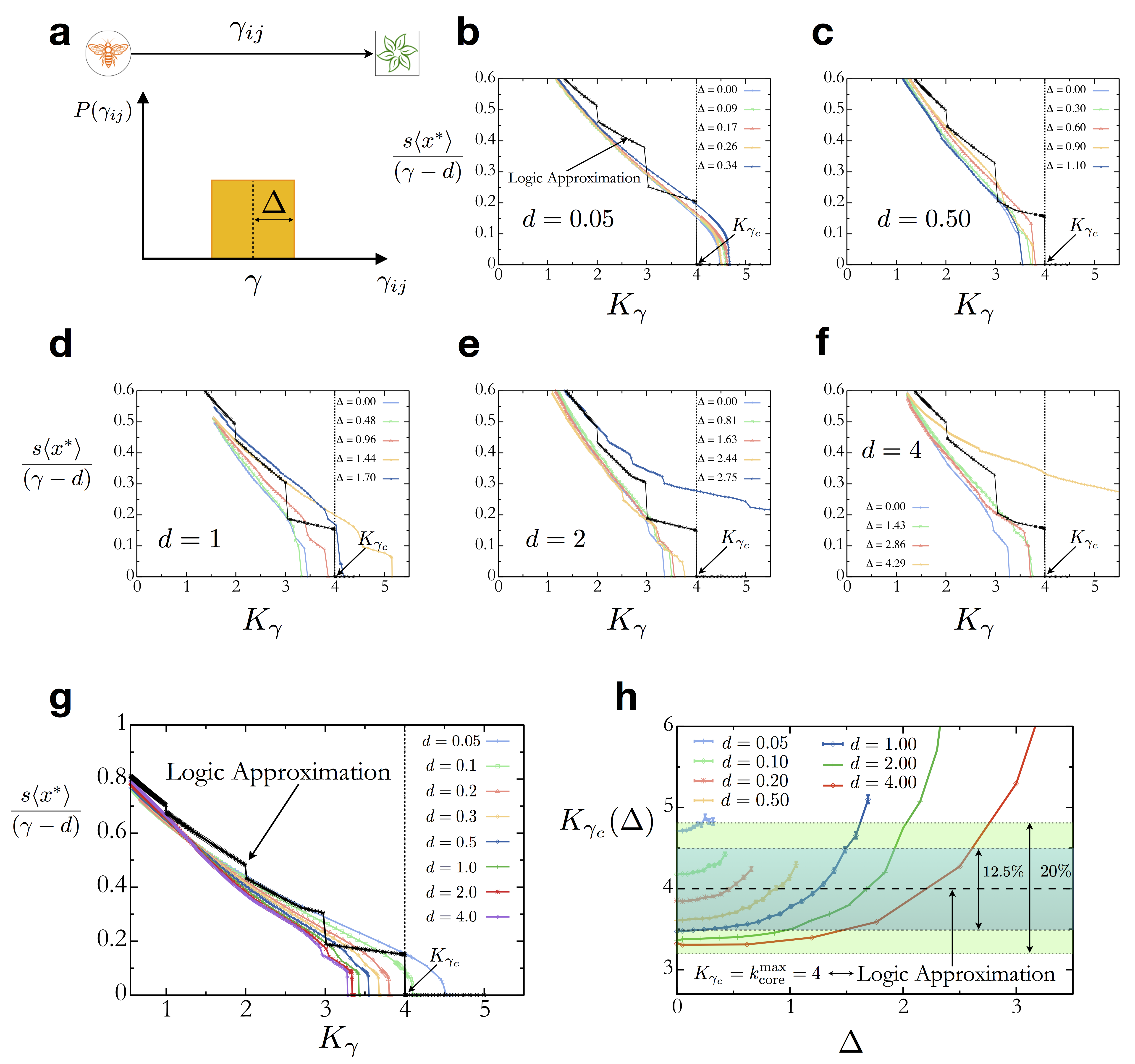
Fig. 2:

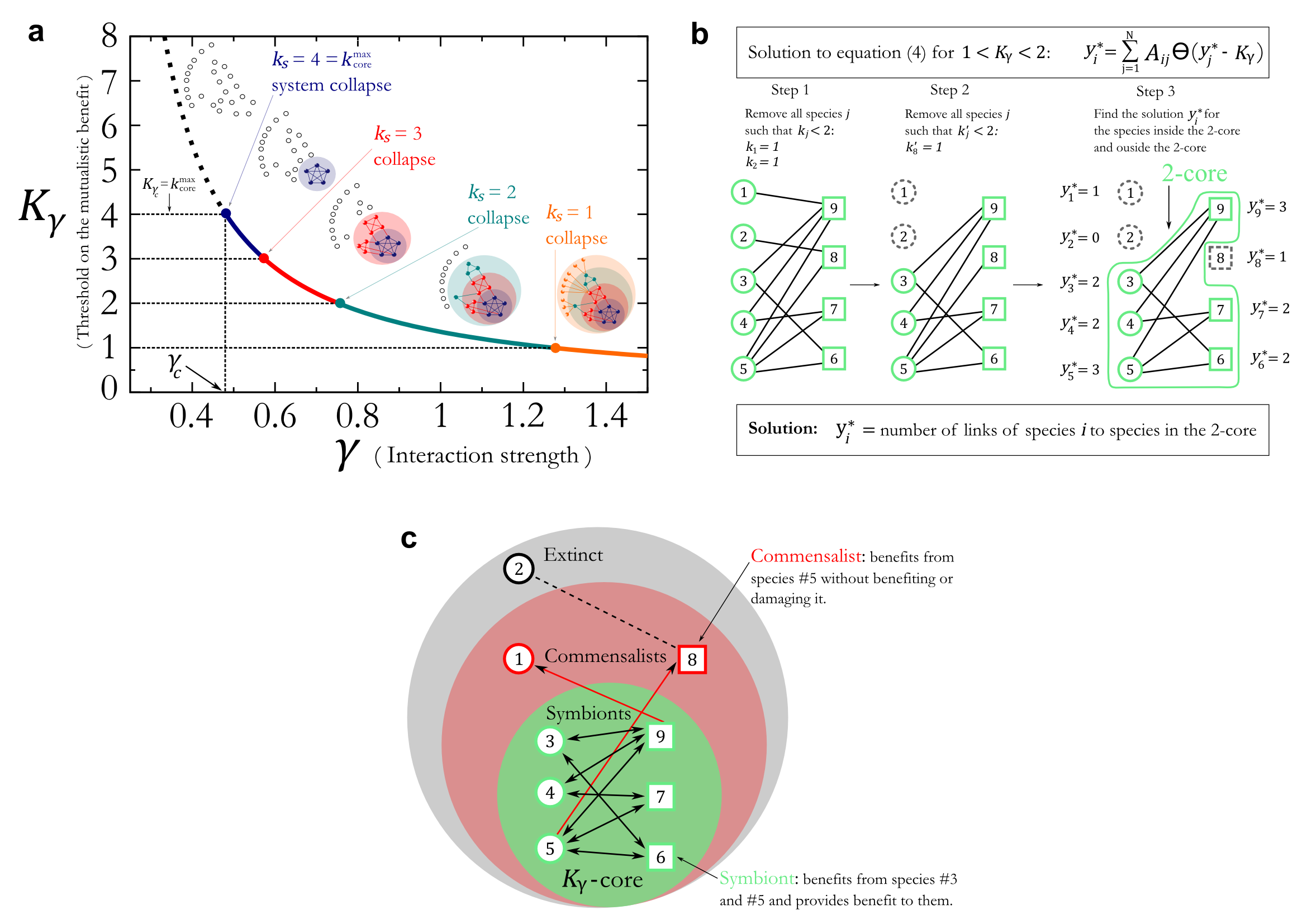
Fig. 3:

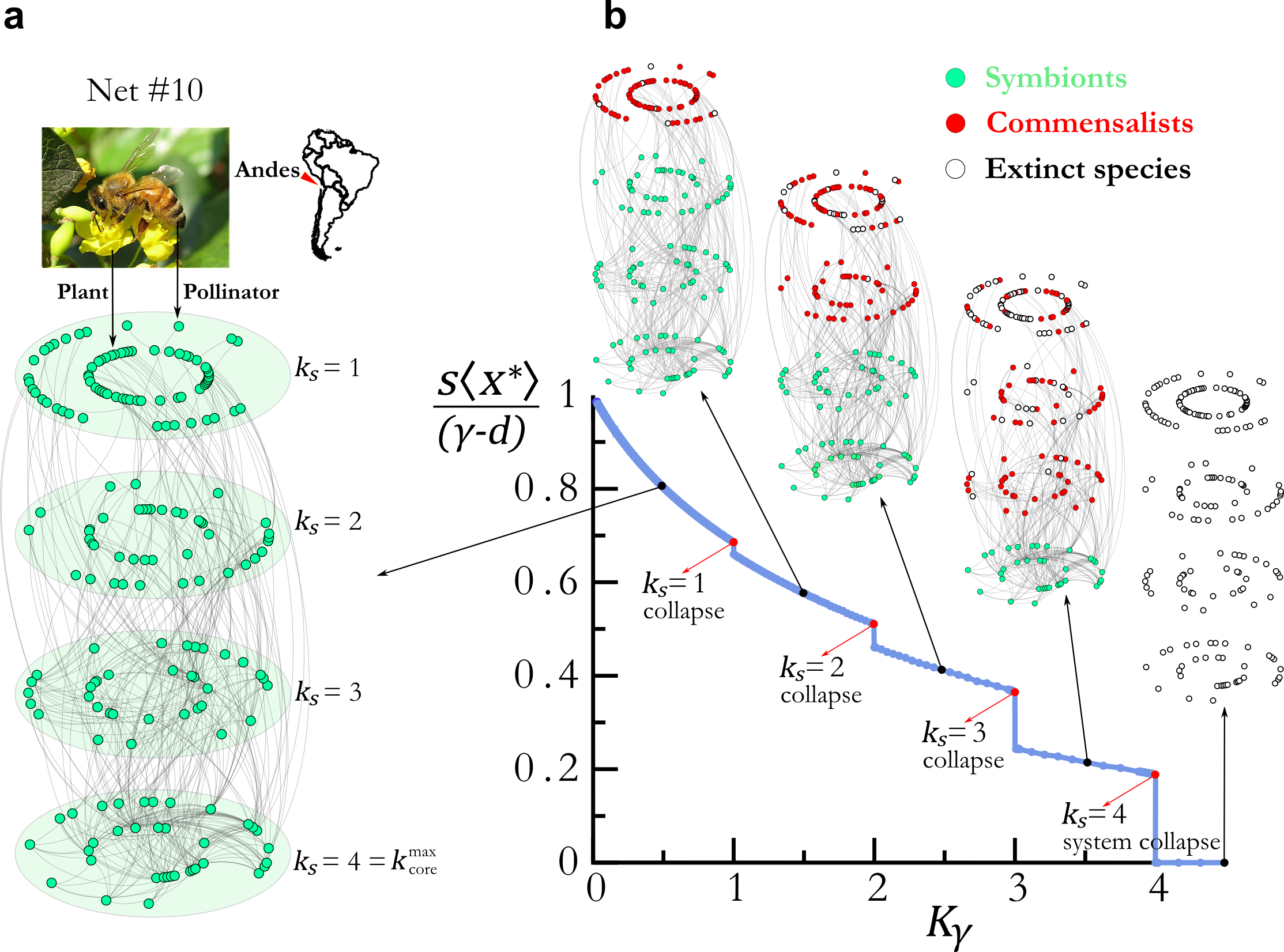
Fig. 4:

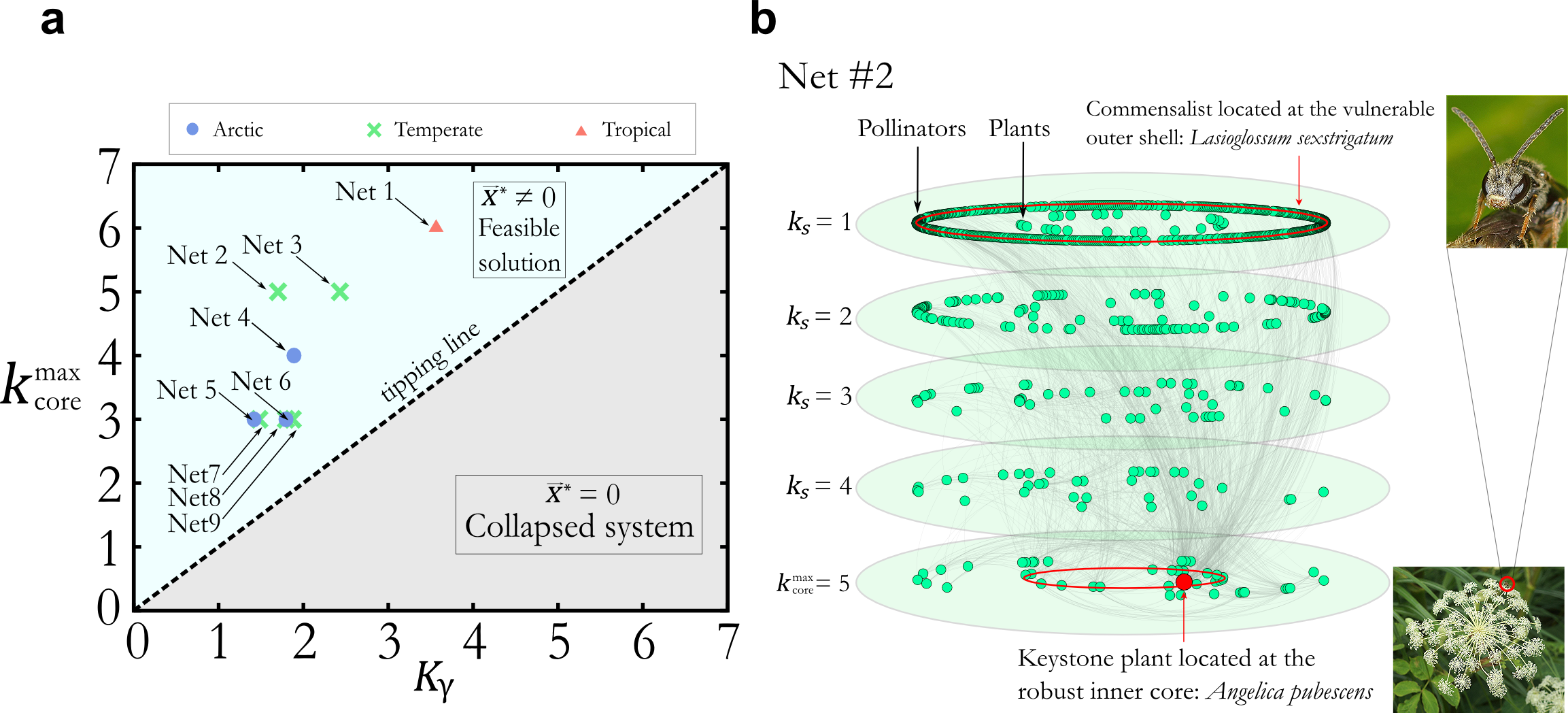
Fig. 5:

Supplementary Information for:

The k-core as a predictor of structural collapse in mutualistic ecosystems

Flaviano Morone, Gino Del Ferraro, and Hernán A. Makse

Contents

1. I Introduction
2. II Model of a mutualistic ecosystem
3. III Numerical analysis of the ecosystem collapse
4. IV Analytical solution of the ecosystem collapse
5. V Tipping point predicted by the maximum k-core of the network
6. VI Stability analysis and phase diagram of system feasibility
7. VII Summary
8. VIII Methods
   1. VIII.1 Numerical integration
9. I Definition of k-core, k-shell and k-core number $k_{\rm core}^{\rm max}$
10. II Gene regulatory networks and neural networks
    1. II.1 Gene regulatory networks
    2. II.2 Neural networks
11. III Numerical solution in mutualistic weighted and directed networks
12. IV Analysis of empirical mutualistic networks
13. V Derivation of the fixed point solution (6)
    1. V.1 Example of solution for systems with 2, 3 and 4 species
14. VI Limits of validity of the approach
    1. VI.1 Test of the logic approximation
    2. VI.2 Test of theoretical predictions for other types of interaction terms used in dakos
    3. VI.3 Test of right-skewed distribution of $\gamma_{ij}$ from Bascompte et al. bascompte-linear
    4. VI.4 Test of non identical death rates and self-limiting parameters
    5. VI.5 Test of predictions of collapse
    6. VI.6 Comparison with other metrics
    7. VI.7 Other limits of validity
    8. VI.8 Changes in death rate
    9. VI.9 Other comparisons
15. VII Stability of the fixed point solution
    1. VII.1 Stability analysis of Ref. may3

I Definition of k-core, k-shell and k-core number $k_{\rm core}^{\rm max}$

The k-core of the network is topologically defined as the maximal subgraph, not necessarily globally connected, consisting of nodes having degree at least $k$ seidman ; dorogotsev . This subgraph is unique and can be extracted by iteratively pruning nodes with degree less than $k$. By definition, the k-core contains the higher order k+1-core, so the 1-core contains the 2-core, the 2-core contains the 3-core, and so on. Each k-core is composed by the nodes at the periphery called k-shell and labeled $k_{s}$, and the remaining k+1-core. The periphery of the k-core is defined as the subgraph induced by nodes and links in the k-core and not in the k+1-core. See Figs. 1a and 1b for examples of how to calculate the k-cores.

In particular, the 1-shell is a forest, i.e., a collection of trees. The value $k_{\rm core}^{\rm max}$ of the largest order k-core, which coincides with the largest value of the k-shell index $k_{s}$, is called the k-core number of the network and it corresponds to the innermost core of the network. It is a topological invariant of the network, meaning that it does not depend on how the nodes are labeled or the network portrayed, i.e., it is invariant under homeomorphisms. Interestingly, the k-core number is also related to the chromatic number of the network $\chi$ (defined as the minimum number of colors to color the nodes so that no neighboring nodes have the same color), in that $k_{\rm core}^{\rm max}$ provides a bound for $\chi$, i.e., $\chi\leq 1+k_{\rm core}^{\rm max}$ szekeres . In particular a network is $\chi$-colorable if it does not have a $\chi$-core (but the converse is not always true).

II Gene regulatory networks and neural networks

The specific form of the coupling term in the mutualistic system defined by Eqs. (1) raises the question of what are the main ingredients necessary for the importance of the k-core for the tipping point. Thus, it is important to understand how the specific form of the coupling term in Eqs. (1) affects the main conclusion that the k-core determines the tipping point of the system. The model of Eqs. (1) is widely used in ecology holland ; thebault ; may ; bastolla ; holland3 to describe mutualistic interactions between species and was put forward in bastolla , and then used subsequently by others to study the stability of ecosystems thebault . The crucial ingredient of the model is the particular analytic form of the coupling function of the form $x_{i}x_{j}/(\alpha+\sum_{k}A_{ik}x_{k})$. We find that the relevance of the k-core to predict the tipping point is more general than this particular interaction term. The analytical results are still valid as long as the interaction term saturates at large values.

For instance, in this Supplementary Information Section II.1, we show that the collapse is predicted by the k-core for a system interacting via a simpler Hill function coupling of the form $x_{j}^{n}/(\alpha^{n}+x_{j}^{n})$, which describes expression levels of gene products in transcriptional networks and in enzymatic reactions alon ; alon1 ; alon3 ; kauffman ; kauffman2 ; gao . Likewise, we show in this SI Section II.2, that other types of sigmoidal interactions that model the coupling of firing neurons in neural networks amit ; sompolinsky ; gao : $[1+\tanh(n(x_{j}-\alpha))]$, where $\alpha$ is the firing threshold, and $n$ describes the slope of the sigmoid function, also retains the same dependence, in general terms, of the tipping point on the k-core as the model of Eqs. (1).

Below we study these two classes of dynamical systems with different couplings: gene regulatory networks and neural networks which show the same type of behaviour as the mutualistic system. All the systems are described by general response functions that saturate at large values. It is important to note that below we focus only on the importance of the shape of the saturating coupling term for the kcore solution. In particular, we show at the end of this SI Section VII.1, that when one considers the typical linear term of interaction used in other studies of ecosystems may3 ; allesina ; bascompte-linear ; coyte , then a different solution is found with paradoxical results known as the stability-diversity paradox may3 .

Furthermore, in the following examples, we keep the strong condition that all interactions needs to be positive. Thus, we consider gene regulatory networks where all genetic interactions are activators and neural systems of excitatory neurons. Thus, no repressor or inhibitory interactions are considered in the examples below. This allows us to map the dynamical problem to a static problem like k-core percolation, with the concomitant importance of the giant k-core. As mentioned in the main text, systems with excitatory and inhibitory interactions requires a more general theory beyond percolation, that is presented elsewhere.

As discussed in the main paper, a functional response widely used in biology and ecology to model the rate at which $x_{i}(t)$ changes as a consequence of the interaction with $x_{j}(t)$ is the Hill function $H_{n}(x_{j})=x_{j}^{n}/(\alpha^{n}+x_{j}^{n})$ alon ; holland .

The parameter $\alpha$ is the activation coefficient, which defines the minimal density $x_{j}$ needed to significantly activate the interaction. The parameter $n$ is the Hill coefficient governing the steepness of the functional response.

In models of neural networks a popular choice for the functional response is $G(x_{j})=\frac{1}{2}[1+\tanh(n(x_{j}-\alpha))]$ amit , where $\alpha$ is the firing threshold, and $n$ describes the slope of the sigmoid function. In particular, for $n\to\infty$, $G(x_{j})$ takes only two discrete values $0$ or $1$, meaning that the neuron is inactive or firing at the maximum rate and corresponds to the logic approximation used in Boolean gene networks introduced by Kauffman kauffman ; kauffman2 and employed in the main text.

In general, we can extend the study of the system defined in the main text to three additional types of dynamical systems used in the literature, where the main feature is how the rate of change of the activity $x_{i}(t)$ is modeled by a sigmoidal type of response function alon ; gao ; holland ; thebault ; amit :

$${\rm I}\ \ \dot{x_{i}}(t) =\ -x_{i}(d+sx_{i})+\sum_{j=1}^{N}A_{ij}\gamma_{ij}x_{i}\frac{x_{j}^{n}}{\alpha^{n}+x_{j}^{n}}\hskip 79.6678pt{\rm simplified\ mutualistic\ coupling},$$ (11)

$${\rm II}\ \ \dot{x_{i}}(t) =\ -dx_{i}+\gamma\sum_{j=1}^{N}A_{ij}\frac{x_{j}^{n}}{\alpha^{n}+x_{j}^{n}}\hskip 133.72786pt{\rm gene\ regulation},$$

$${\rm III}\ \ \dot{x_{i}}(t) =\ I-\frac{x_{i}}{R}+\frac{J}{2}\sum_{j=1}^{N}A_{ij}\Big{[}1+\tanh(n(x_{j}-\alpha))\Big{]}\hskip 56.9055pt{\rm neural\ networks}.$$

In the case of neural networks the constants are defined as $I$: the basal activity, $R$: the inverse of the death rate, and $J$ the strength of the interactions. Below we elaborate on these models and show that the k-core determines the tipping point in all of them.

II.1 Gene regulatory networks

We first study gene regulatory networks governed by the Michaelis-Menten equation alon ; gao ; karlebach , where the rate of change of gene expression $x_{i}(t)$ can be described by the Hill equation  alon ; gao :

$$\ \dot{x_{i}}(t) =\ -dx_{i}\ +\ \gamma\sum_{j=1}^{N}A_{ij}\frac{x_{j}^{n}}{\alpha^{n}+x_{j}^{n}}\hskip 28.45274pt{\rm gene\ regulation}\ ,$$ (12)

where $d>0$ is the mortality rate of the genes, $\gamma$ is the maximal interaction strength between pair of genes, and the activation coefficient $\alpha>0$ defines the minimal expression activity $x_{j}$ needed to significantly activate the interaction. The exponent $n$ of the Hill coefficient governs the steepness of the Hill functional response $H_{n}(x_{j},\alpha)$, which is taken as $n=2$ or higher gao ; alon , thus assuring that the logistic approximation is well posed kauffman ; kauffman2 .

To solve the fixed point equations, we thus use the logic approximation of the Hill function alon ; amit ; kauffman as in the main text, $H_{n}(x_{j})\approx\Theta(x_{j}-\alpha)$, which is exact for $n\to\infty$. The step function $\Theta(x)$ equals $1$ if $x>0$ and zero otherwise. The nonzero fixed point is then:

$$x_{i}^{*}\ =\ \frac{\gamma}{d}\sum_{j=1}^{N}A_{ij}\Theta(x_{j}^{*}-\alpha)\ ,\ \ \ \ i=1,\dots,N\ ,$$ (13)

where, for simplicity, we choose uniform dynamical parameters. Supplementary Eqs. (13) may be conveniently rewritten using the auxiliary variables as in the main text, $y_{i}^{*}=x_{i}^{*}d/\gamma$, and the threshold $K_{\gamma}=(\alpha d)/\gamma$ as

$$y_{i}^{*}\ =\ \sum_{j=1}^{N}A_{ij}\Theta(y_{j}^{*}-K_{\gamma})\ ,\ \ \ \ i=1,\dots,N\ .$$ (14)

The threshold $K_{\gamma}$ in Supplementary Eqs. (14) is the bifurcation parameter whose changes produce quantitative and qualitative changes of the fixed point solution.

The solution in this case is obtained in the same way as done in the main text for the mutualistic ecosystem. First of all, notice that $y_{j}^{*}$ can assume only integer values in the set $y_{j}^{*}\in\{1,\dots,k_{j}\}$ due to the discrete nature of the step functions, where $k_{j}$ is the degree of node $j$. For a given value $K_{\gamma}$, we eliminate all the variables $y_{j}^{*}$ for which $k_{j}<K_{\gamma}$, since these variables give a vanishing contribution to the r.h.s. of Supplementary Eqs. (14), and we only solve for the remaining ones. After this first removal, nodes have smaller degrees $k_{j}^{\prime}$, and if $k_{j}^{\prime}<K_{\gamma}$ a new removal occurs until the degrees of all the remaining nodes are larger than or equal to $K_{\gamma}$. This process is identical to the algorithm for extracting the $\lceil K_{\gamma}\rceil$-core of the network dorogotsev ; gallos . Thus, the nodes left at the end of the pruning process, if there are, form a $K_{\gamma}$-core by construction. The solution to the reduced system then is obtained by setting all the $\Theta$-functions to $1$, and reads

$$y_{i}^{*}\ =\ {\rm numbers\ of\ }i{\rm{}^{\prime}s\ neighbors\ \in\ }\lceil K_{\gamma}\rceil-{\rm core}\ ,$$ (15)

which is consistent because $\Theta(y_{i}^{*}-K_{\gamma})=1$ and we use the notation: $\mathcal{N}_{i}(K_{\gamma})\equiv{\rm number\ of\ }i{\rm{}^{\prime}s\ neighbors\ \in\ }\lceil K_{\gamma}\rceil{\rm-core}$. Now we put back in Supplementary Eqs. (14) the eliminated variables. Since they do not give any contribution to the r.h.s. of Supplementary Eqs. (14), the solution Supplementary Eqs. (15) for the in-core variables remains valid also in the full system. Moreover, the solution Supplementary Eqs. (15) is valid also for the out-core variables, since the nonzero contribution they receive comes from the in-core variables only. Therefore, the expression of a gene outside the $\lceil K_{\gamma}\rceil$-core may be non-zero only if it interacts with at least one of the $\lceil K_{\gamma}\rceil$-core genes.

As in the case of mutualistic networks, the tipping point of collapse of the gene regulatory network is obtained at the critical threshold $K_{\gamma_{c}}$:

$$k_{\rm core}^{\rm max}\ =\ K_{\gamma_{c}}\ \ \to\ \ k_{\rm core}^{\rm max}\ =\ \frac{\alpha d}{\gamma_{c}},$$ (16)

which relates the k-core number $k^{\rm max}_{\rm core}$ of the regulatory network and the dynamical parameters. As in mutualistic ecosystems, the network structure enters in Supplementary Eq. (16) only through the global topological index $k_{\rm core}^{\rm max}$, while local details of the network, like the degrees of individual nodes, are inessential at the critical point.

II.2 Neural networks

Here we study neural networks governed by the following dynamics amit ; sompolinsky :

$$\dot{x_{i}}(t)\ =\ I-\frac{x_{i}}{R}+\frac{J}{2}\sum_{j=1}^{N}A_{ij}\Big{[}1+\tanh(n(x_{j}-\alpha))\Big{]}\ \ \ \ {\rm neural\ networks}\ ,$$ (17)

where $I$ is the basal activity of the neurons, $R$ is the inverse of the death rate, $\alpha$ is the firing threshold, and $J$ is the maximal interaction strength between pair of neurons. The coefficient $n$ governs the steepness of the sigmoid function, analogously to the Hill coefficient $n$ in gene regulatory networks.

To solve the fixed point equations, we use the logistic approximation of the response function, $\frac{1}{2}\Big{[}1+\tanh(n(x_{j}-\alpha))\Big{]}\approx\Theta(x_{j}-\alpha)$, which is exact in the limit $n\to\infty$. The fixed point equations then read:

$$x_{i}^{*}\ =\ IR+JR\sum_{j=1}^{N}A_{ij}\Theta(x_{j}^{*}-\alpha)\ .$$ (18)

Supplementary Eqs. (18) can be rewritten using the auxiliary variable $y_{i}^{*}=(x_{i}^{*}-IR)/(JR)$ and the threshold $K_{J}=\alpha/(JR)-I/J$ as

$$y_{i}^{*}\ =\ \sum_{j=1}^{N}A_{ij}\Theta(y_{j}^{*}-K_{J})\ ,$$ (19)

which is in the same form of Supplementary Eqs. (14). Therefore, we can derive the solution of Supplementary Eqs. (19) by following the same steps after Supplementary Eqs. (14). Thus we find:

$$y_{i}^{*}\ =\ {\rm numbers\ of\ }i{\rm{}^{\prime}s\ neighbors\ \in\ }\lceil K_{J}\rceil-{\rm core}\ .$$ (20)

As in mutualistic and gene regulatory networks, the k-core plays a crucial role in the dynamics of neural networks as well. In particular, the tipping point of collapse of the neural network is obtained when $K_{J}$ equals the k-core number of the neural network:

$$k_{\rm core}^{\rm max}\ =\ K_{J_{c}}\ \ \to\ \ k_{\rm core}^{\rm max}\ =\ \frac{\alpha-IR}{J_{c}R}\ ,$$ (21)

which connects the structure of the neural network, via the k-core number $k_{\rm core}^{\rm max}$, to the dynamical parameters, in particular the critical interaction strength $J_{c}$.

III Numerical solution in mutualistic weighted and directed networks

Interaction strengths between species are, in general, weighted and directed, so that $\gamma_{ij}\neq\gamma_{ji}$. In this general case it is not possible to find the analytical solution to the fixed point equations, so we need to compute this solution numerically. The fixed point equations of the dynamical system Eqs. (1) read:

$$x_{i}^{*}\ =\ -\frac{d}{s}+\frac{1}{s}\sum_{j=1}^{N}A_{ij}\gamma_{ij}\frac{x_{j}^{*}}{\alpha+\sum_{j=1}^{N}A_{ij}x_{j}^{*}}\ ,\ \ \ \ i=1,\dots,N\ ,$$ (22)

where, as we said, $\gamma_{ij}\neq\gamma_{ji}$ and $A_{ij}\neq A_{ji}$. As we explained in the main text, the interactions strengths $\gamma_{ij}$ are independent and identically distributed random variables drawn from a uniform distribution $P(\gamma_{ij})$ with mean $\gamma$ and width $\Delta$:

$$P(\gamma_{ij})\ =\ \frac{1}{2\Delta}[\Theta(\gamma_{ij}-\gamma+\Delta)-\Theta(\gamma_{ij}+\gamma-\Delta)]\ ,$$ (23)

where $\Delta$ takes value in the interval $\Delta\in[0,\Delta_{\rm max}]$. For $\Delta=0$, the interaction strengths $\gamma_{ij}$ are unweighted, i.e., $\gamma_{ij}=\gamma$. On the other side, for $\Delta=\Delta_{\rm max}$ the interaction strengths are maximally heterogeneous, since $\Delta_{\rm max}$ is the maximum admissible width compatible with mutualistic interactions, i.e., such that all $\gamma_{ij}$ are non-negative, $\gamma_{ij}\geq 0$. Next we explain the procedure to compute the solution to the fixed point Supplementary Eqs. (22) and how to get the profiles of the curves in Figs. 2b-f.

1. For a given $d\in[0.05,4.0]$, $\gamma\in[0,\infty)$ and $\Delta\in[0,\Delta_{\rm max}]$ we draw a sample of $\{\gamma_{ij}\}$ from the distribution in Supplementary Eq. (23) and we assign to each directed link the interaction strength $\gamma_{ij}$. We use $\alpha=1$, and $s=1$.

2. Using the so defined set of $\{\gamma_{ij}\}$ we integrate numerically the dynamical Eqs. (1) using a $4^{\rm th}$-order Runge-Kutta algorithm until all the variables $x_{i}(t)$ reach the steady state $x_{i}(t)=x_{i}^{*}$, which is the solution to the fixed point Supplementary Eqs. (22). In the Runge-Kutta algorithm we use a time step $\Delta t=0.01$ and we iterate the algorithm until the steady state sets in in around $10^{5}$ time steps. We initialize the densities $x_{i}(0)>0$ at time $t=0$ uniformly at random.

3. We decrease $\gamma$ and repeat step (1) and (2) until the system reaches the tipping point of collapse, that is, the fixed point $x_{i}^{*}=0$ for all $i$. We denote with $\gamma_{c}(\Delta)$ the critical value of $\gamma$ where the system collapses, and we highlight that it depends on $\Delta$.

Thus, following the steps 1-3 we obtain the fixed point solution as a function of $\gamma$ for a given $\Delta$, that is $x_{i}^{*}=x_{i}^{*}(\gamma)$. We measure, in the steady state, the average fixed point density $\langle x^{*}\rangle=\frac{1}{N}\sum_{i=1}^{N}x_{i}^{*}$. In Fig. 2b we show the results of the rescaled average density of species $\frac{s\langle x^{*}\rangle}{\gamma-d}$ as a function of $K_{\gamma}$ for several values of $\Delta$ and $d=0.05$, using the network #10 in Supplementary Table 1 obtained from Ref. arroyo . Similarly, by changing the value of $d\in[0.05,4.0]$, and repeating the steps 1-3, we obtain all other curves depicted in Fig. 2c-f. Figure 2g shows a similar integration, for several values of $d\in[0.05,4.0]$ with the distribution width $\Delta=0$.

In Fig. 2h we show the behaviour of the parameter $K_{\gamma_{c}}(\Delta)\sim 1/\gamma_{c}(\Delta)$ as a function of $\Delta$ for several values of $d\in[0.05,4.0]$. The critical parameter $K_{\gamma_{c}}(\Delta)$ (critical interaction strength $\gamma_{c}(\Delta)$) is defined at the value of $\gamma$ for which the average density of species $\langle x^{*}\rangle$ jumps to zero.

IV Analysis of empirical mutualistic networks

Supplementary Table 1 summarizes the information about the real mutualistic networks used in Figs. 2, 3, 4, 5. All the networks analyzed in this work can be downloaded from the Interaction Web Database at https://www.nceas.ucsb.edu/interactionweb/; a nonprofit cooperative database of published data on species interaction networks hosted by the National Center for Ecological Analysis and Synthesis, at the University of California, Santa Barbara, US. This database provides datasets on species interactions from communities around the world. Currently available data are for a variety of interaction types, including plant-pollinator, plant-frugivore, plant-herbivore, plant-ant mutualists and predator-prey interactions. These data come from studies in which all species in a particular location, or a substantial subset, were studied and interactions recorded. The networks are bipartite webs: species in one group are assumed to interact with species in the other group but not with species in their own group (e.g., plants and pollinators). Each dataset is defined by an interaction adjacency matrix $A_{ij}$, in which columns represent one group (e.g., plants) and rows represent the other group (e.g., pollinators). We then define the networks of interacting species via the adjacency matrix $A_{ij}$, which is equal to $1$ if species $i$ and $j$ interact, and $0$ otherwise, from where we extract the k-core structure of the network.

From this database, we consider only data in the literature for ecosystems where the full interaction graph $A_{ij}$ has been measured together with the interaction strength $\gamma$ in order to plot the networks in the phase diagram of Fig. 5a and test the feasible-stable condition of Eq.  (9) predicted by the theory. The interaction strength $\gamma$ is measured in the field by counting the frequency of visits of a pollinator to a plant bascompte-linear , and the actual values can be found in the Supplementary Information of Ref. bascompte-linear . The values of the remaining dynamical parameters can be found in Ref. okuyama and in the Supplementary Table S1 of Ref. thebault .

The resulting set of real networks is a robust and broad dataset, comprising of systems located at different latitudes, like Artic, Temperate and Tropical, different locations from Japan, Australia, USA to the Chilean Andes and beyond, of relatively large sizes ranging up to 679 species made of systems of plant-pollinators and plant-seed dispersers displaying relatively large and robust k-core structures ranging from $k_{\rm core}^{\rm max}=3$ to 6, as plotted in Fig. 5a. We notice that the larger the maximum k-core of the system, the more robust the system is. That is, for larger $k_{\rm core}^{\rm max}$, the system can accommodate a larger decrease in interaction strength $\gamma$ without collapsing, as seen in Fig. 5a in the shape of the tipping line in the phase diagram. These unique datasets that combine network structure and interaction strengths are ideal to test the predictions of our phase diagram in Fig. 5a, and supports the main prediction of the theory regarding the feasible-stable state of ecosystems.

Net #	Network type	Plants	Animals	Latitude	Location	Ref.
1	Plant-Seed Disperser	31	9	Tropical	Papua New Guinea	beehl
2	Plant-Pollinator	91	679	Temperate	Japan	kato
3	Plant-Pollinator	42	91	Temperate	Australia	ino
4	Plant-Pollinator	23	118	Artic	Sweden	elb
5	Plant-Pollinator	11	18	Artic	Canada	mos
6	Plant-Pollinator	14	13	Temperate	Mauritius Island	ole
7	Plant-Pollinator	7	32	Temperate	USA	schem
8	Plant-Pollinator	29	86	Artic	Canada	hocki
9	Plant-Seed Disperser	12	14	Temperate	Britain	soren
10	Plant-Pollinator	87	99	Temperate	Andes (Chile)	arroyo

Supplementary Table 1: Details of the 9 mutualistic networks used in the phase diagram of Fig. 5a (#1-9) and the network # 10 used in Fig. 2 and Fig. 4b.

V Derivation of the fixed point solution (6)

In this section we show how to derive Eqs. (4) from the nonlinear Eqs. (1), which in turns leads to the solution Eqs. (6) in terms of the k-core of the network.

From Eqs. (1), there is a trivial fixed point $x_{i}^{*}=0$ for all $i$. This corresponds to the extinction of all species. The nontrivial fixed point $x_{i}^{*}\neq 0$ which corresponds to the extant species satisfying Eqs. (6) is obtained as follows. The equation of the non-trivial fixed point for the dynamical system in Eqs. (1) with $\gamma_{ij}=\gamma$ reads:

$$x_{i}^{*}\ =\ -\frac{d}{s}+\frac{\gamma}{s}\sum_{j=1}^{N}A_{ij}\frac{x_{j}^{*}}{\alpha+\sum_{j=1}^{N}A_{ij}x_{j}^{*}}\ ,\ \ \ \ i=1,\dots,N\ .$$ (24)

The trick to find the solution is to turn this set of equations into a form that can be casted in terms of the Hill function. Then we set:

$$b\ =\ \frac{d}{s},$$ (25)

$$c\ =\ \frac{\gamma}{s}\ ,$$

$$z_{i}^{*}\ =\ \sum_{i=1}^{N}A_{ij}x_{j}^{*}\ ,$$

so that Supplementary Eqs. (24) can be rewritten as

$$z_{i}^{*}\ =\frac{\alpha(b+x_{i}^{*})}{(c-b)-x_{i}^{*}}\ =\ \sum_{i=1}^{N}A_{ij}x_{j}^{*}\ .$$ (26)

Next, we eliminate $x_{j}^{*}$ in favor of $z_{j}^{*}$ in the right hand side of Supplementary Eqs. (26) and we get

$$z_{i}^{*}\ =\ \frac{\gamma-d}{s}\sum_{i=1}^{N}A_{ij}\frac{z_{j}^{*}-\frac{\alpha d}{\gamma-d}}{\frac{\alpha\gamma}{\gamma-d}+z_{j}^{*}-\frac{\alpha d}{\gamma-d}}\ .$$ (27)

Finally, we set

$$y_{i}^{*}\ =\ z_{i}^{*}\frac{s}{\gamma-d}\ ,$$ (28)

and we obtain:

$$y_{i}^{*}\ =\ \sum_{j=1}^{N}A_{ij}\frac{(\gamma-d)^{2}y_{j}^{*}-\alpha ds}{\alpha\gamma s+(\gamma-d)^{2}y_{j}^{*}-\alpha ds}\ .$$ (29)

This equations can be written in terms of the Hill function, $H_{n}(x,T)$, which is commonly used to describe interactions of species from ecosystems to biological systems alon ; amit ; kauffman ; kauffman2 :

$$H_{n}(x,T)=\frac{x^{n}}{T^{n}+x^{n}}\ ,$$ (30)

where $T=\frac{\alpha\gamma s}{(\gamma-d)^{2}}$ is the half saturation constant and $n$ is the Hill coefficient. Using the Hill function, we obtain:

$$y_{i}^{*}\ =\ \sum_{j=1}^{N}A_{ij}H_{1}\Bigg{(}y_{j}^{*}-\frac{\alpha ds}{(\gamma-d)^{2}},\ \frac{\alpha\gamma s}{(\gamma-d)^{2}}\Bigg{)}\ .$$ (31)

Supplementary Eqs. (31) cannot be solved analytically for general networks. To find the analytical solution for this fixed point we use the logic approximation of the Hill function, which is widely used in theoretical biology alon ; amit ; kauffman ; kauffman2 :

$$H_{n}(x,T)\approx\Theta(x-T),$$ (32)

and becomes exact in the limit $n\to\infty$, where the step function $\Theta(x)=1$ if $x>0$ and zero otherwise. The fixed point Supplementary Eqs. (31), in the logic approximation, can be written as follows:

$$y_{i}^{*} =\ \sum_{j=1}^{N}A_{ij}\Theta(y_{j}^{*}-K_{\gamma}),$$ (33)

$$K_{\gamma} =\ \frac{\alpha s(\gamma+d)}{(\gamma-d)^{2}}\ ,$$

which is the Eqs. (4) presented in the main text. This set of equations admits an exact solution in the form of Eqs. (6) as explained in the main text. We note that such a solution is valid for any network structure with an arbitrary degree distribution (such as Erdös-Renyi or scale-free networks) or any internal structure such as modularity, hierarchical, nestedness, including locally tree-like and dense networks. Thus, it is the general exact solution to the fixed point equations of the ecosystem dynamics based solely on the logic approximation of the Hill function, which allows one to obtain the analytical solution of the problem in closed form for any network structure. Then, using Supplementary Eqs. (26) and (28), we can also write the nonzero fixed point solution Eqs. (6) in terms of the original species densities $x_{i}^{*}$ as:

$$x_{i}^{*}\ =\ \frac{(\gamma-d)^{2}\mathcal{N}_{i}(K_{\gamma})-\alpha ds}{s^{2}\alpha+s(\gamma-d)\mathcal{N}_{i}(K_{\gamma})}\ ,\ \ \ \ i=1,\dots,N\ .$$ (34)

V.1 Example of solution for systems with 2, 3 and 4 species

In this section we solve the fixed point Eqs. (4) for simple mutualistic ecosystems with 2, 3 and 4 species shown in Supplementary Fig. 1 where the algebra is straightforward. This is done to illustrate the solution in a simple system.

Ecosystem with 2 species. The fixed point equations for the 2-species ecosystem in Supplementary Fig. 1a read:

$$y_{1}^{*} =\ \Theta(y_{2}^{*}-K_{\gamma})\ ,$$ (35)

$$y_{2}^{*} =\ \Theta(y_{1}^{*}-K_{\gamma})\ .$$

The system of Supplementary Eqs. (35) is invariant under a permutation of species 1 and 2, i.e. for $y_{1}^{*}\to y_{2}^{*}$. Therefore, we look for a homogeneous solution $y_{1}^{*}=y_{2}^{*}\equiv y^{*}$ to the single fixed point equation:

$$y^{*}\ =\ \Theta(y^{*}-K_{\gamma})\ .$$ (36)

This equation has the following solution:

$$y^{*} =\ 1\ \ \ \ {\rm if}\ \ 0<K_{\gamma}<1\ ,$$ (37)

$$y^{*} =\ 0\ \ \ \ {\rm if}\ \ K_{\gamma}\geq 1\ ,$$

which can be rewritten using the function $\mathcal{N}(K_{\gamma})$ introduced in the main text as

$$y_{1}^{*}=y_{2}^{*}=y^{*}=\mathcal{N}_{1}(K_{\gamma})=\mathcal{N}_{2}(K_{\gamma})\ .$$ (38)

Indeed, the 2-species ecosystem shown in Supplementary Fig. 1a consists only of the 1-core, hence $k_{\rm core}^{\rm max}=1$. Therefore, when $K_{\gamma}<k_{\rm core}^{\rm max}$, then $y_{1}^{*}$ is equal to the number of links between species 1 and the species in the 1-core $\mathcal{N}_{1}(K_{\gamma})$, which in this case equals 1, since there is only one species connected to species 1 in the 1-core. On the other hand, when $K_{\gamma}>k_{\rm core}^{\rm max}$, the solution is $y_{1}^{*}=y_{2}^{*}=0$, in agreement with the general result presented in the main text. The same reasoning applies to species 2 by swapping the indices $1\to 2$.

Ecosystem with 3 species. The fixed point equations for the 3-species ecosystem in Supplementary Fig. 1b read:

$$y_{1}^{*} =\ \Theta(y_{2}^{*}-K_{\gamma})+\Theta(y_{3}^{*}-K_{\gamma})\ ,$$ (39)

$$y_{2}^{*} =\ \Theta(y_{1}^{*}-K_{\gamma})\ ,$$

$$y_{3}^{*} =\ \Theta(y_{1}^{*}-K_{\gamma})\ .$$

The system of Supplementary Eqs. (39) is invariant under a permutation of species 2 and 3, i.e. for $y_{2}^{*}\to y_{3}^{*}$. Therefore, we look for a solution $y_{1}^{*}\equiv y^{*}$ and $y_{2}^{*}=y_{3}^{*}\equiv z^{*}$ to the following reduced system of equations:

$$y^{*} =\ 2\Theta(z^{*}-K_{\gamma})\ ,$$ (40)

$$z^{*} =\ \Theta(y^{*}-K_{\gamma})\ ,$$

whose solution is:

$$y^{*} =\ 2\ ,z^{*}\ =\ 1\ \ \ \ {\rm if}\ \ 0<K_{\gamma}<1\ ,$$ (41)

$$y^{*} =\ 0\ ,z^{*}\ =\ 0\ \ \ {\rm if}\ \ K_{\gamma}\geq 1\ ,$$

which can be rewritten using the function $\mathcal{N}(K_{\gamma})$ as

$$y_{1}^{*}\ =\ y^{*}\ =\ \mathcal{N}_{1}(K_{\gamma})\ ,$$ (42)

$$y_{2}^{*}\ =\ y_{3}^{*}\ =\ z^{*}\ =\ \mathcal{N}_{2}(K_{\gamma})\ =\mathcal{N}_{3}(K_{\gamma})\ .$$

Indeed, the ecosystem in Supplementary Fig. 1b also consists of just the 1-core, so that $k_{\rm core}^{\rm max}=1$. Then, when $K_{\gamma}<k_{\rm core}^{\rm max}$, $y_{1}^{*}$ is equal to the number of links between species 1 and the other species in the 1-core, that is species 2 and 3, and thus $y_{1}^{*}=2$. Similarly, $y_{2}^{*}$ equals 1, since it is connected only to species 1, and $y_{3}^{*}$ also equals 1 since it is connected only to species 1. Instead, when $K_{\gamma}>k_{\rm core}^{\rm max}$, the system collapses into the trivial fixed point $y_{1}^{*}=y_{2}^{*}=y_{3}^{*}=0$, in agreement with the general solution derived in the main text.

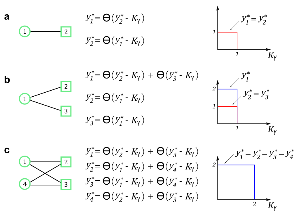
Supplementary Figure 1: Solution to the fixed point equations (4) for small fully connected mutualistic networks. a, Fixed point equations and the corresponding solution for a fully connected mutualistic ecosystem with 2 species. This simple network has only the 1-core, so $k_{\rm core}^{\rm max}=1$. Thus, the system collapses when $K_{\gamma}>1$. The solution for $y_{1}^{*}$ and $y_{2}^{*}$ is given by the number of links connecting species 1 and 2 to the species in the $K_{\gamma}$-core, in agreement with the general solution derived in the main text. b, Fixed point equations and the corresponding solution for a fully connected mutualistic ecosystem with 3 species. This network has only the 1-core, and thus $k_{\rm core}^{\rm max}=1$. Accordingly, the system collapses when $K_{\gamma}>1$. Also in this case the solution for $y_{1}^{*}$, $y_{2}^{*}$ and $y_{3}^{*}$ is given by the number of links connecting species 1, 2 and 3 to the species in the $K_{\gamma}$-core. c, Fixed point equations and the corresponding solution for a fully connected mutualistic ecosystem with 4 species. This network has only the 2-core, and thus $k_{\rm core}^{\rm max}=2$. Therefore, the system collapses when $K_{\gamma}>2$. Also in this case the solution for $y_{1}^{*}$, $y_{2}^{*}$, $y_{3}^{*}$ and $y_{4}^{*}$ is given by the number of links connecting species 1, 2, 3 and 4 to the species in the $K_{\gamma}$-core.

Ecosystem with 4 species. The fixed point equations for the 4-species ecosystem in Supplementary Fig. 1c read:

$$y_{1}^{*} =\ \Theta(y_{2}^{*}-K_{\gamma})+\Theta(y_{3}^{*}-K_{\gamma})\ ,$$ (43)

$$y_{2}^{*} =\ \Theta(y_{1}^{*}-K_{\gamma})+\Theta(y_{4}^{*}-K_{\gamma})\ ,$$

$$y_{3}^{*} =\ \Theta(y_{1}^{*}-K_{\gamma})+\Theta(y_{4}^{*}-K_{\gamma})\ ,$$

$$y_{4}^{*} =\ \Theta(y_{2}^{*}-K_{\gamma})+\Theta(y_{3}^{*}-K_{\gamma})\ .$$

The system of Supplementary Eqs. (43) is invariant under permutations of species 1, 2, 3 and 4. Therefore, we look for a solution $y_{1}^{*}=y_{2}^{*}=y_{3}^{*}=y_{4}^{*}\equiv y^{*}$ to the fixed point equation:

$$y^{*} =\ 2\Theta(y^{*}-K_{\gamma})\ .$$ (44)

This equation has the following solution:

$$y^{*} =\ 2\ \ \ \ {\rm if}\ \ 0<K_{\gamma}<2\ ,$$ (45)

$$y^{*} =\ 0\ \ \ \ {\rm if}\ \ K_{\gamma}\geq 2\ ,$$

which can be rewritten using the function $\mathcal{N}(K_{\gamma})$ as,

$$y_{i}^{*}\ =\ \mathcal{N}_{i}(K_{\gamma})\ =\ 2\ \ \ \ i=1,2,3,4\ .$$ (46)

Indeed, the 4-species ecosystem shown in Supplementary Fig. 1c consists only of the 2-core, hence $k_{\rm core}^{\rm max}=2$. Therefore, when $K_{\gamma}<k_{\rm core}^{\rm max}$, then $y_{i}^{*}$ is equal to the number of links between species $i$ and the species in the $K_{\gamma}$-core, i.e. $\mathcal{N}_{i}(K_{\gamma})$, which in this case equals 2. Finally, when $K_{\gamma}>k_{\rm core}^{\rm max}$ the solution is $y_{i}^{*}=0$ for $i=1,2,3,4$, in agreement with the general solution.

VI Limits of validity of the approach

So far we have studied an oversimplified model of natural ecosystems which allowed us to reach an exact solution in the limit of the logic approximation to produce simple predictions on the tipping point. It is important then to understand the limit of validity of the approach to determine the conditions under which one might expect the approximations to give accurate results, and under what conditions the assumptions are not valid.

In what follows we study the limit of validity of the following approximations as well as perform a comparison with other approaches to predict the tipping point:

• Test of the logic approximation in replacing the $n=1$ Hill function by the Heaviside (Theta) function

• Test of theoretical predictions for other types of interaction terms used in dakos

• Test of predictions for more realistic cases where the interaction strengths $\gamma_{ij}$ are distributed with a right-skewed distribution as found empirically in Bascompte et al. bascompte-linear

• Test of predictions for more realistic cases where the death rates and self-limiting parameters are not identical for all species (pollinators and plants)

• Test of prediction of collapse over different real webs

• Comparison with other metrics

• Test of other conditions that are observed in natural systems like plant-plant interactions and other forms of reproductive modes

• Changes in death rate

• Other comparisons.

VI.1 Test of the logic approximation

One of the most crucial approximations used to derived the k-core solution is the use of the logic approximation. Thus, it is important to understand under which conditions the original $n=1$ Hill function in Supplementary Eqs. (1-3) can be replaced by the Heaviside (Theta) function of the logic approximation.

We solve numerically the fixed point Eqs. (4) obtained under the logic approximation and plot in Fig. 2b-f, as well as in Fig. 2g, the fixed point average density $\langle x^{*}\rangle$ as a function of $K_{\gamma}$, obtained by plugging the result of Eqs. (4) into the Supplementary Eqs. (34) (black line in Figs. 2b-f and in Fig. 2g) . In the same figures, we compare this theoretical prediction with the average density $\langle x^{*}\rangle$ obtained by numerically integrating Eqs. (1) with $\gamma_{ij}$ sampled from a uniform distribution with different width $\Delta$ and at different values of the death rate $d$ . All these numerical calculations are made on the same network of Ref. arroyo .

Using the simulations of Fig. 2 we study how the tipping point $K_{\gamma_{c}}$ obtained numerically for a system with $n=1$ deviates from the prediction of the theory for that particular network, which is $K_{\gamma_{c}}=k^{\rm max}_{\rm core}=4$, for the network used in Fig. 2. The particular form of the distribution of strength $P(\gamma_{ij})$, as a uniform distribution with width $\Delta$, allows us to systematically investigate the logic approximation as a function of the width as well as other parameters. In the next section we will repeat the investigation of the validity of the logic approximation for more realistic distributions of the interactions, such as the right-skewed distribution found in bascompte-linear , and with death rate $d$ and self-limiting parameter $s$ no longer equal across all species.

Each panel 2b-f in Fig. 2 shows the numerical integration of Eqs. (1) for a given value of $d$ as indicated. Each curve shows the integration for a given $\Delta$ and the comparison to the theoretical prediction using the logic approximation $n\to\infty$ and the approximation of unique interaction strength $\gamma$ for all the species. In general, we find that the logic approximation captures well the $n=1$ system for small enough death rates $d$ for any $\Delta$, while for large enough death rate deviations are observed and the logic approximation deviates substantially from the numerical solution. To quantify this situation, in Fig. 2h we plot the numerical tipping point $K_{\gamma_{c}}$ for the $n=1$ system as a function of $\Delta$ and for every system with different $d$. We choose (somehow arbitrary) as a 20% variation as the limit of validity of the theory. Assuming this arbitrary cut off, we find that for $d>2$, and for sufficiently large width of the uniform distribution ($\Delta>1.5$), there are significant deviations from the $K_{\gamma_{c}}=4$ logic approximation prediction (see Fig. 2h, green band). This value marks the limit of validity of the theory.

The reason why the model does not work for large $d$ can be explained by inspection of Eqs. (1). Indeed, a condition of validity of the approach is $d\ll\gamma$. In principle, by definition the species are expected to interact with another species, as a minimum, one time in their lifetime which implies $d<\gamma$. Thus, $d=\gamma$ is the limit of validity of the model. Furthermore, it is realistic to expect (and this is confirmed by values of $d$ in the literature, see below) that species interact many times within each other during their lifetime and, therefore, this constraints the possible values to $d\ll\gamma$. Indeed, typical values of $d$ in the literature are in the range $d\in[0.1-0.3]$, as obtained by Thebault and Fontaine, and Holland et al. thebault ; holland . In this range the tipping point of the $n=1$ system, for the largest $\Delta$, falls in the range $K_{\gamma_{c}}\in[3.7,4.5]$, which is closer to the tipping point predicted by the logic approximation $K_{\gamma_{c}}=4$. At these values of the death rate $d$ the deviation of $K_{\gamma_{c}}$ from the theory reduces to 12.5% (see Fig. 2h, blue band). We then define this latter the limit of validity of the parameter space following the values found in other studies thebault ; holland .

This result suggests that the tipping point of the $n=1$ system in Eqs. (3) can be estimated under the logic approximation of Eqs. (4), which, being analytically tractable, allows us to determine the functional dependence of the tipping point on the network structure and dynamical parameters, as we show next. When the death rate becomes of the order of $\gamma$, then the mutualistic interactions are of the order of the death rate and the model and approximations break down.

To disentangle the effects of both approximations, i.e. the uniform distribution $P(\gamma_{ij})$ and the logic approximation, we plot in Fig. 2g the numerical simulations for $\Delta=0$ with different $d$ values and its comparison with the logic approximation result. We find that in this case the largest deviation of $K_{\gamma_{c}}$ from the theoretical prediction $K_{\gamma_{c}}=k^{\rm max}_{\rm core}=4$ is 17% and appears for the largest as well as the smallest value of $d$ ($d=4$ and $d=0.05$, respectively), both outside the range of experimental $d$-values found in thebault ; holland . For completeness, in Supplementary Fig. 2 we show the same results of Fig. 2g by plotting directly $\langle y^{*}\rangle$ as a function $K_{\gamma}$, obtained by numerically solving Eqs. (4).

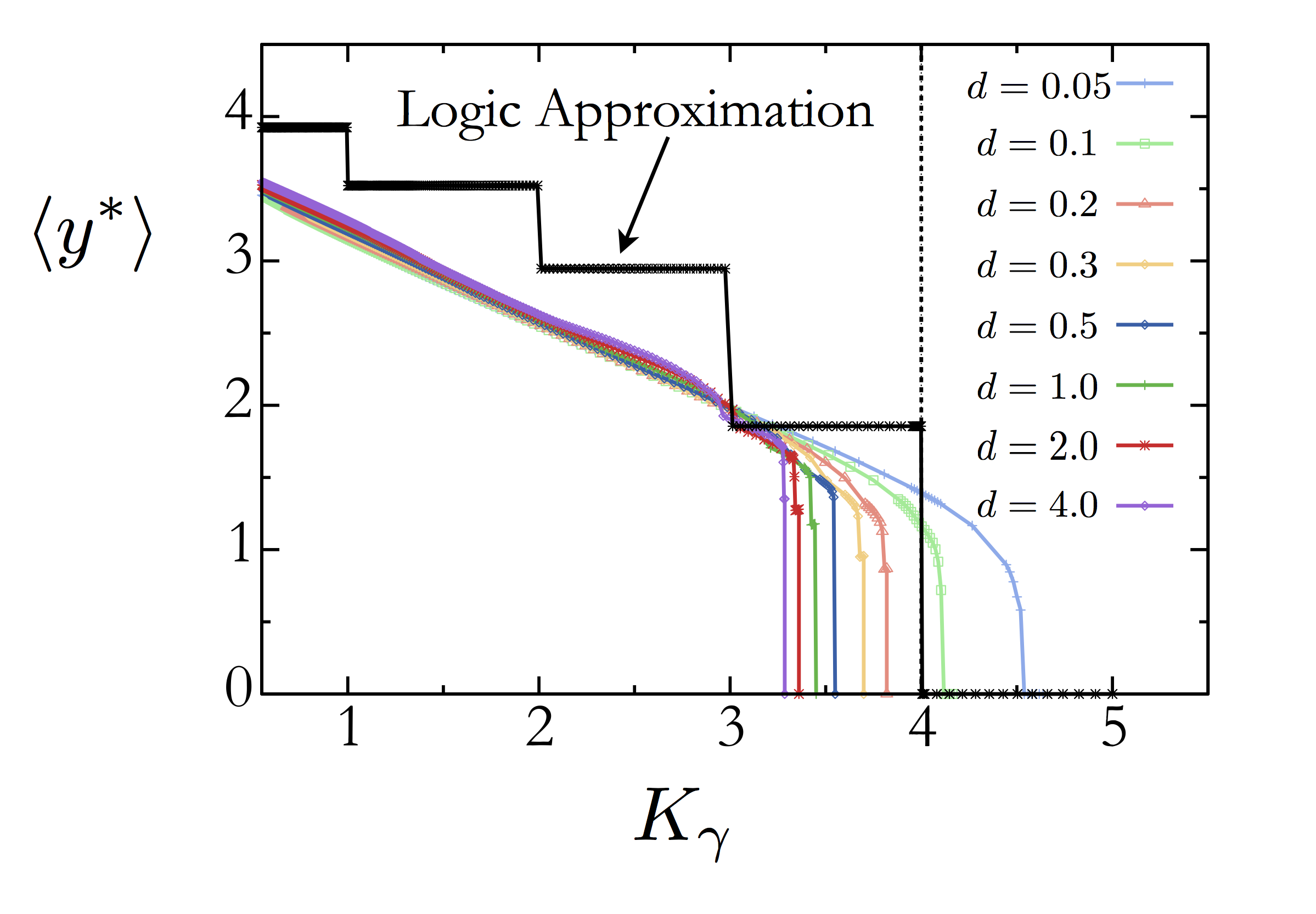
Supplementary Figure 2: Same results as in Fig. 2g, plotted w.r.t. the averaged density $\langle y^{*}\rangle$ obtained from Eqs.(4). Different color lines refer to a numerical integration with a different value of the death rate $d$. The black line illustrates the theoretical solution obtained by iteration of Eqs. (4) till its fixed point. The values of the self-limiting parameter $s$ and the half-saturation constant $\alpha$ are the same as in Figure 2, i.e. $s=1$ and $\alpha=1$.

Let us observe that so far we have studied a critical transition driven by an increase of the parameter $K_{\gamma}$ (or equivalently by a decrease of the interaction strength $\gamma$). In this case the system undergoes an abrupt transition at a tipping point as shown in Fig. 2. Figure 2g shows that the logic approximation predicts an almost linear decrease of the averaged rescaled activity $s<x^{*}>/(\gamma-d)$ before reaching the tipping point at $K_{\gamma_{c}}=4$. Compared to the logic approximation, the numerical solutions in this figure show a slightly different singular behaviour of the average density $s<x^{*}>/(\gamma-d)$ which can still be seen as an increase of the magnitude of the first derivative of $s<x^{*}>/(\gamma-d)$ with respect to $K_{\gamma}$ when approaching the tipping point (for example, at the parameter $d$ equals 0.05 and 0.1).

Yet, when the average density at the fixed point shown in Fig. 2g is plotted in terms of the variable $\langle y^{*}\rangle$ (Supplementary Fig. 2), the numerical solution obtained by integrating Eqs. (1) shows a similar sharp transition at the tipping point to the logic approximation (black line). Between each shell, the activity measured by the logic approximation stays constant and suddenly drops when a given shell goes extinct, i.e. $K_{\gamma}=1,2,3,...$ (see black line in Supplementary Fig. 2). The last jump towards a $\langle y^{*}\rangle=0$ solution in the logic approximation is due to the collapse of the $k_{\rm core}^{\rm max}$ of the system, in this case the $k=4$ core. Differently, the numerical solution does not presents sharp jumps at $K_{\gamma}=1,2,3,$ but shows a progressive linear decrease of the solution (colored lines in Supplementary Fig. 2). The difference of these two behaviors is due to diverse solutions obtained for $n=\infty$ and $n=1$. Indeed, in the numerical solution obtained for $n=1$ the k-shells do not collapse one by one, since the interaction term in the equation of motion is not as sharp as the Heaviside (Theta) function used in the logic approximation. Nevertheless, the transition at the tipping point towards the ecosystem’s collapse is depicted similarly by the two solutions because at this point, even the simulated system passes abruptly from a non-zero solution to a zero or a non-physical solution. This behavior looks similar to the critical behavior observed near critical point of the first-order phase transitions discussed in Refs. shlomo ; sheffer1 ; sheffer2 ; gao which is an evidence for avalanches in the system. Critical behavior is crucially important since it can give early warning signals that may occur near critical points of first-order phase transitions in a wide class of systems. Thus, further refinements of the model should include the study of avalanche behavior as warning of the proximity of the tipping point shlomo ; sheffer1 ; sheffer2 ; gao .

VI.2 Test of theoretical predictions for other types of interaction terms used in dakos

It is also important to understand how the prediction of the k-core for the collapse of the system is affected by different models used in the literature. While Eqs. (1) have been studied in the literature holland ; thebault ; may ; bastolla ; holland3 , other authors have considered modified equations dakos :

$$\dot{x_{i}}(t)\ =\ -dx_{i}-sx_{i}^{2}+\sum_{j=1}^{N}A_{ij}\gamma_{ij}\frac{x_{i}x_{j}}{\alpha+\sum_{k=1}^{N}\gamma_{ik}A_{ik}x_{k}}\ ,\,\,i\in\{1,\cdot\cdot\cdot,N\}\ ,$$ (47)

which represent a proper “Type II” functional response (see for example dakos ). Therefore, it is important to know whether the results holds for this kind of equations as well.

Using the same approximations employed in Eqs. (1) applied to Supplementary Eqs. (47), we find that by a change of variables ($\alpha\to\alpha/\gamma$, and $\gamma=1$) the condition Eq. (7) for collapse now becomes:

$$K_{\gamma_{c}}\ =\ k_{\rm core}^{\rm max}\ \ \to\ \ \frac{\alpha s}{\gamma_{c}}\frac{(1+d)}{(1-d)^{2}}\ =\ k_{\rm core}^{\rm max}\ ,$$ (48)

which represents similar dependence $K_{\gamma_{c}}\approx\alpha s/\gamma_{c}$ as Eqs. (1) in the limit of $d\ll\gamma_{c}$ which is expected experimentally, since the death rate of the species is always smaller than the frequency of interactions thebault ; holland . Supplementary Information Section II discusses other variants of systems of coupled equations with similar conclusions: in all cases the collapse is given by the k-core and the condition of collapse is inversely proportional to the interaction strength in the limit of small death rate.

VI.3 Test of right-skewed distribution of $\gamma_{ij}$ from Bascompte et al. bascompte-linear

In Supplementary Fig. 3a we present the $P(\gamma_{ij})$ distribution experimentally obtained from the data in bascompte-linear which shows a right-skewed shape for the distribution of interaction strengths. Since this distribution is found in Nature, it is of interest to determine whether and how it affects the results of the theory. As for Fig. 2, we integrate Eqs. (1) but this time with the interaction strengths $\gamma_{ij}$ sampled from the empirical distribution of bascompte-linear shown in Supplementary Fig. 3a. In order to span several values of $K_{\gamma}$ and produce the plots in Supplementary Fig. 3, we change the average $\gamma$ by changing the minimal value of the distribution weights accordingly. The underlying network, as for Fig. 2, is the network of Ref. arroyo . Supplementary Fig. 3b shows the results for the case of death rate $d$ and self-limiting parameter $s$ equal across all species. As comparison, we also plot the result of the logic approximation (black line). As the figures shows, the empirical tipping point $K_{\gamma_{c}}$ deviates at most by 20% from the theoretical predicted one, i.e. $K_{\gamma_{c}}=k^{\rm max}_{\rm core}=4$. We observe that, the use of the experimental distribution of bascompte-linear limits the range of parameters which can be explored. Indeed, for the experimental $P(\gamma_{ij})$ as in Supplementary Fig. 3a, the maximum values of $\bar{\gamma}$ is $\bar{\gamma}_{\rm max}=1$ to which correspond a minimum value of $K_{\bar{\gamma}_{\rm min}}=\alpha s(1+d)/(1-d)^{2}$ which, for any $d$, constraints the minimum range of $K_{\bar{\gamma}}$ accessible for the simulations (see the min value of $K_{\gamma}$ in Supplementary Fig. 3b). We further note that, although we have numerically investigated a range of $d$-values $d>0.3$, when integrating Eqs. (1), with $P(\gamma_{ij})$ as in Supplementary Fig. 3a, we have not found any non-trivial solution for this equation for any $d>0.38$. This is the reason why we do not show the same values of $d$ considered in Fig. 2 ($d=0.5,2,4$). However, we observe again that the experimental $d$-values found in thebault ; holland are $d\in[0.1,0.3]$ and are therefore captured by our numerical investigation with a right-skewed $P(\gamma_{ij})$ shown in Supplementary Fig. 3.

VI.4 Test of non identical death rates and self-limiting parameters

In this section we present the results obtained by relaxing the assumption of equal dead rates and self-limiting parameters across species. Following the work of Bascompte et al. bascompte-linear , we sample these parameters from a uniform distribution $P(d_{i})$ and $P(s_{i})$, respectively (see Supplementary Fig. 3c). The average values and the widths of these distributions are chosen from bascompte-linear . From this reference, the average $s$ is taken $s=1$, the $d$-value range therein ($d=1,2$), instead, does not give any non-trivial solution to Eqs. (1), as discussed above. Therefore, we chose $d\in[0.05,0.3]$, as we did for the simulations of Supplementary Fig. 3b, which is within the range of parameters that produces non-trivial numerical solutions of Eqs. (1). The width of $P(d_{i})$ is taken 0, 10, 20, and 30% of its mean value, whereas the width of $P(s_{i})$ is taken 0, 10, and 20% of $\bar{s}$, in agreement with bascompte-linear . The underlying network that we use for the numerical simulation is the same as in Fig. 2 and, as for the simulations presented in SI Section VI.3 and as mentioned above, we do not find any non-zero solution of Eqs. (1) for values of $d>0.37$ (with non-zero width of the distributions). Results are presented in Supplementary Fig. 3d-g for different values of $\bar{d}$. In each panel, each color curve refers to a different value for the width of the $P(d_{i})$ and $P(s_{i})$ distribution, as reported in the legend. In each panel we also show the analytical theoretical prediction obtained with the logic approximation (black line). Overall, we observe that also in the case of $P(\gamma_{ij})$ right-skewed and both death rate and self-limiting parameters not equal across species (the most realistic case for the parameters in the model Eqs. (1)) the theoretical prediction are in good agreement with the numerical ones, within a certain range of validity. As for the results shown in Fig. 2, the largest deviation from the predicted theoretical value $K_{\gamma_{c}}\ =\ k_{\rm core}^{\rm max}=4$ for this network is about 20%, being higher only for larger values of $d$, as $d=0.3$.

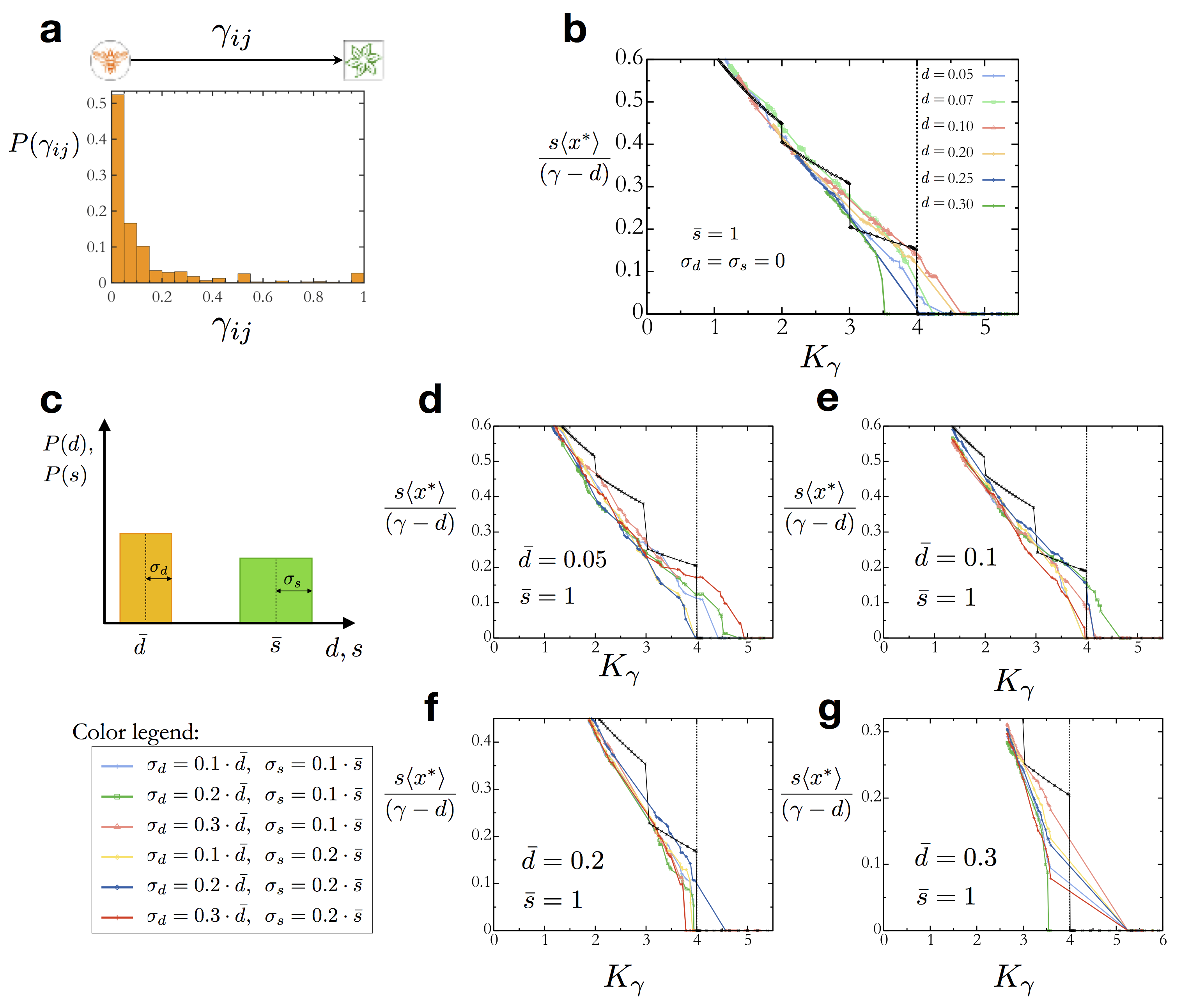
Supplementary Figure 3: Test of the theory. a, Distribution of the interaction strengths for real ecosystems found experimentally and reported in bascompte-linear . The distribution shows a right-skewed shape, which is then used in b, and d-g, to test the theoretical prediction of collapse. b, Rescaled averaged density $\langle x^{*}\rangle$ as a function of $K_{\gamma}$ obtained by numerically integrating Eqs. (1) with $\gamma_{ij}$ sampled from the right-skewed distribution of Supplementary Fig. 3a. The death rate $d$ and the self-limiting parameter $s$ are taken constant and their values are reported in figure. Each curve shows the results of the simulation for a different death rate. The black line illustrates the theoretical solution obtained with the logic approximation for $\bar{d}=0.01$, which lies within in the whole range considered. c, Uniform distribution for the death rates $d_{i}$ and the self-limiting parameters $s_{i}$ which is then used for the simulations shown in the following panels. d-e, Same numerical results as for Supplementary Fig. 3b with death rates and self-limiting parameters no longer constant but i.i.d. and sampled from the distributions shown in c. Mean values are reported in figures. Each curve illustrates the results for a different variance of the distribution $P(d)$ and $P(s)$, as reported in the legend. The black line illustrates the theoretical solution obtained through the logic approximation at the $\bar{d}$-value shown in each panel. The underlying network used for the results presented in Supplementary Fig. 3b, d-g is the same as the one used in Fig. 2 (Net # 10 in Supplementary Table 1).

VI.5 Test of predictions of collapse

To further test our theory, we compare its prediction of the tipping point for the system collapse with the numerical estimation of the same tipping point obtained by integrating Eqs. (1), with the right-skewed $P(\gamma_{ij})$ as in Supplementary Fig. 3a and uniform distribution $P(d_{i})$ and $P(s_{i})$ for the death rate and self-limitation parameters, respectively. We use several different underlying networks of plants-pollinators and plants-seed dispersal from the Interaction Web Database at https://www.nceas.ucsb.edu/interactionweb/. For each of them we iterate Eqs. (1) till the fixed point for different $K_{\gamma}$ values until we reach the point of the system’s collapse, i.e. $\langle x^{*}\rangle=0$, for which $K_{\gamma}=K_{\gamma_{c}}$. Because of the randomness in the interaction strengths, we repeat the process 30 times for each network and the final value of $K_{\gamma_{c}}$ is the average across runs. We then compare this value with the theoretical prediction obtained with the logic approximation, i.e. $K_{\gamma_{c}}=k_{\rm core}^{\rm max}$. Results are shown in Supplementary Fig. 4a where we also report the $R^{2}$-value for the linear fit. From this figure we observe that, as predicted by our theory, the $k_{\rm core}^{\rm max}$ estimates well the point of collapse for the system ($R^{2}=0.89$) and, therefore, it could be used as a predictor of the ecosystem’s extinction.

VI.6 Comparison with other metrics

We next compare our theoretical solution with other metrics that have been used to predict the tipping point. An interesting implication of the k-core is the fact that k-cores are nested, i.e., high k-cores are enclosed in low k-cores (Fig. 1a). According to our solution, the larger the maximum kcore $k_{\rm core}^{\rm max}$ (i.e., the more k-shells in the network) the larger the resilience of the system against external global shocks that reduce the interaction strength $\gamma$. An interesting comparison it is then to study how $k_{\rm core}^{\rm max}$ and nestedness as defined in  bascompte ; olesen correlate with $K_{\gamma_{c}}$. For each of the network considered in SI Section VI.5 we compute the nestedness and plotted it versus the numerical $K_{\gamma_{c}}$. Results are shown in Supplementary Fig. 4b and show that the nestedness correlates weakly with $K_{\gamma_{c}}$ ($R^{2}=0.01$).

We also note that the level of connectance in the network (i.e., the average degree) might be important for the collapse: fully connected networks will collapse abruptly but will have very small $\gamma_{c}$ (high $K_{\gamma_{c}}$), while barely connected ones will collapse for higher values of $\gamma$ (smaller $K_{\gamma}$). It is then interesting to study how well $K_{\gamma_{c}}$ and the connectance correlate with each other. Supplementary Fig. 4c shows significant correlation ($R^{2}=0.56$) between $K_{\gamma_{c}}$ and connectance. Indeed, this is expected since the maximum kcore and maximum degree are related by their bounds $k_{\rm max}\geq k_{\rm core}^{\rm max}$, and the average degree in a given shell is highly correlated with the order of the shell, $k_{s}$, for random networks gallos .

Furthermore, we observe that there are other quantities that are related to the $k_{\rm core}^{\rm max}$ of the network and therefore could be used as proxies of the ecosystem’s collapse. This includes the spectral radius staniczenko and the chromatic number $\chi$ (defined as the smallest number of colors needed to color the vertices of a graph so that no two adjacent vertices share the same color pemmaraju ). This is because the spectral radius is an exact upper bound of the $k_{\rm core}^{\rm max}$ (see Ref. bickle ), and the chromatic number is a lower bound of $k_{\rm core}^{\rm max}$, $\chi\leq k_{\rm core}^{\rm max}+1$ szekeres .

Supplementary Fig. 4d shows the comparison between the spectral radius and the $K_{\gamma_{c}}$ for the same networks examined above and illustrates that also the spectral radius, indeed, correlates well with the tipping point of the system. In Supplementary Fig. 4e-g, whereas, we show how this latter metric as well as the others computed above correlate with the $k_{\rm core}^{\rm max}$. From these results we observe that, those metrics which are well correlated with the tipping point $K_{\gamma_{c}}$, i.e. the spectral radius and the connectance (Supplementary Fig. 4c-d), are also well correlated with our theoretical predictor the $k_{\rm core}^{\rm max}$ (Supplementary Fig. 4e-f), as expected by the fact that the $k_{\rm core}^{\rm max}$ is the theoretical predictor for the tipping point of the ecosystem’s collapse.

In general, all metrics that are related to $k_{\rm core}^{\rm max}$ via mathematical bounds can be approximated predictors of the tipping point. However, since these metrics relate to the $k_{\rm core}^{\rm max}$ only when the bounds are saturated, they may not provide a precise prediction for all type of networks. While, the bounds appear to be saturated in the studied networks, it is not guaranteed that other networks will saturate the bounds as well. Thus, the $k_{\rm core}^{\rm max}$ remains the only metric that can accurately predict the tipping point based on first principles for all types of network architectures. This fact results from the non-perturbative character of our solution which implies that the prediction of the $k_{\rm core}^{\rm max}$ is valid independent of the structure of the network.

VI.7 Other limits of validity

An important condition for the applicability of the k-core solution is that the system must be mutualistic, that is, all the interactions are positive $\gamma_{ij}>0$. The interactions can be directed or undirected, indeed, both cases are solved by different k-cores. However, the condition of positive interactions is crucial to introduce the idea of percolation and k-core, and, without this condition, the k-core percolation cannot be applied to predict the ecosystem’s collapse. For systems where the interactions can have positive and negative strengths, like for instance a predator-prey system, the existence of negative interactions acts as inhibitors in the system and the concept of the k-core as was derived here cannot be applied.

This case, which is out of the scope of the present study, leads to other types of fixed points, e.g. limit cycles, and will be treated in a follow up paper. We anticipate that, while a topological invariant like the k-core is not anymore relevant in this case, other invariants arises that allows to connect the structure of the network to its dynamics.

There exist other effects that are outside the scope of the present study, but, nevertheless, they are important and should be incorporated in future studies. For example, plants are rarely obligate mutualists and engage in a variety of reproductive modes which are neglected in our model. The pollinators in the webs considered here are a subset of those pollinating plants (e.g., beetles are rarely included, but contribute quite a bit to pollination). Furthermore, in our model we have considered that plants do not interact with other plants (nor pollinators with other pollinators). Future work might incorporate these interesting features. The present model could be interpreted as how, other things being equal, the k-core solution may capture the features of the tipping point bascompte-linear . Furthermore, in general, communities of plants and pollinators are under-sampled in datasets, which might contribute to inaccurate predictions bascompte-linear .

VI.8 Changes in death rate

We note that Eq. (7) is symmetric in $\gamma$ and $d$. As a consequence, the collapse also occurs if the death rate $d$ increases beyond the critical value determined by Eq. (7). Changes in $d$ may be due to pollution, habitat destruction, genetic isolation or harvesting, which may be easier to monitor. However, we observe that the effect of variations in $d$ on the critical value $K_{\gamma}$ is much weaker than the effect caused by variations in $\gamma$. Indeed, although that the death rate strongly depends on the life span and can be incredibly different between plants and animals, both the death rates of plants and pollinators are much smaller than the relevant scale of the model which is $\gamma$, in fact $d_{P}\ll d_{A}\ll\gamma$, where subscripts $P$ and $A$ stand for plants and pollinators. For this reason small variation of $d$, have very little or none effect on the integer part of $K_{\gamma}$ since $d\ll\gamma$ and, therefore, variations in $\gamma$ are those which dominates the change in $K_{\gamma}$.

VI.9 Other comparisons

It would be of interest to further test our theoretical prediction based on the k-core using examples of collapsed systems lying in the lower region in Fig. 5a, i.e. below the tipping line. This test would require the reconstruction of a collapsed mutualistic interaction network via fossil records, as has been done for some Cambrian food webs dunne . However, we are not aware of any collapsed mutualistic ecosystems whose interaction network has been compiled using fossil assemblages. Nonetheless, we notice that the tropical network shown in Fig. 5a has larger k-core number than the temperate and arctic networks, thus being more stable, according to our theory. This result suggests higher resilience in tropical networks against extinctions than in temperate or arctic networks, a result that has been noticed in experimental studies specialization . In other words, the theory based on the k-core predicts that the most vulnerable networks have low k-core number, like the arctic and temperate networks in Fig. 5a, and available empirical evidence supports this prediction.

VII Stability of the fixed point solution

The fixed point solution derived in the main text is obtained for the nonlinear system of dynamical Eqs. (1). Such nonlinear dynamical equations are characterized by a sigmoid-like function or Hill function of the interaction term that saturates to a constant for large densities of the interacting species.

The stability of the fixed point solution of the nonlinear dynamical system (1) is controlled by the Jacobian matrix

$$\mathcal{M}_{ij}(\vec{x}^{*})\ =\ \frac{\partial\dot{x}_{i}}{\partial x_{j}}\Bigg{|}_{\vec{x}=\vec{x}^{*}}\ .$$ (49)

More precisely, the fixed point solution $\vec{x}^{*}$ is stable if all eigenvalues of $\hat{\mathcal{M}}$ have a negative real part. The Jacobian (49) for the ecosystem (1) reads:

$$\mathcal{M}_{ij}(\vec{x}^{*})\ =\ -\delta_{ij}\left(d+2sx_{i}^{*}-\gamma\frac{\sum_{k=1}^{N}A_{ik}x_{k}^{*}}{\alpha+\sum_{k=1}^{N}A_{ik}x_{k}^{*}}\right)+\gamma\alpha x_{i}^{*}\frac{A_{ij}}{\left(\alpha+\sum_{k=1}^{N}A_{ik}x_{k}^{*}\right)^{2}}\ ,$$ (50)

where we take for simplicity $\gamma_{ij}=\gamma$. From Supplementary Eqs. (50) we see that the trivial fixed point $\vec{x}^{*}=\vec{0}$ is always stable. In fact, in this case, we find $\mathcal{M}_{ij}(\vec{0})\ =\ -d\delta_{ij}$, and all eigenvalues equal $-d<0$.

As a consequence, the transition from the fixed point $\vec{x}^{*}=\vec{0}$ to the fixed point $\vec{x}^{*}\neq\vec{0}$ cannot be continuous for any finite value of $d>0$, but must be a discontinuous transition. That is, the system must jump from the state $\vec{x}^{*}\neq\vec{0}$ to the state $\vec{x}^{*}\neq\vec{0}$.

At the nontrivial fixed point, the Jacobian evaluates:

$$\mathcal{M}_{ij}(\vec{x}^{*})\ =\ -sx_{i}^{*}\ \Theta(x_{i}^{*})\left[\delta_{ij}-\frac{\gamma\alpha}{s}\frac{A_{ij}}{\left(\alpha+\sum_{k=1}^{N}A_{ik}x_{k}^{*}\right)^{2}}\right]\ ,$$ (51)

where the Heaviside (Theta) function $\Theta(x_{i}^{*})$ indicates that $\mathcal{M}_{ij}$ must be restricted to the extant species, i.e., the ones such that $x_{i}^{*}>0$. Next, we use the reduced density $y_{i}^{*}=\frac{s}{\gamma-d}\sum_{j=1}^{N}A_{ij}x_{j}^{*}$, and Supplementary Eqs. (51) as

$$\mathcal{M}_{ij}(\vec{x}^{*})\ =\ -sx_{i}^{*}\ \Theta(x_{i}^{*})\left[\delta_{ij}-\frac{\gamma\alpha}{s}\frac{A_{ij}}{\left(\alpha+\frac{\gamma-d}{s}y_{i}^{*}\right)^{2}}\right]\ ,$$ (52)

To simplify both notation and interpretation of the subsequent results, we notice that, for small $d$, the threshold $K_{\gamma}$ equals $K_{\gamma}=\alpha s/\gamma+O(d)$. Then, taking only the leading order in $d$, we can write $\hat{\mathcal{M}}$ as:

$$\mathcal{M}_{ij}(\vec{x}^{*})\ =\ -sx_{i}^{*}\ \Theta(x_{i}^{*})\left[\delta_{ij}-A_{ij}\frac{K_{\gamma}}{(K_{\gamma}+y_{i}^{*})^{2}}\right]\ .$$ (53)

Using Supplementary Eqs. (34) (at the leading order in $d$) to express $x_{i}^{*}$ in terms of $y_{i}^{*}$, we finally obtain $\hat{\mathcal{M}}$ as a function of $\vec{y}^{*}$:

$$\mathcal{M}_{ij}(\vec{y}^{*})\ =\ -\gamma\frac{y_{i}^{*}}{K_{\gamma}+y_{i}^{*}}\ \Theta(y_{i}^{*})\left[\delta_{ij}-A_{ij}\frac{K_{\gamma}}{(K_{\gamma}+y_{i}^{*})^{2}}\right]\ ,$$ (54)

which we can rewrite using the Hill function notation as:

$$\mathcal{M}_{ij}(\vec{y}^{*})\ =\ -\gamma H_{1}(y_{i}^{*},K_{\gamma})\ \Theta(y_{i}^{*})\left[\delta_{ij}-A_{ij}\frac{H_{1}(K_{\gamma},y_{i}^{*})}{K_{\gamma}+y_{i}^{*}}\right]\ .$$ (55)

At this point we use the logic approximation of the Hill functions. Noticing that

$$H_{1}(y_{i}^{*},K_{\gamma})H_{1}(K_{\gamma},y_{i}^{*})\approx\Theta(y_{i}^{*}-K_{\gamma})\Theta(K_{\gamma}-y_{i}^{*})=0\ ,$$ (56)

Supplementary Eqs. (55) becomes

$$\mathcal{M}_{ij}(\vec{y}^{*})\ =\ -\gamma H_{1}(y_{i}^{*},K_{\gamma})\ \Theta(y_{i}^{*})\delta_{ij}\ .$$ (57)

The eigenvalues of $\hat{\mathcal{M}}(\vec{y}^{*})$ can be read directly from Supplementary Eqs. (57), and are given by:

$$\lambda^{\mathcal{M}}_{i}=-\gamma\frac{\mathcal{N}_{i}(K_{\gamma})}{K_{\gamma}+\mathcal{N}_{i}(K_{\gamma})}\Theta[\mathcal{N}_{i}(K_{\gamma})]\ ,\ \ \ \ \ i=1\dots,N\ ,$$ (58)

which are Eqs. (8) presented in the main text. The largest eigenvalue is

$$\lambda^{\mathcal{M}}_{\rm max}=\max_{i}\lambda^{\mathcal{M}}_{i}\ .$$ (59)

The condition for stability of the feasible solution is then

$$\lambda^{\mathcal{M}}_{\rm max}<0\ ,$$ (60)

which guarantees that all other eigenvalues are negative and therefore the stability of the feasible solution.

According to (58), the largest eigenvalue is attained by the species with the least number of connections to the $K_{\gamma}$-core. Notice that each eigenvalue is associated with a single species. The worst case scenario is a commensalist with just one link to the $K_{\gamma}$-core (for instance the commensalists # 1 and # 8 depicted in Fig. 3c) so that the upper bound of the largest eigenvalue is

$$\lambda^{\mathcal{M}}_{\rm max}=-\frac{\gamma}{K_{\gamma}+1}\ ,$$ (61)

which is always negative. Therefore, the nontrivial feasible solution $y_{i}^{*}$ is always stable, as long as this nonzero solution exists.

On the other hand, when $K_{\gamma}>k_{\rm core}^{\rm max}$, all $\mathcal{N}_{i}$ vanish, i.e. $\mathcal{N}_{i}(K_{\gamma}>k_{\rm core}^{\rm max})=0$. Simultaneously, all the eigenvalues become zero, $\lambda^{\mathcal{M}}_{i}=0$, signaling the simultaneous onset of collapse and instability of the nonzero fixed point solution. In fact, we have discussed after Eqs. (6) that the solution becomes unfeasible and the system must collapse when $K_{\gamma}=k_{\rm core}^{\rm max}$. Thus, we recover from the stability analysis the tipping point Eq. (7), which we obtained in the main text by requiring the feasibility of the nontrivial fixed point solution. That is, we find that the feasible nontrivial nonzero fixed point solution becomes unstable, $\lambda^{\mathcal{M}}_{\rm max}=0$, at the same time that it becomes unfeasible, $K_{\gamma}=k_{\rm core}^{\rm max}$.

VII.1 Stability analysis of Ref. may3

Having discussed the stability of our fixed point solution, we discuss next a method frequently used in the literature to study the stability of ecosystems modeled as dynamical systems for which the solution to the fixed point equations is not known may3 . This method ignores the dependence of the stability matrix $\hat{\mathcal{M}}$ from the fixed point solution, and considers, instead, the alternative stability matrix $\hat{\mathcal{M^{\prime}}}$ may3 :

$$\mathcal{M}^{\prime}_{ij}\ =\ -\delta_{ij}+\frac{A_{ij}}{K_{\gamma}}\ .$$ (62)

Here the adjacency matrix $A_{ij}$ is modeled as a random matrix, giving rise to a random stability matrix $\mathcal{M}^{\prime}_{ij}$ and therefore this method is inspired by Wigner semi-circle law of random matrices.

The stability condition is again that all eigenvalues of $\mathcal{M}^{\prime}_{ij}$ have negative real parts. In this case this stability condition is expressed by the following:

$$\lambda^{A}_{\rm max}<K_{\gamma}\,\,\,\,\,\mbox{(condition of stability in Ref.~{}\cite[cite]{\@@bibref{Authors Phrase1YearPhrase2}{may3}{\@@citephrase{(}}{\@@citephrase{)}}}),}$$ (63)

where $\lambda^{A}_{\rm max}$ is the largest eigenvalue of the adjacency matrix $\hat{A}$. This approximation leads to the so-called diversity-stability paradox may3 , according to which increasing the number of different mutualistic species will eventually destabilize the ecosystem. This happens because the largest eigenvalue $\lambda^{A}_{\rm max}$ of the matrix $\hat{\mathcal{M^{\prime}}}$ in Supplementary Eqs. (62) is a nondecreasing function of the number of different species, and thus the condition $\lambda^{A}_{\rm max}<K_{\gamma}$ can be hardly satisfied for a large diverse ecosystem. The diversity-stability paradox for mutualistic ecosystem is, however, a by-product of the approximative method leading to the stability matrix (62) which ignores the actual contribution of the fixed point solution to the stability condition.

Indeed, the exact stability analysis leading to Supplementary Eqs. (58), by taking into account the dependence of the stability matrix from the fixed point solution, does not contain the diversity-stability paradox. On the contrary, it points to the opposite conclusion that diversity of symbionts increases the robustness of mutualistic ecosystems. Specifically, increasing the number of symbionts who are located in the maximum k-core of the network will eventually increase the k-core number $k_{\rm core}^{\rm max}$ of their network. As a consequence the stability condition Eq. (9): $K_{\gamma}<k_{\rm core}^{\rm max}$ will be easier and easier to satisfy as diversity of symbionts increases. Similarly, mutualistic cooperation stabilizes the system since it leads to smaller $K_{\gamma}$ and, again, Eq. (9) is easier and easier to satisfy as the mutualistic interactions get stronger. In conclusion, the stability of mutualistic ecosystem is primarily controlled by the k-core organization of the underlying interaction network according to Eq. (9), where the diversity-stability paradox disappears and mutualistic interactions are beneficial for the robustness of the ecosystem.

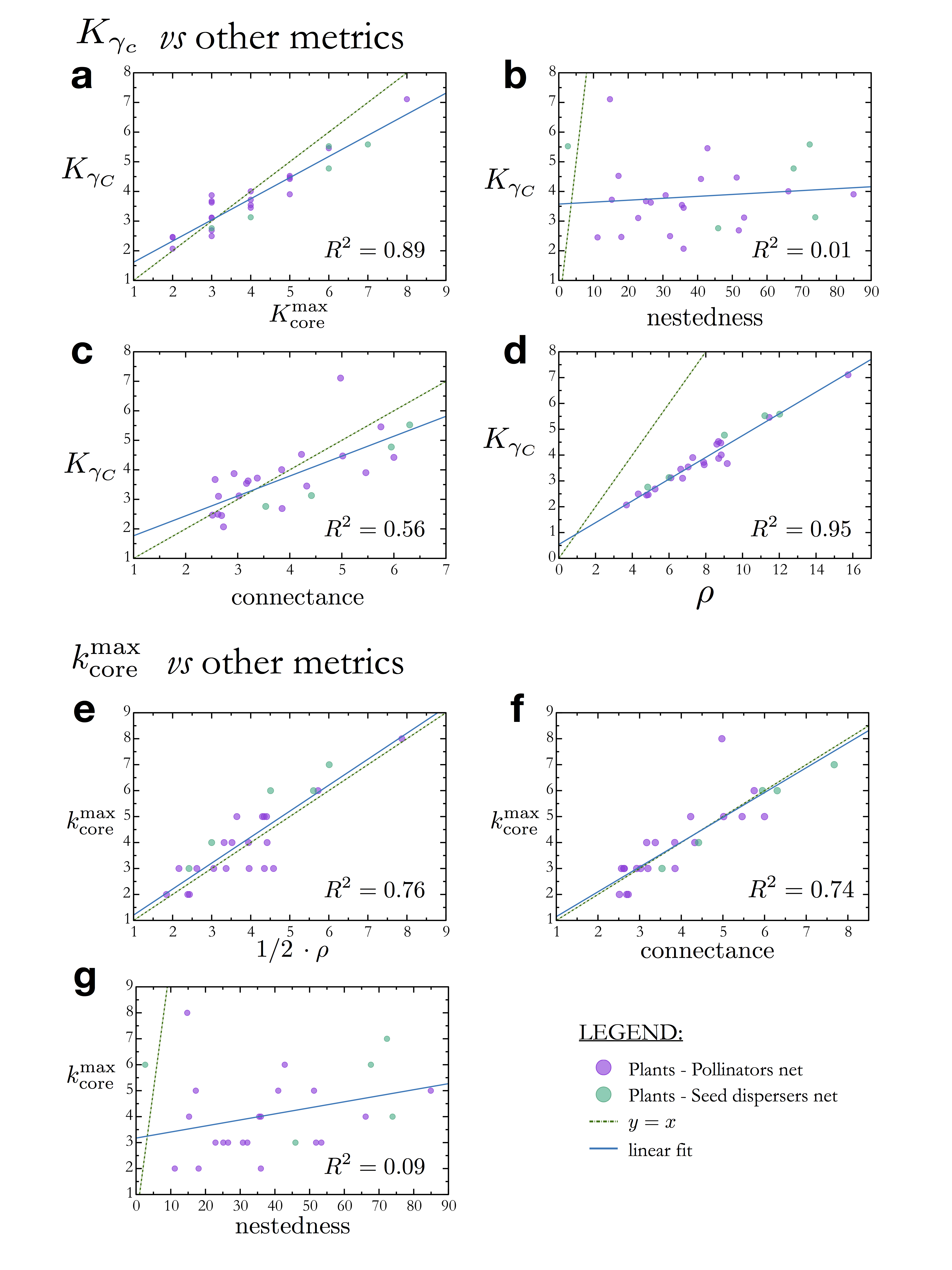
Supplementary Figure 4: Caption in the next page.

Supplementary Figure 4: Comparison with other metrics. a-d Comparison between the $K_{\gamma_{c}}$ value at the tipping point of collapse of the system and different metrics, for different networks of plants-pollinators and plants-seed dispersals from the Interaction Web Database at https://www.nceas.ucsb.edu/interactionweb/. In each plot, each point represents the result of the tipping point vs a given metric for a specific network. In each panel, $K_{\gamma_{c}}$ is compared with: a, the $K_{\rm core}^{\rm max}$, b, the nestedness bascompte ; olesen , c, the connectance (defined as the average number of node’s connection in the network), d, and the spectral radius staniczenko . The critical value $K_{\gamma_{c}}$ for the tipping point of the system is obtained by numerically integrating Eqs. (1) with $P(\gamma_{ij})$ as in Supplementary Fig. 3a till the fixed point and by changing the value of $K_{\gamma}$ till one finds the point at which all the species go extinct, i.e. $\langle x^{*}\rangle$, (at that point $K_{\gamma}$ = $K_{\gamma_{c}}$). To vary the value of $K_{\gamma}$, we change the average $\gamma$ in the $P(\gamma_{ij})$ by shifting the minimal $\gamma$-value of the distribution weights accordingly. e-g Comparison between our theoretical predictor for the tipping point of collapse of the system, i.e. the $K_{\rm core}^{\rm max}$, and other metrics used to characterize ecological networks: e, the spectral radius, f, the connectance, g, the nestedness. In each panel we plot the line $y=x$ and also the line corresponding to a linear fit of the data. R-squared values are reported for each figure inside the plot frame. Overall, results show that the $k_{\rm{core}}^{\rm max}$ correlates well with $K_{\gamma_{c}}$ and that those metrics which correlate well with the $k_{\rm{core}}^{\rm max}$, as the connectance and the spectral radius (panel c and d respectively), also correlate with $K_{\gamma_{c}}$ (see panel e and f). The $k_{\rm{core}}^{\rm max}$ and the spectral radius are mathematically related, indeed the spectral radius is always an upper bound of the $k_{\rm{core}}^{\rm max}$ bickle .

References

- (1) May, R. M. Will a large complex system be stable? Nature 238, 413-414 (1972).
- (2) Strogatz, S. Nonlinear dynamics and chaos: with applications to physics, biology, chemistry, and engineering (Westview Press, 2000).
- (3) Caldarelli, G. & Vespignani, A. Large Scale Structure and Dynamics of Complex Networks: From Information Technology to Finance and Natural Science (World Scientific, Singapore, 2007).
- (4) Buldyrev, S. V., Parshani, R., Paul, G., Stanley, H. E. & Havlin, S. Catastrophic cascade of failures in interdependent networks. Nature 464, 1025-1028 (2010).
- (5) Scheffer, M. et al. Early-warning signals for critical transitions. Nature 461, 53-59 (2009).
- (6) Scheffer, M. et al. Anticipating critical transitions. Science 338, 344-348 (2012).
- (7) Allesina, S. & Tang, S. Stability criteria for complex ecosystems. Nature 483, 205-208 (2012).
- (8) Gao, J., Barzel, B. & Barabási, A.-L. Universal resilience patterns in complex networks. Nature 530, 307-312 (2016).
- (9) Bascompte, J., Jordano, P. & Olesen, J. M. Asymmetric coevolutionary networks facilitate biodiversity maintenance. Science 312, 431-433 (2006).
- (10) Coyte, K. Z., Schluter, J. & Foster, K. R. The ecology of the microbiome: Networks, competition, and stability. Science 350, 663-666 (2015).
- (11) Haldane, A. G. & May, R. M. Systemic risk in banking ecosystems. Nature 469, 351-355 (2011).
- (12) Battiston, S., Caldarelli, G., Georg, C.-P., May, R. M. & Stiglitz, J. Complex derivatives. Nat. Phys. 9, 123-125 (2013).
- (13) Dai, L., Vorselen, D., Korolev, K. S. & Gore, J. Generic indicators for loss of resilience before a tipping point leading to population collapse. Science 336, 1175-1177 (2012).
- (14) Seidman, S. B. Network structure and minimum degree. Soc. Networks 5, 269-287 (1983).
- (15) Pittel, B., Spencer, J. & Wormald, N. Sudden emergence of a giant k-core in a random graph. J. Comb. Theory, Series B 67, 111-151 (1996).
- (16) Dorogovtsev, S. N., Goltsev, A. V. & Mendes, J. F. F. k-core organization of complex networks. Phys. Rev. Lett. 96, 040601 (2006).
- (17) Carmi, S., Havlin, S., Kirkpatrick, S., Shavitt, Y. & Shir, E. A model of Internet topology using k-shell decomposition. Proc. Natl. Acad. Sci. U.S.A. 104, 11150-11154 (2007).
- (18) Alvarez-Hamelin, J. I., Dall’Asta, L., Barrat, A. & Vespignani, A. k-core decomposition of the internet graphs: hierarchies, self-similarity and measurement biases. Netw. Heterog. Media 3, 371 (2008).
- (19) Kitsak, M., Gallos, L. K., Havlin, S., Liljeros, F., Muchnik, L., Stanley, H. E. & Makse, H. A. Identification of influential spreaders in complex networks. Nat. Phys. 6, 888-893 (2010).
- (20) Hagmann, P., Cammoun, L., Gigandet, X., Meuli, R., Honey, C. J., Wedeen, V. J. & Sporns, O. Mapping the structural core of human cerebral cortex. Plos Biol. 6, e159 (2008).
- (21) Morone, F., Burleson-Lesser, K., Vinutha, H. A., Sastry, S. & Makse, H. A. The jamming transition is a k-core percolation transition, arXiv:1804.07804 (2018).
- (22) May, R. M. Mutualistic interactions among species. Nature 296, 803-804 (1982).
- (23) Holland, J. N., DeAngelis, D. L. & Bronstein, J. L. Population dynamics and mutualism: functional responses of benefits and costs. Am. Nat. 159, 231-244 (2002).
- (24) Bastolla, U., Fortuna, M. A., Pascual-García, A., Ferrera, A., Luque, B. & Bascompte, J. The architecture of mutualistic networks minimizes competition and increases biodiversity. Nature 458, 1018-1020 (2009).
- (25) Thebault, E. & Fontaine, C. Stability of ecological communities and the architecture of mutualistic and trophic networks. Science 329, 853-856 (2010).
- (26) Alon, U. An Introduction to Systems Biology: Design Principles of Biological Circuits (CRC Press, 2006).
- (27) Amit, D. J. Modeling Brain Function: The World of Attractor Neural Networks (Cambridge University Press, 1989).
- (28) Sompolinsky, H., Crisanti, A. & Sommers, H. J. Chaos in random neural networks. Phys. Rev. Lett. 61, 259-262 (1988).
- (29) Okuyama, T. & Holland, J. N. Network structural properties mediate the stability of mutualistic communities. Ecol. Lett. 11, 208-216 (2008).
- (30) Arroyo, M. T. K., Primack, R. B. & Armesto, J. J. Community studies in pollination ecology in the high temperate Andes of Central Chile. I. Pollination mechanisms and altitudinal variation. Amer. J. Bot. 69, 82-97 (1982).
- (31) May, R. M. Simple mathematical models with very complicated dynamics. Nature 261, 459-467 (1976).
- (32) Shen-Orr, S. S., Milo, R., Mangan, S. & Alon, U. Network motifs in the transcriptional regulation net- work of Escherichia coli. Nature Genet. 31, 64-68 (2002).
- (33) Kauffman, S. A. The Origins of Order: Self-organization and Selection in Evolution (Oxford University Press, New York, 1993).
- (34) Glass, L. & Kauffman, S. A. The logical analysis of continuous, non-linear biochemical control networks. J. Theor. Biol. 38, 103-129 (1973).
- (35) Rohr, R. P., Saavedra, S. & Bascompte, J. On the structural stability of mutualistic systems. Science 345, 1253497 (2014).
- (36) Bascompte, J., Jordano, P., Melián, C. J. & Olesen, J. M. The nested assembly of plant-animal mutualistic networks, Proc. Natl. Acad. Sci. U.S.A. 100, 9383-9387 (2003).
- (37) Staniczenko, P. P. A., Kopp, J. C. & Allesina, S. The ghost of nestedness in ecological networks. Nat. Commun. 4, 1931 (2013).
- (38) Bickle, A. Cores and shells of graphs. Mathematica Bohemica 138, 43-59 (2013).
- (39) Berry, D. & Widder, S. Deciphering microbial interactions and detecting keystone species with co-occurrence networks. Front Microbiol. 5, 1-14 (2014).
- (40) Morone, F. & Makse, H. A. Influence maximization in complex networks through optimal percolation. Nature 524, 65-68 (2015).
- (41) Bucci, V., Bradde, S., Biroli, G. & Xavier, J. B. Social interaction, noise and antibiotic-mediated switches in the intestinal microbiota. Plos Comput. Biol. 8, e1002497 (2012).
- (42) Kato, M., Makutani, T., Inoue, T., Itino, T. Insect-flower relationship in the primary beech forest of Ashu, Kyoto: an overview of the flowering phenology and seasonal pattern of insect visits. Contr. Biol. Lab. Kyoto Univ. 27, 309-375 (1990).

References

- (1) Dakos, V. & Bascompte, J. Critical slowing down as early warning for the onset of collapse in mutualistic communities. Proc. Natl. Acad. Sci. U.S.A. 111, 17546-17551 (2014).
- (2) Szekeres, G. & Wilf, H.S. An inequality for the chromatic number of a graph. J. Comb. Theory 4, 1-3 (1968).
- (3) Tyson, J. J., Chen, K. C. & Novak, B. Sniffers, buzzers, toggles and blinkers: dynamics of regulatory and signaling pathways in the cell. Curr. Opin. Cell. Biol. 15, 221-231 (2003).
- (4) Karlebach, G. and Shamir, R. Modelling and analysis of gene regulatory networks. Nat. Rev. Mol. Cell Biol. 9, 770-780 (2008).
- (5) Okuyama, T. & Holland, J. N. Network structural properties mediate the stability of mutualistic communities. Ecol. Lett. 11, 208-216 (2008).
- (6) B. Beehler, Frugivory and polygamy in birds of paradise. Auk 100, 1-12 (1983).
- (7) Inouye, D. W., Pyke, G. H. Pollination biology in the Snowy Mountains of Australia: comparisons with montane Colorado, USA. Aust. J. Ecol. 13, 191-210 (1988).
- (8) Elberling, H., Olesen, J. M. The structure of a high latitude plant-flower visitor system: the dominance of flies. Ecography 22, 314-323 (1999).
- (9) Mosquin, T., Martin, J. E. H. Observations on the pollination biology of plants on Melville Island, N.W.T., Canada. Can. Field Nat. 81, 201-205 (1967).
- (10) Olesen, J. M., Eskildsen, L. I., Venkatasamy, S. Invasion of pollination networks on oceanic islands: importance of invader complexes and endemic super generalists. Divers. Distrib. 8, 181-192 (2002).
- (11) Schemske, D. W. et al. Flowering Ecology of Some Spring Woodland Herbs. Ecology 59, 351-366 (1978).
- (12) Hocking, B. Insect-flower associations in the high Arctic with special reference to nectar. Oikos 19, 359-388 (1968).
- (13) Sorensen, A.E. Interactions between birds and fruit in a temperate woodland. Oecologia 50, 242-249 (1981).
- (14) Pemmaraju, S., & Skiena, S. Computational Discrete Mathematics: Combinatorics and Graph Theory with Mathematica (Cambridge university press, 2003).
- (15) Dunne, J. A., Williams, R. J., Martinez, N. D., Wood, R. A. & Erwin, D. H. Compilation and network analysis of Cambrian food webs. PLoS Biol. 6, e102 (2008).
- (16) Schleuning, M., et al. Specialization of mutualistic interaction networks decreases toward tropical latitudes. Current Biology 22, 1925-1931 (2012).