Bertsimas and Cory-Wright

A Scalable Algorithm For Sparse Portfolio Selection

A Scalable Algorithm for Sparse Portfolio Selection

Dimitris Bertsimas Sloan School of Management, Massachusetts Institute of Technology, Cambridge, MA, USA.
ORCID: $0000$-$0002$-$1985$-$1003$
dbertsim@mit.edu Ryan Cory-Wright Operations Research Center, Massachusetts Institute of Technology, Cambridge, MA, USA,
ORCID: $0000$-$0002$-$4485$-$0619$
ryancw@mit.edu

The sparse portfolio selection problem is one of the most famous and frequently-studied problems in the optimization and financial economics literatures. In a universe of risky assets, the goal is to construct a portfolio with maximal expected return and minimum variance, subject to an upper bound on the number of positions, linear inequalities and minimum investment constraints. Existing certifiably optimal approaches to this problem have not been shown to converge within a practical amount of time at real-world problem sizes with more than $400$ securities. In this paper, we propose a more scalable approach. By imposing a ridge regularization term, we reformulate the problem as a convex binary optimization problem, which is solvable via an efficient outer-approximation procedure. We propose various techniques for improving the performance of the procedure, including a heuristic which supplies high-quality warm-starts, and a second heuristic for generating additional cuts which strengthens the root relaxation. We also study the problem’s continuous relaxation, establish that it is second-order-cone representable, and supply a sufficient condition for its tightness. In numerical experiments, we establish that a conjunction of the imposition of ridge regularization and the use of the outer-approximation procedure gives rise to dramatic speedups for sparse portfolio selection problems.

Sparse Portfolio Selection, Binary Convex Optimization, Outer Approximation. This paper was first submitted in November $2020$. A revision was submitted in March $2021$. programming: integer; non-linear: quadratic; finance: portfolio

Design and Analysis of Algorithms-Discrete

1 Introduction

Since the Nobel-prize winning work of Markowitz (1952), the problem of selecting an optimal portfolio of securities has received an enormous amount of attention from practitioners and academics alike. In a universe containing $n$ distinct securities with expected marginal returns $\bm{\mu}\in\mathbb{R}^{n}$ and a variance-covariance matrix of the returns ${\bm{\Sigma}\in S^{n}_{+}}$, the scalarized Markowitz model selects a portfolio which provides the highest expected return for a given amount of variance, by solving:

$$\min_{\bm{x}\in\mathbb{R}^{n}_{+}}\ \frac{\sigma}{2}\bm{x}^{\top}\bm{\Sigma}\bm{x}-\bm{\mu}^{\top}\bm{x}\quad\text{s.t.}\quad\bm{e}^{\top}\bm{x}=1,$$ (1)

where $\sigma\geq 0$ is a parameter that controls the trade-off between the portfolios risk and return, and $\bm{e}\in\mathbb{R}^{n}$ denotes the vector of all ones.

To improve its realism, many authors have proposed augmenting Problem (1) with minimum investment, maximum investment, and cardinality constraints among others (see, e.g., Jacob 1974, Perold 1984, Chang et al. 2000). Unfortunately, these constraints are disparate and sometimes imply each other, which makes defining a canonical portfolio selection model challenging. We refer to Mencarelli and D’Ambrosio (2019) for a survey of real-life portfolio selection constraints.

Bienstock (1996) (see also Bertsimas et al. 1999) defined a realistic portfolio selection model by augmenting Problem (1) with two sets of inequalities. The first set is a generic system of linear inequalites $\bm{l}\leq\bm{A}\bm{x}\leq\bm{u}$ which, through an appropriate choice of data $\bm{l}\in\mathbb{R}^{m},\bm{u}\in\mathbb{R}^{m},\bm{A}\in\mathbb{R}^{m\times n}$, ensures that various real-world constraints such as allocating an appropriate amount of capital to each market sector hold. The second inequality limits the number of non-zero positions held to $k\ll n$, by requiring that the portfolio is $k$-sparse, i.e., $\|\bm{x}\|_{0}\leq k$. The sparsity constraint is important because (a) managers incur monitoring costs for each non-zero position, and (b) investors believe that portfolio managers who do not control the number of positions held perform index-tracking while charging active management fees (see Bertsimas et al. 1999, for an implementation of portfolio selection with sparsity constraints at a real-world asset management company); see also (Bertsimas and Weismantel 2005, Chap. 11.1) for further discussion on the motivation for setting $k\ll n$. Imposing the real-world constraints yields the following portfolio selection model:

$$\min_{\bm{x}\in\mathbb{R}^{n}_{+}}\ \frac{\sigma}{2}\bm{x}^{\top}\bm{\Sigma}\bm{x}-\bm{\mu}^{\top}\bm{x}\quad\text{s.t.}\quad\bm{l}\leq\bm{A}\bm{x}\leq\bm{u},\ \bm{e}^{\top}\bm{x}=1,\ \|\bm{x}\|_{0}\leq k.$$ (2)

Note that Problem (2) is NP-hard—even in the absence of linear inequalities (Gao and Li 2013).

By introducing binary variables $z_{i}$ which model whether $x_{i}$ takes non-zero values by requiring that $x_{i}=0$ if $z_{i}=0$, we rewrite the above problem as a convex mixed-integer quadratic problem:

$$\min_{\bm{z}\in\{0,1\}^{n}:\bm{e}^{\top}\bm{z}\leq k,\ \bm{x}\in\mathbb{R}^{n}_{+}}\ \frac{\sigma}{2}\bm{x}^{\top}\bm{\Sigma}\bm{x}-\bm{\mu}^{\top}\bm{x}\quad\text{s.t.}\quad\bm{l}\leq\bm{A}\bm{x}\leq\bm{u},\ \bm{e}^{\top}\bm{x}=1,\ x_{i}=0\ \text{if}\ z_{i}=0\quad\forall i\in[n].$$ (3)

In the past $20$ years, a number of authors have proposed approaches for solving Problem (2) to certifiable optimality. However, no method has been shown to scale to real-world problem sizes where $500\leq n\leq 3,200$ and $k\ll n$. This lack of scalability presents a challenge for practitioners and academics alike, because a scalable algorithm for Problem (2) has numerous financial applications, while algorithms which do not scale to this problem size are less practically useful.

1.1 Problem Formulation and Main Contributions

In this paper, we provide two main contributions. Our first contribution is augmenting Problem (2) with a ridge regularization term, namely $1/(2\gamma)\cdot\|\bm{x}\|_{2}^{2}$—where $\gamma>0$ is fixed—to yield:

$$\min_{\bm{x}\in\mathbb{R}^{n}_{+}}\ \frac{\sigma}{2}\bm{x}^{\top}\bm{\Sigma}\bm{x}+\frac{1}{2\gamma}\|\bm{x}\|_{2}^{2}-\bm{\mu}^{\top}\bm{x}\quad\text{s.t.}\quad\bm{l}\leq\bm{A}\bm{x}\leq\bm{u},\ \bm{e}^{\top}\bm{x}=1,\ \|\bm{x}\|_{0}\leq k.$$ (4)

This problem is more practically tractable than Problem (2), for two reasons. First, as we formally establish in Section 4.2, the duality gap between Problem (4) and its second-order cone relaxation decreases as we decrease $\gamma$ and becomes $0$ at some finite $\gamma>0$. Second, as we numerically establish in Section 5, the algorithms developed here converge more rapidly when $\gamma$ is smaller.

In addition to being more practically tractable, Problem (4) is a computationally useful surrogate for Problem (2). Indeed, as we formally establish in Section 3.4, any optimal solution to Problem (4) is a $1/(2\gamma)$-optimal solution to Problem (2). Moreover, one can find a solution to Problem (2) which is—often substantially—better than this, by (a) solving Problem (4) and (b) solving a simple quadratic optimization problem over the set of securities with the same support as Problem (4)’s solution and an unregularized objective. Indeed, since there are finitely many $k$-sparse binary support vectors, this strategy recovers an optimal solution to (2) for any sufficiently large $\gamma$.

Our second main contribution is a scalable outer-approximation algorithm for Problem (4). By utilizing Problem (4)’s regularization term, we question the modeling paradigm of writing the logical constraint “$x_{i}=0$ if $z_{i}=0$” as $x_{i}\leq z_{i}$ in Problem (4), by substituting the equivalent but non-convex term $x_{i}z_{i}$ for $x_{i}$ and invoking strong duality and that $z_{i}^{2}=z_{i}$ to obtain a convex mixed-integer quadratic reformulation of the problem. This allows us to propose a new outer-approximation algorithm in the spirit of the methods of Duran and Grossmann (1986), Fletcher and Leyffer (1994) but applied to a perspective reformulation (Frangioni and Gentile 2006, Günlük and Linderoth 2012) of the problem which solves large-scale sparse portfolio selection problems with up to $3,200$ securities to certifiable optimality in $100$s or $1000$s of seconds.

1.1.1 Connection Between Regularization and Robustness:  

While we have introduced ridge regularization as a device which improves the problems tractability while only marginally affecting the optimal objective value, one can actually interpret the regularizer as a robustification technique which improves the overall quality of the selected portfolio. Indeed, Ledoit and Wolf (2004) (see also Carrasco and Noumon 2011) have demonstrated that, in mean-variance portfolio selection problems, the largest eigenvalues of the sample covariance matrix $\bm{\Sigma}$ are systematically biased upwards and the smallest eigenvalues of $\bm{\Sigma}$ are systematically biased downwards. As a result, imposing a ridge regularization term (with a properly cross-validated $\gamma$) leads to portfolios which perform better out-of-sample. In a similar vein, DeMiguel et al. (2009) has shown that the strategy of allocating an identical amount of capital to each security outperforms $13$ other popular investment strategies. Since a ridge regularization term encourages investing a more equal amount in each security, DeMiguel et al. (2009)’s work suggests that a ridge regularization term is beneficial.

1.2 The Scalability of State-of-the-Art Approaches

We now review the scalability of existing state-of-the-art approaches, as stated by their authors, in order to justify our claim that no existing method has been shown to scale to problem sizes where ${500\leq n\leq 3,200}$ and ${20\leq k\leq 50}$. In this direction, Table 1 depicts the largest problem solved by each approach, as reported by its authors, and Table 2 depicts the constraints imposed.

We remark that, as indicated in Table 2, each of the existing approaches was benchmarked on a different data set using a different solver and a different processor, which makes Table 1 an imperfect comparison with our method. Nonetheless, Table 1 appears to be about as accurate a comparison as we can reasonably hope to achieve within the scope of this work. Indeed, a more accurate comparison would require re-implementing these methods from scratch and benchmarking them using the same machine/solver, which, as we are not aware of publicly available source code for any of these methods other than Vielma et al. (2017), would require a separate review paper.

Table 1: Largest portfolio instance solved during benchmarking, by approach. “$k_{\max}$” denotes the largest cardinality-constraint right-hand-side imposed when benchmarking. “n/a” indicates that a cardinality constraint was not imposed. “SDO” denotes a method which involves solving an auxiliary semidefinite optimization problem.

Reference	Solution method	Largest instance solved	$k_{\max}$
		(no. securities)
Vielma et al. (2008)	Nonlinear Branch-and-Bound	$100$	$10$
Bonami and Lejeune (2009)	Nonlinear Branch-and-Bound	$200$	n/a
Frangioni and Gentile (2009)	Branch-and-Cut+SDO	$400$	n/a
Gao and Li (2013)	Nonlinear Branch-and-Bound	$300$	$20$
Cui et al. (2013)	Nonlinear Branch-and-Bound	$300$	$10$
Zheng et al. (2014)	Branch-and-Cut+SDO	$400$	$12$
Frangioni et al. (2016)	Branch-and-Cut+SDO	$400$	$10$
Vielma et al. (2017)	Branch-and-Bound	$200$	$10$
Frangioni et al. (2017)	Branch-and-Cut+SDO	$400$	$10$

Table 2: Constraints imposed and solver used, by reference; see also (Mencarelli and D’Ambrosio 2019, Table 1). We use the following notation to refer to the constraints imposed: C: A Cardinality constraint $\|\bm{x}\|_{0}\leq k$; MR: A Minimum Return constraint $\bm{\mu}^{\top}\bm{x}\geq\bar{r}$; SC: A Semi-Continuous, or minimum investment, constraint $x_{i}\in\{0\}\cup[l_{i},u_{i}]\ \forall i\in[n]$; SOC: A Second-Order-Cone approximation of a chance constraint: $\bm{\mu}^{\top}\bm{x}+F^{-1}_{\bm{x}}(1-p)\sqrt{\bm{x}^{\top}\bm{\Sigma}\bm{x}}\geq R$; LS: A Lot-sizing constraint $x_{i}=M\rho_{i}:\rho_{i}\in\mathbb{Z}$.

Reference	Solver		C	MR	SC	SOC	LS	Data Source
Vielma et al. (2008)	CPLEX $10.0$		✓	✗	✗	✓	✗	$20$ instances generated
								using S$\&$P $500$ daily returns
Bonami and Lejeune (2009)	CPLEX $10.1$,		✗	✗	✓	✓	✓	$36$ instances generated
	Bonmin							using S$\&$P $500$ daily returns
Frangioni and Gentile (2009)	CPLEX $11$		✗	✓	✓	✗	✗	Frangioni and Gentile (2006)
Cui et al. (2013)	CPLEX $12.1$		✓	✓	✓	✗	✗	$20$ self-generated instances
Gao and Li (2013)	CPLEX $12.3$,		✓	✓	✗	✗	✗	$58$ instances generated
	MOSEK							using S$\&$P $500$ daily returns
Zheng et al. (2014)	CPLEX $12.4$		✓	✓	✓	✗	✗	Frangioni and Gentile (2006)
								OR-library (Beasley 1990)
Frangioni et al. (2016)	CPLEX $12.6$		✓	✓	✓	✗	✗	Frangioni and Gentile (2006)
Vielma et al. (2017)	CPLEX $12.6$,		✓	✗	✗	✓	✗	$200$ instances generated by
	Gurobi $5.6$							Vielma et al. (2008)
Frangioni et al. (2017)	CPLEX $12.7$		✓	✓	✓	✗	✗	Frangioni and Gentile (2006)
This paper	CPLEX $12.8$		✓	✓	✓	✗	✗	Frangioni and Gentile (2006)
	MOSEK							OR-library Beasley (1990)

1.3 Background and Literature Review

Our work touches on three different strands of the mixed-integer non-linear optimization literature, each of which propose certifiably optimal methods for solving Problem (2): (a) branch-and-bound methods which solve a sequence of relaxations, (b) decomposition methods which separate the discrete and continuous variables in Problem (2), and (c) perspective reformulation methods which obtain tight relaxations by linking the discrete and the continuous in a non-linear manner.

Branch-and-bound algorithms:  

A variety of branch-and-bound algorithms have been proposed for solving Mixed-Integer Nonlinear Optimization problems (MINLOs) to certifiable optimality, since the work of Glover (1975), who proposed linearizing logical constraints “$x=0$ if $z=0$” by rewriting them as $-Mz\leq x\leq Mz$ for some $M>0$. This approach is known as the big-$M$ method.

The first branch-and-bound algorithm for solving Problem (2) to certifiable optimality was proposed by Bienstock (1996). This algorithm does not make use of binary variables. Instead, it reformulates the sparsity constraint implicitly, by recursively branching on subsets of the universe of buyable securities and obtaining relaxations by imposing constraints of the form $\sum_{i}\frac{x_{i}}{M_{i}}\leq K$, where $M_{i}$ is an upper bound on $x_{i}$. Similar branch-and-bound schemes (which make use of binary variables) are studied in Bertsimas and Shioda (2009), Bonami and Lejeune (2009), who solve instances of Problem (2) with up to $50$ (resp. $200$) securities to certifiable optimality. Unfortunately, these methods do not scale well, because reformulating a sparsity constraint via the big-M method often yields weak relaxations in practice

Motivated by the need to obtain tighter relaxations, more sophisticated branch-and-bound schemes have since been proposed, which obtain higher-quality bounds by lifting the problem to a higher-dimensional space. The first lifted approach was proposed by Vielma et al. (2008), who successfully solved instances of Problem (2) with up to $100$ securities to certifiable optimality, by taking efficient polyhedral relaxations of second order cone constraints. This approach has since been improved by Gao and Li (2013), Cui et al. (2013), who derive non-linear branch-and-bound schemes which use even tighter second order cone and semi-definite relaxations to solve problems with up to $300$ securities to certifiable optimality.

Decomposition algorithms:  

A well-known method for solving MINLOs such as Problem (2) is called outer approximation (OA), which was first proposed by Duran and Grossmann (1986) (building on the work of Kelley (1960), Benders (1962), Geoffrion (1972)), who prove its finite termination. OA separates a difficult MINLO into a finite sequence of master mixed-integer linear problems and non-linear subproblems (NLOs). This is often a good strategy, because linear integer and continuous conic solvers are usually much more powerful than MINLO solvers.

Unfortunately, OA has not yet been successfully applied to Problem (2), because it requires informative subgradient inequalities from each subproblem to attain a fast rate of convergence. Among others, Borchers and Mitchell (1997), Fletcher and Leyffer (1998) have compared OA to branch-and-bound, and found that branch-and-bound outperforms OA for Problem (2).

In the present paper, by invoking strong duality, we derive a new subgradient inequality, redesign OA using this inequality, and solve Problem (4) to certifiable optimality via OA. The numerical success of our decomposition scheme can be explained by two ingredients: (a) the strength of the subgradient inequality, and (b) the tightness of our non-linear reformulation of a sparsity constraint, as further investigated in a more general setting in Bertsimas et al. (2019).

Perspective reformulation algorithms:  

An important aspect of solving Problem (2) is understanding its objective’s convex envelope, since approaches which exploit the envelope perform better than approaches which use looser approximations of the objective (Klotz and Newman 2013). An important step in this direction was taken by Frangioni and Gentile (2006), who built on the work of Ceria and Soares (1999) to derive Problem (2)’s convex envelope under an assumption that $\bm{\Sigma}$ is diagonal, and reformulated the envelope as a semi-infinite piecewise linear function. By splitting a generic covariance matrix into a diagonal matrix plus a positive semidefinite matrix, they subsequently derived a class of perspective cuts which provide bound gaps of $<1\%$ for instances of Problem (2) with up to $200$ securities. This approach was subsequently refined by Frangioni and Gentile (2007), Frangioni and Gentile (2009), who solved auxiliary semidefinite problems to extract larger diagonal matrices, and thereby solve instances of Problem (2) with up to $400$ securities.

The perspective reformulation approach has also been extended by other authors. An important work in the area is Aktürk et al. (2009), who, building on the work of Ben-Tal and Nemirovski (2001, pp. 88, item 5), prove that if $\bm{\Sigma}$ is positive definite, i.e., $\bm{\Sigma}\succ\bm{0}$, then after extracting a diagonal matrix $\bm{D}\succ\bm{0}$ such that $\sigma\bm{\Sigma}-\bm{D}\succeq\bm{0}$, Problem (2) is equivalent to the following mixed-integer second order cone optimization problem (MISOCO):

$$\min_{\bm{z}\in\mathcal{Z}_{k}^{n},\ \bm{x}\in\mathbb{R}_{+}^{n},\ \bm{\theta}\in\mathbb{R}_{+}^{n}} \frac{\sigma}{2}\bm{x}^{\top}\bm{\Sigma}\bm{x}+\frac{1}{2}\sum_{i=1}^{n}D_{i,i}\theta_{i}-\bm{\mu}^{\top}\bm{x}$$ (5)

s.t. $$\bm{l}\leq\bm{A}\bm{x}\leq\bm{u},\ \bm{e}^{\top}\bm{x}=1,\ x_{i}^{2}\leq\theta_{i}z_{i}\quad\forall i\in[n].$$

In light of the above MISOCO, a natural question to ask is what is the best matrix $\bm{D}$ to use? This question was partially answered by Zheng et al. (2014), who demonstrated that the matrix $\bm{D}$ which yields the tightest continuous relaxation is computable via semidefinite optimization, and invoked this observation to solve problems with up to $400$ securities to optimality (see also Dong et al. 2015, who derive a similar perspective reformulation of sparse regression problems). We refer the reader to Günlük and Linderoth (2012) for a survey of perspective reformulation approaches.

Connection to our approach:  

An unchallenged assumption in all perspective reformulation approaches is that Problem (2) must not be modified. Under this assumption, perspective reformulation approaches separate $\bm{\Sigma}$ into a diagonal matrix $\bm{D}\succeq\bm{0}$ plus a positive semidefinite matrix $\bm{H}$, such that $\bm{D}$ is as diagonally dominant as possible. Recently, this approach was challenged by Bertsimas and Van Parys (2020). Following a standard statistical learning theory paradigm, they imposed a ridge regularizer and set $\bm{D}$ equal to $1/\gamma\cdot\mathbb{I}$, where $\mathbb{I}$ denotes an identity matrix of appropriate dimension. Subsequently, they derived a cutting-plane method which exploits the regularizer to solve large-scale sparse regression problems to certifiable optimality. In the present paper, we join Bertsimas and Van Parys (2020) in imposing a ridge regularizer, and derive a cutting-plane method which solves convex MIQOs with constraints. We also unify their approach with the perspective reformulation approach, in two steps. First, we note that Bertsimas and Van Parys (2020)’s algorithm can be improved by setting $\bm{D}$ equal to $1/\gamma\cdot\mathbb{I}$ plus a perspective reformulation’s diagonal matrix, and this is particularly effective when $\bm{\Sigma}$ is diagonally dominant (see Section 3.2, 5.2). Second, we observe that the cutting-plane approach also helps solve the unregularized problem, indeed, as mentioned previously it successfully supplies a $1/(2\gamma)$-optimal solution to Problem (2).

1.4 Structure

The rest of this paper is laid out as follows:

• In Section 2, we lay the groundwork for our approach, by observing an equivalence between regression and portfolio selection, and rewriting Problem (4) as a constrained regression problem.

• In Section 3, we propose an efficient numerical strategy for solving Problem (4). By observing that Problem (4)’s inner dual problem supplies subgradients with respect to the positions held, we design an outer-approximation procedure which solves Problem (4) to provable optimality. We also discuss practical aspects of the procedure, including a computationally efficient subproblem strategy and a prepossessing technique for decreasing the bound gap at the root node. In addition, we study the problems sensitivity to $\gamma$, and establish theoretically that the support of an optimal portfolio (although not the amount allocated to each security) is stable under small changes in $\gamma$.

• In Section 4, we propose techniques for obtaining certifiably near-optimal solutions quickly. First, we introduce a heuristic which supplies high-quality warm-starts. Second, we observe that Problem (4)’s continuous relaxation supplies a near-exact second-order cone representable lower bound, and exploit this observation by deriving a sufficient condition for the bound to be exact.

• In Section 5, we apply the cutting-plane method to the problems described in Chang et al. (2000), Frangioni and Gentile (2006), and three larger scale data sets: the S$\&$P $500$, Russell $1000$, and Wilshire $5000$. We also explore Problem (4)’s sensitivity to its hyperparameters, and establish empirically that optimal support indices tend to be stable for reasonable hyperparameter choices.

Notation:  

We let nonbold face characters denote scalars, lowercase bold faced characters such as $\bm{x}\in\mathbb{R}^{n}$ denote vectors, uppercase bold faced characters such as $\bm{X}\in\mathbb{R}^{n\times r}$ denote matrices, and calligraphic uppercase characters such as $\mathcal{X}$ denote sets. We let $\mathbf{e}$ denote a vector of all $1$’s, $\bm{0}$ denote a vector of all $0$’s, and $\mathbb{I}$ denote the identity matrix, with dimension implied by the context. If $\bm{x}$ is a $n$-dimensional vector then $\mathrm{Diag}(\bm{x})$ denotes the $n\times n$ diagonal matrix whose diagonal entries are given by $\bm{x}$. We let $[n]$ denote the set of running indices $\{1,...,n\}$, $\bm{x}\circ\bm{y}$ denote the elementwise, or Hadamard, product between two vectors $\bm{x}$ and $\bm{y}$, and $\mathbb{R}_{+}^{n}$ denote the $n$-dimensional non-negative orthant. We let $\mathrm{relint}(\mathcal{X})$ denote the relative interior of a convex set $\mathcal{X}$, i.e., the set of points in the interior of the affine hull of $\mathcal{X}$ (see Boyd and Vandenberghe 2004, Section 2.1.3). Finally, we let $\mathcal{Z}_{k}^{n}$ denote the set of $k$-sparse binary vectors, i.e, $\mathcal{Z}_{k}^{n}:=\{\bm{z}\in\{0,1\}^{n}:\ \bm{e}^{\top}\bm{z}\leq k\}.$

2 Equivalence Between Portfolio Selection and Constrained Regression

We now lay the groundwork for our outer-approximation procedure, by rewriting Problem (4) as a constrained sparse regression problem. To achieve this, we take a Cholesky decomposition of $\bm{\Sigma}$ and complete the square. This is justified, because $\bm{\Sigma}$ is positive semidefinite and rank-$r$, meaning there exists an $\bm{X}\in\mathbb{R}^{r\times n}:$ $\bm{\Sigma}=\bm{X}^{\top}\bm{X}$. Therefore, by scaling $\bm{\Sigma}\leftarrow\sigma\bm{\Sigma}$ and letting:

$$\bm{y}:= \left(\bm{X}\bm{X}^{\top}\right)^{-1}\bm{X}\bm{\mu},$$ (6)

$$\bm{d}:= \left(\bm{X}^{\top}\left(\bm{X}\bm{X}^{\top}\right)^{-1}\bm{X}-\mathbb{I}\right)\bm{\mu},$$ (7)

be the projections of the return vector $\bm{\mu}$ onto the span and nullspace of $\bm{X}$ respectively, completing the square yields the following equivalent problem, where we add the constant $\frac{1}{2}\bm{y}^{\top}\bm{y}$ without loss of generality:

$$\min_{\bm{x}\in\mathbb{R}^{n}_{+}} \frac{1}{2\gamma}\left\|\bm{x}\right\|_{2}^{2}+\frac{1}{2}\left\|\bm{X}\bm{x}-\bm{y}\right\|_{2}^{2}+\bm{d}^{\top}\bm{x}\quad\text{s.t.}\quad\bm{l}\leq\bm{A}\bm{x}\leq\bm{u},\ \bm{e}^{\top}\bm{x}=1,\ \|\bm{x}\|_{0}\leq k.$$ (8)

That is, sparse portfolio selection and sparse regression with constraints are equivalent.

We remark that while this connection has not been explicitly noted in the literature, Cholesky decompositions of covariance matrices have successfully been applied in perspective reformulation approaches (see Frangioni and Gentile 2006, pp 233), and more recently for robust portfolio selection problems with transaction costs (see Olivares-Nadal and DeMiguel 2018).

3 A Cutting-Plane Method

In this section, we present an efficient outer-approximation method for solving Problem (4), via its reformulation (8). The key step in deriving this method is enforcing the logical constraint $x_{i}=0$ if $z_{i}=0$ in a tractable fashion. We achieve this by replacing $x_{i}$ with $z_{i}x_{i}$, and rewriting (4) as:

$$\min_{\bm{z}\in\mathcal{Z}_{k}^{n}}\Big{[}f(\bm{z})\Big{]},$$ (9)

where

$$f(\bm{z}):=\min_{\bm{x}\in\mathbb{R}^{n}}\quad \frac{1}{2\gamma}\bm{x}^{\top}\bm{x}+\frac{1}{2}\left\|\bm{X}\bm{Z}\bm{x}-\bm{y}\right\|_{2}^{2}+\bm{d}^{\top}\bm{Z}\bm{x} \bm{l}\leq\bm{A}\bm{Z}\bm{x}\leq\bm{u},\ \bm{e}^{\top}\bm{Z}\bm{x}=1,\ \bm{Z}\bm{x}\geq\bm{0},$$ s.t. (10)

$\bm{Z}=\mathrm{Diag}(\bm{z})$ is a diagonal matrix such that $Z_{i,i}=z_{i}$, and we do not associate a $\bm{Z}$ term with $\frac{1}{2\gamma}\bm{x}^{\top}\bm{x}$ in order to enforce the logical constraint $x_{i}=0$ if $z_{i}=0$. Observe that the subproblem generated by $f(\bm{z})$ attains its minimum by setting $x_{i}=0$ whenever $z_{i}=0$, which verifies that we have successfully enforced the logical constraint.

Remark 3.1

The formulation proposed in (9)-(10) is reminiscent of a classical complementarity formulation of a cardinality constraint (see, e.g., Burdakov et al. 2016), where the logical constraint is enforced directly by imposing $x_{i}(1-z_{i})=0\ \forall i\in[n]$. Perhaps the main point of difference between (9) and a complementarity formulation is that this paper effectively replaces the logical constraint with a penalty term in the objective and uses the strongly convex regularizer to implicitly enforce the logical constraints, while the complementarity formulation explicitly imposes the logical constraints, which does not, by itself, give rise to new algorithms for solving (4).

Problem (9)’s formulation might appear to be intractable, because it appears to define $f(\bm{z})$ as a function which is non-convex in $\bm{z}$. However, $f$ is actually convex in $\bm{z}$. Indeed, in Theorem 3.2, which can be found in Section 3.1, we invoke duality to demonstrate that $f(\bm{z})$ can be rewritten as the supremum of functions which are linear in $\bm{z}$, thus proving that $f$ is actually convex in $\bm{z}$.

As $f(\bm{z})$ is convex in $\bm{z}$, a natural strategy for solving (9) is to iteratively minimize and refine a piecewise linear underestimator of $f(\bm{z})$. This strategy is called outer-approximation (OA), and was originally proposed by Duran and Grossmann (1986). OA works as follows: by assuming that at each iteration $t$ we have access to $f(\bm{z}_{i})$ and a set of subgradients $\bm{g}_{\bm{z}_{i}}$ at the points $\bm{z}_{i}:i\in[t]$, we construct the following underestimator:

$$f_{t}(\bm{z})=\max_{1\leq i\leq t}\left\{f(\bm{z}_{i})+\bm{g}_{\bm{z}_{i}}^{\top}(\bm{z}-\bm{z}_{i})\right\}.$$

By iteratively minimizing $f_{t}(\bm{z})$ over $\mathcal{Z}_{n}^{k}$ to obtain $\bm{z}_{t}$, and evaluating $f(\cdot)$ and its subgradient at $\bm{z}_{t}$, we obtain a non-decreasing sequence of underestimators $f_{t}(\bm{z}_{t})$ which converge to the optimal value of $f(\bm{z})$ within a finite number of iterations, since $\mathcal{Z}_{n}^{k}$ is a finite set and OA never visits a point twice. Additionally, we can avoid solving a different mixed-integer linear optimization problem (MILO) at each OA iteration by integrating the entire algorithm within a single branch-and-bound tree, as first proposed by Padberg and Rinaldi (1991), Quesada and Grossmann (1992), using dynamic cut generation, which could be implemented using a cut pool and lazy constraint callbacks; see Fischetti et al. (2016b) for an implementation of this approach for facility location problems. Indeed, lazy constraint callbacks are now standard components of modern MILO solvers such as Gurobi, CPLEX and GLPK which allow users to easily implement single-tree OA schemes—we make use of these callbacks when we develop our single-tree OA scheme in Section 3.2.

As we mentioned in Section 1.3, OA is a widely known procedure. However, it has not yet been successfully applied to sparse portfolio selections problems, largely because of a lack of efficient separation oracles which provide both zeroth and first order information concerning the value of $f$ at the point $\bm{z}$. Therefore, we now outline such a procedure which addresses Problem (4).

3.1 Efficient Subgradient Evaluations

We now rewrite Problem (9) as a saddle-point problem, in the following theorem:

Theorem 3.2

Suppose that Problem (9) is feasible. Then, it is equivalent to the following problem:

$$\min_{\bm{z}\in\mathcal{Z}_{k}^{n}}\ \max_{\begin{subarray}{c}\bm{\alpha}\in\mathbb{R}^{r},\ \bm{w}\in\mathbb{R}^{n},\\ \bm{\beta}_{l},\ \bm{\beta}_{u}\in\mathbb{R}^{m}_{+},\ \lambda\in\mathbb{R}\end{subarray}} -\frac{1}{2}\bm{\alpha}^{\top}\bm{\alpha}-\frac{\gamma}{2}\sum_{i}z_{i}w_{i}^{2}+\bm{y}^{\top}\bm{\alpha}+\bm{\beta}_{l}^{\top}\bm{l}-\bm{\beta}_{u}^{\top}\bm{u}+\lambda$$ (11)

s.t. $$\bm{w}\geq\bm{X}^{\top}\bm{\alpha}+\bm{A}^{\top}\left(\bm{\beta}_{l}-\bm{\beta}_{u}\right)+\lambda\bm{e}-\bm{d}.$$

Remark 3.3

Theorem 3.2 proves that $f(\bm{z})$ is convex in $\bm{z}$, by rewriting $f(\bm{z})$ as the pointwise maximum of functions which are linear in $\bm{z}$ (Boyd and Vandenberghe 2004, Section 3.2.3). This justifies our application of OA, which converges under a convexity assumption over finite sets such as $\mathcal{Z}^{n}_{k}$.

Remark 3.4

In the proof of Theorem 3.2, we obtain the following relationship between the optimal primal and dual variables:

$$\bm{x}^{*}=\gamma\mathrm{Diag}(\bm{z}^{\star})\bm{w}^{\star}.$$ (12)

Notably, this proof carries through if we replace $\bm{z}\in\mathcal{Z}^{k}_{n}$ with $\mathrm{Conv}(\mathcal{Z}_{k}^{n})$. Therefore, Equation 12 also holds on $\mathrm{int}(\mathcal{Z}_{k}^{n})$.

Proof 3.5

Proof of Theorem 3.2 We prove this result by invoking strong duality. First, observe that, for each fixed $\bm{z}\in\mathcal{Z}_{n}^{k}$, Problem (10)’s dual maximization problem (11) is feasible, because $\bm{w}$ can be increased without bound. Moreover, each inner primal minimization problem is a convex quadratic with linear constraints, and thus satisfies the Abadie constraint qualification whenever it is feasible (Abadie 1967). Therefore, for each fixed $\bm{z}\in\mathcal{Z}_{n}^{k}$, either the inner optimization problem (with respect to $\bm{x}$) is infeasible or strong duality holds.

Let us now introduce an auxiliary vector of variables $\bm{r}$ such that $\bm{r}=\bm{y}-\bm{X}\bm{Z}\bm{x}$. This allows us to rewrite Problem (9) as the following problem, where each set of constraints is associated with a vector of dual variables in square brackets

$$\min_{\bm{z}\in\mathcal{Z}_{n}^{k},\ \bm{x}\in\mathbb{R}^{n},\ \bm{r}\in\mathbb{R}^{r}} \frac{1}{2\gamma}\|\bm{x}\|_{2}^{2}+\frac{1}{2}\|\bm{r}\|_{2}^{2}+\bm{d}^{\top}\bm{Z}\bm{x}$$ (13)

s.t. $$\bm{y}-\bm{X}\bm{Z}\bm{x}=\bm{r},\ [\bm{\alpha}],\ \bm{A}\bm{Z}\bm{x}\geq\bm{l},\ [\bm{\beta}_{l}],\ \bm{A}\bm{Z}\bm{x}\leq\bm{u},\ [\bm{\beta}_{u}],$$

$$\bm{e}^{\top}\bm{Z}\bm{x}=1,\ [\lambda],\ \bm{Z}\bm{x}\geq\bm{0},\ [\bm{\pi}],$$

where $\bm{\alpha}\in\mathbb{R}^{r},\ \bm{w}\in\mathbb{R}^{n},\ \bm{\beta}_{l},\ \bm{\beta}_{u}\in\mathbb{R}^{m}_{+},\ \lambda\in\mathbb{R},\bm{\pi}\in\mathbb{R}^{n}_{+}$.

This problem has the following Lagrangian:

$$\mathcal{L}\quad= \frac{1}{2\gamma}\bm{x}^{\top}\bm{x}+\frac{1}{2}\bm{r}^{\top}\bm{r}+\bm{d}^{\top}\bm{Z}\bm{x}+\bm{\alpha}^{\top}\left(\bm{y}-\bm{X}\bm{Z}\bm{x}-\bm{r}\right)-\bm{\pi}^{\top}\bm{Z}\bm{x}$$

$$-\lambda(\bm{e}^{\top}\bm{Z}\bm{x}-1)-\bm{\beta}_{l}^{\top}(\bm{A}\bm{Z}\bm{x}-\bm{l})+\bm{\beta}_{u}^{\top}(\bm{A}\bm{Z}\bm{x}-\bm{u}).$$

For a fixed $\bm{z}$, minimizing this Lagrangian is equivalent to solving the following KKT conditions:

$$\nabla_{\bm{x}}\mathcal{L}=\bm{0} \implies\frac{1}{\gamma}\bm{x}+\bm{Z}\left(\bm{d}-\bm{X}^{\top}\bm{\alpha}-\bm{\pi}-\lambda\bm{e}-\bm{A}^{\top}(\bm{\beta}_{l}-\bm{\beta}_{u})\right)=\bm{0},$$

$$\implies\bm{x}=\gamma\bm{Z}\left(\bm{X}^{\top}\bm{\alpha}+\bm{\pi}+\lambda\bm{e}+\bm{A}^{\top}(\bm{\beta}_{l}-\bm{\beta}_{u})-\bm{d}\right),$$

$$\nabla_{\bm{r}}\mathcal{L}=\bm{0} \implies\bm{r}-\bm{\alpha}=0\implies\bm{r}=\bm{\alpha}.$$

Substituting the above expressions for $\bm{x}$, $\bm{r}$ into $\mathcal{L}$ then defines the Lagrangian dual, where we eliminate $\bm{\pi}$ (by replacing it with a non-negativity constraint) and introduce $\bm{w}$ such that $\bm{x}:=\gamma\bm{Z}\bm{w}$ for brevity. The Lagrangian dual reveals that for any $\bm{z}$ such that Problem (10) is feasible:

$$f(\bm{z})=\max_{\begin{subarray}{c}\bm{\alpha}\in\mathbb{R}^{r},\ \bm{w}\in\mathbb{R}^{n},\\ \bm{\beta}_{l},\ \bm{\beta}_{u}\in\mathbb{R}^{m}_{+},\ \lambda\in\mathbb{R}\end{subarray}}\quad -\frac{1}{2}\bm{\alpha}^{\top}\bm{\alpha}-\frac{\gamma}{2}\bm{w}^{\top}\bm{Z}^{2}\bm{w}+\bm{y}^{\top}\bm{\alpha}+\bm{\beta}_{l}^{\top}\bm{l}-\bm{\beta}_{u}^{\top}\bm{u}+\lambda$$

s.t. $$\bm{w}\geq\bm{X}^{\top}\bm{\alpha}+\bm{A}^{\top}\left(\bm{\beta}_{l}-\bm{\beta}_{u}\right)+\lambda\bm{e}-\bm{d}.$$

Moreover, at binary points $\bm{z}$, $z_{i}^{2}=z_{i}$ and therefore the above problem is equivalent to solving:

$$f(\bm{z})=\max_{\begin{subarray}{c}\bm{\alpha}\in\mathbb{R}^{r},\ \bm{w}\in\mathbb{R}^{n},\\ \bm{\beta}_{l},\ \bm{\beta}_{u}\in\mathbb{R}^{m}_{+},\ \lambda\in\mathbb{R}\end{subarray}}\quad -\frac{1}{2}\bm{\alpha}^{\top}\bm{\alpha}-\frac{\gamma}{2}\sum_{i}z_{i}w_{i}^{2}+\bm{y}^{\top}\bm{\alpha}+\bm{\beta}_{l}^{\top}\bm{l}-\bm{\beta}_{u}^{\top}\bm{u}+\lambda$$

s.t. $$\bm{w}\geq\bm{X}^{\top}\bm{\alpha}+\bm{A}^{\top}\left(\bm{\beta}_{l}-\bm{\beta}_{u}\right)+\lambda\bm{e}-\bm{d}.$$

Minimizing $f(\bm{z})$ over $\mathcal{Z}_{k}^{n}$ then yields the result, where we ignore choices of $\bm{z}$ which yield infeasible primal subproblems without loss of generality, as their dual problems are feasible and therefore unbounded by weak duality, and a choice of $\bm{z}$ such that $f(\bm{z})=+\infty$ is certainly suboptimal.

Theorem 3.2 supplies objective function evaluations $f(\bm{z}_{t})$ and subgradients $\bm{g}_{t}$ after solving a single convex quadratic optimization problem. We formalize this observation in the following corollary:

Corollary 3.6

Let $\bm{w}^{\star}(\bm{z})$ be an optimal choice of $\bm{w}$ for a particular subset of securities $\bm{z}$. Then, a valid subgradient $\bm{g}_{\bm{z}}\in\partial f(\bm{z})$ has components given by the following expression for each $i\in[n]$:

$$g_{\bm{z},i}=-\frac{\gamma}{2}w_{i}^{\star}(\bm{z})^{2}.$$ (14)

In latter sections of this paper, we design aspects of our numerical strategy by assuming that $f(\bm{z})$ is Lipschitz continuous in $\bm{z}$. It turns out that this assumption is valid whenever we can bound $|\bm{w}_{i}^{\star}(\bm{z})|$ for each $\bm{z}$, as we now establish in the following corollary (proof due to the well-known subgradient inequality (see Boyd and Vandenberghe 2004), deferred to Appendix 6):

Corollary 3.7

Let $\bm{w}^{\star}(\bm{z})$ be an optimal choice of $\bm{w}$ for a given subset of securities $\bm{z}\in\mathcal{Z}^{n}_{k}$. Then:

$$f(\bm{z})-f(\hat{\bm{z}})\leq\frac{\gamma}{2}\sum_{i}(\hat{z}_{i}-z_{i})w_{i}^{\star}(\bm{z})^{2}.$$ (15)

3.2 A Cutting-Plane Method-Continued

Corollary 3.6 shows that evaluating $f(\hat{\bm{z}})$ yields a first-order underestimator of $f(\bm{z})$, namely

$$f(\bm{z})\geq f(\hat{\bm{z}})+\bm{g}_{\hat{\bm{z}}}^{\top}(\bm{z}-\hat{\bm{z}})$$ (16)

at no additional cost. Consequently, a numerically efficient strategy for minimizing $f(\bm{z})$ is the previously discussed OA method. We formalize this procedure in Algorithm 1. Note that we add the OA cuts via dynamic cut generation to maintain a single tree of partial solutions throughout the process, and avoid the cost otherwise incurred in rebuilding the tree whenever a cut is added.

Algorithm 1 An outer-approximation method for Problem (4)

0:  Initial solution $\bm{z}_{1}$

  $t\leftarrow 1$

  repeat

     Compute $\bm{z}_{t+1},\theta_{t+1}$ solution of

$$\min_{\bm{z}\in\mathcal{Z}_{k}^{n},\theta}\>\theta\quad\mbox{ s.t. }\quad\theta\geq f(\bm{z}_{i})+\bm{g}_{\bm{z}_{i}}^{\top}(\bm{z}-\bm{z}_{i})\quad\forall i\in[t],$$

     Compute $f(\bm{z}_{t+1})$ and $\bm{g}_{\bm{z}_{t+1}}\in\partial f(\bm{z}_{t+1})$

     $t\leftarrow t+1$

  until $f(\bm{z}_{t})-\theta_{t}\leq\varepsilon$

  return  $\bm{z}_{t}$

As noted by Duran and Grossmann (1986, Theorem 3) and Fletcher and Leyffer (1994, Theorem 2), Algorithm 1 terminates with an optimal solution to Problem (4) in a finite number of iterations, because $f(\bm{z})$ is convex in $\bm{z}$, $\mathcal{Z}_{k}^{n}$ is a finite set and Algorithm 1 never selects a binary vector twice. Interestingly, while OA methods which leverage strong duality typically require a constraint qualification assumption to guarantee correctness, the proof of Theorem 3.2 reveals that this is not necessary to ensure the correctness of Algorithm 1. Rather, since each subproblem generated by $f(\bm{z})$ is a convex quadratic with linear constraints, the Abadie constraint qualification (Abadie 1967) holds automatically, and thus Algorithm 1 converges within ${n\choose k}\leq\left(\frac{en}{k}\right)^{k}$ iterations in the worst case, and typically far fewer iterations in practice.

As Algorithm 1’s rate of convergence depends heavily upon its implementation, we now discuss some practical aspects of the method:

• A computationally efficient subproblem strategy: For computational efficiency purposes, we would like to solve subproblems which only involve active indices, i.e., indices where $z_{i}=1$, since $k\ll n$. At a first glance, this does not appear to be possible, because we must supply an optimal choice of $w_{i}$ for all $n$ indices in order to obtain valid subgradients. Fortunately, we can in fact supply a full OA cut after solving a subproblem in the active indices, by exploiting the structure of the saddle-point reformulation. Specifically, we optimize over the $k$ indices where $z_{i}=1$ and set $w_{i}=\max\left(\bm{X}_{i}^{\top}\bm{\alpha}^{\star}+\bm{A}_{i}^{\top}(\bm{\beta}_{l}^{\star}-\bm{\beta}_{u}^{\star})+\lambda^{\star}-d_{i},0\right)$ for the remaining $n-k$ $w_{i}$’s. This procedure yields an optimal choice of $w_{i}$ for each index $i$, because it is a feasible choice and the remaining $w_{i}$’s have a weight of $0$ in the objective function.

  Observe that this procedure yields the strongest possible cut which can be generated at a given $\bm{z}$ for this set of dual variables, because (a) the procedure yields the minimum feasible absolute magnitude of $w_{i}$ whenever $z_{i}=0$, and (b) there is a unique optimal choice of $w_{i}$ for the remaining indices, since Problem (11) is strongly concave in $w_{i}$ when $z_{i}>0$. In fact, if $w_{i}=0$ is feasible for some security $i$ such that $z_{i}=0$, then we cannot improve upon the current iterate $\bm{z}$ by setting $z_{i}=1$, as our lower approximation gives

  $$f(\bm{z}+\bm{e}_{i})\geq f(\bm{z})+\bm{g}_{\bm{z}}^{\top}(\bm{z}+\bm{e}_{i}-\bm{z})=f(\bm{z})+\bm{g}_{\bm{z}}^{\top}\bm{e}_{i}\geq f(\bm{z}),$$

  where the last inequality holds because $g_{z,i}=-\gamma/2\cdot w_{i}^{2}=0$.

• Cut generation at the root node: Another important aspect of decomposition methods is supplying as much information as possible to the solver before commencing branching, as advocated by Fischetti et al. (2016b, Section 4.2). One effective way to achieve this is to relax the integrality constraint $\bm{z}\in\{0,1\}^{n}$ to $\bm{z}\in[0,1]^{n}$ in Problem (11), run a cutting-plane method on this continuous relaxation and apply the resulting cuts at the root node before solving the binary problem. Traditionally, this relaxation is solved using Kelley (1960)’s cutting-plane method. However, as Kelley (1960)’s method often converges slowly in practice, we instead solve the relaxation using an in-out bundle method (Ben-Ameur and Neto 2007, Fischetti et al. 2016b). We supply pseudocode for our implementation of the in-out method in Appendix 8.

  In order to further accelerate OA, a variant of the root node processing technique which is often effective is to also run the in-out method at some additional nodes in the tree, as proposed in (Fischetti et al. 2016b, Section 4.3). This can be implemented using the cut separation method derived in the previous section (and implemented via a user cut callback), by using the current LO solution $\bm{z}^{\star}$ as a stabilization point for the in-out method.

  To avoid generating too many cuts at continuous points, we impose a limit of $200$ cuts at the root node, $20$ cuts at all other nodes, and do not run the in-out method at more than $50$ nodes. One point of difference in our implementation of the in-out method (compared to Ben-Ameur and Neto 2007, Fischetti et al. 2016b) is that we use the true optimal solution to Problem (11)’s continuous relaxation as a stabilization point at the root node (as opposed to the methods current estimate of the optimal solution)– this speeds up convergence of the in-out method greatly, and comes at the low price of solving an SOCO to elicit the stabilization point (we obtain the point by solving Problem (27); see Section 4.2). Note that this approach may appear somewhat counter-intuitive, as it involves using the optimal solution to the relaxation to “solve” the relaxation. However, it is actually not, because we are interested in generating a small number of cuts which efficiently describe the surface of the relaxation near its optimal solution, rather than solving the relaxation.

  Restarting mechanisms, as explored by Fischetti et al. (2016a), may also be useful for further improving the root node relaxation, although we do not consider them in this work.

• Feasibility cuts: The constraints $\bm{l}\leq\bm{A}\bm{x}\leq\bm{u}$ may render some vectors $\hat{\bm{z}}$ infeasible. In this case, we add the following feasibility cut which bans $\bm{\hat{z}}$ from appearing in future iterations of OA:

  $$\sum_{i}\hat{z}_{i}(1-z_{i})+\sum_{i}(1-\hat{z}_{i})z_{i}\geq 1.$$ (17)

  An alternative approach is to derive constraints on $\bm{z}$ which ensure that OA never selects an infeasible $\bm{z}$. For instance, if the only constraint on $\bm{x}$ is a minimum return constraint $\bm{\mu}^{\top}\bm{x}\geq r$ then imposing $\sum_{i:\mu_{i}\geq r}z_{i}\geq 1$ ensures that only feasible $\bm{z}$’s are selected. Whenever eliciting these constraints is possible, we recommend imposing them, to avoid infeasible subproblems entirely.

• Extracting Diagonal Dominance: In problems where $\bm{\Sigma}$ is diagonally dominant in the sense of Barker and Carlson (1975), i.e., $\Sigma_{i,i}\geq\sum_{j\neq i}|\Sigma_{i,j}|\ \forall i\in[n]$, the performance of Algorithm 1 can often be substantially improved by boosting the regularizer, i.e., selecting a diagonal matrix $\bm{D}\succeq\bm{0}$ such that $\sigma\bm{\Sigma}-\bm{D}\succeq\bm{0}$, replacing $\sigma\bm{\Sigma}$ with $\sigma\bm{\Sigma}-\bm{D}$, and using a different regularizer $\gamma_{i}:=\left(\frac{1}{\gamma}+D_{i,i}\right)^{-1}$ for each index $i$, to obtain a more general problem of which (4) is a special case; note that the algorithms developed here remain valid when we have a different regularizer for each index $i$. In general, selecting such a $\bm{D}$ involves solving a semidefinite optimization problem (SDO) (Frangioni and Gentile 2007, Zheng et al. 2014), which is fast when $n$ is in the hundreds, but requires a prohibitive amount of memory when $n$ is in the thousands. In the latter case, we recommend taking a second-order cone inner approximation of the semidefinite cone and improving the approximation via column generation. Indeed, this approach has recently been shown to provide high-quality solutions to large-scale SDOs which cannot be solved by interior-point methods, due to excessive memory requirements (see Ahmadi et al. 2017, Bertsimas and Cory-Wright 2020).

• Copy of variables: In problems with multiple complicating constraints, many feasibility cuts may be generated, which can hinder convergence greatly. If this occurs, we recommend introducing a copy of $\bm{x}$ in Problem (9), and imposing the following constraints:

  $$\bm{l}\leq\bm{A}\bm{x}\leq\bm{u},\ \bm{e}^{\top}\bm{x}=1,\ \bm{x}\geq\bm{0},\ \bm{x}\leq\bm{z}$$ (18)

  while keeping Problem (10) the same. This approach performs well on the highly constrained problems studied in Section 5.2.

3.3 Modeling Minimum Investment Constraints

A frequently-studied extension to Problem (2) is to impose minimum investment constraints, which control transaction fees by requiring that $x_{i}\in\{0\}\cup[x_{i,\min},u_{i}]$. We now extend our saddle-point reformulation to cope with them.

By letting $z_{i}$ be a binary indicator variable which denotes whether we hold a non-zero position in the $i$th asset, we model these constraints via $z_{i}x_{i}\geq z_{i}x_{i,\min}\ \forall i\in[n].$ Moreover, we incorporate the upper bounds $u_{i}$ within our algorithmic framework by “disappearing” the constraints $x_{i}\leq u_{i}$ into the general linear constraint set $\bm{l}\leq\bm{A}\bm{x}\leq\bm{u}$.

Moreover, by letting $\rho_{i}$ be the dual multiplier associated with the $i$th minimum investment constraint, and repeating the steps of our saddle-point reformulation, we retain efficient objective function and subgradient evaluations in the presence of these constraints. Specifically, including the constraints is equivalent to adding the term ${\sum_{i=1}^{n}\rho_{i}\left(z_{i}x_{i,\min}-z_{i}x_{i}\right)}$ to Problem (4)’s Lagrangian, which implies the saddle-point problem becomes:

$$\min_{\bm{z}\in\mathcal{Z}_{k}^{n}}\ \max_{\begin{subarray}{c}\bm{\alpha}\in\mathbb{R}^{r},\ \bm{w}\in\mathbb{R}^{n},\bm{\rho}\in\mathbb{R}_{n}^{+}\\ \bm{\beta}_{l},\ \bm{\beta}_{u}\in\mathbb{R}^{m}_{+},\ \lambda\in\mathbb{R}\end{subarray}} -\frac{1}{2}\bm{\alpha}^{\top}\bm{\alpha}-\frac{\gamma}{2}\sum_{i}z_{i}w_{i}^{2}+\bm{y}^{\top}\bm{\alpha}+\bm{\beta}_{l}^{\top}\bm{l}-\bm{\beta}_{u}^{\top}\bm{u}+\lambda+\sum_{i}\rho_{i}z_{i}x_{i,\min}$$ (19)

s.t. $$\bm{w}\geq\bm{X}^{\top}\bm{\alpha}+\bm{A}^{\top}\left(\bm{\beta}_{l}-\bm{\beta}_{u}\right)+\lambda\bm{e}+\bm{\rho}-\bm{d}.$$

Moreover, the subgradient with respect to each index $i$ becomes

$$g_{\bm{z},i}=-\frac{\gamma}{2}w_{i}^{\star}(\bm{z})^{2}+\rho_{i}x_{i,\min}.$$ (20)

Finally, if $z_{i}=0$ then we can certainly set $\rho_{i}=0$ without loss of optimality. Therefore, we recommend solving a subproblem in the $k$ variables for which $z_{i}>0$ and subsequently setting $\rho_{i}=0$ for the remaining variables, in the manner discussed in the previous subsection. Indeed, setting $w_{i}=\max\left(\bm{X}_{i}^{\top}\bm{\alpha}^{\star}+\bm{A}_{i}^{\top}\left(\bm{\beta}_{l}^{\star}-\bm{\beta}_{u}^{\star}\right)+\lambda^{\star}+\rho_{i}^{\star}-d_{i},0\right)$ for each index $i$ where $z_{i}=0$, as discussed in the previous subsection, supplies the minimum absolute value of $w_{i}$.

3.4 Sensitivity Analysis

In this section, we study Problem (9)’s dependence on the regularization parameter $\gamma$. This is an important issue in practice, because, as suggested in the introduction, if we are interested in solving Problem (2), we can solve the regularized problem to obtain a support vector $\bm{z}$, and subsequently resolve the unregularized problem with the support fixed to $\bm{z}$. Therefore, we are interested in the suboptimality (w.r.t. (2)) of an optimal solution $\bm{z}^{\star}$ to Problem (4).

We remark that the results in this section rely on basic sensitivity analysis proof techniques which can be found in several optimization textbooks (e.g., Bertsimas and Tsitsiklis 1997, Rockafellar and Wets 2009). Nonetheless, we have included them, due to the central importance of regularization in this work, and because these results are not widely known.

Our first result demonstrates that the optimal support $\bm{z}$ for a larger value of $\gamma$ can serve as a high-quality warm-start for a problem with less regularization.

Proposition 3.8

Suppose that $k\in[n]$ is a fixed cardinality budget. Let $\bm{z}^{\star}(\gamma)$ denote an optimal solution to Problem (9) for a fixed regularizer $\gamma$, $f_{\gamma}(\bm{z})$ denote the optimal objective of Problem (10) for a fixed $\gamma$. Then, for any $\Delta>0$:

$$0\leq f_{\gamma+\Delta}(\bm{z}^{\star}(\gamma))-f_{\gamma+\Delta}(\bm{z}^{\star}(\gamma+\Delta))\leq\frac{1}{2\gamma}-\frac{1}{2(\gamma+\Delta)}.$$ (21)

Proof 3.9

Proof of Proposition 3.8 We have that:

$$f_{\gamma+\Delta}(\bm{z}^{\star}(\gamma))-f_{\gamma+\Delta}(\bm{z}^{\star}(\gamma+\Delta))\leq f_{\gamma}(\bm{z}^{\star}(\gamma))-f_{\gamma+\Delta}(\bm{z}^{\star}(\gamma+\Delta))$$

$$\leq \left(\frac{1}{2\gamma}-\frac{1}{2(\gamma+\Delta)}\right)\|\bm{x}^{\star}(\bm{z}^{\star}(\gamma+\Delta))\|_{2}^{2}\leq\left(\frac{1}{2\gamma}-\frac{1}{2(\gamma+\Delta)}\right),$$

where the first inequality holds because decreasing the amount of regularization can only lower the optimal objective value, the second inequality holds because $\bm{x}^{\star}(\bm{z}^{\star}(\gamma+\Delta))$, an optimal choice of $\bm{x}$ with support indices $\bm{z}^{\star}(\gamma+\Delta)$, is a feasible solution with regularization parameter $\gamma$, specifically and the last inequality holds because all solutions $\bm{x}$ lie on the unit simplex.

Observe that, by setting $\Delta\rightarrow\infty$, Proposition 3.8 supplies a formal proof of Section $1.1$’s claim that $\bm{z}^{\star}(\gamma)$ is a $1/(2\gamma)$-optimal solution for $\gamma\rightarrow+\infty$.

Our next result justifies our claim in the introduction that for a sufficiently large $\gamma$ we recover the same optimal support from Problem (4) as the unregularized Problem (2):

Proposition 3.10

Let $\bm{z}^{\star}(\gamma)$ denote an optimal solution to Problem (9) for a fixed regularizer $\gamma$, and $f_{\gamma}(\bm{z})$ denote the optimal objective of Problem (10) for a fixed $\gamma$. Then, there exists some parameter $\gamma_{0}>0$ such that for any $\gamma\geq\gamma_{0}$, we have:

$$f_{\gamma}(\bm{z}^{\star}(\gamma_{0}))=f_{\gamma}(z^{\star}(\gamma)).$$ (22)

Proof 3.11

Proof of Proposition 3.10 Let us observe that, for each $\bm{z}\in\mathcal{Z}^{k}_{n}$, $f_{\gamma}(\bm{z})$ is concave in $\frac{1}{\gamma}$ as the pointwise minimum of functions which are linear in $\frac{1}{\gamma}$, and moreover $f_{\gamma}:=\min_{\bm{z}\in\mathcal{Z}^{k}_{n}}f_{\gamma}(\bm{z})$ is also a concave function in $\frac{1}{\gamma}$. By this concavity, it is a standard result from sensitivity analysis (see, e.g., Bertsimas and Tsitsiklis 1997, Chapter 5.6) that the set of all $\gamma$’s for which a particular $\bm{z}$ is optimal must form a (possibly open) interval. The result then follows directly from the finiteness of $\mathcal{Z}^{k}_{n}$.

Our final result in this section shows that the optimal support of the portfolio remains unchanged for sufficiently small $\gamma$’s (proof omitted, follows in the same fashion as Proposition 3.10):

Corollary 3.12

Let $\bm{z}^{\star}(\gamma)$ denote an optimal solution to Problem (9) for a fixed regularizer $\gamma$, and $f_{\gamma}(\bm{z})$ denote the optimal objective of Problem (10) for a fixed $\gamma$. Then, there exists some parameter $\gamma_{1}>0$ such that for any $\gamma\leq\gamma_{1}$, we have:

$$f_{\gamma}(\bm{z}^{\star}(\gamma_{1}))=f_{\gamma}(z^{\star}(\gamma)).$$ (23)

3.5 Relationship with Perspective Cut Approach

In this section, we relate Algorithm 1 to the perspective cut approach introduced by Frangioni and Gentile (2006). It turns out that taking the dual of the inner maximization problem in Problem (11) yields a perspective reformulation, and decomposing this reformulation in a way which retains the continuous and discrete variables in the master problem and outer-approximates the objective is precisely the perspective cut approach, as discussed in a more general setting by Bertsimas et al. (2019, Section 3.4). In this regard, our approach supplies a new and insightful derivation of the perspective cut scheme. In addition, our approach can easily be implemented within a modern mixed-integer optimization solver such as CPLEX or Gurobi, while existing implementations of the perspective cut approach often require tailored branch-and-bound schemes (see Frangioni and Gentile 2006, Section 3.1).

4 Improving the Performance of the Cutting-Plane Method

In portfolio rebalancing applications, practitioners often require a high-quality solution to Problem (4) within a fixed time budget. Unfortunately, Algorithm 1 is ill-suited to this task: while it always identifies a certifiably optimal solution, it does not always do so within a time budget. In this section, we propose alternative techniques which sacrifice some optimality for speed, and discuss how they can be applied to improve the performance of Algorithm 1. In Section 4.1 we propose a warm-start heuristic which supplies a high-quality solution to Problem (4) a priori, and in Section 4.2 we derive a second order cone representable lower bound which is often very tight in practice. Taken together, these techniques supply a certifiably near optimal solution very quickly, which can often be further improved by running Algorithm 1 for a short amount of time.

4.1 Improving the Upper Bound: A Warm-Start Heuristic

In branch-and-cut methods, a frequently observed source of inefficiency is that solvers explore highly suboptimal regions of the search space in considerable depth. To discourage this behavior, optimizers frequently supply a high-quality feasible solution (i.e., a warm-start), which is installed as an incumbent by the solver. Warm-starts are beneficial for two reasons. First, they improve Algorithm 1’s upper bound. Second, they allow Algorithm 1 to prune vectors of partial solutions which are provably worse than the warm-start, which in turn improves Algorithm 1’s bound quality, by reducing the set of feasible binaries which can be selected at each subsequent iteration. Indeed, by pruning suboptimal solutions, warm-starts encourage branch-and-cut methods to focus on regions of the search space which contain near-optimal solutions.

We now describe a heuristic which supplies high-quality solutions for Problem (4), inspired by a heuristic due to Bertsimas et al. (2016, Algorithm 1). The heuristic works under the assumption that $f(\bm{z})$ is $L$-Lipschitz continuous in $\bm{z}$, with Lipschitz continuous gradient $g_{\bm{z}}$ such that

$$\|\bm{g}_{\bm{z}_{1}}-\bm{g}_{\bm{z}_{2}}\|_{2}\leq L\|\bm{z}_{1}-\bm{z}_{2}\|_{2}\quad\forall\bm{z}_{1},\bm{z}_{2}\in\mathrm{Conv}\left(\mathcal{Z}^{n}_{k}\right).$$

Note that this assumption is justified whenever the optimal dual variables are bounded; see Corollary 3.7. Under this assumption, the heuristic approximately minimizes $f(\bm{z})$ by iteratively minimizing a quadratic approximation of ${\color[rgb]{0,0,0}f(\bm{z})}$ at ${\color[rgb]{0,0,0}\bm{z}}$, namely ${\color[rgb]{0,0,0}f(\bm{z})\approx\|\bm{z}-\bm{x}^{\star}(\bm{z})-\frac{1}{L}g_{\bm{z}}\|_{2}^{2}}$.

This idea is algorithmized as follows: given a sparsity pattern $\bm{z}_{\text{old}}\in\mathcal{Z}_{k}^{n}$ and an optimal sparse portfolio for this given sparsity pattern $\bm{x}^{\star}(\bm{z}_{\text{old}})$, the method iteratively solves the following problem, which ranks the differences between each security’s contribution to the portfolio, $x_{i}^{\star}(\bm{z}_{\text{old}})$, and the associated entry $g_{\bm{z}_{i,\text{old}}}$ of the subgradient of $f$ at $\bm{z}_{\text{old}}$:

$$\bm{z}_{\text{new}}:=\arg\min_{\bm{z}\in\mathcal{Z}_{k}^{n}}\left\|\bm{z}-\bm{x}^{\star}(\bm{z}_{\text{old}})+\frac{1}{L}\bm{g}_{\bm{z}_{\text{old}}}\right\|_{2}^{2}.$$ (24)

Given $\bm{z}_{\text{old}}$, $\bm{z}_{\text{new}}$ can be obtained by setting $z_{i}=1$ for $k$ of the indices where $\left|-x_{i}^{\star}(\bm{z}_{\text{old}})+\frac{1}{L}g_{\bm{z}_{\text{old}},i}\right|$ is largest (cf. Bertsimas et al. 2016, Proposition 3). We formalize this warm-start procedure in Algorithm 2. Note that Algorithm 2 is a discrete first-order heuristic in the sense of Nesterov (2013, 2018), since as discussed in (Bertsimas et al. 2016, Section 3) it iteratively minimizes a first order approximation of $f(\bm{z})$ by solving for a stationary point in the first-order approximation.

Algorithm 2 A discrete first-order heuristic

  $t\leftarrow 1$

  $\bm{z}_{1}\leftarrow$ randomly generated $k$-sparse binary vector.

  $\bm{w}^{\star}\leftarrow\bm{0}$.

  while $\bm{z}_{t}\neq\bm{z}_{t-1}$ and $t<T$ do

     Set $\bm{w}_{t}$ optimal solution to:

$$\max_{\begin{subarray}{c}\bm{\alpha}\in\mathbb{R}^{r},\ \bm{w}\in\mathbb{R}^{n},\\ \bm{\beta}_{l},\ \bm{\beta}_{u}\in\mathbb{R}^{m}_{+},\ \lambda\in\mathbb{R}\end{subarray}}\quad -\frac{1}{2}\bm{\alpha}^{\top}\bm{\alpha}-\frac{\gamma}{2}\sum_{i}{\color[rgb]{0,0,0}z_{t,i}}w_{i}^{2}+\bm{y}^{\top}\bm{\alpha}+\bm{\beta}_{l}^{\top}\bm{l}-\bm{\beta}_{u}^{\top}\bm{u}+\lambda$$

s.t. $$\bm{w}\geq\bm{X}^{\top}\bm{\alpha}+\bm{A}^{\top}\left(\bm{\beta}_{l}-\bm{\beta}_{u}\right)+\lambda\bm{e}-\bm{d}.$$

     Average multipliers via $\bm{w}^{\star}\leftarrow\frac{1}{t}\bm{w}_{t}+\frac{t-1}{t}\bm{w}^{\star}$.

     Set $g_{\bm{z},i}=\frac{-\gamma}{2}w_{i}^{\star 2}\quad\forall i\in[n]$, ${\color[rgb]{0,0,0}x_{t,i}}=\gamma w_{i}^{\star}\quad\forall i\in[n]:{\color[rgb]{0,0,0}z_{t,i}}=1$, $\bm{z}_{t+1}=$ $\arg\min\limits_{\bm{z}\in\mathcal{Z}_{k}^{n}}\left\|\bm{z}-\bm{x}_{t}+\frac{1}{L}\bm{g}_{\bm{z}_{t}}\right\|_{2}^{2}$

     $t\leftarrow t+1$

  end while

  return  $\bm{z}_{t}$

Some remarks on Algorithm 2 are now in order:

• In our numerical experiments, we run Algorithm 2 from five different randomly generated $k$-sparse binary vectors, to increase the probability that it identifies a high-quality solution.

• Averaging the dual multipliers across iterations, as suggested in the pseudocode, improves the method’s performance; note that the contribution of each $\bm{w}_{t}$ to $\bm{w}^{\star}$ is $\frac{1}{t}\prod_{i=t+1}^{T_{final}}\frac{i-1}{i}=\frac{1}{{T_{final}}}$, where ${T_{final}}$ is the total number of iterations completed by Algorithm 2 and we initially set $\bm{w}^{\star}=\bm{0}$ in order that $\bm{w}^{\star}$ is defined when we perform the averaging step at the first iteration; note that when $t=1$ we have $(t-1)/t=0$ so the initialization is unimportant.

• Each $\bm{w}_{t}$ is the optimal solution of a convex quadratic optimization problem which can be reformulated as a (rotated) second-order cone program. Therefore, each $\bm{w}_{t}$ can be obtained via a standard second-order cone solver such as CPLEX, Gurobi or Mosek.

• The Lipschitz constant $L$ is motivated as an upper bound on an entry in a subgradient of $f(\bm{z})$, $\frac{\gamma}{2}w_{i}^{2}$. However, Algorithm 2 is ultimately a heuristic method. Therefore, we recommend picking $L$ by cross-validating to minimize the objective obtained by Algorithm 2. In practice, setting $L=10$ was sufficient to reliably obtain high-quality solutions in Section 5, because Algorithm 3 (see Section 4.3) invokes a judicious combination of outer-approximation cuts and this warm-start to convert this warm-start into an optimal solution within seconds. Therefore, we set $L=10$ throughout Section 5, although it may be appropriate to cross-validate $L$ if running the method on new data.

4.2 Improving the Lower Bound: A Second Order Cone Relaxation

In financial applications, we sometimes require a certifiably near-optimal solution quickly but do not have time to certify optimality. Therefore, we now derive near-exact lower bounds which can be computed in polynomial time. Immediately, we see that we obtain a valid lower bound by relaxing the constraint $\bm{z}\in\mathcal{Z}_{k}^{n}$ to $\bm{z}\in\mathrm{Conv}(\mathcal{Z}_{k}^{n})$ in Problem (4). By invoking strong duality, we now demonstrate that this lower bound can be obtained by solving a single second order cone problem.

Theorem 4.1

Suppose that Problem (4) is feasible. Then, the following three optimization problems attain the same optimal value:

$$\min_{\bm{z}\in\text{\rm Conv}\left(\mathcal{Z}_{k}^{n}\right)}\ \max_{\begin{subarray}{c}\bm{\alpha}\in\mathbb{R}^{r},\ \bm{w}\in\mathbb{R}^{n},\\ \bm{\beta}_{l},\ \bm{\beta}_{u}\in\mathbb{R}^{m}_{+},\ \lambda\in\mathbb{R}\end{subarray}} -\frac{1}{2}\bm{\alpha}^{\top}\bm{\alpha}-\frac{\gamma}{2}\sum_{i}z_{i}w_{i}^{2}+\bm{y}^{\top}\bm{\alpha}+\bm{\beta}_{l}^{\top}\bm{l}-\bm{\beta}_{u}^{\top}\bm{u}+\lambda$$ (25)

s.t. $$\bm{w}\geq\bm{X}^{\top}\bm{\alpha}+\lambda\bm{e}+\bm{A}^{\top}(\bm{\beta}_{l}-\bm{\beta}_{u})-\bm{d}.$$

$$\max_{\begin{subarray}{c}\bm{\alpha}\in\mathbb{R}^{r},\ \bm{v}\in\mathbb{R}^{n}_{+},\ \bm{w}\in\mathbb{R}^{n},\ \\ \bm{\beta}_{l},\ \bm{\beta}_{u}\in\mathbb{R}^{m}_{+},\ \lambda\in\mathbb{R},\ t\in\mathbb{R}_{+}\end{subarray}} -\frac{1}{2}\bm{\alpha}^{\top}\bm{\alpha}+\bm{y}^{\top}\bm{\alpha}+\bm{\beta}_{l}^{\top}\bm{l}-\bm{\beta}_{u}^{\top}\bm{u}+\lambda-\bm{e}^{\top}\bm{v}-kt$$ (26)

s.t. $$\bm{w}\geq\bm{X}^{\top}\bm{\alpha}+\lambda\bm{e}+\bm{A}^{\top}(\bm{\beta}_{l}-\bm{\beta}_{u})-\bm{d},\ v_{i}\geq\frac{\gamma}{2}w_{i}^{2}-t\quad\forall i\in[n].$$

$$\min_{\bm{z}\in\mathrm{Conv}\left(\mathcal{Z}_{k}^{n}\right)}\ \min_{\bm{x}\in\mathbb{R}_{+}^{n},\bm{\theta}\in\mathbb{R}_{+}^{n}} \frac{1}{2}\left\|\bm{X}\bm{x}-\bm{y}\right\|_{2}^{2}+\frac{1}{2\gamma}\bm{e}^{\top}\bm{\theta}+\bm{d}^{\top}\bm{x}$$ (27)

s.t. $$\bm{l}\leq\bm{A}\bm{x}\leq\bm{u},\ \bm{e}^{\top}\bm{x}=1,\ x_{i}^{2}\leq z_{i}\theta_{i}\quad\forall i\in[n].$$

Remark 4.2

We recognize Problem (27) as a perspective relaxation of Problem (4) (see Günlük and Linderoth 2012, for a survey). As perspective relaxations are often near-exact in practice (Frangioni and Gentile 2006, Frangioni and Gentile 2009) this explains why the second-order cone bound is high-quality.

Proof 4.3

Proof of Theorem 4.1

Problem (25) is strictly feasible, since the interior of $\mathrm{Conv}(\mathcal{Z}_{k}^{n})$ is non-empty and $\bm{w}$ can be increased without bound. Therefore, the Sion-Kakutani minimax theorem (Ben-Tal and Nemirovski 2001, Appendix D.4.) holds, and we can exchange the minimum and maximum operators in Problem (25), to yield:

$$\max_{\begin{subarray}{c}\bm{\alpha}\in\mathbb{R}^{r},\ \bm{w}\in\mathbb{R}^{n},\\ \bm{\beta}_{l},\ \bm{\beta}_{u}\in\mathbb{R}^{m}_{+},\ \lambda\in\mathbb{R}\end{subarray}} -\frac{1}{2}\bm{\alpha}^{\top}\bm{\alpha}+\bm{y}^{\top}\bm{\alpha}+\bm{\beta}_{l}^{\top}\bm{l}-\bm{\beta}_{u}^{\top}\bm{u}+\lambda-\frac{\gamma}{2}\max_{\bm{z}\in\text{\rm Conv}\left(\mathcal{Z}_{k}^{n}\right)}\sum_{i}z_{i}w_{i}^{2}$$ (28)

s.t. $$\bm{w}\geq\bm{X}^{\top}\bm{\alpha}+\lambda\bm{e}+\bm{A}^{\top}(\bm{\beta}_{l}-\bm{\beta}_{u})-\bm{d}.$$

Next, fixing $\bm{w}$ and applying strong duality between the inner primal problem

$$\max_{\bm{z}\in\mathrm{Conv}\left(\mathcal{Z}_{k}^{n}\right)}\sum_{i}\frac{\gamma}{2}z_{i}w_{i}^{2}\ =\max_{\bm{z}}\ \sum_{i}\frac{\gamma}{2}z_{i}w_{i}^{2}\quad\text{s.t.}\quad\bm{0}\leq\bm{z}\leq\bm{e},\ \bm{e}^{\top}\bm{z}\leq k,$$

and its dual problem

$$\min_{\bm{v}\in\mathbb{R}^{n}_{+},t\in\mathbb{R}_{+}}\ \bm{e}^{\top}\bm{v}+kt\quad\text{s.t.}\quad v_{i}+t\geq\frac{\gamma}{2}w_{i}^{2}\quad\forall i\in[n]$$

proves that strong duality holds between Problems (25)-(26).

Next, we observe that Problems (26)-(27) are dual, as can be seen by applying the relation

$$bc\geq a^{2},b,c\geq 0\iff\left\|\begin{pmatrix}2a\\ b-c\end{pmatrix}\right\|\leq b+c$$

to rewrite Problem (26) as an SOCO in standard form, and applying SOCO duality (see, e.g., Boyd and Vandenberghe 2004, Exercise 5.43). Moreover, since Problem (26) is strictly feasible (as $\bm{v}$, $\bm{w}$ are unbounded from above) strong duality must hold between these problems.

Having derived Problem (4)’s bidual, namely Problem (27), it follows from a direct application of convex analysis that the duality gap between Problem (4) and (27), $\Delta_{\gamma}$, decreases as we decrease $\gamma$ and becomes $0$ at some finite $\gamma>0$. Note however that this $\Delta_{\gamma}$ will, in general, depend upon the problem data (see Hiriart-Urruty and Lemaréchal 2013, Theorem XII.5.2.2). This observation justifies our claim in the introduction that decreasing $\gamma$ makes Problem (4) easier.

We now derive conditions under which Problem (26) provides an optimal solution to Problem (4) a priori (proof deferred to Appendix 6).

Corollary 4.4

A sufficient condition for support recovery
Let there exist some $\bm{z}\in\mathcal{Z}_{k}^{n}$ and set of dual multipliers $(\bm{v}^{\star},\bm{w}^{\star},\bm{\alpha}^{\star},\bm{\beta}_{l}^{\star},\bm{\beta}_{u}^{\star},\lambda^{\star})$ which solve Problem (26), such that these two quantities collectively satisfy the following conditions:

$$\begin{aligned} \gamma\sum_{i}z_{i}w_{i}^{\star}=1,\ \bm{l}\leq\gamma\sum_{i}\bm{A}_{i}w^{\star}_{i}z_{i}\leq\bm{u},\ z_{i}w_{i}\geq 0\quad\forall i\in[n],\ v_{i}^{\star}=0\quad\forall i\in[n]\ :\ z_{i}=0.\end{aligned}$$ (29)

Then, Problem (26)’s lower bound is exact. Moreover, let $|w^{\star}|_{[k]}$ denote the $k$th largest entry in $\bm{w}^{\star}$ by absolute magnitude. If $|w^{\star}|_{[k]}>|w^{\star}|_{[k+1]}$ in Problem (26) then setting

$$z_{i}=1\quad\forall i:|w^{\star}_{i}|\geq|w^{\star}|_{[k]},\ z_{i}=0\quad\forall i:|w^{\star}_{i}|<|w^{\star}|_{[k]}$$

supplies a $\bm{z}\in\mathcal{Z}_{k}^{n}$ which satisfies the above condition and hence solves Problem (4).

We now apply Theorem 4.1 to prove that if $\bm{\Sigma}$ is a diagonal matrix, $\bm{\mu}$ is a multiple of the vector of all $1$’s and the matrix $\bm{A}$ is empty then Problem (4) is solvable in closed-form. Let us first observe that under these conditions Problem (4) is equivalent to

$$\min\quad \sum_{i}\frac{1}{2\gamma_{i}}x_{i}^{2}\quad\text{s.t.}\quad\bm{e}^{\top}\bm{x}=1,\bm{x}\geq\bm{0},\|\bm{x}\|_{0}\leq k.$$

We now have the following result:

Corollary 4.5

Let $0<\gamma_{n}\leq\gamma_{n-1}\leq...\gamma_{1}$. Then, strong duality holds between the problem

$$\min\quad \sum_{i}\frac{1}{2\gamma_{i}}x_{i}^{2}\quad\textrm{\rm s.t.}\quad\bm{e}^{\top}\bm{x}=1,\bm{x}\geq\bm{0},\|\bm{x}\|_{0}\leq k$$ (30)

and its second-order cone relaxation:

$$\max_{\begin{subarray}{c}\bm{v}\in\mathbb{R}_{n}^{+},\ \bm{w}\in\mathbb{R}^{n},\ \\ \lambda\in\mathbb{R},\ t\in\mathbb{R}_{+}\end{subarray}} \lambda-\bm{e}^{\top}\bm{v}-kt$$ (31)

s.t. $$\bm{w}\geq\lambda\bm{e},\quad v_{i}\geq\frac{\gamma_{i}}{2}w_{i}^{2}-t\quad\forall i\in[n].$$

Moreover, an optimal solution to Problem (30) is $x_{i}=\frac{\gamma_{i}}{\sum_{i=1}^{k}\gamma_{i}}$ for $i\leq k$, $x_{i}=0$ for $i>k$.

Proof 4.6

Proof of Corollary 4.5 By Theorem 4.1, a valid lower bound to Problem (30) is given by the SOCO:

$$\max_{\begin{subarray}{c}\bm{v}\in\mathbb{R}_{n}^{+},\ \bm{w}\in\mathbb{R}^{n},\ \\ \lambda\in\mathbb{R},\ t\in\mathbb{R}_{+}\end{subarray}} \lambda-\bm{e}^{\top}\bm{v}-kt$$ (32)

s.t. $$\bm{w}\geq\lambda\bm{e},\quad v_{i}\geq\frac{\gamma_{i}}{2}w_{i}^{2}-t\quad\forall i\in[n].$$

Let us assume that $\lambda^{\star}\geq 0$ (otherwise the objective value cannot exceed $0$, which is certainly suboptimal). Then, we can let the constraint $w_{i}\geq\lambda$ be binding without loss of optimality for each index $i$, i.e., set $\bm{w}=\lambda\bm{e}$ for some $\lambda$. This allows us to simplify this problem to:

$$\max_{\begin{subarray}{c}\bm{v}\in\mathbb{R}_{n}^{+},\ \lambda\in\mathbb{R},\ t\in\mathbb{R}+\end{subarray}} \lambda-\bm{e}^{\top}\bm{v}-kt$$ (33)

s.t. $$v_{i}\geq\frac{\gamma_{i}}{2}\lambda^{2}-t\quad\forall i\in[n].$$

The KKT conditions for max-$k$ norms (see, e.g., Zakeri et al. 2014, Lemma 1) then reveal that an optimal choice of $t$ is given by the $k$th largest value of $\frac{\gamma_{i}}{2}\lambda^{2}$, i.e., $t^{\star}=\frac{\gamma_{k}}{2}\lambda^{2}$ and an optimal choice of $v_{i}$ is given by $v_{i}=\max\left(\frac{\gamma_{i}}{2}\lambda^{2}-t,0\right)$, i.e.,

$$v_{i}^{\star}=\begin{cases}\frac{\gamma_{i}-\gamma_{k}}{2}\lambda^{2}\quad\forall i\leq k,\\ v_{i}=0\quad\quad\forall i>k.\end{cases}$$

Substituting these terms into the objective function gives an objective of

$$\lambda-\sum_{i=1}^{k}\frac{\gamma_{i}}{2}\lambda^{2},$$

which implies that an optimal choice of $\lambda$ is $\lambda=\frac{1}{\sum_{i=1}^{k}\gamma_{i}}$. Next, substituting the expression $\lambda=\frac{1}{\sum_{i=1}^{k}\gamma_{i}}$ into the objective function gives an objective value of $\frac{\lambda}{2}$, which implies that a lower bound on Problem (30)’s objective is $\frac{1}{2\sum_{i=1}^{k}\gamma_{i}}$.

Finally, we construct a primal solution via $z_{i}=1\forall i\leq k$, and the primal-dual KKT condition $x_{i}=\gamma_{i}z_{i}w_{i}=\gamma_{i}z_{i}\lambda=\frac{\gamma_{i}z_{i}}{\sum_{i=1}^{k}\gamma_{i}}$. This is feasible, by inspection. Moreover, it has an objective value of

$$\sum_{i=1}^{k}\frac{1}{2\gamma_{i}}\left(\gamma_{i}\lambda\right)^{2}=\frac{\lambda}{2}\sum_{i=1}^{k}\gamma_{i}\lambda=\frac{\lambda}{2},$$

and therefore is optimal.

4.3 An Improved Cutting-Plane Method

We close this section by combining Algorithm 1 with the improvements discussed in this section, to obtain an efficient numerical approach to Problem (4), which we present in Algorithm 3. Note that we use the larger of $\theta_{t}$ and the second-order cone lower bound in our termination criterion, as the second-order cone gap is sometimes less than $\epsilon$.

Algorithm 3 A refined cutting-plane method for Problem (4).

0:  Initial warm-start solution $\bm{z}_{1}$

  $t\leftarrow 1$

  Set $\theta_{\text{SOCO}}$ optimal objective value of Problem (26)

  repeat

     Compute $\bm{z}_{t+1},\theta_{t+1}$ solution of

$$\min_{\bm{z}\in\mathcal{Z}_{k}^{n},\theta}\>\theta\quad\mbox{ s.t. }\quad\theta\geq f(\bm{z}_{i})+g_{\bm{z}_{i}}^{\top}(\bm{z}-\bm{z}_{i})\quad\forall i\in[t].$$

     Compute $f(\bm{z}_{t+1})$ and $g_{\bm{z}_{t+1}}\in\partial f(\bm{z}_{t+1})$

     $t\leftarrow t+1$

  until $f(\bm{z}_{t})-\max(\theta_{t},\theta_{\text{SOCO}})\leq\varepsilon$

  return  $\bm{z}_{t}$

Figure 1 depicts the algorithm’s convergence on the problem port2 with a cardinality value $k=5$ and a minimum return constraint, as described in Section 5.1. Note that we did not use the second-order cone lower bound when generating this plot; the second-order cone lower bound is $0.009288$ in this instance, and Algorithm 3 requires $1225$ cuts to improve upon this bound.

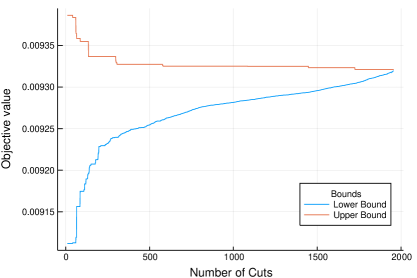
Figure 1: Convergence of Algorithm 3 on the OR-library problem port2 with a minimum return constraint and a cardinality constraint $\|\bm{x}\|_{0}\leq 5$. The behavior shown here is typical.

5 Computational Experiments on Real-World Data

In this section, we evaluate our outer-approximation method, implemented in Julia $1.1$ using the JuMP.jl package version $0.18.5$ and solved using CPLEX version $12.8.0$ for the master problems, and Mosek version $9.0$ for the continuous quadratic subproblems. We compare the method against big-$M$ and MISOCO formulations of Problem (4), solved in CPLEX. To bridge the gap between theory and practice, we have made our code freely available on Github at github.com/ryancorywright/SparsePortfolioSelection.jl.

All experiments were performed on a MacBook Pro with a $2.9$GHz i$9$ Intel®CPU and $16$GB DDR$4$ Memory. For simplicity, we ran all methods on one thread, using default CPLEX parameters.

In all experiments which do not involve minimum investment constraints, we solve the following optimization problem, which places a multiplier $\kappa$ on the return term but—since the multiplier can be absorbed into the return vector $\bm{\mu}$—is mathematically equivalent to Problem (4):

$$\min_{\bm{x}\in\mathbb{R}^{n}_{+}}\ \frac{1}{2}\bm{x}^{\top}\bm{\Sigma}\bm{x}+\frac{1}{2\gamma}\|\bm{x}\|_{2}^{2}-\kappa\bm{\mu}^{\top}\bm{x}\quad\text{s.t.}\quad\bm{l}\leq\bm{A}\bm{x}\leq\bm{u},\ \bm{e}^{\top}\bm{x}=1,\ \|\bm{x}\|_{0}\leq k.$$ (34)

Note that we only consider cases where $\kappa=0$ or $\kappa=1$, depending on whether we are penalizing low expected return portfolios in the objective or constraining the portfolios expected return.

In the presence of minimum investment constraints, we augment Problem (34) with the constraints $x_{i}\geq z_{i}x_{i,\min}$, which can be straightforwardly managed by the algorithms derived in this paper in the manner discussed in Section 5.2.

We aim to answer the following questions:

1. How does Algorithm 3 compare to existing commercial codes such as CPLEX?

2. How do constraints affect Algorithm 3’s scalability?

3. How does Algorithm 3 scale as a function of the number of securities in the buyable universe?

4. How sensitive are optimal solutions to Problem (4) to the hyperparameters $\kappa,\gamma,k$?

5.1 A Comparison Between Algorithm 3 and Existing Commercial Codes

We now present a direct comparison of Algorithm 3 with CPLEX version $12.8.0$, where CPLEX uses both big-M and MISOCO formulations of Problem (4). Note that the MISOCO formulation which we pass directly to CPLEX is (cf. Ben-Tal and Nemirovski 2001, Aktürk et al. 2009):

$$\min_{\bm{z}\in\mathcal{Z}_{k}^{n},\bm{x}\in\mathbb{R}_{+}^{n},\bm{\theta}\in\mathbb{R}_{+}^{n}}\ \frac{1}{2}\bm{x}^{\top}\bm{\Sigma}\bm{x}+\frac{1}{2\gamma}\bm{e}^{\top}\bm{\theta}-{\color[rgb]{0,0,0}\kappa}\bm{\mu}^{\top}\bm{x}\quad\text{s.t.}\quad\bm{l}\leq\bm{A}\bm{x}\leq\bm{u},\ \bm{e}^{\top}\bm{x}=1,\ x_{i}^{2}\leq z_{i}\theta_{i}\quad\forall i\in[n].$$ (35)

We remark that CPLEX’s MISOCO routine can be interpreted as an aggregation of the techniques reviewed in the introduction, since CPLEX mines the optimization literature for techniques which improve its performance. For instance, as discussed by Vielma (2017), CPLEX’s MISOCO routine currently includes the conic disaggregation technique of Vielma et al. (2017). Indeed, this aggregation has been so successful that Bienstock (2010) showed that, in $2010$, CPLEX outperformed several of the methods reviewed in the introduction.

We compare the three approaches in two distinct situations. First, when no constraints are applied and the system $\bm{l}\leq\bm{A}\bm{x}\leq\bm{u}$ is empty, and second when a minimum return constraint is applied, i.e., $\bm{\mu}^{\top}\bm{x}\geq\bar{r}$. In the former case we set $\kappa=1$, while in the latter case we set $\kappa=0$ and as suggested by Cesarone et al. (2009), Zheng et al. (2014) we set $\bar{r}$ in the following manner: Let

$$r_{\min}= \bm{\mu}^{\top}\bm{x}_{\min} \ \bm{x}_{\min}=\arg\min_{\bm{x}}\quad\frac{1}{2}\bm{x}^{\top}\left(\frac{1}{\gamma}\mathbb{I}+\bm{\Sigma}\right)\bm{x}\quad \text{s.t.}\quad\bm{e}^{\top}\bm{x}=1,\bm{x}\geq\bm{0},$$ where

$$r_{\max}= \bm{\mu}^{\top}\bm{x}_{\max} \ \bm{x}_{\max}=\arg\max_{\bm{x}}\quad\bm{\mu}^{\top}\bm{x}-\frac{1}{2\gamma}\bm{x}^{\top}\bm{x}\quad \text{s.t.}\quad\bm{e}^{\top}\bm{x}=1,\bm{x}\geq\bm{0},$$ where

and set $\bar{r}=r_{\min}+0.3(r_{\max}-r_{\min})$.

Table 3 (resp. Table 4) depicts the time required for all $3$ approaches to determine an optimal allocation of funds without (resp. with) the minimum return constraint. The problem data is taken from the $5$ mean-variance portfolio optimization problems described by Chang et al. (2000) and included in the OR-library test set by Beasley (1990). Note that we turned off the second-order cone lower bound for these tests, and ensured feasibility in the master problem by imposing $\sum_{i\in[n]:\mu_{i}\geq\bar{r}}z_{i}\geq 1$ when running Algorithm 3 on the instances with a minimum return constraint (see Section 3.2). Furthermore, as Algorithm 3 is slow to converge for some instances with a return constraint, in Table 4 we ran the method after applying $50$ cuts at the root node, generated using the in-out method (see Appendix 8, for the relevant pseudocode).

Table 3: Runtime in seconds per approach with $\kappa=1$, $\gamma=\frac{100}{\sqrt{n}}$ and no constraints in the system $\bm{l}\leq\bm{A}\bm{x}\leq\bm{u}$. We impose a time limit of $300$s and run all approaches on one thread. If a solver fails to converge, we report the number of explored nodes at the time limit.

Problem	$n$	$k$	Algorithm 3			CPLEX Big-M		CPLEX MISOCO
			Time	Nodes	Cuts	Time	Nodes	Time	Nodes
port $1$	$31$	$5$	$0.17$	$0$	$4$	$1.98$	$31,640$	0.03	$0$
		$10$	$0.16$	$0$	$4$	$1.11$	$16,890$	0.01	$0$
		$20$	$0.14$	$0$	$4$	0.01	$108$	$0.03$	$0$
port $2$	$85$	$5$	0.01	$0$	$4$	$>300$	$1,968,000$	$0.11$	$0$
		$10$	0.01	$0$	$4$	$>300$	$2,818,000$	$0.12$	$0$
		$20$	0.01	$0$	$4$	$>300$	$3,152,000$	$0.29$	$0$
port $3$	$89$	$5$	0.01	$0$	$8$	$>300$	$2,113,000$	$0.38$	$0$
		$10$	0.01	$0$	$4$	$>300$	$2,873,000$	$0.41$	$0$
		$20$	0.02	$0$	$4$	$>300$	$2,998,000$	$0.11$	$0$
port $4$	$98$	$5$	0.03	$0$	$8$	$>300$	$1,888,000$	$0.41$	$0$
		$10$	0.02	$0$	$8$	$>300$	$2,457,000$	$2.74$	$3$
		$20$	0.03	$0$	$9$	$>300$	$2,454,000$	$0.38$	$0$
port $5$	$225$	$5$	0.15	$0$	$9$	$>300$	$676,300$	$11.17$	$9$
		$10$	0.02	$0$	$4$	$>300$	$926,600$	$3.04$	$0$
		$20$	0.03	$0$	$7$	$>300$	$902,100$	$2.88$	$0$

Table 4: Runtime in seconds per approach with $\kappa=0$, $\gamma=\frac{100}{\sqrt{n}}$ and a minimum return constraint $\bm{\mu}^{\top}\bm{x}\geq\bar{r}$. We impose a time limit of $3600$s and run all approaches on one thread. If a solver fails to converge, we report the number of explored nodes at the time limit.

Problem	$n$	$k$	Algorithm 3			Algorithm 3+in-out			CPLEX Big-M		CPLEX MISOCO
			Time	Nodes	Cuts	Time	Nodes	Cuts	Time	Nodes	Time	Nodes
port $1$	$31$	$5$	0.22	$161$	$32$	$0.23$	$113$	$19$	$9.32$	$119,200$	$0.83$	$47$
		$10$	0.20	$159$	$28$	$0.25$	$86$	$25$	$1970$	$30,430,000$	$0.84$	$44$
		$20$	$0.16$	$0$	$7$	$0.16$	$0$	$4$	$258.4$	$4,966,000$	0.05	$0$
port $2$	$85$	$5$	$48.29$	$73,850$	$1,961$	31.47	$42,950$	$1,272$	$>3,600$	$15,020,000$	$91.98$	$1,163$
		$10$	$807.3$	$243,500$	$6,433$	$891.97$	$255,200$	$6,019$	$>3,600$	$20,890,000$	82.44	$902$
		$20$	10.52	$12,260$	$1,224$	$13.0$	$13,650$	$1,350$	$>3,600$	$21,060,000$	$24.54$	$210$
port $3$	$89$	$5$	$175.2$	$132,700$	$3,187$	151.1	$96,010$	$2,345$	$>3,600$	$14,680,000$	$213.3$	$2,528$
		$10$	$>3,600$	$439,400$	$9,851$	$>3,600$	$490,400$	$11,310$	$>3,600$	$20,710,000$	531.3	$5,776$
		$20$	$119.5$	$65,180$	$4,473$	$60.03$	$40,240$	$3,275$	$>3,600$	$22,240,000$	21.32	$170$
port $4$	$98$	$5$	$2,690$	$479,700$	$11,320$	2,475	$499,700$	$11,040$	$>3,600$	$12,426,000$	$2779$	$25,180$
		$10$	$>3,600$	$311,200$	$12,400$	$>3,600$	$320,700$	$14,790$	$>3,600$	$20,950,000$	$>3,600$	$30,190$
		$20$	$1,638$	$241,600$	$10,710$	$2,067$	$279,500$	$12,760$	$>3,600$	$21,470,000$	148.9	$1,115$
port $5$	$225$	$5$	$0.85$	$1,489$	$202$	0.40	$560$	$74$	$>3,600$	$5,000,000$	$28.3$	$22$
		$10$	$0.60$	$73$	$41$	0.03	$2$	$5$	$>3,600$	$8,989,000$	$3.33$	$0$
		$20$	$0.39$	$63$	$52$	0.08	$0$	$11$	$>3,600$	$10,960,000$	$115.02$	$90$

Table 4 indicates that the port$4$ instance cannot be solved to certifiable optimality by any approach within an hour when $k=10$, in the presence of a minimum return constraint. Nonetheless, both Algorithm 3 and CPLEX’s MISOCO method obtain solutions which are certifiably within $1\%$ of optimality very quickly. Indeed, Table 5 depicts the bound gaps of all $3$ approaches at $120$s on these problems; Algorithm 3 never has a bound gap larger than $0.5\%$.

Table 5: Bound gap at $120$s per approach with $\kappa=0$, $\gamma=\frac{100}{\sqrt{n}}$ and a minimum return constraint $\bm{\mu}^{\top}\bm{x}\geq\bar{r}$. We run all approaches on one thread.

Problem	$n$	$k$	Algorithm 3			Algorithm 3+in-out			CPLEX Big-M		CPLEX MISOCO
			Gap ($\%$)	Nodes	Cuts	Gap ($\%$)	Nodes	Cuts	Gap ($\%$)	Nodes	Gap ($\%$)	Nodes
port $2$	$85$	$5$	0	$73,850$	$1,961$	0	$42,950$	$1,272$	$84.36$	$611,500$	0	$1,163$
		$10$	$0.26$	$90,670$	$3,463$	$0.15$	$72,240$	$3,366$	$425.2$	$1,057,000$	0	$902$
		$20$	0	$12,260$	$1,224$	0	$13,650$	$1,350$	$65.96$	$1,367,000$	0	$210$
port $3$	$89$	$5$	$0.1$	$123,100$	$2,308$	0.08	$78,950$	$2,137$	$88.48$	$634,300$	$0.27$	$1,247$
		$10$	$0.29$	$65,180$	$4,473$	$0.21$	$62,840$	$3,503$	$452.4$	$1,073,000$	0.19	$1,246$
		$20$	0	$60,090$	$3,237$	0	$40,240$	$3,275$	$67.55$	$1,280,000$	0	$170$
port $4$	$98$	$5$	0.18	$55,460$	$3,419$	$0.37$	$53,780$	$3,648$	$87.67$	$541,800$	$0.60$	$888$
		$10$	$0.46$	$51,500$	$3,704$	0.29	$46,700$	$3,241$	$84.22$	$1,018,000$	0.29	$977$
		$20$	$0.17$	$57,990$	$3,393$	$0.13$	$59,820$	$3,886$	$71.42$	$1,163,000$	0.05	$846$

The experimental results illustrate that our approach is several orders of magnitude more efficient than the big-$M$ approach on all problems considered, and performs comparably with the MISOCO approach. Moreover, our approach’s edge over CPLEX increases with the problem size.

Our main findings from this set of experiments are as follows:

1. For problems with unit simplex constraints, big-$M$ approaches do not scale to real-world problem sizes in the presence of ridge regularization, because they cannot exploit the ridge regularizer and therefore obtain low-quality lower bounds, even after expanding a large number of nodes. This poor performance is due to the ridge regularizer; the big-$M$ approach typically exhibits better performance than this in numerical studies done without a regularizer.

2. MISOCO approaches perform competitively, and are often a computationally reasonable approach for small to medium sized instances of Problem (4), as they are easy to implement and typically have bound gaps of $<1\%$ in instances where they fail to converge within the time budget.

3. Varying the cardinality of the optimal portfolio does not affect solve times substantially without a minimum return constraint, although it has a nonlinear effect with this constraint.

For the rest of the paper, we do not consider big-$M$ formulations of Problem (4), as they do not scale to larger problems with $200$ or more securities in the universe of buyable assets.

5.2 Benchmarking Algorithm 3 in the Presence of Minimum Investment Constraints

In this section, we explore Algorithm 3’s scalability in the presence of minimum investment constraints, by solving the problems generated by Frangioni and Gentile (2006) and subsequently solved by Frangioni and Gentile (2007), Frangioni and Gentile (2009), Zheng et al. (2014) among others. These problems have minimum investment, maximum investment, and minimum return constraints, which render many entries in $\mathcal{Z}^{n}_{k}$ infeasible. Therefore, to avoid generating an excessive number of feasibility cuts, we use the copy of variables technique suggested in Section 3.2.

Additionally, as the covariance matrices in these problems are highly diagonally dominant (with much larger on-diagonal entries than off-diagonal entries), the method does not converge quickly if we do not extract any diagonal dominance. Indeed, Appendix 7.1 shows that the method often fails to converge within $600$s for the problems studied in this section when we do not extract a diagonally dominant term. Therefore, we first preprocess the covariance matrices to extract more diagonal dominance, as discussed in Section 3.2. Note that we need not actually solve any SDOs to preprocess the data, as high quality diagonal matrices for this problem data have been made publicly available by Frangioni et al. (2017) at http://www.di.unipi.it/optimize/Data/MV/diagonals.tgz (specifically, we use the entries in the “s” folder of this repository). After reading in their diagonal matrix $\bm{D}$, we replace $\bm{\Sigma}$ with $\bm{\Sigma}-\bm{D}$ and use the regularizer $\gamma_{i}$ for each index $i$, where $\gamma_{i}=\left(\frac{1}{\gamma}+D_{i,i}\right)^{-1}$ (we do this for all approaches benchmarked here, including CPLEX’s MISOCO routine).

We now compare the times for Algorithm 3 and CPLEX’s MISOCO routines to solve the diagonally dominant instances in the dataset generated by Frangioni and Gentile (2006), along with a variant of Algorithm 3 where we use the in-out method at the root node, and another variant where we apply the in-out method at both the root node and $50$ additional nodes. In all cases, we take $\gamma=\frac{1000}{n}$, which ensures that $\gamma_{i}\approx\frac{1}{D_{i,i}}$, since on this dataset $\frac{1}{2\gamma}$ is around $5$ orders of magnitude smaller than $D_{i,i}$ and thus the net contribution of the regularization term to the objective is negligible. Table 6 depicts the average time taken by each approach, and demonstrates that Algorithm 3 substantially outperforms CPLEX, particularly for problems without an explicit cardinality constraint, but with an implicit cardinality constraint of $\|\bm{x}\|_{0}\leq k$ for $k\leq 13$ due to the minimum investment constraints $x_{i}\geq l_{i}z_{i}$ where $l_{i}$ is uniformly drawn from $[0.075,0.125]$ (Frangioni and Gentile 2007). We provide the full instance-wise results in Appendix 7.1, and also consider the possibility of supplying the cuts from the in-out method to CPLEX before running the MISOCP method therein.

Table 6: Average runtime in seconds per approach with $\kappa=0$, $\gamma=\frac{1000}{n}$ for the problems generated by Frangioni and Gentile (2006). We impose a time limit of $600$s and run all approaches on one thread. If a solver fails to converge, we report the number of explored nodes at the time limit, use $600$s in lieu of the solve time, and report the number of failed instances (out of $10$) next to the solve time in brackets. Note that the minimum investment constraints impose an implicit cardinality constraint with $k\approx{\color[rgb]{0,0,0}13}$.

Problem	$k$	Algorithm 3			Algorithm 3 $+$ in-out			Algorithm 3 in-out $+$ 50			CPLEX MISOCO
		Time	Nodes	Cuts	Time	Nodes	Cuts	Time	Nodes	Cuts	Time	Nodes
200+	6	1.55	1,298	236.3	1.77	1,262	209.4	7.4	910.4	118	87.74 (0)	95.3
200+	8	1.95	1,968	260.3	2.30	1,626	217	7.97	949.1	97.3	73.42 (0)	79.8
200+	10	7.74	7,606	509.7	4.33	3,686	298.9	10.35	2,066	175.5	161.9 (0)	184
200+	12	25.57	28,830	203.8	2.06	1,764	71.6	9.04	1,000	33.9	353.1 (4)	398.1
200+	200	18.71	23,190	208.4	2.79	2,288	92	10	1,394	56.1	599.3 (9)	735.1
300+	6	16.83	9,141	974.2	23.59	8,025	864.1	29.92	5,738	565.9	434.5 (3)	157.6
300+	8	44.68	21,050	1,577	64.46	19,682	1457.8	61.0	14,236	1,036	489.5 (5)	174.0
300+	10	88.57	44,160	1,901	78.05	33,253	1438.4	110.2	24,487	971.5	472.0 (5)	171.9
300+	12	16.16	13,880	262.7	4.65	3,181	127.4	15.94	1475	66.7	401.5 (4)	158.2
300+	300	21.36	18,140	262.1	9.24	6,288	191.9	24.33	5,971	168.4	600.0 (10)	219.2
400+	6	54.47	13,330	1,717	66.52	12,160	1,619	85.51	11,070	1,402	531.7 (8)	84.0
400+	8	173.8	35,390	2,828	160.9	32,930	2,709	163.3	28,020	2,363	534.0 (8)	80.8
400+	10	158.0	55,490	1,669	104.5	32,314	1369.7	81.48	22,130	824.9	517.9 (8)	74.8
400+	12	3.97	4,324	116.6	1.9	1,214	48.6	15.67	627.4	29.8	478.0 (4)	75.3
400+	400	8.68	7,540	120.5	5.19	3,539	88.8	21.31	3,210	79.4	600.0 (10)	74.2

Our main findings from this experiment are as follows:

• Algorithm 3 outperforms CPLEX in the presence of minimum investment constraints. Interestingly, the log output indicates that CPLEX’s custom heuristics typically obtain incumbent solutions which are better than those obtained by Algorithm 2 and supplied to Algorithm 3 as a warm-start. This suggests that Algorithm 3’s superior numerical performance arises because it can develop high-quality (i.e., better than the SOCO bound) lower bounds more quickly. This shouldn’t be too surprising, since beating a continuous relaxation bound involves branching (or cutting), which is cheaper to perform on a pure binary formulation than a MISOCO formulation.

• Running the in-out method at the root node improves solve times when $k\geq 10$, but does more harm than good when $k<10$, because in the latter case Algorithm 3 already performs well.

• Running the in-out method at non-root nodes does more harm than good for easy problems, but improves solve times for larger problems ($400+$ with $k\in\{8,10\}$), as reported in Appendix 7.1.

• With a cardinality constraint, Algorithm 3’s solve times are comparable to those reported by Zheng et al. (2014), Frangioni et al. (2016) (note however that this comparison is imperfect since all three approaches were run on different machines; the source code for the other two approaches is unavailable and hence we cannot obtain truly comparable data). This can be explained by the fact that all three methods solve these problems in $10$s of seconds, and thus these problems can be viewed as “easy”. Without an explicit cardinality constraint (but with minimum investment constraints which impose an implicit cardinality constraint of $k\approx 13$ Frangioni and Gentile (2007)), our solve times are two orders of magnitude faster than those reported by Zheng et al. (2014)’s (an average of $580$s for $400+$), and an order of magnitude faster than those by Frangioni et al. (2016) (an average of $52$s for $400+$).

• As shown in Appendix 7.1, applying the diagonal dominance preprocessing technique proposed by Frangioni and Gentile (2007) yields faster solve times than applying the technique proposed by Zheng et al. (2014), even though the latter technique yields tighter continuous relaxations (Zheng et al. 2014). This might occur because Frangioni and Gentile (2007)’s technique prompts our approach to make better branching decisions and/or Zheng et al. (2014)’s approach is only guaranteed to yield tighter continuous relaxations before (i.e., not after) branching.

• As shown in Appendix 7.1, passing the cuts generated by the in-out method to CPLEX does more harm than good. This can be explained by the fact that the SOCP relaxation, which is very affordable to compute, is at least as strong as the lower approximation generated by the in-out method (indeed, the in-out method can be interpreted as a linearization of the SOCP relaxation about a “cleverly” sampled set of points), while providing the in-out method’s lower approximation to CPLEX increases the amount of work which CPLEX needs to perform at each node in the branch-and-bound tree.

5.3 Exploring the Scalability of Algorithm 3

In this section, we explore Algorithm 3’s scalability with respect to the number of securities in the buyable universe, by measuring the time required to solve several large-scale sparse portfolio selection problems to provable optimality: the S$\&$P $500$, the Russell $1000$, and the Wilshire $5000$. In all three cases, the problem data is taken from daily closing prices from January $3$ $2007$ to December $29$ $2017$, which are obtained from Yahoo! Finance via the R package quantmod (see Ryan and Ulrich (2018)), and rescaled to correspond to a holding period of one month. We apply Singular Value Decomposition to obtain low-rank estimates of the correlation matrix, and rescale the low-rank correlation matrix by each asset’s variance to obtain a low-rank covariance matrix $\bm{\Sigma}$. We also omit days with a greater than $20\%$ change in closing prices when computing the mean and covariance for the Russell $1000$ and Wilshire $5000$, since these changes occur on low-volume trading and typically reverse the next day.

Tables 7–9 depict the times required for Algorithm 3 and CPLEX MISOCO to solve the problem to provable optimality for different choices of $\gamma$, $k$, and Rank$(\bm{\Sigma})$. In particular, they depict the time taken to solve (a) an unconstrained problem where $\kappa=1$ and (b) a constrained problem where $\kappa=0$ containing a minimum return constraint computed in the same fashion as in Section 5.1.

Table 7: Runtimes in seconds per approach for the S$\&$P $500$ with $\kappa=1$ (left); $\kappa=0$ and a minimum return constraint (right), a one-month holding period and a runtime limit of $600$s. For instances with a minimum return constraint where $\gamma=\frac{100}{\sqrt{n}}$, we run the in-out method at the root node before running Algorithm 3. We run all approaches on one thread. When a method fails to converge, we report the bound gap at $600$s.

$\gamma$	Rank$(\bm{\Sigma})$	$k$	Algorithm 3			CPLEX MISOCO		Algorithm 3			CPLEX MISOCO
			Time	Nodes	Cuts	Time	Nodes	Time	Nodes	Cuts	Time	Nodes
$\frac{1}{\sqrt{n}}$	$50$	$10$	$0.01$	$0$	$4$	$0.54$	$0$	$0.01$	$0$	$3$	$73.28$	$210$
		$50$	$0.02$	$0$	$4$	$0.49$	$0$	$0.28$	$108$	$45$	$78.59$	$499$
		$100$	$0.03$	$0$	$4$	$1.00$	$0$	$0.05$	$7$	$7$	$0.97$	$0$
		$200$	$0.06$	$0$	$4$	$0.86$	$0$	$0.08$	$1$	$5$	$53.53$	$300$
$\frac{1}{\sqrt{n}}$	$100$	$10$	$0.01$	$0$	$4$	$1.49$	$0$	$2.01$	$972$	$344$	$339.8$	$420$
		$50$	$0.02$	$0$	$4$	$1.36$	$0$	$0.32$	$104$	$41$	$283.8$	$410$
		$100$	$0.04$	$0$	$4$	$1.30$	$0$	$0.06$	$5$	$7$	$286.2$	$520$
		$200$	$0.09$	$0$	$4$	$3.10$	$0$	$0.06$	$0$	$3$	$472.7$	$990$
$\frac{1}{\sqrt{n}}$	$150$	$10$	$0.01$	$0$	$4$	$2.61$	$0$	$3.96$	$1,633$	$410$	$268.3$	$157$
		$50$	$0.03$	$0$	$4$	$2.23$	$0$	$0.29$	$62$	$33$	$265.6$	$200$
		$100$	$0.06$	$0$	$4$	$4.71$	$0$	$0.07$	$0$	$6$	$394.9$	$340$
		$200$	$0.14$	$0$	$4$	$4.80$	$0$	$0.13$	$0$	$3$	$6.20$	$0$
$\frac{1}{\sqrt{n}}$	$200$	$10$	$0.01$	$0$	$4$	$2.74$	$0$	$5.20$	$2,804$	$450$	$345.0$	$171$
		$50$	$0.03$	$0$	$4$	$3.14$	$0$	$0.49$	$86$	$47$	$337.7$	$210$
		$100$	$0.06$	$0$	$4$	$17.27$	$3$	$0.15$	$5$	$8$	$104.2$	$40$
		$200$	$0.13$	$0$	$4$	$105.2$	$60$	$0.10$	$0$	$3$	$46.18$	$10$
$\frac{100}{\sqrt{n}}$	$50$	$10$	$0.01$	$0$	$4$	$0.51$	$0$	$0.09\%$	$70,200$	$3,855$	$0.10\%$	$1,600$
		$50$	$0.02$	$0$	$4$	$1.14$	$0$	$0.77$	$309$	$113$	$268.5$	$841$
		$100$	$0.03$	$0$	$4$	$0.68$	$0$	$0.09$	$0$	$8$	$1.66$	$0$
		$200$	$0.07$	$0$	$4$	$1.04$	$0$	$0.16$	$0$	$4$	$15.26$	$10$
$\frac{100}{\sqrt{n}}$	$100$	$10$	$0.01$	$0$	$4$	$1.30$	$0$	$0.26\%$	$54,000$	$4,721$	$0.24\%$	$598$
		$50$	$0.03$	$0$	$4$	$3.48$	$0$	$0.07$	$1$	$7$	$0.28\%$	$291$
		$100$	$0.06$	$0$	$5$	$5.93$	$0$	$0.11$	$0$	$4$	$0.29\%$	$352$
		$200$	$0.13$	$0$	$5$	$2.16$	$0$	$0.14$	$0$	$5$	$301.3$	$380$
$\frac{100}{\sqrt{n}}$	$150$	$10$	$0.02$	$0$	$4$	$2.00$	$0$	$0.33\%$	$46,720$	$4,437$	$0.28\%$	$345$
		$50$	$0.04$	$0$	$4$	$34.57$	$20$	$0.09$	$0$	$6$	$0.28\%$	$291$
		$100$	$0.06$	$0$	$4$	$27.76$	$20$	$0.11$	$0$	$4$	$0.29\%$	$352$
		$200$	$0.10$	$0$	$4$	$26.93$	$20$	$0.35$	$0$	$6$	$344.3$	$270$
$\frac{100}{\sqrt{n}}$	$200$	$10$	$0.02$	$0$	$4$	$7.77$	$0$	$0.45\%$	$56,100$	$4,336$	$0.36\%$	$280$
		$50$	$0.04$	$0$	$4$	$48.75$	$20$	$0.20$	$1$	$19$	$0.35\%$	$256$
		$100$	$0.10$	$0$	$5$	$44.02$	$20$	$0.15$	$0$	$5$	$104.2$	$40$
		$200$	$0.16$	$0$	$4$	$36.57$	$20$	$0.18$	$0$	$4$	$76.80$	$10$

Table 8: Runtimes in seconds per approach for the Russell $1000$ with $\kappa=1$ (left); $\kappa=0$ and a minimum return constraint (right), a one-month holding period and a runtime limit of $600$s. For instances with a minimum return constraint, we run the in-out method at the root node before running Algorithm 3. We run all approaches on one thread. When a method fails to converge, we report the bound gap at $600$s.

$\gamma$	Rank$(\bm{\Sigma})$	$k$	Algorithm 3			CPLEX MISOCO		Algorithm 3			CPLEX MISOCO
			Time	Nodes	Cuts	Time	Nodes	Time	Nodes	Cuts	Time	Nodes
$\frac{1}{\sqrt{n}}$	$50$	$10$	$0.02$	$0$	$6$	$7.77$	$3$	$12.38$	$2467$	$316$	$0.01\%$	$545$
		$50$	$0.06$	$0$	$12$	$9.19$	$7$	$0.32$	$0$	$7$	$0.01\%$	$900$
		$100$	$0.04$	$0$	$5$	$0.92$	$0$	$0.81$	$10$	$14$	$0.01\%$	$1,048$
		$200$	$0.07$	$0$	$5$	$1.83$	$0$	$0.46$	$1$	$14$	$0.01\%$	$1,043$
$\frac{1}{\sqrt{n}}$	$100$	$10$	$0.03$	$3$	$7$	$13.27$	$5$	$272.3$	$49,200$	$1,266$	$0.01\%$	$400$
		$50$	$0.09$	$2$	$12$	$154.0$	$90$	$1.32$	$10$	$13$	$0.01\%$	$400$
		$100$	$0.05$	$0$	$5$	$2.83$	$0$	$15.52$	$5,271$	$250$	$0.01\%$	$599$
		$200$	$0.14$	$0$	$8$	$335.9$	$260$	$2.12$	$111$	$64$	$0.01\%$	$399$
$\frac{1}{\sqrt{n}}$	$200$	$10$	$0.05$	$2$	$10$	$41.08$	$7$	$24.14$	$8,200$	$318$	$31.20\%$	$138$
		$50$	$0.16$	$8$	$14$	$344.0$	$60$	$0.01\%$	$86,020$	$1,433$	$0.02\%$	$100$
		$100$	$0.08$	$0$	$5$	$60.54$	$10$	$4.88$	$131$	$41$	$0.01\%$	$100$
		$200$	$0.16$	$0$	$5$	$6.79$	$0$	$0.01\%$	$64,600$	$1,049$	$4.00\%$	$100$
$\frac{1}{\sqrt{n}}$	$300$	$10$	$0.06$	$1$	$10$	$175.9$	$15$	$9.00$	$1,200$	$246$	$0.01\%$	$70$
		$50$	$0.16$	$2$	$13$	$323.3$	$31$	$0.02\%$	$61,100$	$1,227$	$63.35\%$	$78$
		$100$	$0.16$	$0$	$8$	$260.4$	$30$	$0.02\%$	$48,550$	$856$	$3.01\%$	$64$
		$200$	$0.31$	$0$	$8$	$0.01\%$	$464$	$0.01\%$	$29,480$	$786$	$6.00\%$	$75$
$\frac{100}{\sqrt{n}}$	$50$	$10$	$0.04$	$1$	$11$	$7.58$	$3$	$0.59\%$	$62,050$	$2,553$	$0.39\%$	$700$
		$50$	$0.04$	$0$	$9$	$2.34$	$0$	$0.61\%$	$114,000$	$1,531$	$0.32\%$	$837$
		$100$	$0.36$	$0$	$4$	$2.57$	$0$	$112.1$	$42,661$	$787$	$0.12\%$	$993$
		$200$	$0.09$	$0$	$5$	$1.25$	$0$	$0.40$	$0$	$19$	$135.4$	$220$
$\frac{100}{\sqrt{n}}$	$100$	$10$	$0.03$	$2$	$9$	$11.50$	$5$	$0.77\%$	$69,800$	$2,599$	$0.55\%$	$400$
		$50$	$0.06$	$0$	$8$	$65.82$	$40$	$0.68\%$	$93,580$	$1,472$	$0.38\%$	$400$
		$100$	$0.06$	$0$	$5$	$22.82$	$10$	$0.43\%$	$82,500$	$1,359$	$0.46\%$	$470$
		$200$	$0.11$	$0$	$5$	$42.68$	$30$	$0.34$	$0$	$13$	$0.37\%$	$400$
$\frac{100}{\sqrt{n}}$	$200$	$10$	$0.06$	$1$	$10$	$31.33$	$0$	$0.84\%$	$84,617$	$2,183$	$1.23\%$	$126$
		$50$	$0.10$	$1$	$10$	$164.4$	$30$	$1.55\%$	$99,600$	$1,576$	$1.31\%$	$100$
		$100$	$0.08$	$0$	$4$	$71.91$	$10$	$0.92\%$	$69,850$	$1,279$	$9.36\%$	$118$
		$200$	$0.16$	$0$	$5$	$50.98$	$10$	$0.35$	$1$	$10$	$2.20\%$	$123$
$\frac{100}{\sqrt{n}}$	$300$	$10$	$0.06$	$1$	$12$	$134.1$	$15$	$0.94\%$	$72,400$	$2,759$	$1.00\%$	$65$
		$50$	$0.10$	$0$	$8$	$207.7$	$20$	$1.78\%$	$58,740$	$1,363$	$48.31\%$	$62$
		$100$	$0.10$	$0$	$4$	$544.3$	$50$	$1.16\%$	$55,810$	$1,027$	$14.40\%$	$61$
		$200$	$0.20$	$0$	$5$	$221.4$	$30$	$1.04\%$	$61,410$	$1,122$	$2.92\%$	$61$

Table 9: Runtimes in seconds per approach for the Wilshire $5000$ with $\kappa=1$ (left); $\kappa=0$ and a minimum return constraint (right), a one-month holding period and a runtime limit of $600$s. For instances with a minimum return constraint where $\gamma=\frac{100}{\sqrt{n}}$, we run the in-out method at the root node before running Algorithm 3. We run all approaches on one thread. When a method fails to converge, we report the bound gap at $600$s (using the symbol “$-$” to denote that a method failed to produce a feasible solution).

$\gamma$	Rank$(\bm{\Sigma})$	$k$	Algorithm 3			CPLEX MISOCO		Algorithm 3			CPLEX MISOCO
			Time	Nodes	Cuts	Time	Nodes	Time	Nodes	Cuts	Time	Nodes
$\frac{1}{\sqrt{n}}$	$100$	$10$	$0.04$	$0$	$4$	$15.07$	$0$	$1.95$	$0$	$2$	$50.0\%$	$122$
		$50$	$0.07$	$0$	$10$	$244.8$	$29$	$2.32$	$0$	$2$	$32.0\%$	$132$
		$100$	$0.22$	$0$	$4$	$30.08$	$2$	$0.59$	$10$	$9$	$62.0\%$	$127$
		$200$	$0.24$	$0$	$4$	$40.54$	$3$	$0.27$	$0$	$6$	$44.5\%$	$100$
$\frac{1}{\sqrt{n}}$	$200$	$10$	$0.07$	$0$	$6$	$70.12$	$2$	$2.34$	$0$	$8$	$30.0\%$	$43$
		$50$	$0.08$	$0$	$8$	$392.5$	$25$	$5.54$	$31$	$17$	$74.0\%$	$40$
		$100$	$0.08$	$0$	$5$	$0.01\%$	$91$	$1.70$	$0$	$12$	$62.0\%$	$44$
		$200$	$0.25$	$0$	$4$	$49.26$	$0$	$0.01\%$	$8,451$	$361$	$41.5\%$	$40$
$\frac{1}{\sqrt{n}}$	$500$	$10$	$0.15$	$10$	$11$	$0.01\%$	$13$	$10.53$	$300$	$66$	$-$	$5$
		$50$	$0.54$	$0$	$8$	$0.01\%$	$30$	$0.01\%$	$49,000$	$805$	$-$	$6$
		$100$	$0.20$	$0$	$6$	$492.7$	$3$	$0.01\%$	$36,670$	$1,068$	$-$	$5$
		$200$	$0.57$	$0$	$5$	$0.01\%$	$20$	$3.41$	$0$	$14$	$-$	$5$
$\frac{1}{\sqrt{n}}$	$1,000$	$10$	$0.48$	$35$	$28$	$0.01\%$	$9$	$0.01\%$	$40,500$	$1,130$	$-$	$2$
		$50$	$1.08$	$20$	$29$	$0.01\%$	$9$	$0.02\%$	$56,800$	$937$	$-$	$2$
		$100$	$0.44$	$0$	$7$	$0.01\%$	$11$	$0.02\%$	$25,040$	$523$	$-$	$2$
		$200$	$0.56$	$0$	$4$	$0.01\%$	$10$	$2.61$	$1$	$12$	$-$	$2$
$\frac{100}{\sqrt{n}}$	$100$	$10$	$0.03$	$0$	$5$	$29.30$	$2$	$0.28\%$	$24,870$	$1,178$	$50.1\%$	$91$
		$50$	$0.04$	$0$	$5$	$39.08$	$3$	$0.38\%$	$45,810$	$636$	$62.1\%$	$82$
		$100$	$0.07$	$0$	$5$	$200.0$	$11$	$0.12\%$	$55,700$	$912$	$45.1\%$	$80$
		$200$	$0.10$	$0$	$10$	$99.07$	$10$	$0.49$	$0$	$10$	$22.1\%$	$91$
$\frac{100}{\sqrt{n}}$	$200$	$10$	$0.06$	$0$	$8$	$56.48$	$2$	$0.38\%$	$34,100$	$1,071$	$-$	$29$
		$50$	$0.08$	$0$	$7$	$78.00$	$3$	$0.47\%$	$40,340$	$1,034$	$66.1\%$	$30$
		$100$	$0.20$	$0$	$5$	$0.01\%$	$20$	$0.43\%$	$15,010$	$325$	$45.1\%$	$33$
		$200$	$0.14$	$0$	$4$	$224.4$	$10$	$0.98$	$6$	$10$	$20.1\%$	$30$
$\frac{100}{\sqrt{n}}$	$500$	$10$	$0.15$	$5$	$13$	$0.01\%$	$16$	$0.52\%$	$32,920$	$1,235$	$-$	$4$
		$50$	$0.08$	$0$	$4$	$0.01\%$	$6$	$1.11\%$	$65,560$	$771$	$-$	$3$
		$100$	$0.27$	$0$	$8$	$0.01\%$	$10$	$0.79\%$	$23,540$	$651$	$-$	$2$
		$200$	$0.30$	$0$	$4$	$0.01\%$	$10$	$0.52$	$0$	$6$	$-$	$2$
$\frac{100}{\sqrt{n}}$	$1,000$	$10$	$0.48$	$29$	$32$	$0.17\%$	$10$	$1.02\%$	$6,7600$	$1,108$	$-$	$2$
		$50$	$0.26$	$0$	$8$	$0.01\%$	$9$	$1.74\%$	$33,930$	$1,122$	$-$	$0$
		$100$	$0.56$	$0$	$8$	$0.01\%$	$9$	$1.85\%$	$53,500$	$804$	$-$	$2$
		$200$	$0.66$	$0$	$4$	$0.01\%$	$9$	$1.28$	$1$	$7$	$-$	$2$

Our main finding from this set of experiments is that Algorithm 3 is substantially faster than CPLEX’s MISOCO routine, particularly as the rank of $\bm{\Sigma}$ increases. The relative numerical success of Algorithm 3 in this section, compared to the previous section, can be explained by the differences in the problems solved: (a) in this section, we optimize over a sparse unit simplex, while in the previous section we optimized over minimum-return and minimum-investment constraints, (b) in this section, we use data taken directly from stock markets, while in the previous section we used less realistic synthetic data, which evidently made the problem harder.

5.4 Exploring Sensitivity to Hyperparameters

Our next set of experiments explores Problem (4)’s stability to changes in its hyperparameter $\gamma$.

We first explore optimizing over a rank–$300$ approximation of the Russell $1000$ with a one month holding period, a sparsity budget $k=10$ and a weight $\kappa=1$.

Figure 2 depicts the relationship between $\bm{x}^{\star}$ and $\gamma$ for this set of hyperparameters, and indicates that $\bm{x}^{\star}$ is stable with respect to small changes in $\gamma$. Moreover, the optimal support indices when $\gamma$ is small (to the left of the vertical line) are near-optimal when $\gamma$ is large , while the optimal support indicies when $\gamma$ is large (to the right of the vertical line) are optimal for Problem (2), which echoes our sensitivity analysis findings and particularly Proposition 3.10. This suggests that a good strategy for cross-validating $\gamma$ could be to solve Problem (4) to certifiable optimality for one value of $\gamma$, find the best value of $\gamma$ conditional on using these support indices, and finally resolve Problem (4) with the optimal $\gamma$.

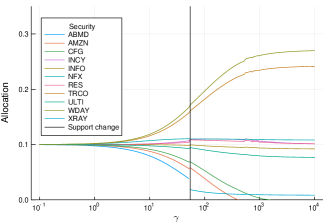
Figure 2: Sensitivity to $\gamma$ for the Russell $1000$ with $\kappa=1$ and $k=10$. The optimal security indices $\bm{z}^{\star}$ changed once over the entire range of $\gamma$.

Our final experiment studies the impact of the regularizer $\gamma$ on both solve times and the number of cuts generated, in order to justify our assertion in the introduction that increasing the amount of regularization in the problem makes the problem easier. In this direction, we solve the ten $300+$ and $400+$ instances with minimum investment and minimum return constraints studied in Section 5.2 for different values of $\gamma$ (with the copy of variables technique and in-out method on). We report the average runtime and number of cuts generated by Algorithm 3 across the $10$ instances for each $n$ in Figures 3 ($n=300$) and 4 ($n=400$).

Observe that the average runtime is essentially non-decreasing in $\gamma$, and for both $n=300$ and $n=400$ there exists a finite $\gamma>0$ at which all instances can be solved using a single cut. This empirically verifies Section 3.4’s sensitivity analysis findings.

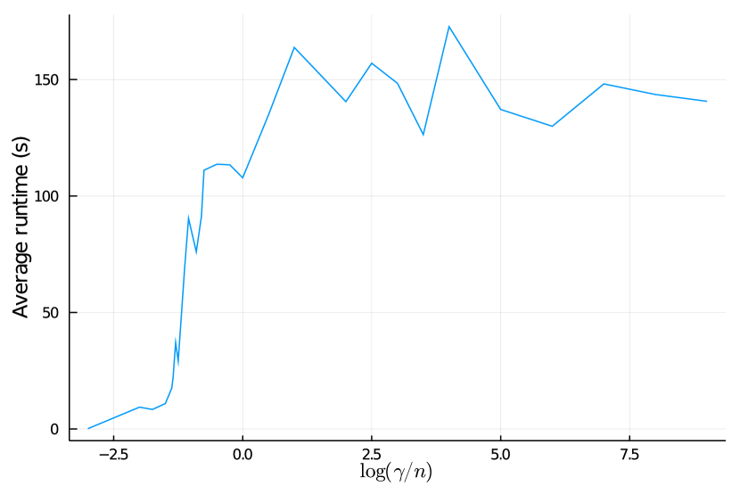
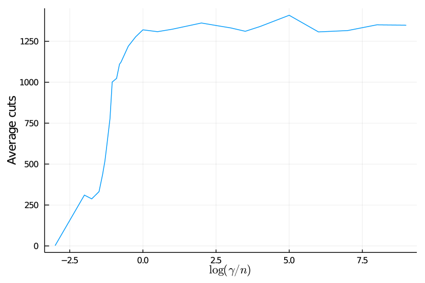
Figure 3: Average runtime (left) and number of cuts (right) vs. $\log(\gamma)$ for the $300+$ instances with buy-in and minimum return constraints with a cardinality budget of $k=10$ ($n=300$).

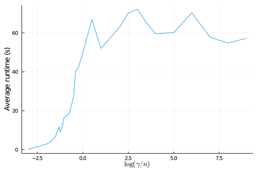
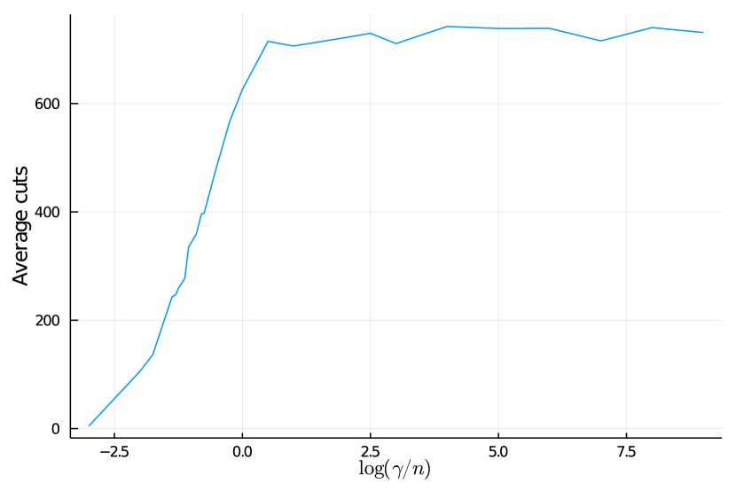
Figure 4: Average runtime (left) and number of cuts (right) vs. $\log(\gamma)$ for the $400+$ instances with buy-in and minimum return constraints with a cardinality budget of $k=10$ ($n=400$).

5.5 Summary of Findings From Numerical Experiments

We are now in a position to answer the four questions introduced at the start of this section. Our findings are as follows:

1. In the absence of complicating constraints, Algorithm 3 is substantially more efficient than commercial MIQO solvers such as CPLEX. This efficiency improvement can be explained by (a) our ability to generate stronger and more informative lower bounds via dual subproblems, and (b) our dual representation of the problems’ subgradients. Indeed, the method did not require more than one second to solve any of the constraint-free problems considered here, although this phenomenon can be partially attributed to the problem data used. Moreover, the solve times are comparable to those reported by other recent methods such as Zheng et al. (2014), Frangioni et al. (2016, 2017); note that this comparison is imperfect since the cited approaches were run on different machines and their source code is unavailable, which precludes a truly fair comparison.

2. Although imposing complicating constraints, such as minimum investment constraints, slows Algorithm 3, the method performs competitively in the presence of these constraints. Moreover, running the in-out cutting-plane method at the root node substantially reduces the initial bound gap, and allows the method to supply a certifiably near-optimal (if not optimal) solution in seconds. This suggests that running the in-out method at the root node should be considered as a viable and more scalable alternative to existing root node techniques, particularly in the presence of complicating constraints such as minimum investment constraints, or if the cardinality budget is at least $10$ (although it can do more harm than good for easier problems).

3. Algorithm 3 scales to solve real-world problem instances which comprise selecting assets from universes with thousands of securities, such as the Russell $1000$ and the Wilshire $5000$, while existing commercial solvers such as CPLEX either solve these problems much more slowly or do not successfully solve them, because they cannot attain sufficiently strong lower bounds quickly.

4. Solutions to Problem (4) are stable with respect to the hyperparameter $\gamma$.

6 Omitted Proofs

In this section, we supply the omitted proofs of results stated in the manuscript, in the order in which the results were stated.

6.1 Proof of Corollary 3.7

Proof 6.1

Proof of Corollary 3.7 This result is a simple consequence of the subgradient inequality for convex functions (see, e.g., Boyd and Vandenberghe 2004). For completeness, we now provide a proof from first principles:

The result follows from applying the lower approximation

$$f(\hat{\bm{z}})\geq f(\bm{z})+\bm{g}_{\bm{z}}^{\top}(\bm{\hat{z}}-\bm{z}),$$

re-arranging to yield

$$f(\bm{z})-f(\bm{\hat{z}})\leq-\bm{g}_{\bm{z}}^{\top}(\bm{\hat{z}}-\bm{z})$$

and invoking Corollary 3.6 to rewrite the right-hand-side in the desired form.

6.2 Proof of Corollary 4.4

Proof 6.2

Proof of Corollary 4.4 Let there exist some $(\bm{v}^{\star},\bm{w}^{\star},\bm{\alpha}^{\star},\bm{\beta}_{l}^{\star},\bm{\beta}_{u}^{\star},\lambda^{\star})$ which solve Problem (26), and binary vector $\bm{z}\in\mathcal{Z}_{k}^{n}$, such that these two quantities collectively satisfy the conditions encapsulated in Expression (29). Then, this optimal solution to Problem (26) provides the following lower bound for Problem (4):

$$-\frac{1}{2}\bm{\alpha}^{*\top}\bm{\alpha^{\star}}+\bm{y}^{\top}\bm{\alpha^{\star}}+\bm{\beta}_{l}^{*\top}\bm{l}-\bm{\beta}_{u}^{*\top}\bm{u}+\lambda^{\star}-\bm{e}^{\top}\bm{v^{\star}}-kt^{\star}.$$

Moreover, let $\bm{\hat{x}}$ be a candidate solution to Problem (4) defined by $\hat{x}_{i}:=\gamma w_{i}z_{i}$. Then, $\bm{\hat{x}}$ is feasible for Problem (4), since $\bm{l}\leq A\bm{\hat{x}}\leq\bm{u}$, $\bm{e}^{\top}\hat{\bm{x}}=1$, $\bm{\hat{x}}\geq\bm{0}$ and $\|\hat{\bm{x}}\|_{0}\leq k$ by Expression (29) and the definition of $\bm{z}$. Additionally, since an optimal choice of $t$ is the $k$th largest value of $\frac{\gamma}{2}w_{i}^{2}$, i.e., $\frac{\gamma}{2}w_{[k]}^{2}$ (see Zakeri et al. 2014, Lemma 1), at optimality we have that $\bm{e}^{\top}\bm{v}+kt=\frac{1}{2\gamma}\hat{\bm{x}}^{\top}\hat{\bm{x}}$. Therefore, Problem (4)’s objective when $\bm{x}=\hat{\bm{x}}$ is given by:

$$-\frac{1}{2}\bm{\alpha}^{*\top}\bm{\alpha^{\star}}+\bm{y}^{\top}\bm{\alpha^{\star}}+\bm{\beta}_{l}^{*\top}\bm{l}-\bm{\beta}_{u}^{*\top}\bm{u}+\lambda^{\star}-\frac{1}{2\gamma}\bm{\hat{x}}^{\top}\bm{\hat{x}},$$

which is less than or equal to Problem (26)’s objective, since $v_{i}^{\star}=0\quad\forall i\in[n]\ :\ z_{i}=0$.

Finally, let $|w^{\star}|_{[k]}>|w^{\star}|_{[k+1]}$ and let $S$ denote the set of indices such that $|w^{\star}_{i}|\geq|w^{\star}|_{[k]}$. Then, as the primal-dual KKT conditions for max-$k$ norms (see, e.g., Zakeri et al. 2014, Lemma 1) imply that an optimal choice of $t$ is given by $t^{\star}=\frac{\gamma}{2}w^{\star 2}_{[k]}$, we can set $t^{\star}=\frac{\gamma}{2}w^{\star 2}_{[k]}$ without loss of generality. Note that, in general, this choice is not unique. Indeed, any $t\in[\frac{\gamma}{2}w_{[k+1]}^{\star},\frac{\gamma}{2}w_{[k]}^{\star}]$ constitutes an optimal choice (Zakeri et al. 2014).

We then have that $v_{i}^{\star}=0\forall i\notin S$, which implies that the constraint $v_{i}+t\geq\frac{\gamma}{2}w_{i}^{2}$ holds strictly for any $i\notin S$. Therefore, the dual multipliers associated with these constraints must take value $0$. But these constraints’ dual multipliers are precisely $\bm{z}\in\mathrm{Conv}(\mathcal{Z}_{k}^{n})$, which implies that $z_{i}=1\forall i\in S$ gives a valid set of dual multipliers. Moreover, by Equation (12), setting $\bm{x}_{i}=\gamma z_{i}w_{i}^{\star}$ supplies an optimal (and thus feasible) choice of $\bm{x}$ for this fixed $\bm{z}$. Therefore, this primal-dual pair satisfies (29).

7 Supplementary Experimental Results

7.1 Supplementary Results on Problems With Minimum Investment Constraints

We now present the instance-wise runtimes (in seconds) for all instances generated by Frangioni and Gentile (2006), in Tables 10-12.

Table 10: Performance of the outer-approximation method vs. CPLEX’s MISOCO method on the $200^{+}$ instances generated by Frangioni and Gentile (2006), with a time budget of $600$s per approach, $\kappa=0$, $\gamma=\frac{1000}{n}$. We run all approaches on one thread. Note that “nc” refers to an instance without an explicit cardinality constraint.

Problem	$k$	Algorithm 3			Algorithm 3 $+$ in-out			Algorithm 3 $+$ in-out $+$ 50			CPLEX MISOCO
		Time	Nodes	Cuts	Time	Nodes	Cuts	Time	Nodes	Cuts	Time	Nodes
pard200-1	6	0.74	674	126	1.61	832	162	10.80	248	36	28.54	33
pard200-1	8	1.10	1,038	188	2.00	1,140	220	12.95	488	60	30.63	33
pard200-1	10	8.73	8,844	654	8.58	6,582	494	12.44	2,838	180	65.04	69
pard200-1	12	1.37	1,902	136	1.05	1,079	74	7.84	532	29	130.9	122
pard200-1	nc	1.66	3,026	123	1.58	1,182	101	9.68	928	79	$>600$	624
pard200-2	6	0.13	141	24	0.16	81	10	3.21	42	5	33.26	37
pard200-2	8	0.36	327	59	0.28	117	23	5.19	64	11	35.90	29
pard200-2	10	4.19	6,313	317	4.07	4,449	243	10.62	2,530	144	278.6	331
pard200-2	12	0.65	1,953	20	0.42	187	8	7.94	182	7	$>600$	775
pard200-2	nc	0.7	1,716	24	0.53	233	11	7.37	184	10	$>600$	800
pard200-3	6	0.87	904	158	0.81	740	96	6.55	413	40	103.7	103
pard200-3	8	0.67	818	98	0.82	671	84	6.54	343	40	85.76	81
pard200-3	10	2.45	4,584	189	1.45	1,444	90	8.28	840	42	210.9	215
pard200-3	12	1.71	3,034	42	0.78	923	23	7.75	461	9	$>600$	648
pard200-3	nc	1.21	2,803	38	0.65	781	21	8.68	416	9	$>600$	688
pard200-4	6	1.53	2,096	262	2.31	1,740	227	8.34	1,529	193	230.3	248
pard200-4	8	2.73	3,820	343	2.82	3,055	260	9.50	1,740	139	176.1	194
pard200-4	10	10.83	14,200	647	10.82	11,380	522	17.9	7,912	446	527.5	617
pard200-4	12	0.98	2,332	22	0.32	272	12	7.83	226	11	581.4	643
pard200-4	nc	0.86	2,315	22	0.39	251	12	7.65	206	11	592.7	648
pard200-5	6	0.44	225	79	0.41	147	49	5.06	69	15	33.6	31
pard200-5	8	0.66	407	112	0.53	253	65	5.71	93	16	36.0	34
pard200-5	10	2.86	3,577	322	1.76	1,644	149	7.62	453	48	84.98	79
pard200-5	12	135.9	171,500	722	12.13	10,700	294	18.45	6,098	171	$>600$	686
pard200-5	nc	120.4	131,100	777	15.16	11,960	285	17.06	5,866	142	$>600$	818
pard200-6	6	7.15	4,635	933	7.44	5,148	902	16.1	4,875	675	172.2	199
pard200-6	8	6.05	5,985	777	8.38	5,885	733	12.25	4,120	349	112.6	135
pard200-6	10	2.64	2,305	283	2.05	1,172	206	7.48	514	107	82.61	103
pard200-6	12	1.08	1,934	81	0.54	461	37	7.18	409	23	189.0	211
pard200-6	nc	1.1	1,737	76	0.74	799	48	8.22	483	32	$>600$	700
pard200-7	6	0.64	687	122	0.74	602	97	6.77	291	54	112.7	119
pard200-7	8	0.36	431	59	0.32	207	31	7.12	88	16	59.57	65
pard200-7	10	2.21	3,570	216	1.15	1,205	105	8.13	640	46	83.51	75
pard200-7	12	12.03	15,000	76	1.17	1,185	20	9.17	725	13	$>600$	648
pard200-7	nc	8.77	12,930	72	1.32	1,464	23	9.39	841	16	$>600$	802
pard200-8	6	0.2	97	43	0.19	75	25	2.57	41	11	20.55	19
pard200-8	8	0.36	199	68	0.51	124	36	3.37	47	12	32.90	30
pard200-8	10	3.21	3,635	295	0.78	442	88	7.26	151	20	40.55	37
pard200-8	12	96.29	82,400	581	3.09	2,237	171	8.71	1,080	56	185.2	200
pard200-8	nc	45.68	66,790	574	2.96	2,455	160	10.21	1,999	67	$>600$	964
pard200-9	6	2.6	2,404	390	2.62	2,262	338	7.75	1,211	110	79.61	91
pard200-9	8	5.62	5,052	657	5.83	3,814	540	10.19	2,093	289	108.1	136
pard200-9	10	3.76	3,582	403	3.09	1,817	259	9.53	754	125	65.21	82
pard200-9	12	1.98	2,535	147	0.52	296	42	7.76	134	10	23.70	23
pard200-9	nc	1.96	2,473	148	1.65	1,675	95	9.89	899	78	$>600$	675
pard200-10	6	1.2	1,122	226	1.42	992	188	6.86	385	41	63.01	73
pard200-10	8	1.62	1,599	242	1.48	992	178	6.91	415	41	56.54	61
pard200-10	10	36.51	25,450	1,771	9.51	6,730	833	14.27	4,025	597	178.0	232
pard200-10	12	3.8	5,711	211	0.58	300	35	7.78	152	10	20.48	25
pard200-10	nc	4.75	7,010	230	2.93	2,085	164	11.84	2115	117	$>600$	632

Table 11: Performance of the outer-approximation method vs. CPLEX’s MISOCO method on the $300^{+}$ instances generated by Frangioni and Gentile (2006), with a time budget of $600$s per approach, with $\kappa=0$, $\gamma=\frac{1000}{n}$. We run all approaches on one thread. Note that “nc” refers to an instance without an explicit cardinality constraint.

Problem	$k$	Algorithm 3			Algorithm 3 $+$ in-out			Algorithm 3 $+$ in-out $+$ 50			CPLEX MISOCO
		Time	Nodes	Cuts	Time	Nodes	Cuts	Time	Nodes	Cuts	Time	Nodes
pard300-1	6	36.56	15,870	1,974	68.44	14,130	1,864	67.68	10,920	1,295	$>600$	210
pard300-1	8	158.8	39,650	3,412	238.9	37,830	3,320	193.8	29,560	2,508	$>600$	190
pard300-1	10	108.3	60,560	2,593	94.63	46,350	2,053	59.74	23,270	1,243	$>600$	230
pard300-1	12	17.93	17,070	523	8.23	5,390	219	16.30	1,567	73	261.3	101
pard300-1	nc	33.85	29,030	483	26.44	15,490	419	44.41	15,060	418	$>600$	206
pard300-2	6	13.87	7,583	935	22.34	6,805	819	28.03	4,563	496	346.5	117
pard300-2	8	37.76	28,910	1,962	68.53	21,470	1,753	66.81	16,060	1,254	583.0	233
pard300-2	10	64.51	41,320	2,247	44.76	30,230	1,237	439.9	15,460	658	562.7	216
pard300-2	12	2.76	4,355	115	0.77	532	26	12.22	194	4	172.3	57
pard300-2	nc	4.91	7,423	123	1.91	1,440	63	13.29	739	38	$>600$	250
pard300-3	6	33.24	21,540	1,205	47.62	20,050	1,137	52.85	13,420	793	$>600$	210
pard300-3	8	34.00	37,920	1,410	52.85	35,640	1,293	38.12	21,620	668	$>600$	206
pard300-3	10	254.3	128,500	3,526	283.2	103,700	3,114	288.0	112,000	2,502	$>600$	210
pard300-3	12	81.05	59,470	342	4.5	3,607	84	18.83	1,144	47	$>600$	295
pard300-3	nc	77.34	58,550	328	8.26	5,867	116	25.16	5,137	74	$>600$	206
pard300-4	6	51.46	18,810	2,255	55.49	18,400	1,849	64.77	15,930	1,539	$>600$	225
pard300-4	8	75.72	39,830	3,192	161.3	45,040	3,108	154.5	36,930	2,611	$>600$	224
pard300-4	10	168.0	58,710	3,968	195.2	58,490	3,672	168.2	44,360	3,048	$>600$	238
pard300-4	12	19.98	18,650	267	8.93	5,509	187	22.75	3,707	127	$>600$	229
pard300-4	nc	27.19	22,010	284	16.06	12,240	215	31.03	9,941	199	$>600$	257
pard300-5	6	3.99	2,670	425	5.49	2,295	351	12.05	934	104	358.1	131
pard300-5	8	6.88	5,509	491	6.53	4,227	357	11.90	1,100	73	192.5	68
pard300-5	10	13.5	11,890	790	6.86	4,610	385	14.23	1,419	140	330.3	123
pard300-5	12	1.07	1,141	81	0.43	174	30	10.71	120	18	247.7	92
pard300-5	nc	1.05	813	82	1.03	511	50	12.24	360	31	$>600$	224
pard300-6	6	3.66	2,478	420	4.00	2,341	353	11.47	1,089	101	155.5	55
pard300-6	8	10.35	8,220	771	9.71	6,503	635	15.40	3,518	295	307.6	110
pard300-6	10	26.95	15,450	1,151	19.09	12,090	927	21.74	6,265	402	$>600$	209
pard300-6	12	6.62	7,094	275	3.74	1,118	136	19.10	794	79	121.4	47
pard300-6	nc	7.65	9,391	257	5.17	3,233	195	19.06	3,056	158	$>600$	214
pard300-7	6	2.82	2,009	323	3.89	1,413	285	12.86	1,120	195	551.5	227
pard300-7	8	4.08	4,395	337	3.3	1,996	250	13.68	1,182	168	$>600$	210
pard300-7	10	5.08	5,494	334	1.77	1,716	107	11.13	464	26	199.0	63
pard300-7	12	0.71	1,278	37	0.56	455	18	11.94	373	14	577.8	208
pard300-7	nc	1.43	2,940	37	0.59	615	13	11.53	374	12	$>600$	200
pard300-8	6	5.28	3,174	589	6.05	3,052	549	13.53	2,232	282	331.9	113
pard300-8	8	11.74	7,725	1,034	15.13	7,912	983	20.73	5,125	658	523.2	185
pard300-8	10	23.65	18,550	1,174	12.02	8,273	602	18.47	3,646	354	368.3	130
pard300-8	12	7.02	8,034	331	4.33	2,786	171	14.83	1,447	104	234.7	89
pard300-8	nc	8.88	9,420	333	7.09	6,558	287	19.36	4,719	239	$>600$	220
pard300-9	6	12.26	13,400	1,033	15.08	8,177	931	20.94	4,948	620	538.5	195
pard300-9	8	97.90	31,670	2,356	76.99	30,940	2,192	77.93	24,080	1,823	$>600$	207
pard300-9	10	215.2	97,800	2,741	118.1	64,980	1,907	66.37	36,790	1,113	$>600$	201
pard300-9	12	11.08	11,750	268	9.68	8,423	196	18.18	3,710	117	$>600$	269
pard300-9	nc	24.51	25,400	284	10.65	8,604	225	31.34	10,640	196	$>600$	240
pard300-10	6	5.13	3,884	583	7.5	3,589	503	15.05	2,227	234	262.5	93
pard300-10	8	9.54	6,685	803	11.44	5,257	687	17.12	3,190	300	289.0	107
pard300-10	10	6.02	3,417	486	4.96	2,097	380	14.25	1,215	229	259.5	99
pard300-10	12	13.33	9,969	388	5.35	3,815	207	14.56	1,690	84	$>600$	195
pard300-10	nc	26.77	16,430	410	15.2	8,326	336	35.89	9,676	319	$>600$	175

Table 12: Performance of the outer-approximation method vs. CPLEX’s MISOCO method on the $400^{+}$ instances generated by Frangioni and Gentile (2006), with a time budget of $600$s per approach, with $\kappa=0$, $\gamma=\frac{1000}{n}$. We run all approaches on one thread. Note that “nc” refers to an instance without an explicit cardinality constraint.

Problem	$k$	Algorithm 3			Algorithm 3 $+$ in-out			Algorithm 3 $+$ in-out $+$ 50			CPLEX MISOCO
		Time	Nodes	Cuts	Time	Nodes	Cuts	Time	Nodes	Cuts	Time	Nodes
pard400-1	6	64.88	18,730	2,963	69.91	17,430	2,670	86.00	17,793	2,320	$>600$	95
pard400-1	8	364.5	54,420	5,400	283.6	66,130	4,734	232.7	41,000	4,086	$>600$	94
pard400-1	10	36.33	24,850	980	13.25	8,578	554	24.45	3,740	318	$>600$	97
pard400-1	12	14.19	11,480	328	9.40	6,732	214	24.06	4,030	144	$>600$	100
pard400-1	nc	49.56	35,030	336	17.41	11,580	261	44.27	16,000	238	$>600$	74
pard400-2	6	0.18	71	21	0.12	24	8	3.31	18	6	160.9	17
pard400-2	8	0.31	227	24	0.13	12	8	2.17	14	8	350.9	53
pard400-2	10	0.14	87	10	0.05	0	2	0.05	0	2	178.2	23
pard400-2	12	0.12	54	6	0.24	10	3	1.13	5	3	$>600$	69
pard400-2	nc	0.12	52	5	0.25	9	2	2.57	12	2	$>600$	70
pard400-3	6	1.38	1,335	149	1.70	895	121	16.37	534	84	$>600$	100
pard400-3	8	3.22	2,458	271	3.24	1,862	206	18.40	1,353	133	$>600$	80
pard400-3	10	8.81	9,924	347	3.22	2,500	146	19.15	1,351	55	$>600$	82
pard400-3	12	0.45	838	12	0.26	102	2	13.71	59	2	582.0	92
pard400-3	nc	0.56	1,259	10	0.22	130	2	15.34	74	2	$>600$	100
pard400-4	6	53.04	18,490	1,712	54.56	14,360	1,677	57.55	10,890	1,237	$>600$	99
pard400-4	8	183.9	47,460	3,660	179.0	42,140	3,522	166.1	37,070	2,923	$>600$	90
pard400-4	10	259.1	76,390	2,153	516.5	81,900	5,782	439.3	96,750	3,614	$>600$	90
pard400-4	12	1.88	2,428	98	0.64	311	21	15.56	220	12	407.6	67
pard400-4	nc	3.76	4,738	105	2.14	1,795	66	18.33	1,008	53	$>600$	90
pard400-5	6	11.07	5,100	658	11.41	4,793	586	23.78	3,363	363	$>600$	94
pard400-5	8	17.42	12,060	939	20.97	9,459	811	35.33	6,300	507	$>600$	94
pard400-5	10	213.7	74,590	2,312	175.9	73,740	1,933	100.6	42,380	1,184	$>600$	89
pard400-5	12	9.29	9,720	272	4.13	2,538	105	19.9	765	59	485.4	95
pard400-5	nc	17.16	15,750	306	19.33	12,320	235	38.46	9,137	244	$>600$	70
pard400-6	6	0.27	116	30	0.25	32	9	6.34	37	6	356.2	61
pard400-6	8	0.17	92	15	0.06	0	2	0.08	0	2	208.4	33
pard400-6	10	0.42	317	36	0.18	44	9	4.81	18	2	200.9	33
pard400-6	12	4.8	7,491	76	0.91	545	22	19.21	324	15	$>600$	97
pard400-6	nc	5.4	8,154	82	1.36	654	17	19.44	372	15	$>600$	83
pard400-7	6	48.05	16,100	2,514	90.72	12,480	2,376	122.5	14,130	2,233	$>600$	98
pard400-7	8	114.0	39,650	3,412	178.3	30,110	3,224	194.2	27,800	2,819	$>600$	86
pard400-7	10	31.51	21,060	1,304	35.49	19,670	985	32.94	8,230	497	$>600$	86
pard400-7	12	1.38	1,567	70	0.42	164	13	12.63	60	5	169.5	25
pard400-7	nc	1.77	2,063	83	2.09	1,410	64	17.73	893	42	$>600$	61
pard400-8	6	118.1	27,150	3,187	165.0	28,200	3,025	185.1	24,550	2,753	$>600$	98
pard400-8	8	342.8	91,060	5,120	335.7	62,250	5,377	356.2	58,570	4,889	$>600$	97
pard400-8	10	229.3	113,200	2,704	105.9	60,640	1,546	86.51	36,100	1,100	$>600$	91
pard400-8	12	3.14	3,999	100	1.31	948	31	19.45	248	16	375.6	55
pard400-8	nc	3.14	3,717	92	4.26	3,786	78	22.05	1,974	63	$>600$	57
pard400-9	6	77.79	22,580	2,345	103.5	20,500	2,242	107.7	17,480	1,788	$>600$	88
pard400-9	8	466.0	60,570	4,064	227.1	63,950	3,900	217.7	54,390	3,298	$>600$	89
pard400-9	10	409.0	126,200	3,610	16.71	8,440	448	34.38	6,406	315	$>600$	77
pard400-9	12	0.69	747	52	0.72	238	33	14.43	212	20	$>600$	96
pard400-9	nc	0.61	629	43	0.77	458	33	14.5	379	22	$>600$	100
pard400-10	6	170.0	23,610	3,587	168.1	22,860	3,473	227.1	21,270	3,172	$>600$	90
pard400-10	8	245.2	45,870	5,375	380.3	53,370	5,307	410.4	53,740	4,974	$>600$	92
pard400-10	10	391.6	108,400	3,236	177.5	67,620	2,292	72.6	26,350	1,162	$>600$	80
pard400-10	12	3.79	4,910	152	1.01	557	42	16.65	351	22	360.0	57
pard400-10	nc	4.70	4,035	143	4.08	3253	130	20.43	2,239	113	$>600$	37

We now present the instance-wise runtimes (in seconds) for the smallest instances generated by Frangioni and Gentile (2006), without any diagonal matrix extraction, and $k\in\{6,8,10,12,n\}$. Table 13 demonstrates that not using any diagonal matrix extraction technique substantially slows our approach.

Table 13: Performance of the outer-approximation method on the $200^{+}$ instances generated by Frangioni and Gentile (2006), with a time budget of $600$s per approach, $\kappa=0$, $\gamma=\frac{1000}{n}$, and no diagonal matrix extraction. We run all approaches on one thread. Note that “nc” refers to an instance without an explicit cardinality constraint.

Problem	$k$	Algorithm 3			Algorithm 3$+$in-out			Algorithm 3 $+$ in-out $+$ 50			CPLEX MISOCO
		Time	Nodes	Cuts	Time	Nodes	Cuts	Time	Nodes	Cuts	Time	Nodes
pard200-1	6	$>600$	143,800	10,650	$>600$	217,200	9,671	$>600$	120,900	7,530	$>600$	700
pard200-1	8	$>600$	94,900	11,830	400.6	118,300	6,461	$>600$	106,900	7,822	$>600$	600
pard200-1	10	$>600$	173,000	10,020	$>600$	71,050	10,340	$>600$	63,470	5,422	$>600$	700
pard200-1	12	$>600$	223,700	6,852	$>600$	68,600	10,500	$>600$	42,450	6,632	$>600$	686
pard200-1	nc	$>600$	286,600	8,236	$>600$	59,070	12,560	$>600$	53,580	8,221	$>600$	800
pard200-2	6	$>600$	243,600	10,930	239.9	47,180	8,305	$>600$	90,460	8,538	$>600$	500
pard200-2	8	$>600$	328,100	9,365	$>600$	234,100	8,547	$>600$	207,800	2,011	$>600$	242
pard200-2	10	$>600$	468,400	9,134	0.2	47	12	5.32	28	16	$>600$	700
pard200-2	12	$>600$	273,300	7,406	0.47	3	18	1.12	3	18	$>600$	700
pard200-2	nc	$>600$	505,000	8,497	0.21	65	12	9.95	69	12	$>600$	600
pard200-3	6	$>600$	112,800	12,020	1.36	236	32	43.69	515	32	$>600$	505
pard200-3	8	$>600$	235,000	10,150	1.24	385	24	59.49	750	24	$>600$	500
pard200-3	10	$>600$	245,500	6,940	3.56	6,937	12	136.5	44,310	18	$>600$	510
pard200-3	12	$>600$	292,360	7,016	57.13	63,850	944	$>600$	139,800	935	$>600$	346
pard200-3	nc	$>600$	334,300	8,382	42.01	77,870	2,384	285.73	120,900	3,660	$>600$	600
pard200-4	6	$>600$	86,780	13,660	0.3	0	14	0.49	0	14	$>600$	500
pard200-4	8	$>600$	272,600	10,700	0.4	642	20	50.41	620	20	$>600$	561
pard200-4	10	$>600$	289,900	8,193	0.61	516	30	46.85	879	32	$>600$	498
pard200-4	12	$>600$	303,600	6,790	0.9	228	16	51.31	216	16	$>600$	294
pard200-4	nc	$>600$	366,100	7,999	0.38	86	22	13.87	80	22	$>600$	587
pard200-5	6	$>600$	112,000	9,616	$>600$	141,200	9,208	$>600$	127,100	7,060	$>600$	700
pard200-5	8	$>600$	132,600	11,370	135.0	52,970	4,089	$>600$	93,390	7,365	$>600$	600
pard200-5	10	$>600$	183,100	9,788	$>600$	51,300	10,010	$>600$	68,410	6,456	$>600$	700
pard200-5	12	$>600$	203,500	5,519	$>600$	53,730	9,813	$>600$	39,300	5,365	$>600$	600
pard200-5	nc	$>600$	315,400	9,270	$>600$	59,070	12,680	$>600$	86,240	7,025	$>600$	800
pard200-6	6	$>600$	116,700	11,260	$>600$	181,500	8,698	$>600$	131,200	6,758	$>600$	691
pard200-6	8	$>600$	161,100	10,700	$>600$	202,060	9,698	$>600$	105,400	8,449	$>600$	700
pard200-6	10	$>600$	141,200	11,370	$>600$	80,800	11,170	$>600$	56,700	7,828	$>600$	700
pard200-6	12	$>600$	236,600	7,586	$>600$	52,560	11,000	$>600$	41,630	5,415	$>600$	400
pard200-6	nc	$>600$	338,100	9,120	$>600$	71,790	13,850	$>600$	50,980	8,922	$>600$	800
pard200-7	6	$>600$	106,000	8,527	3.66	4,736	392	72.66	6,080	391	$>600$	500
pard200-7	8	$>600$	149,800	12,640	$>600$	193,900	10,840	$>600$	222,800	3,503	$>600$	500
pard200-7	10	$>600$	214,200	9,858	$>600$	139,000	8,465	$>600$	154,300	5,859	$>600$	485
pard200-7	12	$>600$	313,000	7,902	$>600$	206,900	9,568	$>600$	215,100	3,773	$>600$	500
pard200-7	nc	$>600$	220,800	6,976	$>600$	194,500	8,507	$>600$	209,600	4,971	$>600$	700
pard200-8	6	$>600$	167,600	11,200	$>600$	217,700	9,307	$>600$	173,200	7,609	$>600$	650
pard200-8	8	$>600$	183,200	11,140	$>600$	213,900	10,100	$>600$	103,100	5,954	$>600$	700
pard200-8	10	$>600$	182,400	10,190	$>600$	115,600	9,215	$>600$	35,700	4,307	$>600$	360
pard200-8	12	$>600$	217,000	6,149	$>600$	52,420	10,550	$>600$	52,300	9,066	$>600$	700
pard200-8	nc	$>600$	241,600	6,751	$>600$	56,070	11,820	$>600$	50,590	7,702	$>600$	471
pard200-9	6	$>600$	126,500	11,140	$>600$	128,500	9,437	$>600$	106,200	7,029	$>600$	600
pard200-9	8	$>600$	130,300	10,580	$>600$	135,700	8,579	$>600$	88,600	6,653	$>600$	700
pard200-9	10	$>600$	186,500	11,160	$>600$	63,560	10,570	$>600$	57,800	5,646	$>600$	600
pard200-9	12	$>600$	266,100	7,433	$>600$	61,000	10,700	$>600$	42,550	6,381	$>600$	689
pard200-9	nc	$>600$	256,100	7,535	$>600$	57,280	10,540	$>600$	38,560	6,376	$>600$	800
pard200-10	6	$>600$	179,600	12,700	$>600$	245,900	7,980	$>600$	155,100	7,300	$>600$	600
pard200-10	8	$>600$	123,600	10,060	$>600$	198,370	8,670	$>600$	36,770	2,414	$>600$	680
pard200-10	10	$>600$	164,800	8,273	$>600$	46,100	9,375	$>600$	29,000	4,824	$>600$	393
pard200-10	12	$>600$	193,300	5,776	$>600$	52,820	9,616	$>600$	37,900	5,834	$>600$	364
pard200-10	nc	$>600$	193,700	5,523	$>600$	40,770	8,887	$>600$	34,300	6,096	$>600$	432

Next, we present the aggregate runtimes (in seconds) for all instances generated by Frangioni and Gentile (2006), when we run CPLEX’s MISOCP solver after first supplying the cuts generated by the in-out method. Note that, to allow CPLEX to benefit from the in-out cuts, we introduce an auxiliary variable $\tau$, change the objective to minimizing $\tau$, impose the constraint $\tau\geq\frac{1}{2}\bm{x}^{\top}\bm{\Sigma}\bm{x}+\frac{1}{2\gamma}\bm{e}^{\top}\bm{\theta}-\kappa\bm{mu}^{\top}\bm{x}$ to model the MISOCO objective, and impose the cuts from the in-out method using the epigraph variable $\tau$.

Table 14: Average runtime in seconds per approach with $\kappa=0$, $\gamma=\frac{1000}{n}$ for the problems generated by Frangioni and Gentile (2006). We impose a time limit of $600$s and run all approaches on one thread. If a solver fails to converge, we report the number of explored nodes at the time limit, use $600$s in lieu of the solve time, and report the number of failed instances (out of $10$) next to the solve time in brackets. Note that the minimum investment constraints impose an implicit cardinality constraint with $k\approx{\color[rgb]{0,0,0}13}$.

Problem	$k$	CPLEX MISOCO in-out
		Time	Nodes
200+	6	255.5 (1)	92.3
200+	8	272.2 (1)	98.4
200+	10	375.2 (3)	116.4
200+	12	447.8 (6)	216
200+	200	$>600$ (10)	332.1
300+	6	573.4 (9)	92
300+	8	578.4 (9)	89.2
300+	10	$>600$ (10)	92.1
300+	12	575.65 (9)	117.3
300+	200	$>600$ (10)	108.5
400+	6	569.4 (9)	43.3
400+	8	563.3 (9)	45.1
400+	10	562.4 (9)	45.7
400+	12	593.8 (9)	58.3
400+	200	$>600$ (10)	41.4

Finally, we present the instance-wise runtimes (in seconds) for the smallest instances generated by Frangioni and Gentile (2006), with the diagonal matrix extraction technique proposed by Zheng et al. (2014), and $k\in\{10,n\}$ (we restrict the values $k$ can take to use the diagonal matrices pre-computed by Frangioni et al. (2017)). Table 15 demonstrates that using the diagonal matrix extraction technique proposed by Zheng et al. (2014) substantially slows our approach; the results for $n\in\{300,400\}$ are similar. Indeed, this technique is only faster for the pard$200$-$1$ problem with $k=10$, and is slower in the other $95\%$ of instances (sometimes substantially so).

Table 15: Performance of the outer-approximation method on the $200^{+}$ instances generated by Frangioni and Gentile (2006), with a time budget of $600$s per approach, $\kappa=0$, $\gamma=\frac{1000}{n}$, and the diagonal matrix extraction technique proposed by Zheng et al. (2014). We run all approaches on one thread. Note that “nc” refers to an instance without an explicit cardinality constraint.

Problem	$k$	Algorithm 3			Algorithm 3 $+$ in-out			Algorithm 3 $+$ in-out $+$ 50
		Time	Nodes	Cuts	Time	Nodes	Cuts	Time	Nodes	Cuts
pard200-1	10	0.74	130	30	0.03	0	4	0.03	0	4
pard200-1	nc	$>600$	887,400	1,386	$>600$	539,900	1,070	$>600$	369,500	675
pard200-2	10	234.3	239,500	875	57.14	45,230	193	78.88	39,000	196
pard200-2	nc	$>600$	995,900	823	$>600$	157,100	135	$>600$	226,100	66
pard200-3	10	245.1	207,200	1,195	71.95	55,050	365	76.64	30,910	249
pard200-3	nc	$>600$	903,500	888	$>600$	357,200	246	$>600$	268,400	259
pard200-4	10	$>600$	442,500	1,967	344.7	223,700	1,053	228.9	135,500	760
pard200-4	nc	535.1	913,500	1,092	$>600$	297,600	94	529.8	212,600	94
pard200-5	10	$>600$	439,900	4,965	48.87	70,200	206	69.71	52,300	204
pard200-5	nc	$>600$	1,340,000	1,314	$>600$	531,400	1,408	$>600$	573,200	1,358
pard200-6	10	$>600$	311,800	4,922	6.54	6,382	116	36.29	12,370	107
pard200-6	nc	$>600$	1,280,000	1,016	$>600$	479,900	789	$>600$	557,600	580
pard200-7	10	549.8	389,000	2,542	515.6	228,100	1,336	292.4	105,900	743
pard200-7	nc	$>600$	1,245,000	522	$>600$	496,200	183	$>600$	502,600	119
pard200-8	10	$>600$	399,200	3,419	2.32	1,638	46	20.19	1,716	45
pard200-8	nc	$>600$	1,337,000	862	$>600$	674,300	552	$>600$	507,900	420
pard200-9	10	589.7	576,100	1,756	6.31	8,746	122	26.53	8,290	143
pard200-9	nc	$>600$	1,264,000	1,941	$>600$	703,900	1,977	$>600$	498,000	1,970
pard200-10	10	$>600$	416,200	3,798	288.4	160,300	1,070	422.0	192,800	1,002
pard200-10	nc	$>600$	974,400	1,584	$>600$	498,100	1,513	$>600$	313,400	1482

8 Additional Pseudocode

In this appendix, we provide auxiliary pseudocode pertaining to the experiments run in Section 5. Specifically, we provide pseudocode pertaining to our implementation of the in-out method of Ben-Ameur and Neto (2007), which we have applied before running Algorithm 3 in some problems in Section 5.

Algorithm 4 The in-out method of Ben-Ameur and Neto (2007), as applied at the root node.

0:  Optimal solution to Problem (27) $\bm{z}^{\star}$, objective value $\theta_{\text{soco}}$

  $\epsilon\leftarrow 10^{-10},\lambda\leftarrow 0.1,\delta\leftarrow 2\epsilon$

  $t\leftarrow 1$

  repeat

     Compute $\bm{z}_{0},\theta_{0}$ solution of

$$\min_{\bm{z}\in\mathrm{Conv}\left(\mathcal{Z}_{k}^{n}\right),\theta}\>\theta\quad\mbox{ s.t. }\quad\theta\geq f(\bm{z}_{i})+g_{\bm{z}_{i}}^{\top}(\bm{z}-\bm{z}_{i})\quad\forall i\in[t].$$

     if $z_{0}$ has not improved for $5$ consecutive iterations then

        Set $\lambda=1$

        if $z_{0}$ has not improved for $10$ consecutive iterations then

           Set $\delta=0$

        end if

     end if

     Set $z_{t+1}\leftarrow\lambda z_{0}+(1-\lambda)z_{\text{soco}}+\delta\bm{e}$.

     Round $\bm{z}_{t+1}$ coordinate-wise so that $\bm{z}_{t+1}\in[0,1]^{n}$.

     Compute $f(\bm{z}_{t+1})$ and $g_{\bm{z}_{t+1}}\in\partial f(\bm{z}_{t+1})$.

     Apply cut $\theta\geq f(\bm{z}_{t+1})+g_{\bm{z}_{t+1}}^{\top}(\bm{z}-\bm{z}_{t+1})$ at root node of integer model.

     $t\leftarrow t+1$

  until $f(\bm{z}_{0})-\theta_{0}\leq\varepsilon$ or $t>200$

  return  $\bm{z}_{t}$

References

- Abadie (1967) Abadie J (1967) On the Kuhn-Tucker theorem. Nonlinear programming (North-Holland Publishing Co., Amsterdam).
- Ahmadi et al. (2017) Ahmadi AA, Dash S, Hall G (2017) Optimization over structured subsets of positive semidefinite matrices via column generation. Disc. Optim. 24:129–151.
- Aktürk et al. (2009) Aktürk MS, Atamtürk A, Gürel S (2009) A strong conic quadratic reformulation for machine-job assignment with controllable processing times. Oper. Res. Letters 37(3):187–191.
- Barker and Carlson (1975) Barker G, Carlson D (1975) Cones of diagonally dominant matrices. Pacific Journal of Mathematics 57(1):15–32.
- Beasley (1990) Beasley JE (1990) OR-library: distributing test problems by electronic mail. J. Oper. Res. Soc. 41(11):1069–1072.
- Ben-Ameur and Neto (2007) Ben-Ameur W, Neto J (2007) Acceleration of cutting-plane and column generation algorithms: Applications to network design. Networks 49(1):3–17.
- Ben-Tal and Nemirovski (2001) Ben-Tal A, Nemirovski A (2001) Lectures on modern convex optimization: Analysis, algorithms, and engineering applications, volume 2 (SIAM Philadelphia, PA).
- Benders (1962) Benders JF (1962) Partitioning procedures for solving mixed-variables programming problems. Numerische mathematik 4(1):238–252.