An unoriented skein relation
via bordered–sutured Floer homology

Abstract.

We show that the bordered–sutured Floer invariant of the complement of a tangle in an arbitrary $3$-manifold $Y$, with minimal conditions on the bordered–sutured structure, satisfies an unoriented skein exact triangle. This generalizes a theorem by Manolescu [Man07:HFKUnorientedSkein] for links in $S^{3}$. We give a theoretical proof of this result by adapting holomorphic polygon counts to the bordered–sutured setting, and also give a combinatorial description of all maps involved and explicitly compute them. We then show that, for $Y=S^{3}$, our exact triangle coincides with Manolescu’s. Finally, we provide a graded version of our result, explaining in detail the grading reduction process involved.

1. Introduction

Knot Floer homology, defined by Ozsváth and Szabó [OzsSza04:HFK], and independently by Rasmussen [Ras03:HFK], is an invariant of oriented, null-homologous knots $K$ in an oriented, connected, closed $3$-manifold $Y$. It is then extended by Ozsváth and Szabó [OzsSza08:HFL] to an invariant for oriented links $L$. The simplest flavor $\widehat{\operatorname{HFK}}(Y,L)$ is a bigraded module over $\mathbb{F}_{2}=\mathbb{Z}/2\mathbb{Z}$ or $\mathbb{Z}$, which categorifies the Alexander polynomial of $L$ when $Y=S^{3}$; for this reason, it is often compared to Khovanov homology [Kho00:Kh], a link invariant $\widetilde{\operatorname{Kh}}(L)$ that categorifies the Jones polynomial. Knot Floer homology is known to detect the fiberedness [Ni07:HFKFibered] and the genus [OzsSza04:HFThurstonNormHFKGenus] of a knot, and has given rise to a number of concordance invariants [OzsSza03:HFKg4, Hom14:Epsilon, OzsStiSza17:Upsilon]. Among other applications, it has also led to invariants of Legendrian and transverse links in a contact $3$-manifold [NgOzsThu08:GRIDEffective, LisOzsSti09:LOSS].

It is well known that the Alexander and Jones polynomials satisfy skein relations, which have played a very important role in our understanding of these invariants. In particular, both polynomials satisfy an oriented skein relation that relates two links that differ by a crossing and their common oriented resolution, while only the Jones polynomial satisfies an unoriented skein relation that relates a link with its two resolutions at a crossing. There are categorified statements of some of these skein relations, in the form of long exact sequences: Knot Floer homology satisfies an oriented skein exact triangle [OzsSza04:HFK], while Khovanov homology satisfies an unoriented one [Kho00:Kh, Vir04:KhUnorientedSkein, Ras05:HFKKhExpo].

Curiously, while the Alexander polynomial does not satisfy an unoriented skein relation, Manolescu [Man07:HFKUnorientedSkein] shows that $\widehat{\operatorname{HFK}}$ does satisfy an unoriented skein exact triangle over $\mathbb{F}_{2}$, when $Y=S^{3}$. This is extended by the second author [Won17:GHUnorientedSkein] to $\mathbb{Z}$-coefficients, using grid homology, a combinatorial version of link Floer homology.

This exact sequence has a number of consequences: First, quasi-alternating links are a large class of links in $S^{3}$ that include all alternating links. Manolescu’s result immediately implies $\operatorname{rk}\widehat{\operatorname{HFK}}(S^{3},L)=2^{\ell-1}\det(L)$ for a quasi-alternating link $L$ with $\ell$ components, explaining a rank equality between $\widehat{\operatorname{HFK}}$ and $\widetilde{\operatorname{Kh}}$ for many small links in $S^{3}$. By calculating the shifts in the $\delta$-grading (obtained by diagonally collapsing the bigrading) in the exact sequence, Manolescu and Ozsváth [ManOzs08:QALinks] show that a quasi-alternating link $L$ is $\sigma$-thin over $\mathbb{F}_{2}$, meaning that $\widehat{\operatorname{HFK}}(S^{3},L)$ is supported only in $\delta$-grading $\sigma(L)/2$; this in turn implies that $\widehat{\operatorname{HFK}}(S^{3},L)$ is completely determined by the signature and the Alexander polynomial of $L$. By the second author’s work on grid homology, this fact is also true over $\mathbb{Z}$.

Second, the exact triangle is iterated by Baldwin and Levine [BalLev12:HFKUnorientedSkeinIterate] to obtain a cube-of-resolutions complex, giving a combinatorial description of link Floer homology that is distinct from grid homology.

Third, using the grid homology version of the exact triangle, Lambert-Cole [Lam17:GHMutation] computes the rank of the maps involved, and uses this computation to prove that $\widehat{\operatorname{HFK}}$ remains invariant under mutation by a large class of tangles. This mutation invariance applies to the Kinoshita–Terasaka and Conway families, as well as all mutant knots with crossing number at most $12$, giving a partial answer to the Mutation Invariance Conjecture [BalLev12:HFKUnorientedSkeinIterate].

The goal of the present paper is to generalize Manolescu’s result to obtain an exact triangle for an unoriented skein triple of tangles in a $3$-manifold with boundary, in an appropriate sense. There are currently several theories related to Heegaard Floer homology that provide a suitable gluing theorem; in this paper, we focus on one such theory, bordered–sutured Floer homology, defined by Zarev [Zar11:BSFH]. Petkova and the second author [PetWon18:TFHSkein] have proven a similar result for tangle Floer homology, a combinatorial tangle invariant defined by Petkova and Vértesi [PetVer16:TFH], similar to grid homology, for tangles in $S^{2}\times[0,1]$; meanwhile, Zibrowius [Zib17:Dissertation] has given an alternative proof of Manolescu’s result for links in $S^{3}$ using peculiar modules, which are invariants of tangles in $B^{3}$. The exact triangle in the present paper applies to tangles in any $3$-manifold.

Sutured Floer homology, defined by Juhász [Juh06:SFH], is a variant of Heegaard Floer homology [OzsSza04:HF] for sutured manifolds. It recovers the hat-version of link Floer homology via the isomorphism

$$\operatorname{SFH}(Y\setminus\nu(L),\Gamma_{\mu})\cong\widehat{\operatorname{HFK}}(Y,L),$$

where $\Gamma_{\mu}$ denotes a pair of oppositely oriented, meridional sutures for each link component, at the expense of breaking a uniform homological grading into a grading for each $\operatorname{Spin}^{c}$-summand. (For this reason, this will be our view of the gradings on $\widehat{\operatorname{HFK}}$ for the rest of the paper.) This isomorphism also gives a definition of $\widehat{\operatorname{HFK}}$ for links that are not rationally null-homologous. Inspired by the bordered Heegaard Floer theory developed by Lipshitz, Ozsváth, and Thurston [LipOzsThu18:BFH, LipOzsThu15:BFHBimodules], Zarev [Zar11:BSFH] defines an invariant of manifolds whose boundaries are partly sutured and partly bordered: One may then glue two manifolds together by identifying the bordered parts of their boundaries, and use a pairing theorem to calculate the invariant associated to the glued manifold. Since this theory is currently not defined over $\mathbb{Z}$, we shall work over $\mathbb{F}_{2}=\mathbb{Z}/2\mathbb{Z}$ throughout the paper.

For $k\in\mathchoice{\left\{\infty,0,1\right\}}{\{\infty,0,1\}}{\{\infty,0,1\}}{\{\infty,0,1\}}$, let $\mathcal{T}^{\mathrm{el}}_{k}=(\overline{B^{3}},T^{\mathrm{el}}_{k})$ be the tangles shown in Figure 1, which we shall refer to as elementary tangles. Here, $\partial T^{\mathrm{el}}_{k}\subset\partial\overline{B^{3}}$ are identical $0$-manifolds for $k\in\mathchoice{\left\{\infty,0,1\right\}}{\{\infty,0,1\}}{\{\infty,0,1\}}{\{\infty,0,1\}}$.

2pt $\mathcal{T}^{\mathrm{el}}_{1}$ [t] at 38 0 $\mathcal{T}^{\mathrm{el}}_{\infty}$ [t] at 145 0 $\mathcal{T}^{\mathrm{el}}_{0}$ [t] at 252 0

Figure 1. The elementary tangle $\mathcal{T}^{\mathrm{el}}_{\infty}$ and its resolutions $\mathcal{T}^{\mathrm{el}}_{0}$ and $\mathcal{T}^{\mathrm{el}}_{1}$.

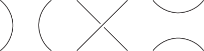
Consider now a triple of more general tangles $\mathcal{T}_{k}=(Y,T_{k})$, where $Y$ is a compact, oriented $3$-manifold (possibly) with boundary and each $(T_{k},\partial T_{k})\subset(Y,\partial Y)$ is a smoothly embedded compact $1$-dimensional submanifold, such that

• There is an embedded $\overline{B^{3}}$ in the interior of $Y$ in which $T_{k}$ coincides with $T^{\mathrm{el}}_{k}$; and

• For $k\in\mathchoice{\left\{\infty,0,1\right\}}{\{\infty,0,1\}}{\{\infty,0,1\}}{\{\infty,0,1\}}$, the tangles $T_{k}$ are identical outside $\overline{B^{3}}$.

Suppose each tangle complement $Y_{k}=Y\setminus\nu(T_{k})$ is equipped with a bordered–sutured structure $(\Gamma_{k},\mathcal{Z}_{1}\cup\mathcal{Z}_{2},\phi_{k})$, such that

• The sutures in $\Gamma_{k}$ do not intersect $\overline{B^{3}}$, and are identical for $k\in\mathchoice{\left\{\infty,0,1\right\}}{\{\infty,0,1\}}{\{\infty,0,1\}}{\{\infty,0,1\}}$;

• The intersection of $\partial Y_{k}$ and $\overline{B^{3}}$ belongs to the positive region $R_{+}(\Gamma)$; and

• The bordered boundary, i.e. the image of the parametrization $\phi_{k}\colon G(\mathcal{Z}_{1}\cup\mathcal{Z}_{2})\hookrightarrow\partial Y_{k}$, does not intersect $\overline{B^{3}}$, and the parametrization maps are identical for $k\in\mathchoice{\left\{\infty,0,1\right\}}{\{\infty,0,1\}}{\{\infty,0,1\}}{\{\infty,0,1\}}$.

Note that either of $\mathcal{Z}_{1}$ and $\mathcal{Z}_{2}$ may be empty or not connected. To each bordered–sutured manifold $\mathcal{Y}_{k}=(Y_{k},\Gamma_{k},\mathcal{Z}_{1}\cup\mathcal{Z}_{2},\phi_{k})$, then, Zarev [Zar11:BSFH] associates a type $\mathit{DA}$ bimodule

$$\itensor[^{\mathcal{A}(-\mathcal{Z}_{1})}]{\widehat{\operatorname{BSDA}}(\mathcal{Y}_{k})}{{}_{\mathcal{A}(\mathcal{Z}_{2})}}.$$

over $\mathcal{A}(-\mathcal{Z}_{1})$ and $\mathcal{A}(\mathcal{Z}_{2})$. A similar construction is used to obtain a bordered–sutured manifold $\mathcal{Y}_{\Gamma}(\mathcal{T})$ by Alishahi and Lipshitz [AliLip17:BFHCompressingDisks], who prove that $\widehat{\operatorname{BSD}}(\mathcal{Y}_{\Gamma}(\mathcal{T}))$ detects (partly) boundary parallel tangles. Our hypothesis differs from their construction in that we do not allow longitudinal sutures that intersect $\overline{B^{3}}$, but we do allow non–null-homologous $\mathcal{T}$ and place no restrictions on the sutures or the bordered boundaries outside $\overline{B^{3}}$.

Theorem 1.1.

Let $\mathcal{Y}_{k}$ be as described above. There exist type $\mathit{DA}$ homomorphisms $F_{k}\colon\widehat{\operatorname{BSDA}}(\mathcal{Y}_{k})\to\widehat{\operatorname{BSDA}}(\mathcal{Y}_{k+1})$ such that

$$\widehat{\operatorname{BSDA}}(\mathcal{Y}_{k})\simeq\operatorname{Cone}(F_{k+1}\colon\widehat{\operatorname{BSDA}}(\mathcal{Y}_{k+1})\to\widehat{\operatorname{BSDA}}(\mathcal{Y}_{k+2}))$$

as type $\mathit{DA}$ structures. Moreover, the homomorphisms $F_{k}$ and the homotopy equivalence above respect the relative gradings on the bimodules in a sense to be made precise in LABEL:sec:gradings; see LABEL:thm:gradings.

Because of the more complicated nature of the gradings, we generally defer their discussions to LABEL:sec:gradings.

The strategy to prove Theorem 1.1 is to consider bordered–sutured manifolds $\mathcal{B}_{k}$ corresponding to the complements of the elementary tangles $\mathcal{T}^{\mathrm{el}}_{k}$, first defining homomorphisms $f_{k}\colon\widehat{\operatorname{BSD}}(\mathcal{B}_{k})\to\widehat{\operatorname{BSD}}(\mathcal{B}_{k+1})$, and then using the pairing theorem [Zar11:BSFH, Theorem 8.5.1] to extend the result to our setting. In fact, it is evident from our strategy that the skein relation above holds for more general bordered–sutured manifolds $\mathcal{Y}_{k}$ and not just tangle complements; for example, one may derive from Theorem 1.1 a skein relation for (a generalization of) graph Floer homology, defined by Harvey and O’Donnol [HarODo17:HFG], and independently by Bao [Bao17:HFG], for certain kinds of spatial graphs. The statement of Theorem 1.1 is chosen to emphasize our interest in the application of bordered–sutured Floer theory to the study of knots, links, and tangles. See LABEL:thm:general for the more general statement.

Our strategy illustrates and harnesses the power of a bordered theory, which allows one to use cut-and-paste techniques to prove general results by working locally. For example, in a similar spirit, Lipshitz, Ozsváth, and Thurston [LipOzsThu14:BFHBranchedDoubleSSI, LipOzsThu16:BFHBranchedDoubleSSII] have used bordered Floer homology to compute explicitly the spectral sequence from Khovanov homology of a link to the Heegaard Floer homology of its branched double cover [OzsSza05:HFBranchedDoubleSS].

In particular, our strategy offers an advantage over the proofs in [Man07:HFKUnorientedSkein, Won17:GHUnorientedSkein, PetWon18:TFHSkein], as follows. In Manolescu’s original paper [Man07:HFKUnorientedSkein], the maps involved in the exact sequence are defined by counting holomorphic polygons in a high-dimensional manifold, which are of theoretical interest but not practically computable. In contrast, the maps in [Won17:GHUnorientedSkein] are combinatorially defined, which is a feature specifically exploited in the application to mutation invariance [Lam17:GHMutation]; the maps in [PetWon18:TFHSkein] are likewise combinatorial. However, while we believe the maps in [Won17:GHUnorientedSkein, PetWon18:TFHSkein] coincide with holomorphic polygon counts, it is not immediately obvious that they are so; moreover, the complexes involved there are fairly large. The present paper unites the two approaches: We will first define $f_{k}$ by counts of holomorphic triangles in LABEL:sec:skein_via_polygon, and then explicitly compute them combinatorially in LABEL:sec:skein_via_computation, taking advantage of the fact that $\widehat{\operatorname{BSD}}(\mathcal{B}_{k})$ have at most three generators with our choice of bordered–sutured Heegaard diagrams $\mathcal{H}_{k}$. The reader is encouraged to take a cursory look at LABEL:fig:comm_diag_f and LABEL:fig:comm_diag_phi, which contain the entire computation.

A special case of Theorem 1.1 is when $Y$ is a compact $3$-manifold without boundary, with $\mathcal{Z}_{1}=\mathcal{Z}_{2}=\varnothing$. In this case, each $T_{k}$ is an embedded $1$-dimensional submanifold without boundary, and is hence a link in $Y$; we thus denote it more conventionally by $L_{k}$. Let $\ell_{k}$ be the number of components of $L_{k}$, and set $m=\max\mathchoice{\left\{\ell_{\infty},\ell_{0},\ell_{1}\right\}}{\{\ell_{\infty},\ell_{0},\ell_{1}\}}{\{\ell_{\infty},\ell_{0},\ell_{1}\}}{\{\ell_{\infty},\ell_{0},\ell_{1}\}}$.

Corollary 1.2.

There exists an exact triangle

$$\dotsb\xrightarrow{(F_{1})_{*}}\widehat{\operatorname{HFK}}(Y,L_{\infty})\otimes V^{m-\ell_{\infty}}\xrightarrow{(F_{\infty})_{*}}\widehat{\operatorname{HFK}}(Y,L_{0})\otimes V^{m-\ell_{0}}\xrightarrow{(F_{0})_{*}}\widehat{\operatorname{HFK}}(Y,L_{1})\otimes V^{m-\ell_{1}}\xrightarrow{(F_{1})_{*}}\dotsb,$$

where $V$ is a vector space of dimension $2$. Moreover, the maps involved respect the relative gradings on the homology groups in a sense to be made precise in LABEL:sec:gradings; see LABEL:thm:gradings.

The reader familiar with gradings in sutured Floer homology may find it useful to examine LABEL:eg:iden_fibers_2 for an illustration of the graded version of Corollary 1.2.

The exact triangle in [Man07:HFKUnorientedSkein] is the special case $Y=S^{3}$. In [Man07:HFKUnorientedSkein], Manolescu constructs, from a given connected link projection of $L_{\infty}\subset S^{3}$ and a choice of edges in the projection, a special Heegaard diagram $\mathcal{H}^{\mathrm{Man}}_{\infty}$ for $L_{\infty}$, modifies $\mathcal{H}^{\mathrm{Man}}_{\infty}$ locally to obtain Heegaard diagrams $\mathcal{H}^{\mathrm{Man}}_{0}$ and $\mathcal{H}^{\mathrm{Man}}_{1}$ for $L_{0}$ and $L_{1}$, and uses these Heegaard diagrams to prove the skein exact triangle. Here, we have added a superscript to distinguish these Heegaard diagrams defined in [Man07:HFKUnorientedSkein] from those constructed in the present article; likewise, we denote by $F^{\mathrm{Man}}_{k}$ the maps involved in the skein exact triangle, which are denoted $f_{k}$ in [Man07:HFKUnorientedSkein].

Note that one might be able to prove Corollary 1.2 by directly generalizing Manolescu’s construction; however, that would require constructing Heegaard diagrams of a given form, for all $(Y,L_{\infty})$, which could be somewhat cumbersome before the advent of bordered–sutured Floer theory. (See, for contrast, the discussion after LABEL:thm:comm_spec.)

Theorem 1.3.

For $Y=S^{3}$, the exact triangle in Corollary 1.2 agrees with the exact triangle in [Man07:HFKUnorientedSkein]. See LABEL:thm:agree_2 for the precise statement.

In [ManOzs08:QALinks] (and in [Won17:GHUnorientedSkein, PetWon18:TFHSkein]), the exact triangles are equipped with an absolute $\delta$-grading in $\mathbb{Z}$. While we expect the grading in Corollary 1.2 to be related to this $\delta$-grading when applied to $Y=S^{3}$, we do not prove this in this paper. See, however, LABEL:rmk:gr_01.

Theorem 1.3 is inspired by [LipOzsThu16:BFHBranchedDoubleSSII], in which the theory of bordered polygon counts is developed to prove that the exact triangle, and in fact the spectral sequence, constructed in [LipOzsThu14:BFHBranchedDoubleSSI] using bordered Floer homology, agree with the original exact triangle and spectral sequence constructed directly using Heegaard Floer homology [OzsSza05:HFBranchedDoubleSS].

Organization

The rest of the paper is organized as follows. In Section 2, we fix some notation and provide a lemma in homological algebra that will be useful in later sections. Then, in Section 3, we describe the bordered boundary and the bordered–sutured manifolds $\mathcal{B}_{k}$, which correspond to the complements of the elementary tangles $T^{\mathrm{el}}_{k}$, and explicitly compute the algebra and modules associated to these objects. Stating and assuming the specialization of Theorem 1.1 to $\mathcal{B}_{k}$, we complete the general proof of Theorem 1.1 and Corollary 1.2. We provide two proofs of the specialization. We first give a theoretical proof by holomorphic polygon counts in LABEL:sec:skein_via_polygon, in the process adapting the technique of polygon counts from [LipOzsThu16:BFHBranchedDoubleSSII] to the bordered–sutured setting. Then, in LABEL:sec:skein_via_computation, we give a combinatorial proof, with explicit computations, and show that the two proofs are equivalent. We then compare our maps with Manolescu’s maps [Man07:HFKUnorientedSkein] and establish Theorem 1.3 in LABEL:sec:comparison. Finally, in LABEL:sec:gradings, we discuss the gradings in bordered–sutured Floer theory in some detail and prove a graded version of Theorem 1.1.

Acknowledgements

The authors would like to thank Robert Lipshitz for helpful discussions.

2. Algebraic preliminaries

We shall assume that the reader is familiar with the formal algebraic structures in the bordered Floer package [LipOzsThu18:BFH, LipOzsThu15:BFHBimodules] and the bordered–sutured Floer package [Zar11:BSFH]. (For the reader familiar with the former but not the latter, the algebraic structures involved are the same.) These include type $D$ and type $A$ modules, bimodules of various types, morphisms of modules and their boundaries and compositions, and the box tensor operation of modules. In general, we follow the notation in [Zar11:BSFH], which may differ from the notation in [LipOzsThu18:BFH]; see, however, LABEL:rmk:order.

In the following, we will always use the calligraphic typeface (e.g. $\mathcal{M}$ and $\mathcal{N}$) to denote an unspecified type $D$ or type $A$ module over some algebra $\mathcal{A}$, and reserve the regular italic typeface (e.g. $M$ and $N$) for the underlying $\mathbf{k}$-module. However, we will denote both the type $D$ bordered–sutured Floer module over the algebra $\mathcal{A}(\mathcal{Z})$, and the underlying $\mathbf{k}$-module, by $\widehat{\operatorname{BSD}}(\mathcal{Y})$. We will also distinguish between the identity type $D$ homomorphism $\mathbb{I}_{\mathcal{M}}$ of $\mathcal{M}$ and the identity $\mathbf{k}$-module isomorphism $\operatorname{id}_{M}$ of $M$.

Given a type $D$ morphism $f\colon\mathcal{M}\to\mathcal{N}$, let $\partial f$ denote its boundary in $\operatorname{Mor}^{\mathcal{A}}(\mathcal{M},\mathcal{N})$, given by

$$\partial f=(\mu\otimes\operatorname{id}_{N})\circ(\operatorname{id}_{A}\otimes\delta_{N})\circ f+(\mu\otimes\operatorname{id}_{N})\circ(\operatorname{id}_{A}\otimes f)\circ\delta_{M}+(d\otimes\operatorname{id}_{N})\circ f.$$

For convenience, we sometimes denote by $df$ the term $(d\otimes\operatorname{id}_{N})\circ f$.

The proof of Theorem 1.1 uses a lemma in homological algebra whose version for chain complexes first appeared in [OzsSza05:HFBranchedDoubleSS]. Let $\mathcal{A}=(A,d,\mu)$ be a differential graded algebra, and let $\mathcal{M}$ and $\mathcal{N}$ be type $D$ modules over $\mathcal{A}$.

Lemma 2.1.

Let $\mathcal{M}_{k}=\mathchoice{\left\{(M_{k},\delta_{M_{k}})\right\}}{\{(M_{k},\delta_{M_{k}})\}}{\{(M_{k},\delta_{M_{k}})\}}{\{(M_{k},\delta_{M_{k}})\}}_{k\in\mathchoice{\left\{\infty,0,1\right\}}{\{\infty,0,1\}}{\{\infty,0,1\}}{\{\infty,0,1\}}}$ be a collection of type $D$ modules over a unital differential graded algebra $\mathcal{A}=(A,d,\mu)$ over a base ring $\mathbf{k}$ of characteristic $2$, and let $f_{k}\colon\mathcal{M}_{k}\to\mathcal{M}_{k+1}$, $\varphi_{k}\colon\mathcal{M}_{k}\to\mathcal{M}_{k+2}$, and $\kappa_{k}\colon\mathcal{M}_{k}\to\mathcal{M}_{k}$ be morphisms satisfying the following conditions for each $k$:

1. The morphism $f_{k}\colon\mathcal{M}_{k}\to\mathcal{M}_{k+1}$ is a type $D$ homomorphism, i.e.

   $$\partial f_{k}=0;$$

2. The morphism $f_{k+1}\circ f_{k}$ is homotopic to zero via homotopy $\varphi_{k}$, i.e.

   $$f_{k+1}\circ f_{k}+\partial\varphi_{k}=0;$$

3. The morphism $f_{k+2}\circ\varphi_{k}+\varphi_{k+1}\circ f_{k}$ is homotopic to the identity $\mathbb{I}_{k}$ via homotopy $\kappa_{k}$, i.e.

   $$f_{k+2}\circ\varphi_{k}+\varphi_{k+1}\circ f_{k}+\partial\kappa_{k}=\mathbb{I}_{k}.$$

A graphical representation of the conditions above is given in Figure 2. Then for each $k$, the type $D$ modules $\mathcal{M}_{k}$ is homotopy equivalent to the mapping cone $\operatorname{Cone}(f_{k+1})$.

((1))

((2))

((3))

Figure 2. Graphical representations of the conditions in Lemma 2.1.

Proof.

This is a special case of [PetWon18:TFHSkein, Lemma 2.1], where $B=\mathbb{F}_{2}$ is the trivial algebra. ∎

3. The bordered–sutured Floer package of elementary tangle complements

In this section, we explicitly compute the differential graded algebra and type $D$ modules that we will be working with in the rest of the paper. For the sake of economy, we do not provide the definitions of the algebras and modules in bordered–sutured Floer theory, but direct the reader to [Zar11:BSFH].

3.1. The algebra associated to a 4-punctured sphere

Let $F$ be the $4$-punctured sphere, and let $\mathcal{F}$ be the sutured surface $(F,\Lambda)$, where $\Lambda$ consists of $2$ distinct points on each component of $\partial F$. In other words, each boundary circle of $F$ is divided into a positive and a negative arc.

In the context of tangles, $\mathcal{F}$ will be the bordered part of the boundary of a tangle complement, along which another bordered–sutured manifold can be glued. Thus, our first task is to parametrize $\mathcal{F}$ by an arc diagram $-\mathcal{Z}$. (The orientation reversal is appropriate for type $D$ structures.)

Let $\mathbf{Z}=\mathchoice{\left\{Z_{1},Z_{2},Z_{3},Z_{4}\right\}}{\{Z_{1},Z_{2},Z_{3},Z_{4}\}}{\{Z_{1},Z_{2},Z_{3},Z_{4}\}}{\{Z_{1},Z_{2},Z_{3},Z_{4}\}}$ be a collection of oriented arcs, and let $\mathbf{a}=\mathchoice{\left\{a_{1},\dotsc,a_{12}\right\}}{\{a_{1},\dotsc,a_{12}\}}{\{a_{1},\dotsc,a_{12}\}}{\{a_{1},\dotsc,a_{12}\}}$ be a collection of distinct points in $\mathbf{Z}$, such that

$$a_{1}\in Z_{1},\quad a_{2},a_{3},a_{4},a_{5}\in Z_{2},\quad a_{6},a_{7},a_{8},a_{9}\in Z_{3},\quad a_{10},a_{11},a_{12}\in Z_{4},$$

in this order, if we traverse the arcs $Z_{i}$ according to their orientations. Let $M\colon\mathbf{a}\to\mathchoice{\left\{1,\dotsc,6\right\}}{\{1,\dotsc,6\}}{\{1,\dotsc,6\}}{\{1,\dotsc,6\}}$ be the matching

$$M(a_{1}) =M(a_{3})=1, M(a_{2}) =M(a_{5})=2, M(a_{4}) =M(a_{7})=3,$$

$$M(a_{6}) =M(a_{9})=4, M(a_{8}) =M(a_{11})=5, M(a_{10}) =M(a_{12})=6.$$

If we define $\mathcal{Z}=(\mathbf{Z},\mathbf{a},M)$, then $-\mathcal{Z}$ parametrizes $\mathcal{F}(-\mathcal{Z})=\mathcal{F}$, as in Figure 3.

2pt $a_{1}$ [r] at 28 10 $a_{2}$ [r] at 28 35 $a_{3}$ [r] at 28 45 $a_{4}$ [r] at 28 55 $a_{5}$ [r] at 28 64 $a_{6}$ [r] at 28 85 $a_{7}$ [r] at 28 95 $a_{8}$ [r] at 28 104 $a_{9}$ [r] at 28 114 $a_{10}$ [r] at 28 137 $a_{11}$ [r] at 28 148 $a_{12}$ [r] at 28 159

$\rho_{1}$ [r] at 21 39 $\rho_{2}$ [r] at 21 50 $\rho_{3}$ [r] at 21 60 $\rho_{4}$ [r] at 21 90 $\rho_{5}$ [r] at 21 100 $\rho_{6}$ [r] at 21 109 $\rho_{7}$ [r] at 21 142 $\rho_{8}$ [r] at 21 153

$Z_{1}$ [r] at 1 10 $Z_{2}$ [r] at 1 50 $Z_{3}$ [r] at 1 100 $Z_{4}$ [r] at 1 148

$e_{1}$ [r] at 62 26 $e_{2}$ [r] at 62 50 $e_{3}$ [r] at 62 75 $e_{4}$ [r] at 62 100 $e_{5}$ [r] at 62 125 $e_{6}$ [r] at 62 148

$\cong$ [r] at 153 78 $Z_{1}$​​

Figure 3. Left: The arc diagram $\mathcal{Z}$. Center and right: The sutured surface $\mathcal{F}(-\mathcal{Z})=(F,\Lambda)$, where $F$ is a $4$-punctured sphere.