Error analysis of an accelerated interpolative decomposition for 3D Laplace problems

Abstract

In constructing the $\mathcal{H}^{2}$ representation of dense matrices defined by the Laplace kernel, the interpolative decomposition of certain off-diagonal submatrices that dominates the computation can be dramatically accelerated using the concept of a proxy surface. We refer to the computation of such interpolative decompositions as the proxy surface method. We present an error bound for the proxy surface method in the 3D case and thus provide theoretical guidance for the discretization of the proxy surface in the method.

Abstract

In constructing the $\mathcal{H}^{2}$ representation of dense matrices defined by the Laplace kernel, the interpolative decomposition of certain off-diagonal submatrices that dominates the computation can be dramatically accelerated using the concept of a proxy surface. We refer to the computation of such interpolative decompositions as the proxy surface method. We present an error bound for the proxy surface method in the 3D case and thus provide theoretical guidance for the discretization of the proxy surface in the method.

1 Introduction

$\mathcal{H}^{2}$ matrix techniques [1, 2, 3] can accelerate dense matrix-vector multiplications and also provide efficient direct solvers for many types of dense kernel matrices arising from the discretization of integral equations. However, these benefits are based on a rather expensive $\mathcal{H}^{2}$ matrix construction cost. Given a kernel function $K(x,y)$, the main bottleneck of $\mathcal{H}^{2}$ construction using interpolative decomposition (ID) [4, 5, 6] is the ID approximation of certain kernel submatrices of the form $K(X_{0},Y_{0})$ where point set $X_{0}$ lies in a bounded domain $\mathcal{X}$ and point set $Y_{0}$ lies in the far field of $\mathcal{X}$, denoted as $\mathcal{Y}$, with $Y_{0}$ usually much larger than $X_{0}$. A 2D example of $X_{0}$ and $Y_{0}$ is shown in Figure 1.

Figure 1: Illustration of the proxy surface method. The matrix to be directly compressed is $K(X_{0},Y_{p})$, rather than $K(X_{0},Y_{0})$, with a fixed number of columns $|Y_{p}|$, regardless of how many points $Y_{0}$ there are in $\mathcal{Y}$.

An algebraic approach to obtain these IDs usually leads to a prohibitive quadratic $\mathcal{H}^{2}$ construction cost. For the Laplace kernel, Martinsson and Rohklin [7] efficiently obtained an ID of $K(X_{0},Y_{0})$ by using the concept of a proxy surface and this concept is also used in recursive skeletonization by Ho and Greengard [5]. The key idea, as illustrated in Figure 1, is to convert the problem into the ID approximation of a kernel matrix $K(X_{0},Y_{p})$, where point set $Y_{p}$ is selected to discretize the interior boundary of $\mathcal{Y}$, with $Y_{p}$ much smaller than $Y_{0}$ in practice. The interior boundary, denoted as $\Gamma$, is called a proxy surface in [5] and thus we refer to the method as the proxy surface method. With this method, the $\mathcal{H}^{2}$ construction cost can be reduced to linear complexity. It is worth noting that kernel independent FMM [8] and the proxy point method [9] are also based on similar ideas.

The error analysis of the proxy surface method, however, is only briefly discussed in [7] without much detail and the selection of $Y_{p}$ to discretize the proxy surface is heuristic in previous applications [7, 5, 10, 11]. In this paper, we provide a detailed error analysis of the proxy surface method for the 3D Laplace kernel. The error analysis shows that, under certain conditions, it is sufficient to discretize proxy surfaces of different sizes using a constant number of points while maintaining a fixed accuracy in the method.

2 Background

Given a matrix $A\in\mathbb{R}^{n\times m}$, a rank-$k$ interpolative decomposition (ID) [12, 13] of $A$ is of the form $UA_{J}$ where $A_{J}\in\mathbb{R}^{k\times m}$ is a row subset of $A$ and $U\in\mathbb{R}^{n\times k}$ has bounded entries. We call $A_{J}$ and $U$ the skeleton and projection matrices, respectively. The ID is said to have precision $\varepsilon$ if the norm of each row of the error matrix $A-UA_{J}$ is bounded by $\varepsilon$. Using an algebraic approach, the ID can be calculated based on the strong rank-revealing QR (sRRQR) [13] of $A^{T}$ with entries of the obtained $U$ bounded by a pre-specified parameter $C\geqslant 1$.

Take the domain pair $\mathcal{X}\times\mathcal{Y}$ and the interior boundary $\Gamma$ of $\mathcal{Y}$ shown in Figure 1 as an example. For the Laplace kernel $K(x,y)$ and any point sets $X_{0}\subset\mathcal{X}$ and $Y_{0}\subset\mathcal{Y}$, we now explain the proxy surface method for the ID approximation of $K(X_{0},Y_{0})$, based on the discussion from [7].

By Green’s Theorem, the potential at any $x\in\mathcal{X}$ generated by source point set $Y_{0}$ with charges $F=(f_{i})_{y_{i}\in Y_{0}}$ can also be generated by an equivalent charge distribution on the proxy surface $\Gamma$ that encloses $\mathcal{X}$. Select a point set $Y_{p}$ uniformly distributed on $\Gamma$ to discretize the equivalent charge distribution with point charges $\tilde{F}=(\tilde{f_{i}})_{y_{i}\in Y_{p}}$ at $Y_{p}$. It is shown in [7] that

$$\tilde{F}\approx W_{Y_{0},Y_{p}}F,$$

where $W_{Y_{0},Y_{p}}$ is a discrete approximation of the linear operator that maps charges $F$ at $Y_{0}$ to an equivalent charge distribution on $\Gamma$ with $\|W_{Y_{0},Y_{p}}\|_{2}$ bounded as a consequence of Green’s Theorem. Matching the potentials induced by $F$ and by $\tilde{F}$ at any $x\in\mathcal{X}$ gives $K(x,Y_{0})F\approx K(x,Y_{p})W_{Y_{0},Y_{p}}F$ and thus it holds that

$$K(x,Y_{0})\approx K(x,Y_{p})W_{Y_{0},Y_{p}},\quad\forall x\in\mathcal{X},$$ (1)

where $K(x,Y_{0})=(K(x,y_{i}))_{y_{i}\in Y_{0}}$ and $K(x,Y_{p})=(K(x,y_{i}))_{y_{i}\in Y_{p}}$ are both row vectors. Substituting $X_{0}\subset\mathcal{X}$ into Equation 1, the target matrix $K(X_{0},Y_{0})$ can be approximated as $K(X_{0},Y_{p})W_{Y_{0},Y_{p}}$. Find an ID of $K(X_{0},Y_{p})$ using sRRQR as

$$K(X_{0},Y_{p})\approx UK(X_{\text{rep}},Y_{p}),$$ (2)

where $X_{\text{rep}}\subset X_{0}$ denotes the “representative” point subset associated with the selected row subset in the skeleton matrix of the ID with $U$ being the projection matrix of the ID. The proxy surface method then defines the ID of $K(X_{0},Y_{0})$ as

$$K(X_{0},Y_{0})\approx UK(X_{\text{rep}},Y_{0}).$$ (3)

The error of the above approximation can be bounded as

$$\|K(X_{0},Y_{0})-UK(X_{\text{rep}},Y_{0})\|_{F} \approx\|\left(K(X_{0},Y_{p})-UK(X_{\text{rep}},Y_{p})\right)W_{Y_{0},Y_{p}}\|_{F}$$

$$\leqslant\|K(X_{0},Y_{p})-UK(X_{\text{rep}},Y_{p})\|_{F}\|W_{Y_{0},Y_{p}}\|_{2},$$

and thus the error is controlled by the error of the ID in Equation 2.

The number of points in $Y_{p}$ used to discretize $\Gamma$ is usually chosen heuristically. Ref. [7, 10] suggest using $|Y_{p}|\sim O(|X_{0}|)$ and [5] claims correctly but without an explanation that for the Laplace kernel, proxy surfaces of different sizes can be discretized using a constant number of points and this constant only depends on the compression precision.

In this paper, to theoretically justify the proxy surface method, we address the following two problems: (a) the quantitative relationship between the errors of the two IDs in Equation 2 and Equation 3 and (b) how to choose the number of points in $Y_{p}$ to guarantee the accuracy of the proposed ID in Equation 3.

3 Main result

We focus on the proxy surface method for the 3D Laplace kernel $K(x,y)=1/|x-y|$. Denote the open ball of radius $r$ centered at the origin as $B(0,r)$. For conciseness of the error analysis, we consider $\mathcal{X}=B(0,r_{1})$, $\mathcal{Y}=\mathbb{R}^{3}\backslash B(0,r_{2})$, and $\Gamma=\partial B(0,r_{2})$ with $r_{2}>r_{1}$, as illustrated in Figure 2. Assume a point set $Y_{p}$ has been selected to discretize $\Gamma$ and the target kernel matrix $K(X_{0},Y_{0})$ is associated with point sets $X_{0}\subset\mathcal{X}$ and $Y_{0}\subset\mathcal{Y}$.

Figure 2: 2D illustration of the 3D domain pair $\mathcal{X}\times\mathcal{Y}$ and the proxy surface $\Gamma$.

In the proxy surface method, the proposed ID in Equation 3 can be viewed row-by-row as

$$K(x_{i},Y_{0})\approx u_{i}^{T}K(X_{\text{rep}},Y_{0}),\quad x_{i}\in X_{0},$$

where $u_{i}^{T}$ denotes the $i$th row of $U$. Since the above approximation can be applied to any point set $Y_{0}$ in $\mathcal{Y}$, its error is intrinsically based on the function approximation

$$K(x_{i},y)\approx u_{i}^{T}K(X_{\text{rep}},y),\quad x_{i}\in X_{0},\ y\in\mathcal{Y}.$$

Denote the error of this function approximation by the scalar function

$$e_{i}(y)=K(x_{i},y)-u_{i}^{T}K(X_{\text{rep}},y),\quad x_{i}\in X_{0},\ y\in\mathcal{Y}.$$ (4)

In other words, $e_{i}(y)$ is the error in the approximation of the interaction between $x_{i}$ and some $y\in\mathcal{Y}$. Using this notation, the error of the $i$th row of the approximations Equation 2 and Equation 3 can be denoted as $e_{i}(Y_{0})$ and $e_{i}(Y_{p})$, respectively, which are row vectors. In the following discussion, we assume that the ID Equation 2 of $K(X_{0},Y_{p})$ has precision $\varepsilon\sqrt{|Y_{p}|}$ and thus $\|e_{i}(Y_{p})\|_{2}\leqslant\varepsilon\sqrt{|Y_{p}|}$.

For $Y_{0}\subset\mathcal{Y}$ with an arbitrary point distribution, the best upper bound for $e_{i}(Y_{0})$ is

$$\|e_{i}(Y_{0})\|_{2}\leqslant\sqrt{|Y_{0}|}\max_{y\in\mathcal{Y}}|e_{i}(y)|.$$ (5)

Our error analysis of the proxy surface method seeks an upper bound for $|e_{i}(y)|$ in the whole domain $\mathcal{Y}$ under the condition that $\|e_{i}(Y_{p})\|_{2}\leqslant\varepsilon\sqrt{|Y_{p}|}$. In fact, we can prove the following proposition.

Proposition 1.

If point set $Y_{p}\subset\Gamma$ satisfies the condition that numerical quadrature with the points in $Y_{p}$ and equal weights $\frac{4\pi r_{2}^{2}}{|Y_{p}|}$ is exact for polynomials on $\Gamma$ of degree up to $2c$ where $c$ is an integer constant, then $e_{i}(y)$ for any $x_{i}\in X_{0}$ can be bounded as

$$|e_{i}(y)|\leqslant(c+1)\frac{\|e_{i}(Y_{p})\|_{2}}{\sqrt{|Y_{p}|}}+(c+2)\frac{(1+|X_{\textnormal{rep}}|\|u_{i}\|_{\infty})}{r_{2}-r_{1}}\left(\frac{r_{1}}{r_{2}}\right)^{c+1}\!\!,\ y\in\mathcal{Y}.$$ (6)

Proof.

For any $x\in\mathcal{X}$, $K(x,y)$ as a function of $y$ is harmonic in $\mathcal{Y}$. Since $e_{i}(y)$ is a linear combination of $K(x_{i},y)$ and $\{K(x_{j},y):x_{j}\in X_{\text{rep}}\}$, it is also harmonic in $\mathcal{Y}$. By the maximum principle of harmonic functions, $e_{i}(y)$ satisfies

$$\max_{y\in\mathcal{Y}}|e_{i}(y)|=\max_{y\in\Gamma}|e_{i}(y)|.$$ (7)

Thus, it suffices to prove the upper bound Equation 6 for $y\in\Gamma$.

The multipole expansion of $K(x,y)$ with $(x,y)\in\mathcal{X}\times\Gamma$ is written as

$$K(x,y)=\sum_{l=0}^{\infty}\sum_{m=-l}^{l}M_{l}^{m}(x)\frac{1}{r_{2}^{l+1}}Y_{l}^{m}(\alpha,\beta),$$ (8)

where $(r_{2},\alpha,\beta)$ denotes the polar coordinates of $y$ on $\Gamma$, $\{Y_{l}^{m}(\alpha,\beta)\}$ is the set of spherical harmonics and $\left\{M_{l}^{m}(x)\right\}$ is a set of known analytic functions of $x$. Truncating the above infinite sum at index $c$, the remainder can be bounded as

$$\left|K(x,y)-\sum_{l=0}^{c}\sum_{m=-l}^{l}M_{l}^{m}(x)\frac{1}{r_{2}^{l+1}}Y_{l}^{m}(\alpha,\beta)\right|\leqslant\frac{1}{r_{2}-r_{1}}\left(\frac{r_{1}}{r_{2}}\right)^{c+1}.$$

Using the above multipole expansion, $e_{i}(y)$ on $\Gamma$ can be written as

$$e_{i}(y) =\sum_{l=0}^{\infty}\sum_{m=-l}^{l}\left(M_{l}^{m}(x_{i})-u_{i}^{T}M_{l}^{m}(X_{\text{rep}})\right)\frac{1}{r_{2}^{l+1}}Y_{l}^{m}(\alpha,\beta)$$

$$=\sum_{l=0}^{c}\sum_{m=-l}^{l}E_{l}^{m}Y_{l}^{m}(\alpha,\beta)+R_{c}(y),$$ (9)

where $E_{l}^{m}$ denotes the coefficient collected for $Y_{l}^{m}(\alpha,\beta)$ and the remainder $R_{c}(y)$ can be bounded as

$$|R_{c}(y)|\leqslant\frac{(1+|X_{\text{rep}}|\|u_{i}\|_{\infty})}{r_{2}-r_{1}}\left(\frac{r_{1}}{r_{2}}\right)^{c+1},$$

using the triangle inequality. Since $\{Y_{l}^{m}(\alpha,\beta)\}$ is an orthonormal function set on the unit sphere $\mathbb{S}^{2}$, the coefficients $E_{l}^{m}$ can be analytically calculated as

$$E_{l}^{m}=\int_{\mathbb{S}^{2}}e_{i}(r_{2}y)Y_{l}^{m}(y)\mathrm{d}y=\dfrac{1}{r_{2}^{2}}\int_{\Gamma}e_{i}(y)Y_{l}^{m}(y)\mathrm{d}y,$$

where $Y_{l}^{m}(y)$ is defined as $Y_{l}^{m}(\alpha,\beta)$ for any $y=(|y|,\alpha,\beta)$.

Since numerical quadrature with the points in $Y_{p}$ and equal weights $\frac{4\pi r_{2}^{2}}{|Y_{p}|}$ is exact for polynomials on $\Gamma$ of degree up to $2c$, $E_{l}^{m}$ with $l\leqslant c$ can be further represented as

$$E_{l}^{m}= \frac{1}{r_{2}^{2}}\int_{\Gamma}(e_{i}(y)-R_{c}(y))Y_{l}^{m}(y)\mathrm{d}y$$

$$= \frac{4\pi}{|Y_{p}|}\sum_{y_{j}\in Y_{p}}(e_{i}(y_{j})-R_{c}(y_{j}))Y_{l}^{m}(y_{j})$$

$$= \frac{4\pi}{|Y_{p}|}\left(e_{i}(Y_{p})-R_{c}(Y_{p})\right)^{T}Y_{l}^{m}(Y_{p}).$$ (10)

Substituting this $E_{l}^{m}$ into Equation 9, $e_{i}(y)$ on $\Gamma$ can be written as,

$$e_{i}(y)= \frac{4\pi}{|Y_{p}|}\left(e_{i}(Y_{p})\!-R_{c}(Y_{p})\right)^{T}\!\left(Y_{0}^{0}(Y_{p})\ Y_{1}^{-1}(Y_{p})\ \ldots\ Y_{c}^{c}(Y_{p})\right)\!\left(\begin{array}[]{c}Y_{0}^{0}(y)\\ Y_{1}^{-1}(y)\\ \vdots\\ Y_{c}^{c}(y)\end{array}\right)\!+R_{c}(y)$$ (15)

$$= \frac{4\pi}{|Y_{p}|}\left(e_{i}(Y_{p})-R_{c}(Y_{p})\right)^{T}M\Phi(y)+R_{c}(y),$$ (16)

where $M$ denotes the middle matrix and $\Phi(y)$ denotes the last vector function of $y$ in the first equation. Note that any two distinct columns of $M$, say $Y_{l_{1}}^{m_{1}}(Y_{p})$ and $Y_{l_{2}}^{m_{2}}(Y_{p})$, are orthogonal with

$$Y_{l_{1}}^{m_{1}}(Y_{p})^{T}Y_{l_{2}}^{m_{2}}(Y_{p})=\frac{|Y_{p}|}{4\pi}\int_{\mathbb{S}^{2}}Y_{l_{1}}^{m_{1}}(y)Y_{l_{2}}^{m_{2}}(y)\mathrm{d}y=\frac{|Y_{p}|}{4\pi}\delta_{l_{1}=l_{2},m_{1}=m_{2}},$$

and thus the scaled matrix $\sqrt{\frac{4\pi}{|Y_{p}|}}M$ has orthonormal columns. Therefore, it holds that

$$\sqrt{\frac{4\pi}{|Y_{p}|}}\left\|M\Phi(y)\right\|_{2}=\|\Phi(y)\|_{2}.$$

Meanwhile, by the property of spherical harmonics, the 2-norm of the vector function $\Phi(y)$ at any $y\in\Gamma$ is

$$\|\Phi(y)\|_{2}=\sqrt{\sum_{l=0}^{c}\sum_{m=-l}^{l}|Y_{l}^{m}(y)|^{2}}=\sqrt{\sum_{l=0}^{c}\frac{2l+1}{4\pi}}=\frac{c+1}{\sqrt{4\pi}}.$$

Based on Equation 16, we can obtain the final upper bound by using the Cauchy-Schwarz and triangle inequalities as follows,

$$|e_{i}(y)| \leqslant\left|\frac{4\pi}{|Y_{p}|}e_{i}(Y_{p})^{T}M\Phi(y)\right|+\left|\frac{4\pi}{|Y_{p}|}R_{c}(Y_{p})^{T}M\Phi(y)\right|+|R_{c}(y)|$$

$$\leqslant\frac{4\pi}{|Y_{p}|}\|e_{i}(Y_{p})\|_{2}\|M\Phi(y)\|_{2}+\frac{4\pi}{|Y_{p}|}\|R_{c}(Y_{p})\|_{2}\|M\Phi(y)\|_{2}+|R_{c}(y)|$$

$$\leqslant(c+1)\frac{\|e_{i}(Y_{p})\|_{2}}{\sqrt{|Y_{p}|}}+(c+1)\frac{\|R_{c}(Y_{p})\|_{2}}{\sqrt{|Y_{p}|}}+|R_{c}(y)|$$

$$\leqslant(c+1)\frac{\|e_{i}(Y_{p})\|_{2}}{\sqrt{|Y_{p}|}}+(c+2)\frac{(1+|X_{\text{rep}}|\|u_{i}\|_{\infty})}{r_{2}-r_{1}}\left(\frac{r_{1}}{r_{2}}\right)^{c+1}.$$ (17)

∎

Combining Proposition 1 and inequality Equation 5, the error bound of the proxy surface method for the ID approximation of $K(X_{0},Y_{0})$ is described as follows.

Theorem 1 (Error bound for the proxy surface method).

If point set $Y_{p}$ satisfies the condition in Proposition 1 and the ID Equation 2 of $K(X_{0},Y_{p})$ has precision $\varepsilon\sqrt{|Y_{p}|}$, i.e., $\|e_{i}(Y_{p})\|_{2}\leqslant\varepsilon\sqrt{|Y_{p}|}$ for each $x_{i}\in X_{0}$, the ID Equation 3 of $K(X_{0},Y_{0})$ in the proxy surface method has error $e_{i}(Y_{0})$ at the $i$th row bounded as

$$\dfrac{\|e_{i}(Y_{0})\|_{2}}{\sqrt{|Y_{0}|}} \leqslant(c+1)\dfrac{\|e_{i}(Y_{p})\|_{2}}{\sqrt{|Y_{p}|}}+(c+2)\frac{(1+|X_{\textnormal{rep}}|\|u_{i}\|_{\infty})}{r_{2}-r_{1}}\left(\frac{r_{1}}{r_{2}}\right)^{c+1}$$ (18)

$$\leqslant(c+1)\varepsilon+(c+2)\frac{(1+|X_{\textnormal{rep}}|\|u_{i}\|_{\infty})}{r_{2}-r_{1}}\left(\frac{r_{1}}{r_{2}}\right)^{c+1}.$$ (19)

When there are not enough points in $Y_{p}$, i.e., $c$ is small, the error is dominated by the second term of the upper bound in Equation 19 which comes from the truncation error $R_{c}(y)$ in Equation 9. A simple interpretation is that controlling the values of $e_{i}(y)$ for $y\in Y_{p}$ through the ID approximation of $K(X_{0},Y_{p})$ is not sufficient to completely control $e_{i}(y)$ over the whole surface $\Gamma$.

4 Selection of $Y_{p}$

Using the quadrature point sets provided in [14], only $2c^{2}+2c+O(1)$ points are needed in $Y_{p}$ to make the associated numerical quadrature exact for polynomials on $\Gamma$ of degree up to $2c$. Thus, the key for the selection of $Y_{p}$ is to decide the smallest $c$ for a given error threshold to balance the precision and efficiency of the proxy surface method.

Since the error bound Equation 19 contains $|X_{\text{rep}}|$ and $\|u_{i}\|_{\infty}$ that depend on the ID of $K(X_{0},Y_{p})$, we need some a priori bounds of these two quantities for the selection of $Y_{p}$. When using sRRQR to find the ID of $K(X_{0},Y_{p})$, entries of $U$ can be bounded by a pre-specified parameter $C_{\text{qr}}\geqslant 1$ and thus $\|u_{i}\|_{\infty}\leqslant C_{\text{qr}}$ for any $x_{i}\in X_{0}$. $|X_{\text{rep}}|$ is a rank estimate of $K(X_{0},Y_{p})$ and thus satisfies $|X_{\text{rep}}|\leqslant\min(|X_{0}|,|Y_{p}|)$. Plugging these values into Equation 19, we obtain an a priori error bound as

$$\dfrac{\|e_{i}(Y_{0})\|_{2}}{\sqrt{|Y_{0}|}}\leqslant(c+1)\varepsilon+(c+2)\frac{C_{\text{qr}}\min\left(|X_{0}|,|Y_{p}|\right)+1}{r_{2}-r_{1}}\left(\frac{r_{1}}{r_{2}}\right)^{c+1}.$$

Heuristically, we choose the integer constant $c$ by making the second term above of scale $(c+1)\varepsilon$, i.e.,

$$\frac{C_{\text{qr}}\min\left(|X_{0}|,2c^{2}+2c+O(1)\right)+1}{r_{2}-r_{1}}\left(\frac{r_{1}}{r_{2}}\right)^{c+1}\approx\varepsilon.$$ (20)

$Y_{p}$ can then be directly obtained from the dataset of [14] with the selected $c$. The row approximation error of the proxy surface method is then bounded as

$$\|e_{i}(Y_{0})\|_{2}\leqslant(2c+3)\varepsilon\sqrt{|Y_{0}|}.$$ (21)

It is worth noting that the condition for $Y_{p}$ in Proposition 1 is mainly for a rigorous analysis and also that the obtained upper bounds Equation 19 and Equation 21 may not be tight. Thus, the above selection of $Y_{p}$ is conservative and may be unnecessarily large. However, the key idea conveyed by Theorem 1 and the above selection of $Y_{p}$ is that as long as $\Gamma$ and $\mathcal{X}$ are well-separated, e.g., $r_{2}-r_{1}\geqslant 1$, and the ratio of their radii is fixed, $Y_{p}$ with a constant number of points is sufficient to maintain the accuracy of the proxy surface method. Also, this theorem rigorously justifies the claim in [5] about using a constant number of points to discretize different proxy surfaces in recursive skeletonization.

5 Numerical experiments

We consider the 3D Laplace kernel $K(x,y)=1/|x-y|$. The error threshold for the ID approximation of $K(X_{0},Y_{p})$ is set as $\varepsilon\sqrt{|Y_{p}|}$ so that $\|e_{i}(Y_{p})\|_{2}\leqslant\varepsilon\sqrt{|Y_{p}|}$ for each $x_{i}\in X_{0}$ with $\varepsilon$ specified later. The entry-bound parameter $C_{\text{qr}}$ for sRRQR in the ID approximation of $K(X_{0},Y_{p})$ is set to $2$.

(a)

(b)

Figure 3: Values of $\max_{y\in\mathcal{Y}}|e_{i}(y)|$ and its upper bound given in Equation 6 for each $x_{i}\in X_{0}\backslash X_{\text{rep}}$ with (a) values of the two quantities and (b) ratio of the upper bound to $\max_{y\in\mathcal{Y}}|e_{i}(y)|$. Indices for $x_{i}\in X_{0}\backslash X_{\text{rep}}$ are sorted so that the upper bounds are in ascending order.

5.1 Error bound for $e_{i}(y)$ in Proposition 1

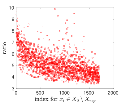
Consider domain pair $\mathcal{X}\times\mathcal{Y}=B(0,1)\times(\mathbb{R}^{3}\backslash B(0,2))$ and error threshold $\varepsilon=10^{-6}$. The corresponding constant $c$ estimated by Equation 20 is 30 and $Y_{p}$ selected from [14] has 1862 points. We randomly and uniformly select 2000 points in $\mathcal{X}$ for $X_{0}$. The ID of $K(X_{0},Y_{p})$ obtains $X_{\text{rep}}$ with 298 points and also defines $e_{i}(y)$ for each $x_{i}\in X_{0}$.

To check the error bound Equation 6 in Proposition 1, we plot $\max_{y\in\mathcal{Y}}|e_{i}(y)|$ and its bound in Figure 3 for each $x_{i}\in X_{0}\backslash X_{\text{rep}}$  where, according to Equation 7, $\max_{y\in\mathcal{Y}}|e_{i}(y)|$ is estimated by densely sampling $|e_{i}(y)|$ over $\Gamma$. As can be observed, the upper bound in Proposition 1 is usually within an order of magnitude of $\max_{y\in\mathcal{Y}}|e_{i}(y)|$ for each $e_{i}(y)$. However, the ratio of these two quantities being always larger than 3 indicates that an even sharper upper bound may exist.

In a further numerical test, we vary the constant $c$ and thus the corresponding $Y_{p}$ selected from [14]. For each set of $e_{i}(y)$ obtained from different $Y_{p}$, in Figure 4, we plot $\max_{x_{i}\in X_{0},y\in\mathcal{Y}}|e_{i}(y)|$ and its upper bound derived from Proposition 1, i.e.,

$$\max_{x_{i}\in X_{0},y\in\mathcal{Y}}|e_{i}(y)|\leqslant(c+1)\varepsilon+(c+2)\dfrac{1+\max_{i}\|u_{i}\|_{\infty}|X_{\text{rep}}|}{r_{2}-r_{1}}\left(\dfrac{r_{1}}{r_{2}}\right)^{c+1}.$$ (22)

Figure 4: Values of $\max_{x_{i}\in X_{0},y\in\mathcal{Y}}|e_{i}(y)|$ and its upper bound Equation 22 for different constants $c$ and corresponding different point sets $Y_{p}$ selected from [14]. The error threshold $\varepsilon\sqrt{|Y_{p}|}$ with fixed $\varepsilon=10^{-6}$ is used in the ID approximation of $K(X_{0},Y_{p})$ for different $Y_{p}$.

From the numerical results, the upper bound Equation 22 is quite tight and it also catches the knee at $|Y_{p}|\approx 500$ where $\max_{x_{i}\in X_{0},y\in\mathcal{Y}}|e_{i}(y)|$ stops decreasing. Note that $\max_{x_{i}\in X_{0},y\in\mathcal{Y}}|e_{i}(y)|$ not further decreasing with larger $|Y_{p}|$ is due to the error threshold $\varepsilon\sqrt{|Y_{p}|}$ used in the ID approximation of $K(X_{0},Y_{p})$. The knee also shows that approximately 500 points for $Y_{p}$ should be enough to obtain the lowest error for the proxy surface method in this problem setting. However, the method of choosing $Y_{p}$ introduced in Section 4 gives $c=30$ and $|Y_{p}|=1862$. The main cause of this overestimation of $|Y_{p}|$, by comparing Equation 22 and Equation 20, turns out to be the looseness of $|X_{\text{rep}}|\leqslant\min(|X_{0}|,|Y_{p}|)$ utilized in Equation 20.

5.2 Error bound for $\|e_{i}(Y_{0})\|_{2}$ in Theorem 1

The bound for $\|e_{i}(Y_{0})\|_{2}$ in Theorem 1 simply combines the bound for $\max_{y\in\mathcal{Y}}|e_{i}(y)|$ in Proposition 1, which has been shown in the previous test to be quite tight, and the inequality Equation 5, i.e., $\|e_{i}(Y_{0})\|_{2}\leqslant\sqrt{|Y_{0}|}\max_{y\in\mathcal{Y}}|e_{i}(y)|$. Note that equality of Equation 5 can hold when $|e_{i}(y)|$ reaches its maximum at all the points in $Y_{0}$. However, for $Y_{0}$ with an arbitrary point distribution, this inequality turns out to be quite loose as illustrated below.

We use the same $\mathcal{X}\times\mathcal{Y}$, $\varepsilon$ and $X_{0}\subset\mathcal{X}$ as in the previous test and consider the point set $Y_{p}$ associated with $c=30$. We randomly and uniformly select 20000 points for $Y_{0}$ in two subdomains of $\mathcal{Y}$, $B(0,4)\backslash B(0,2)$ and $B(0,8)\backslash B(0,2)$. With the proxy surface method, the obtained average entry-wise error $\|e_{i}(Y_{0})\|_{2}/\sqrt{|Y_{0}|}$ and the maximum entry error $\max_{y\in Y_{0}}|e_{i}(y)|$ for each $x_{i}\in X_{0}\backslash X_{\text{rep}}$ are plotted in Figure 5 along with their shared upper bound Equation 18 given in Theorem 1.

(a) $Y_{0}\subset B(0,4)\backslash B(0,2)$

(b) $Y_{0}\subset B(0,8)\backslash B(0,2)$

Figure 5: Values of $\|e_{i}(Y_{0})\|_{2}/\sqrt{|Y_{0}|}$, $\max_{y\in Y_{0}}|e_{i}(y)|$ and their shared upper bound Equation 18 given in Theorem 1 with different point distributions in $Y_{0}$. Indices for $x_{i}\in X_{0}\backslash X_{\text{rep}}$ are sorted so that the upper bounds are in ascending order.

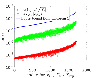
For both choices of the subdomain of $\mathcal{Y}$ (and $Y_{0}$), $\|e_{i}(Y_{0})\|_{2}/\sqrt{|Y_{0}|}$ is more than one order of magnitude smaller than $\max_{y\in Y_{0}}|e_{i}(y)|$. Thus, the inequality Equation 5 is quite loose in these cases.

5.3 Selection of $Y_{p}$

From Section 4, the selection of $Y_{p}$ mainly depends on the domain pair $\mathcal{X}\times\mathcal{Y}$ and the ID error threshold $\varepsilon\sqrt{|Y_{p}|}$. Varying these parameters, Table 1 lists the number of points in the selected $Y_{p}$. Although our selection scheme is quite conservative as shown in Figure 4, the results in Table 1 clearly show how the selection of $Y_{p}$ is affected by these parameters.

Table 1: Estimated constant $c$ and number of points in selected $Y_{p}$ under different settings of the radii $r_{1}$ and $r_{2}$ for the domain pair $\mathcal{X}\times\mathcal{Y}=B(0,r_{1})\times\left(\mathbb{R}^{3}\backslash B(0,r_{2})\right)$ and $\varepsilon$ in the ID error threshold $\varepsilon\sqrt{|Y_{p}|}$.

	$r_{1}$	$r_{2}$	$r_{1}/r_{2}$	$\varepsilon$	$c$	$|Y_{p}|$
reference test	1	2	0.5	$10^{-6}$	30	1862
different $\varepsilon$	1	2	0.5	$10^{-4}$	23	1106
	1	2	0.5	$10^{-8}$	38	2965
different $\dfrac{r_{1}}{r_{2}}$	1	4	0.25	$10^{-6}$	12	314
	1	6	0.16	$10^{-6}$	9	181
different $r_{2}-r_{1}$	10	20	0.5	$10^{-6}$	27	1514
	100	200	0.5	$10^{-6}$	23	1106

6 Conclusion

The error analysis in this paper rigorously confirms the accuracy of the proxy surface method by showing the quantitative relationship Equation 18 between the error of the ID of $K(X_{0},Y_{0})$ and the error of the ID of $K(X_{0},Y_{p})$. Also, the analysis justifies the use of a constant number of points to discretize proxy surfaces of different sizes in the hierarchical matrix construction of 3D Laplace kernel matrices, when the ratio $r_{1}/r_{2}$ is constant. The same error analysis technique can also be applied to the proxy surface method for more general matrices with entries defined by the interactions between two compact charge distributions, e.g., the matrix in the Galerkin method for integral equations and the electron repulsion integral tensors with Gaussian-type basis functions.

References

- [1] S. Chandrasekaran, M. Gu, T. Pals, A Fast ULV Decomposition Solver for Hierarchically Semiseparable Representations, SIAM Journal on Matrix Analysis and Applications 28 (3) (2006) 603–622.
- [2] W. Hackbusch, S. Börm, Data-sparse Approximation by Adaptive -Matrices, Computing 69 (1) (2002) 1–35.
- [3] W. Hackbusch, B. Khoromskij, S. A. Sauter, On -Matrices, Lectures on Applied Mathematics (2000) 9–29.
- [4] D. Cai, E. Chow, Y. Saad, Y. Xi, SMASH: Structured matrix approximation by separation and hierarchy, Numerical Linear Algebra with Applications, to appear (2018).
- [5] K. Ho, L. Greengard, A Fast Direct Solver for Structured Linear Systems by Recursive Skeletonization, SIAM Journal on Scientific Computing 34 (5) (2012) A2507–A2532.
- [6] P. G. Martinsson, A fast randomized algorithm for computing a hierarchically semiseparable representation of a matrix, SIAM Journal on Matrix Analysis and Applications 32 (4) (2011) 1251–1274.
- [7] P. G. Martinsson, V. Rokhlin, A fast direct solver for boundary integral equations in two dimensions, Journal of Computational Physics 205 (1) (2005) 1–23.
- [8] L. Ying, G. Biros, D. Zorin, A kernel-independent adaptive fast multipole algorithm in two and three dimensions, Journal of Computational Physics 196 (2) (2004) 591–626.
- [9] X. Xing, E. Chow, An efficient method for block low-rank approximations for kernel matrix systems, submitted.
- [10] W. Y. Kong, J. Bremer, V. Rokhlin, An adaptive fast direct solver for boundary integral equations in two dimensions, Applied and Computational Harmonic Analysis 31 (3) (2011) 346–369.
- [11] E. Corona, P. G. Martinsson, D. Zorin, An O(N) direct solver for integral equations on the plane, Applied and Computational Harmonic Analysis 38 (2) (2015) 284–317.
- [12] H. Cheng, Z. Gimbutas, P. G. Martinsson, V. Rokhlin, On the Compression of Low Rank Matrices, SIAM Journal on Scientific Computing 26 (4) (2005) 1389–1404.
- [13] M. Gu, S. Eisenstat, Efficient Algorithms for Computing a Strong Rank-Revealing QR Factorization, SIAM Journal on Scientific Computing 17 (4) (1996) 848–869.
- [14] R. S. Womersley, Efficient spherical designs with good geometric properties, in: Contemporary Computational Mathematics-A Celebration of the 80th Birthday of Ian Sloan, Springer, 2018, pp. 1243–1285.