Ab-initio theory of quantum fluctuations and relaxation oscillations in multimode lasers

Abstract

We present an ab-initio semi-analytical solution for the noise spectrum of complex-cavity micro-structured lasers, including central Lorentzian peaks at the multimode lasing frequencies and additional sidepeaks due to relaxation-oscillation (RO) dynamics. In Ref. 1, we computed the central-peak linewidths by solving generalized laser rate equations, which we derived from the Maxwell–Bloch equations by invoking the fluctuation–dissipation theorem to relate the noise correlations to the steady-state lasing properties; Here, we generalize this approach and obtain the entire laser spectrum, focusing on the RO sidepeaks. Our formulation treats inhomogeneity, cavity openness, nonlinearity, and multimode effects accurately. We find a number of new effects, including new multimode RO sidepeaks and three generalized $\alpha$ factors. Last, we apply our formulas to compute the noise spectrum of single- and multimode photonic-crystal lasers.

1Faculty of Chemistry, Technion-Israel Institute of Technology, Haifa, Israel.
2Department of Physics, The Pennsylvania State University, University Park, Pennsylvania 16802, USA
3Department of Mathematics, Massachusetts Institute of Technology, 77 Massachusetts Avenue, Cambridge, Massachusetts 02139, USA

1 Introduction

The fluctuation–dissipation theorem (FDT) [2, 3, 4], which relates microscopic fluctuations to macroscopic susceptibilities, forms the basis of the modern understanding of electromagnetic fluctuation-based phenomena, such as Casimir forces and radiative heat transfer [5, 6, 7, 8]. In a laser, spontaneous-emission noise causes fluctuations in the field that broaden the emission spectrum to cover a finite bandwidth [9]. A laser can be treated as a negative-temperature system at local equilibrium and a generalized FDT can be used, in this context, to relate the correlations of the noise to the imaginary part of the dielectric permittivity [10, 11, 12, 13, 14]. This relation produces a formula for the noise spectrum in terms of the laser steady-state properties [15, 16, 17, 18, 19]. While traditional laser-noise theories are excellent at predicting the properties of macro-scale lasers [20, 21], they fail when applied to microstructured lasers with wavelength-scale inhomogeneities, and they also require empirical parameters [22]. Inspired by the recent FDT-based advances in stochastic electromagnetism [23, 24], we recently employed similar tools to obtain an analytic solution for the linewidth of the central lasing peaks [1], which avoids all of the traditional approximations and finds new linewidth corrections for highly inhomogeneous and strongly nonlinear lasers. In this paper, we present a closed-form expression for the entire laser spectrum, including sidepeaks that arise due to oscillations of the laser intensity as it relaxes to the steady state following noise-driven perturbations. Our single-mode formula [Eq. (7)] agrees with earlier theories in the appropriate limits (reducing to the result of [21] in the limit of constant atomic-relaxation rates and to [1] when phase and intensity fluctuations of the field are decoupled) and deviates substantially for lasers with wavelength-scale inhomogeneity. We predict several new effects, such as enhanced smearing of the sidepeaks, new inhomogeneous corrections to the $\alpha$ factor (which is the dominant linewidth broadening factor in semiconductor lasers [15, 25]), and new multimode sidepeaks due to amplitude modulation of the relaxation-oscillation (RO) signal.

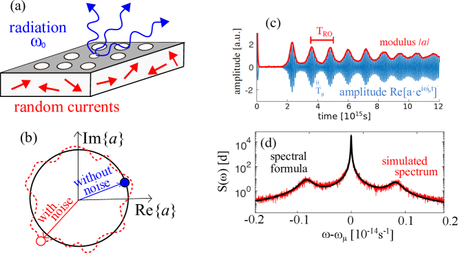
Figure 1: (a) A photonic-crystal laser cavity, with stimulated emission (blue) and spontaneous emission noise (red arrows). (b) Phasor diagram of the amplitude of a single-mode laser $a(t)$ [which obeys Eq. (6)]. Without noise, $a$ undergoes harmonic oscillations at the laser frequency $\omega_{\mu}$ (black), but in the presence of noise, $a$ exhibits small intensity fluctuations and large phase drifts (red). (c) Evolution of the rotated mode amplitude, $\mathrm{Re}[ae^{i\omega_{L}t}]$, (blue) and modulus, $|a|$, (red) from the initial state until reaching the steady state. The field amplitude oscillates at frequency $\omega_{\mu}$ while the modulus undergoes relaxation oscillations with frequency $\omega_{\mathrm{RO}}$. (d) Noise spectrum, obtained from the Fourier transform of the simulated solution of Eq. (6) (red) and by evaluating the spectral formula (black) [Eq. (7)].

Laser dynamics are surveyed in many sources [26, 27, 28, 29, 30], but it is useful to review here a simple physical picture of laser noise. A resonant cavity [e.g., light bouncing between two mirrors or a photonic-crystal (PhC) microcavity [31] as in Fig. 1(a)] traps light for a long time in some volume, and lasing occurs when a gain medium is “pumped" to a population “inversion" of excited states to the point (threshold) where gain balances loss. The nonlinear interaction between the field and the gain medium stabilizes the system at a steady state. If noise were absent, the field would perform harmonic oscillations and the laser-power spectrum would consist of delta functions at the oscillation frequencies, $\omega_{\mu}$. However, noise [represented by red arrows in panel (a)] is always present, and it “kicks” the field away from the steady state. Fluctuations in the intensity of the field are suppressed by the nonlinear interaction with the gain, while phase fluctuations can be large [see panel (b)]. The phase undergoes a Brownian motion, which leads to broadening of the central lasing peaks [15, 32]. The effect of intensity fluctuations depends on the relative relaxation rates of the gain and the field [33, 34, 35]. When the population inversion of the medium decays much more rapidly than the field (a regime called “class-A lasers”), intensity fluctuations decay exponentially to the steady state. A non-zero intensity-phase coupling leads to enhanced phase variance, which increases the linewidths of the central peaks by a factor of $1+\alpha^{2}$ [15, 16, 25] (where $\alpha$ is “the amplitude–phase coupling” and can be computed from the lasing mode and material properties [16, 25]). In the limit of comparable inversion and field relaxation rates (i.e., in “class-B lasers”), the inversion and laser intensity undergo relaxation oscillations (ROs) [29, 30], which produce, in addition to central-peak broadening, a series of sidepeaks in the noise spectrum [see panels (c–d), obtained by numerically solving Eq. (6) and Eq. (7), as explained below]. The amplitudes of subsequent peaks in the series decrease exponentially and, in most cases, only the first-order sidepeaks are measurable. Last, when fluctuations in the inversion relax much more slowly than the field (i.e., in “class-C lasers”), multimode lasing is unstable and the dynamics is chaotic [33]. This paper focuses on RO sidepeaks, which are relevant for class-B lasers.

RO sidepeaks were first predicted and measured by Vahala et al. [20, 36]. The early measurements found an asymmetry between the amplitudes of the blue and red sidepeaks [37, 38]. Later work by van Exter et al. [21] attributed this asymmetry to the $\alpha$ factor. Since most typical semiconductor lasers have a positive $\alpha$ factor [37, 38], this result implied that the red sidepeaks are usually stronger than blue sidepeaks (negative $\alpha$ factors are possible [25, 39], but are less common). The van Exter work used the traditional laser rate equations in order to derive the power-spectrum formula, but these rate equations were derived under severe approximations and, hence, limit the generality of this result. In this work, we remedy this shortcoming by using generalized rate equations [Eq. (6)], which treat the inhomogeneity and nonlinearity in the laser medium accurately. These equations were derived in Ref. 1, and are introduced in the next section.

2 From Langevin Maxwell–Bloch to the oscillator equations

The starting point of our derivation in Ref. 1 is the Langevin Maxwell–Bloch equations [27, 40], which describe the dynamics of an electromagnetic field ($\mathbf{E}$) interacting with a two-level gain medium, represented by polarization ($\mathbf{P}$) and population inversion (${D}$), in the presence of noise ($\mathbf{F}_{S}$):

$$\nabla\times\nabla\times\mathbf{E}+\varepsilon_{c}(\mathbf{x})\hskip 2.0pt\ddot{\mathbf{E}}=-\ddot{\mathbf{P}}+\mathbf{F}_{S}$$ (1a)

$$\dot{\mathbf{P}}=-i(\omega_{a}-i\gamma_{\perp})\mathbf{P}-i\gamma_{\perp}\mathbf{E}\,D$$ (1b)

$$\dot{D}=-\gamma_{\parallel}\left[D_{0}\,F(\mathbf{x})-D+\frac{i}{2}(\mathbf{E}\cdot\mathbf{P}^{*}-\mathbf{E}^{*}\cdot\mathbf{P})\right]$$ (1c)

The first equation is a Maxwell-type equation for the field in a cavity with passive permittivity $\varepsilon_{c}(\mathbf{x})$, which is driven by the atomic polarization and the noise. The second equation is an oscillator equation for the polarization, with frequency $\omega_{a}$ and damping rate $\gamma_{\perp}$, which is driven by the field and the inversion. Last, the inversion is created by an external pump source [with $D_{0}$ and $F(\mathbf{x})$ representing the pump strength and spatial distribution]; it is saturated by the field and atomic polarization, relaxing to the steady state at a rate $\gamma_{\parallel}$. Throughout the paper, we use bold letters to denote vectors. The units and underlying assumptions of this model are discussed in [41, 42, 43, 44]. Note that Eq. (1a) neglects spatial dispersion [45] (i.e., nonlocal effects), which may arise due to gain diffusion [46], e.g., in some molecular-gas [47] and semiconductor lasers [48]. Such effects will not alter the noise spectrum when the diffusion is much slower than the bare inversion relaxation rate $\gamma_{\parallel}$; the strong-diffusion regime is beyond the scope of this work. For simplicity of presentation, Eq. (1a) neglects also spectral dispersion (nonlocality in time) of the passive permittivity. However, our derivation of the noise spectrum is valid also for dispersive media, so we include a frequency dependence in the Fourier transform of $\varepsilon_{c}(\mathbf{x})$, which appears in Table 1.

Noise is incorporated by including a fluctuating current source, $\mathbf{F}_{S}$, in the equation for the field [Eq. (1a)], whose correlations are given by the FDT, under the assumption of local thermal equilibrium. Although lasers are pumped nonlinear systems, when operating at steady state, they reach thermal equilibrium [2, 3, 4, 13, 14] since dissipation by optical absorption must be balanced by spontaneous emission. The probability distribution of the atomic populations obeys Boltzmann statistics, with an effective inverse temperature defined as [49, 12, 50]

$$\beta(\mathbf{x})\equiv\frac{1}{\hbar\omega_{0}}\ln\left(\frac{N_{1}(\mathbf{x})}{N_{2}(\mathbf{x})}\right),$$ (2)

with $N_{1}$ and $N_{2}$ being the populations in the lower and upper states of the lasing transition. Under these conditions, one can apply the FDT to find the correlations of the noise [14]:

$$\left<\tilde{\mathbf{F}}_{S}(\mathbf{x},\omega)\tilde{\mathbf{F}}\textsuperscript{*}_{S}(\mathbf{x}^{\prime},\omega^{\prime})\right>=4\hbar\omega^{4}\mathrm{Im}\left[\varepsilon(\mathbf{x},\omega)\right]\coth\left(\frac{\hbar\omega\beta(\mathbf{x},\omega)}{2}\right)\delta(\mathbf{x}-\mathbf{x}^{\prime})\delta(\omega-\omega^{\prime}).$$ (3)

Here, $\varepsilon(\mathbf{x},\omega)$ is the dispersive permittivity of the laser, which includes nonlinear gain saturation above the lasing threshold [$\varepsilon$ is defined in Table 1 and by the square brackets in Eq. (5)]. The inverse temperature, $\beta$, and the imaginary part of the permittivity, $\mathrm{Im}[\varepsilon]$, are negative in gain regions (where the inversion $D\equiv N_{2}-N_{1}$ is positive) while both are positive elsewhere. In our approach (and also in  Refs. 16, 18, 19), $\mathbf{F}_{S}$ represents the fluctuating spontaneous emission field. An equivalent description of laser noise can be obtained by introducing fluctuating currents in the atomic variables [Eq. (1b) and Eq. (1c)], instead of $\mathbf{F}_{S}$, but we showed in Ref. 51 that the formulations are equivalent.

A recent advance in the theory of microstructured lasers [41, 42, 44] shows that in many cases, the Maxwell–Bloch equations can be greatly simplified: The inversion in most microlasers is nearly stationary and, therefore, there exists a stable steady-state solution of the form

$$\mathbf{E}(\mathbf{x},t)=\sum_{\mu}\mathbf{E}_{\mu}(\mathbf{x})a_{\mu 0}e^{-i\omega_{\mu}t}.$$ (4)

The Maxwell–Bloch equations can be reduced to a single Maxwell-type equation of the form

$$\left(\nabla\times\nabla\times-\omega_{\mu}^{2}\left[\varepsilon_{c}(\mathbf{x},\omega)+\frac{\gamma_{\perp}}{\omega_{\mu}-\omega_{a}+i\gamma_{\perp}}\frac{D_{0}\,F(\mathbf{x})}{1+\sum_{\nu}\frac{\gamma_{\perp}^{2}}{(\omega_{\nu}-\omega_{a})^{2}+\gamma_{\perp}^{2}}|a_{\nu 0}|^{2}|\mathbf{E}_{\nu}(\mathbf{x})|^{2}}\right]\right)\mathbf{E}_{\mu}(\mathbf{x})=0.$$ (5)

This is a dispersive nonlinear eigenvalue problem, whose solutions determine the steady-state lasing frequencies $\omega_{\mu}$, amplitudes $a_{\mu 0}$, and modes $\mathbf{E}_{\mu}(\mathbf{x})$, which can be found by employing numerical algorithms (as outlined in Ref. 52). The set of assumptions underlying the derivation of Eq. (5) are commonly abbreviated as SALT—the steady-state ab-initio laser theory.

When noise is introduced, the laser field can still be approximated by Eq. (4), but now the complex amplitudes, $a_{\mu}(t)$, vary over time. In Ref. 1, we derive dynamical equations for $a_{\mu}(t)$ by using numerical solutions of the SALT equation [Eq. (5)] while treating the effect of noise analytically. A weak noise causes small intensity fluctuations relative to the steady-state intensity i.e., $|a_{\mu}(t)|^{2}\approx|a_{\mu 0}|^{2}$ (this assumption breaks down near the lasing threshold). In the single-mode regime, we find

$$\dot{a}_{\mu}(t)=\int\!d\mathbf{x}\,c_{\mu\mu}(\mathbf{x})\gamma(\mathbf{x})\int^{t}\!\!dt^{\prime}e^{-\gamma(\mathbf{x})(t-t^{\prime})}\left(a_{\mu 0}^{2}-|a_{\mu}(t^{\prime})|^{2}\right)a_{\mu}(t)+f_{\mu}(t),$$ (6)

Quantity	Symbol	Definition
SALT permittivity	$\varepsilon(\mathbf{x},\omega)$	$\varepsilon_{c}(\mathbf{x},\omega)+\frac{\gamma_{\perp}D_{0}F(\mathbf{x})}{\omega-\omega_{a}+i\gamma_{\perp}}\left[1+\displaystyle\sum_{\mu}\frac{\gamma_{\perp}^{2}}{(\omega_{\mu}-\omega_{a})^{2}+\gamma_{\perp}^{2}}|a_{\mu 0}|^{2}|\mathbf{E}_{\mu}|^{2}\right]^{-1}$
Nonlinear restoring force	$c_{\mu\nu}(\mathbf{x})$	$\frac{-i\omega_{\mu}^{2}\tfrac{\partial\varepsilon(\mathbf{x},\omega_{\mu})}{\partial|a_{\nu 0}|^{2}}\mathbf{E}_{\mu}^{2}(\mathbf{x})}{\scalebox{0.9}{$\displaystyle\int\!dx\,\left.\tfrac{d}{d\omega}\left[\omega^{2}\varepsilon(\mathbf{x},\omega)\right]\right|_{\omega_{\mu}}\mathbf{E}_{\mu}^{2}(\mathbf{x})$}}$
Dressed decay rate	$\gamma(\mathbf{x})$	$\gamma_{\parallel}\left(1+\displaystyle\sum_{\mu}\frac{\gamma_{\perp}^{2}}{(\omega_{\mu}-\omega_{\mathrm{a}})^{2}+\gamma_{\perp}^{2}}\hskip 2.0pt|a_{\mu 0}|^{2}|\mathbf{E}_{\mu}(\mathbf{x})|^{2}\right).$
Noise amplitude	$R_{\mu\nu}(\omega)$	$2\hbar\omega_{\mu}^{4}\hskip 2.0pt\frac{\scalebox{0.9}{$\displaystyle\int\!\!dx\hskip 2.0pt{|\mathbf{E}_{\mu}(\mathbf{x})|}^{2}\mbox{Im}\hskip 2.0pt\varepsilon(\mathbf{x},\omega)\coth\left(\frac{\hbar\omega_{\mu}\beta(\mathbf{x},\omega)}{2}\right)$}}{{\left|\scalebox{0.9}{$\displaystyle\int\!dx\,\left.\tfrac{d}{d\omega}\left[\omega^{2}\varepsilon(\mathbf{x},\omega)\right]\right|_{\omega_{\mu}}\mathbf{E}_{\mu}^{2}(\mathbf{x})$}\right|}^{2}}\cdot\delta_{\mu\nu}$

Table 1: The coefficients of the single- and multi-mode generalized rate equations [Eq. (6) and Eq. (16)], expressed in terms of the laser parameters [cavity permittivity, $\varepsilon_{c}(x)$, gain frequency and bandwidth, $\omega_{a}$ and $\gamma_{\perp}$, and pump intensity and spatial profile, $D_{0}$ and $F(x)$] as well as the laser steady-state properties [SALT frequencies $\omega_{\mu}$, mode amplitudes, $a_{\mu 0}$, and mode profiles, $\mathbf{E}_{\mu}(\mathbf{x})$]. The definitions are borrowed from Ref. 1.

where the parameters $c_{\mu\mu}(\mathbf{x})$, $\gamma(\mathbf{x})$, and $a_{\mu 0}$ are obtained from SALT (as shown in Table 1) [1]. The nonlinear restoring force, $c_{\mu\mu}(\mathbf{x})$, can be thought of as an effective gain rate (being proportional to the product of the lasing frequency $\omega_{\mu}$ and pump amplitude $D_{0}$). The dressed relaxation rate, $\gamma(\mathbf{x})$, is a sum of the bare atomic-relaxation rate, $\gamma_{\parallel}$, and a nonlinear spatially-inhomogeneous term, which turns on at the lasing threshold. Last, the noise is represented by a random Langevin term, $f_{\mu}(t)$, and only its amplitude $R_{\mu\mu}$ [defined via $\langle f_{\mu}(t)f_{\mu}^{*}(t^{\prime})\rangle=R_{\mu\mu}\delta(t-t^{\prime})$] determines the (ensemble-averaged) noise spectrum. Treating spontanteous emission as white noise [15] (i.e., uncorrelated in time) is equivalent to assuming that the noise autocorrelation function [$R_{\mu\mu}(\omega)$] is nearly constant for frequencies within the lasing peaks. This assumption is valid when the lasing linewidths are much narrower than the gain bandwidth. The effect of colored noise can be incorporated into our approach, as mentioned in Sec. 5. A solution of Eq. (6) is shown in Fig. 1(c) for a particular realization of the noise process, $f_{\mu}(t)$, with parameters $a_{\mu}(0)=5,a_{\mu 0}=1,R_{\mu\mu}=1.44\cdot 10^{-4}\,s^{-1},\int\!\!d\mathbf{x}\,c_{\mu\mu}(\mathbf{x})=0.19+1.18i\,s^{-1}$ and a constant atomic-relaxation rate, $\gamma(\mathbf{x})=0.0025\,s^{-1}$ (which is a good approximation near threshold, because the nonlinear inhomogeneous term is much smaller than the bare rate). These parameters correspond to a type-B laser (i.e., with comparable atomic and light relaxation rates) and, indeed, the solution reveals RO dynamics. In Ref. 1, we used Eq. (6) to compute the central-peak linewidths. In this work, we use it to compute the entire noise spectrum, as shown in the next section.

3 The noise spectrum of single-mode lasers

3.1 Formula for the noise spectrum

Before diving into the details of the derivation of the single-mode formula (in Sec. 3.3), we summarize our results: the new formula, its validation, and its consequences. The noise spectrum of a single-mode laser with lasing-frequency $\omega_{\mu}$ is

$$S_{\mu}(\omega)=\underbrace{\frac{{\Gamma_{0}(\omega_{\mu})}(\alpha_{1}^{2}+1)}{(\omega-\omega_{\mu})^{2}+\left[\tfrac{{\Gamma_{0}(\omega_{\mu})}}{2}(\alpha_{1}^{2}+1)\right]^{2}}\left(1-\frac{{\Gamma_{0}(\omega_{\mu})}(\alpha_{2}^{2}+1)}{4\Gamma}\right)}_{\text{central peak}}+$$

$$\underbrace{\frac{{\Gamma_{0}(\omega_{\mu}-\Omega)}(\alpha_{2}^{2}+1)/4}{\Gamma_{\mathrm{SB}}^{2}+(\omega-\omega_{\mu}+\Omega)^{2}}\left(1+\frac{4\alpha_{3}}{\alpha_{2}^{2}+1}\cdot\frac{\Gamma}{\Omega}+\frac{3\alpha_{2}^{2}-1}{\alpha_{2}^{2}+1}\cdot\frac{\omega-\omega_{\mu}+\Omega}{\Omega}\right)}_{\text{red sideband}}+$$

$$\underbrace{\frac{{\Gamma_{0}(\omega_{\mu}+\Omega)}(\alpha_{2}^{2}+1)/4}{\Gamma_{\mathrm{SB}}^{2}+(\omega-\omega_{\mu}-\Omega)^{2}}\left(1-\frac{4\alpha_{3}}{\alpha_{2}^{2}+1}\cdot\frac{\Gamma}{\Omega}-\frac{3\alpha_{2}^{2}-1}{\alpha_{2}^{2}+1}\cdot\frac{\omega-\omega_{\mu}-\Omega}{\Omega}\right)}_{\text{blue sideband}}.$$ (7)

Quantity	Symbol	Definition
Phase diffusion coefficient	$\Gamma_{0}(\omega)$	$R_{\mu\mu}(\omega)/2a_{\mu 0}^{2}$
RO frequency	$\Omega$	$\left[2a_{0}^{2}\int\!d\mathbf{x}\,\mathrm{Re}\,c_{\mu\mu}(\mathbf{x})\gamma(\mathbf{x})\right]^{1/2}$
RO decay rate	$\Gamma$	$\int\!d\mathbf{x}\,\gamma(\mathbf{x})/2$
Sideband linewidth	$\Gamma_{\mathrm{SB}}$	$\Gamma_{0}(\alpha_{1}^{2}+1)+\Gamma$
Linewidth enhancement	$\alpha_{1}$	$\frac{\int\!d\mathbf{x}\,\mathrm{Im}\,[c_{\mu\mu}(\mathbf{x})]}{\int\!d\mathbf{x}\,\mathrm{Re}\,[c_{\mu\mu}(\mathbf{x})]}$
Sideband power fraction	$\alpha_{2}$	$\frac{\int\!d\mathbf{x}\,\gamma(\mathbf{x})\mathrm{Im}\,[c_{\mu\mu}(\mathbf{x})]}{\int\!d\mathbf{x}\,\gamma(\mathbf{x})\mathrm{Re}\,[c_{\mu\mu}(\mathbf{x})]}$
Asymmetry factor	$\alpha_{3}$	$\frac{\int\!d\mathbf{x}\,\gamma(\mathbf{x})^{2}\mathrm{Im}\,[c_{\mu\mu}(\mathbf{x})]}{\left[\int\!d\mathbf{x}\,\gamma(\mathbf{x})\mathrm{Re}\,[c_{\mu\mu}(\mathbf{x})]\right]\left[\int\!d\mathbf{x}\,\gamma(\mathbf{x})\right]}$

Table 2: Coefficients of the single-mode noise spectrum [Eq. (7)], expressed in terms of quantities obtained from SALT: the steady-state modal amplitudes, $a_{\mu 0}$, and the oscillator-equation coefficients, $c_{\mu\mu}(\mathbf{x})$, $\gamma(\mathbf{x})$, and $R_{\mu\mu}$, defined in Table 1.

The first term corresponds to the central Lorentzian peak, while the second and third terms are the red and blue RO sidepeaks. In Table 2, we express all the parameters from Eq. (7) in terms of the coefficients of the generalized rate equation [Eq. (6)]. For ease of notation, we omit the subscript $\mu$ from the coefficients. Since these coefficients are functions of the SALT solutions (as shown in Table 1), the evaluation of Eq. (7) requires no additional free parameters besides those appearing in the Maxwell–Bloch equations [Eq. (1)]. The central peak is centered around the SALT lasing frequency, $\omega_{\mu}$, and its linewidth is the product of the phase-diffusion coefficient, ${\Gamma_{0}}(\omega_{\mu})$, and the amplitude–phase-coupling enhancement factor, $\alpha_{1}^{2}+1$. Since some of the noise power goes into the sidepeaks, the amplitude of the central peak is reduced by a factor of $1-\tfrac{\Gamma_{0}(\omega_{\mu})}{4\Gamma}(1+\alpha_{2}^{2})$, where $\Gamma$ is the rate at which ROs decay and $\alpha_{2}$ is the second generalized phase–amplitude-coupling factor. The RO sidepeaks are Lorentzians, whose center-frequency and linewidth are $\omega_{\mu}\pm\Omega$ and $\Gamma_{\mathrm{SB}}$ respectively. The amplitude of the blue and lred sidepeaks differs by a factor of $\frac{4\alpha_{3}}{\alpha_{2}^{2}+1}$, where $\alpha_{3}$ is the third generalized amplitude–phase-coupling factor.

Our new formula [Eq. (7)] is formally similar to the result of Ref. 21, but here we obtain three kinds of generalized $\alpha$ factors, while in Ref. 21 they are the same. In Ref. 21, the $\alpha$ factoer is given by the traditional expression $\alpha_{1,2,3}=\frac{\mathrm{Re}[\Delta n]}{\mathrm{Im}[\Delta n]}$, where $\Delta n$ is the change in index of refraction following a noise-driven perturbation [15]. In contrast, our generalized $\alpha$ factors are spatial averages of the refractive index change with different weight factors (as defined in Table 2 and discussed in Sec. 3.2). While the parameters in our formula are obtained directly from the Maxwell–Bloch equations, the parameters in Ref. 21 are expressed in terms of many additional parameters (such as the mode volume, confinement factor, cold-cavity decay rate, effective differential gain, gain saturation coefficient, etc.) and, quantitatively, can only be obtained by empirical fits. Similar to previous work, our derivation of Eq. (7) assumes that $\Gamma\ll\Omega$, which implies that the sidepeaks have little overlap with the central lasing peak.

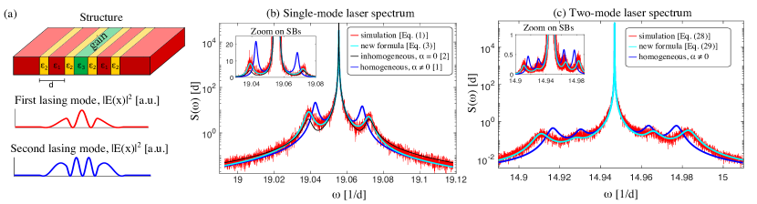
Figure 2: (a) Top: A periodic stack of layers with alternating permitivities ($\varepsilon_{1},\varepsilon_{2}$) and thicknesses ($d_{1},d_{2}$), with a defect layer (with $\varepsilon_{3}$ and $d_{3}$). The parameters (see text) are chosen such that the structure has two cold-cavity localized modes inside the band gap. Gain is added in the three central layers in order to make the gap modes lase. Bottom: Intensity profiles of the first and second lasing modes (with threshold frequencies $\omega_{1}=19.05$ and $\omega_{2}=14.95$ respectively). (b) Spectrum of a single-mode laser, on a log-linear scale, computed by time-stepping Eq. (6) (red) and by evaluating our single-mode formula [Eq. (7)] (cyan) and earlier results: [21] (black) which neglected $\alpha-$factor corrections and [1] (blue) which neglected inhomogeneity and nonlinearity of the modes and gain. Inset: Magnification of the sidepeaks, plotted on a linear scale, which shows the asymmetry of the peaks. (c) Spectrum of a multimode laser. We compare the numerical solution of the stochastic equations [Eq. (16)] (red) with our multimode formula [Eq. (17)] (cyan). Additionally, we plot the homogeneous limit of our formula (black) . Inset: Zoom on the sidepeaks.

3.2 Validation and main predictions of the formula

We validate our single-mode formula [Eq. (7)] by comparing it with brute-force simulations of the generalized rate equations [Eq. (6)] and with previous theories [1, 21] (Fig. 2). Since we expect Eq. (7) to deviate from the traditional results in the limit of substantially different $\alpha$ factors, we study a numerical example where the $\alpha$ factor can be easily tuned: A periodic array of dielectric slabs with a defect at the center of the structure and gain in the defect area (we discussed a similar structure in Ref. 1). Our motivation to study this structure is the fact that the traditional $\alpha$ factor is proportional to the detuning of the gain resonance from the lasing frequency [53]; since the frequency of the defect mode is unaltered by small changes in the gain, one can vary $\alpha$ by varying the resonance of the gain. The structure is shown in panel (a). The parameters are $\varepsilon_{1}=1,\varepsilon_{2}=16,\varepsilon_{3}=7,d_{1}=0.2a,d_{2}=\tfrac{\sqrt{\varepsilon_{1}}a}{\sqrt{\varepsilon_{1}}+\sqrt{\varepsilon_{2}}}=0.8a,d_{3}=0.2a,\gamma_{\parallel}=0.006,\omega_{a}=18$ and $\gamma_{\perp}=1$ in (b) [and $\omega_{a}=17$ and $\gamma_{\perp}=2$ in (c)]. Here, $a$ is the unit-cell size and the frequency unit is $2\pi c/a$. We employ a finite-difference frequency-domain (FDFD) [55, 56] approach to discretize the SALT equations, and use the algorithm from Ref. 52 to obtain the steady-state modes [$\mathbf{E}_{\mu}(\mathbf{x})$], frequencies ($\omega_{\mu}$), and amplitudes ($a_{\mu 0}$). Using these solutions, we compute the coefficients from Table 1, which we use both to evaluate our spectral formula [Eq. (7)] and as the starting point for numerical simulations of Eq. (6). The simulations include time-stepping of Eq. (6) (by implementing a standard Euler scheme for stochastic ordinary differential equations [57]) and taking the ensemble average of the Fourier transform of the mode intensity $|a_{\mu}|^{2}$ (also called the periodogram of the signal [58]).

The results are shown in panel (b). An important advantage of the new formulation is that it correctly accounts for the spatially dependent enhancement of the atomic relaxation rate, $\gamma(\mathbf{x})$, above the lasing threshold (defined in Table 1). This enhancement affects the sideband spectrum since both the oscillation frequency and sideband linewidth depend on $\gamma(\mathbf{x})$ (see Table 2). Previous treatments, which assumed either that the relaxation rate is independent of the field [36] or that it is constant (fixed at the unsaturated value) [21], underestimated the broadening and shifting of the sidepeaks. In Figs. 2(b–c), we demonstrate that our formula (cyan) matches the numerically simulated noise spectrum (red), while homogeneous models, which corresponds to assuming a bare relaxation rate (black) or an unsaturated rate (blue) fail.

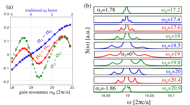
Figure 3: (a) Deviation of the generalized $\alpha$ factors ($\alpha_{1,2,3}$ in Table 2) from the traditional factor ($\alpha_{0}=\tfrac{\omega_{a}-\omega_{\mu}}{\gamma_{\perp}}$) for the structure from Fig. 2a. The plot shows the $\alpha$ factors at a fixed pump power for varying gain frequencies. Large deviations are evident for large detunings. Most notably, $\alpha_{3}$ deviates non-monotonically from $\alpha_{0}$ in the shown frequency range. (b) Sideband spectrum for gain-resonance frequencies in the range $\omega_{a}=17.2\ldots 21$. When $\alpha_{3}>0$, the red sidepeak are stronger than the blue sidepeak, and this picture is reversed when $\alpha_{3}<0$.

Figure 3(a) presents a comparison of the traditional and generalized amplitude–phase coupling factors. The traditional $\alpha$ factor was introduced by Lax [53], where he used a zero-dimensional model (which neglects inhomogeneity in the pump and the fields) to explain central-peak linewidth broadening in detuned-gas lasers. Ref. 53 shows that the amplitude–phase coupling is equal to the detuning of the lasing frequency from the atomic resonance, i.e., $\alpha_{0}=\frac{\omega_{0}-\omega_{\mathrm{a}}}{\gamma_{\perp}}$. Later work by Henry [15] found that in semiconductor lasers, the amplitude-phase coupling is $\tilde{\alpha}_{0}=\frac{\mathrm{Re}[\Delta n]}{\mathrm{Im}[\Delta n]}$, where $\Delta n$ is the change in index of refraction following a noise-driven perturbation. In Ref. 1, we showed that the Lax and Henry definitions are equivalent and that, more generally, the amplitude-phase coupling ($\alpha_{1}$) is given by the ratio of the spatial averages of the real- and imaginary-index fluctuations (see definition in Table 2). Moreover, we showed that the difference between the traditional and the generalized factors, $\alpha_{1}-\alpha_{0}$, increases with increasing $\alpha_{0}$. Motivated by this prediction, we present in Fig. 3(a) the deviation of the generalized $\alpha$ factors ($\alpha_{1},\alpha_{2},\alpha_{3}$) from the traditional $\alpha_{0}$ as a function of gain-center frequency $\omega_{a}$. We find that all three factors deviate substantially from $\alpha_{0}$ at large detunings. All the data points in the plot are obtained at a fixed pump power ($D_{0}=0.095$). The relaxation rates of the inversion and polarization are $\gamma_{\parallel}=0.006$ and $\gamma_{\perp}=1$, as in Fig. 2(b).

Figure 3(b) demonstrates the dependence the sideband asymmetry on the generalized factor $\alpha_{3}$. We compute the entire noise spectrum for several gain-center frequencies in the range $\omega_{a}-\omega_{\mu}\in(-1.8,2)$, with $\gamma_{\parallel}=0.02$, $\gamma_{\perp}=1$ and $D_{0}=0.095$. From Eq. (7), one can see that the asymmetry is controlled by $\alpha_{3}$. In this numerical example, $\alpha_{0}\approx 1$ and $\alpha_{3}$ differs from $\alpha_{0}$ by approximately $10\%$ [see Fig. 3(a)]. The traditional factor $\alpha_{0}$ changes sign when the gain frequency is equal to the lasing frequency, so we expect the asymmetry of the sidebands to change sign as we sweep the gain center frequency across the cavity resonance. This trend is evident in Fig. 3(b). Since $\alpha_{3}$ changes sign in the range $\omega_{0}-\omega_{\mathrm{a}}\in(0,1)$, the red sidepeaks are weaker than the blue sidepeaks, in contrast to the more common case of positive-$\alpha$ semiconductor lasers [25], where red sidebands are stronger.

3.3 Derivation outline

In this section, we outline the derivation of Eq. (7), leaving the detailed explanations to appendix A. Our derivation is inspired by the approach of Ref. 21, but since we use the ab-initio dynamical oscillator equations [Eq. (6)] instead of the traditional laser rate equations, our derivation is more involved and the results are more general. Our starting point is the Wiener–Khintchine theorem [59], which relates the laser-noise spectrum to the Fourier transform of the autocorrelation function $\left<a(t)a^{*}(0)\right>$ [where angle brackets denote an ensemble average over realizations of the noise process]. Since intensity and phase fluctuations have distinct roles in determining the noise spectrum (as explained in the introduction), it is convenient to write the complex mode amplitude, $a$, in the form [32]:

$$a(t)=a_{0}e^{-u(t)+i\phi(t)},$$ (8)

The autocorrelation of $a$ can be written as:

$$\frac{\langle a(t)a^{*}(0)\rangle}{\langle|a(0)|^{2}\rangle}=\langle\exp\left\{-\left[u(t)+u(0)\right]+i\left[\phi(t)-\phi(0)\right]\}\right\}\rangle/\langle\exp{[-2\langle u(0)\rangle]}\rangle\approx$$

$$\exp\scalebox{1.5}{$\{$}-\underbrace{\tfrac{\langle[\phi(t)-\phi(0)]^{2}\rangle}{2}}_{\text{phase variance}}\,+\!\underbrace{\tfrac{\langle[u(t)+u(0)]^{2}\rangle}{2}\rangle}_{\text{intensity correlations}}-i\underbrace{\langle[u(t)+u(0)][\phi(t)-\phi(0)]\rangle}_{\text{cross term}}\scalebox{1.5}{$\}$}/\langle\exp{[-2\langle u(0)\rangle]}.$$ (9)

The approximation in going from the first to second line can be justified as follows: First, we expand the exponent in a Taylor series. Since intensity fluctuations are smaller than the steady-state intensity, all the terms involving $u$ are small and we keep only the leading-order terms in the expansion. The phase variance [i.e., the $\phi^{2}$ term, given explicitly in Eq. (15a) below] is the sum of a “Brownian drift” term that grows linearly with time and a small RO term. The phase drift is the result of a Wiener (Brownian-motion) process of many uncorrelated spontaneous-emission “kicks” and, from the central-limit theorem  [60, 61], it follows that it is a Gaussian variable. The RO term is small and we keep only the corresponding leading term in the expansion. With these assumptions, we can move the ensemble average from the second equality on the first line inside the exponent and obtain the second line. This step is exact for log-normal distributions [62] (i.e., the exponent of a Gaussian phase), while it is a very good approximation for small fluctuations. Previous authors used a similar identity [19, 63], but incorrectly justified it by saying that all the variables are Gaussian, while clearly $u$ and $\phi$ are not Gaussian because they perform relaxation oscillations.

In order to relate the autocorrelation, $\langle a^{*}(t)a(0)\rangle$, to the steady-state laser properties, we need to obtain explicit expressions for the second-order moments: the phase variance, the intensity autocorrelation, and the cross term, defined in Eq. (9). To this end, we substitute Eq. (8) into Eq. (6) and linearize the resulting expression by assuming that intensity fluctuations are small compared to the steady-state intensity (i.e., $|u|\ll 1$). (Note that by linearizing the equations, we lose the higher-order RO peaks, but obtain accurate formulas for the first-order sidepeaks.) This procedure yields

$$\dot{\phi}(t)=\int\!d\mathbf{x}\,B(\mathbf{x})\xi(\mathbf{x},t)+f_{I}(t)/a_{0}\,,$$ (10a)

$$\dot{u}(t)=-\int\!d\mathbf{x}\,A(\mathbf{x})\xi(\mathbf{x},t)+f_{R}(t)/a_{0}\,,$$ (10b)

$$\dot{\xi}(\mathbf{x},t)=-\gamma(\mathbf{x})\xi(\mathbf{x},t)+\gamma(\mathbf{x})u(t)\,,$$ (10c)

where we introduced the time-delayed intensity fluctuation, $\xi(\mathbf{x},t)\equiv\int^{t}\!\!dt^{\prime}e^{-\gamma(\mathbf{x})(t-t^{\prime})}u(t^{\prime})$, in order to turn the integro-differential equations into a set of ordinary-differential equations (ODEs) [1]. We also introduced $A(\mathbf{x})$ and $B(\mathbf{x})$ to denote the real and imaginary parts of the nonlinear restoring force $2a_{0}^{2}c(\mathbf{x})$, and $f_{R}(t)$ and $f_{I}(t)$ are the real and imaginary parts of the Langevin noise term. We proceed by taking the Fourier transform of the linearized equations [Eq. (10)]. We solve the frequency-domain equations and obtain

$$\tilde{u}(\omega)=\frac{1}{i\omega+\int\!\!d\mathbf{x}\frac{A(\mathbf{x})\gamma(\mathbf{x})}{\gamma(\mathbf{x})+i\omega}}\cdot\frac{\tilde{f}_{R}(\omega)}{a_{0}}$$ (11a)

$$\tilde{\xi}(\mathbf{x},\omega)=\frac{\gamma(\mathbf{x})}{\gamma(\mathbf{x})+i\omega}\cdot\frac{1}{i\omega+\int\!\!d\mathbf{x}\frac{A(\mathbf{x})\gamma(\mathbf{x})}{\gamma(\mathbf{x})+i\omega}}\cdot\frac{\tilde{f}_{R}(\omega)}{a_{0}}$$ (11b)

$$\tilde{\phi}(\omega)=\frac{\int\!\!dx\tfrac{\gamma(x)B(x)}{\gamma(x)+i\omega}\cdot}{i\omega+\int\!\!dx\frac{A(x)\gamma(x)}{\gamma(x)+i\omega}}\cdot\frac{\tilde{f}_{R}(\omega)}{i\omega a_{0}}+\frac{\tilde{f}_{I}(\omega)}{i\omega a_{0}},$$ (11c)

As shown in appendix A, the time-dependent second-order moments can be written in terms of integrals over the power spectral densities [16]

$$\left<[\phi(t)-\phi(0)]^{2}\right>=\frac{1}{2\pi}\iint_{-\infty}^{\infty}{d}\omega{d}\omega^{\prime}\,\left<\tilde{\phi}(\omega)\tilde{\phi}^{*}(\omega^{\prime})\right>(1-e^{i\omega t})(1-e^{-i\omega^{\prime}t}),$$ (12a)

$$\left<[u(t)+u(0)]^{2}\right>=\frac{1}{2\pi}\iint_{-\infty}^{\infty}{d}\omega{d}\omega^{\prime}\,\left<\tilde{u}(\omega)\tilde{u}^{*}(\omega^{\prime})\right>(1+e^{i\omega t})(1+e^{-i\omega^{\prime}t}),$$ (12b)

$$\left<[\phi(t)-\phi(0)][u(t)+u(0)]\right>=\frac{1}{2\pi}\iint_{-\infty}^{\infty}{d}\omega{d}\omega^{\prime}\,\left<\tilde{\phi}(\omega)\tilde{u}^{*}(\omega^{\prime})\right>(1-e^{i\omega t})(1+e^{-i\omega^{\prime}t}).$$ (12c)

Since the integrands are meromorphic functions, these integrals can be computed by invoking the Cauchy residue theorem [64], which relates the integrals to the residues and poles of the integrands. The pole of $\tilde{\phi}$ at $\omega=0$ produces the central-peak linewidth, which we computed in Ref. 1. In order to see the remaining poles more clearly, we introduce the approximation:

$$\frac{1}{i\omega+\int\!\!d\mathbf{x}\frac{A(\mathbf{x})\gamma(\mathbf{x})}{\gamma(\mathbf{x})+i\omega}}=\frac{1}{\int\!\!d\mathbf{x}\frac{\left[i\omega(\gamma(\mathbf{x})+i\omega)+A(\mathbf{x})\gamma(\mathbf{x})\right]}{\gamma(\mathbf{\mathbf{x}})+i\omega}}\approx\frac{i\omega}{\int\!\!d\mathbf{x}\left[i\omega(\gamma(\mathbf{x})+i\omega)+A(\mathbf{x})\gamma(\mathbf{x})\right]}.$$ (13)

In the last equality, we assumed that $\gamma(\mathbf{x})+i\omega\approx i\omega$ for all $\mathbf{x}$, which holds near the RO frequencies in the limit of resolved sidepeaks, that is, for $\omega\approx\Omega\gg\Gamma$, using the definitions

$$\int\!\!d\mathbf{x}\left[i\omega(\gamma(\mathbf{x})+i\omega)+A(\mathbf{x})\gamma(\mathbf{x})\right]=-\omega^{2}+i\omega\scalebox{0.9}{$\left[\int\!\!d\mathbf{x}\,\gamma(\mathbf{x})\right]$}+\scalebox{0.9}{$\left[\int\!\!d\mathbf{x}A(\mathbf{x})\gamma(\mathbf{x})\right]$}\equiv-\omega^{2}+2i\omega\Gamma+\Omega^{2}.$$ (14)

From Eq. (14), one can see that the denominator of Eq. (13) is a second-degree polynomial that vanishes at $\pm\Omega+i\Gamma$ (in the limit of $\Omega\gg\Gamma$). These zeros produce the RO sidepeaks in the noise spectrum. By collecting the results, we find

$$\left<[\phi(t)-\phi(0)]^{2}\right>=\tfrac{R_{0}}{a_{0}^{2}}\left(1+\alpha_{1}^{2}\right)t+\tfrac{R_{\pm}\alpha_{2}^{2}}{2a_{0}^{2}\Gamma}(1-e^{-\Gamma t}\cos\Omega t)-\tfrac{3R_{\pm}\alpha_{2}^{2}}{2a_{0}^{2}\Omega}e^{-\Gamma t}\sin\Omega t$$ (15a)

$$\left<[u(t)+u(0)]^{2}\right>=\frac{R_{\pm}}{2\Gamma a_{0}^{2}}(1+\cos\Omega te^{-\Gamma t})+\frac{R_{\pm}}{2\Omega a_{0}^{2}}\sin\Omega te^{-\Gamma t}$$ (15b)

$$\left<[\phi(t)-\phi(0)][u(t)+u(0)]\right>=\tfrac{R_{0}\,\alpha_{1}}{a_{0}^{2}\,A}+\tfrac{R_{\pm}\,\alpha_{3}}{a_{0}^{2}\Omega}\left(-\tfrac{2\Gamma}{\Omega}\cos\Omega t\,e^{-\Gamma t}+\sin\Omega t\,e^{-\Gamma t}\right),$$ (15c)

where $A\equiv\int\!dx\,A(\mathbf{x})$ and all the parameters are defined in Table 2. We denote by $R_{0}$ and $R_{\pm}$ the autocorrelation evaluated at the lasing and RO frequencies respectively, i.e., $R(\omega_{\mu})$ and $R(\omega_{\mu}\pm\Omega)$. While the phase variance [Eq. (15a)] grows linearly in time, the intensity autocorrelation and the cross term [(15b,15c)] do not show diffusive behavior, which is expected because the nonlinear restoring force in the oscillator equations [Eq. (6)] prevents intensity drift.

After obtaining closed-form expressions for the second-order moments [Eq. (15)], we substitute these results into the autocorrelation [Eq. (9)] and take the Fourier transform to obtain the noise spectrum. The calculation can be simplified when the central peak in the spectrum is much narrower than the sidebands [which holds when all the coefficients in Eq. (15) (i.e., $R_{0}(1+\alpha_{1}^{2}),R_{\pm}\alpha_{2}^{2}$, etc.) are much smaller than $\Gamma$]. In this regime, we can expand the exponentials in Eq. (9) in a Taylor series around $R_{\pm}/\Gamma$ and obtain Eq. (7).

4 Noise spectrum of multimode lasers

We generalize our approach from Sec. 3.3 and obtain a formula for the multimode noise spectrum. In this section, we present our result, and the derivation details are given in appendix B. The starting point of the derivation is the multimode dynamical equations for the complex amplitudes $a_{\mu}$ [defined in Eq. (4)], which were derived in Ref. 1:

$$\dot{a}_{\mu}(t)=\sum_{\nu}\int\!d\mathbf{x}\,c_{\mu\nu}(\mathbf{x})\left[\gamma(\mathbf{x})\int^{t}\!\!dt^{\prime}e^{-\gamma(\mathbf{x})(t-t^{\prime})}\left(a_{\nu 0}^{2}-|a_{\nu}(t^{\prime})|^{2}\right)\right]a_{\mu}(t)+f_{\mu}(t),$$ (16)

where $\mu,\nu=1\ldots M$, for $M$ lasing modes. In Ref. 1, we used Eq. (16) to obtain the linewidths of the central lasing peaks. In appendix B, we complete the derivation of the multimode sidepeaks and find that the Fourier transform of the autocorrelation $\langle a_{\mu}(t)a^{*}_{\nu}(t^{\prime})\rangle$ is

$$S_{\mu\nu}(\omega)=\underbrace{\frac{\Gamma_{\mu\nu}}{(\omega-\omega_{\mu})^{2}+(\Gamma_{\mu\nu}/2)^{2}}\left(1-\frac{\sum_{\sigma}{[\mathbb{S}^{\sigma}_{\mu\nu}+\mathbb{U}^{\sigma}_{\mu\nu}]}}{2}\right)}_{\text{central peaks}}+$$

$$\underbrace{\scalebox{0.9}{$\displaystyle\sum_{\sigma}\frac{\Gamma^{\mu\nu\sigma}_{\mathrm{SB}}}{(\omega-\omega_{\mu}+\Omega_{\sigma})^{2}+{(\Gamma^{\mu\nu\sigma}_{\mathrm{SB}})}^{2}}\left[\left(\frac{\mathbb{S}^{\sigma}_{\mu\nu}+\mathbb{U}^{\sigma}_{\mu\nu}+2\mathbb{Y}^{\sigma}_{\mu\nu}}{2}\right)+\frac{\Omega_{\sigma}+\omega-\omega_{\mu}}{\Gamma_{\mathrm{SB}}}\left(\frac{\mathbb{V}^{\sigma}_{\mu\nu}-\mathbb{T}^{\sigma}_{\mu\nu}+2\mathbb{X}^{\sigma}_{\mu\nu}}{2}\right)\right]$}}_{\text{blue sidepeaks}}$$

$$\underbrace{\scalebox{0.9}{$+\displaystyle\sum_{\sigma}\frac{\Gamma^{\mu\nu\sigma}_{\mathrm{SB}}}{(\omega-\omega_{\mu}-\Omega_{\sigma})^{2}+{(\Gamma^{\mu\nu\sigma}_{\mathrm{SB}})}^{2}}\left[\left(\frac{\mathbb{S}^{\sigma}_{\mu\nu}+\mathbb{U}^{\sigma}_{\mu\nu}-2\mathbb{Y}^{\sigma}_{\mu\nu}}{2}\right)-\frac{\Omega_{\sigma}-\omega+\omega_{\mu}}{\Gamma_{\mathrm{SB}}}\left(\frac{\mathbb{V}^{\sigma}_{\mu\nu}-\mathbb{T}^{\sigma}_{\mu\nu}+2\mathbb{X}^{\sigma}_{\mu\nu}}{2}\right)\right]$}}_{\text{red sidepeaks}}.$$ (17)

Table 3: Coefficients of the multimode formula [Eq. (17)].

$A_{\mu\nu}(x)=2a_{\mu 0}a_{\nu 0}\mathrm{Re}[c_{\mu\nu}(x)],\quad\mathbb{A}=\int\!\!dx\,\mathbb{A}(x)$	$\mathbb{Q}_{+\sigma}=\displaystyle\sum_{\ell{m}{n}}\frac{\mathbb{P}_{+\sigma}\mathbb{P}_{-{n}}\mathbb{R}_{+}\mathbb{P}_{-\ell}^{\dagger}\mathbb{P}_{+{m}}^{\dagger}}{(\omega_{+\sigma}-\omega_{-{n}})(\omega_{+\sigma}-\omega_{+\ell}^{*})(\omega_{+\sigma}-\omega_{-{m}}^{*})}$
$B_{\mu\nu}(x)=2a_{\mu 0}a_{\nu 0}\mathrm{Im}[c_{\mu\nu}(x)],\quad\mathbb{B}=\int\!\!dx\,\mathbb{B}(x)$	$\mathbb{Q}_{-\sigma}=\displaystyle\sum_{\ell{m}{n}}\frac{\mathbb{P}_{+{n}}\mathbb{P}_{-\sigma}\mathbb{R}_{-}\mathbb{P}_{-\ell}^{\dagger}\mathbb{P}_{1{m}}^{\dagger}}{(\omega_{-\sigma}-\omega_{+{n}})(\omega_{-\sigma}-\omega_{+\ell}^{*})(\omega_{-\sigma}-\omega_{+{m}}^{*})}$
$\mathbb{M}_{\pm}\equiv\pm\sqrt{\int\!\!dx\mathbb{A}(x)\gamma(x)}+\frac{i}{2}\int\!\!dx\,\gamma(x)\,\mathbb{1}$	$\mathbb{S}^{\sigma}=\mathrm{Re}\tfrac{2i}{a_{0}^{2}}\scalebox{0.9}{$\left[\int\!\!dx\,\gamma(x)\mathbb{B}(x)\right]$}\left(\tfrac{\mathbb{Q}_{+\sigma}}{\omega_{+\sigma}^{2}}+\tfrac{\mathbb{Q}_{-\sigma}}{\omega_{-\sigma}^{2}}\right)\scalebox{0.9}{$\left[\int\!\!dx\,\gamma(x)\mathbb{B}(x)\right]^{T}$}$
$(\omega\mathbb{1}-\mathbb{M}_{\pm})^{-1}=\displaystyle\sum_{\sigma}\frac{\mathbb{P}_{\pm{\sigma}}}{\omega-\omega_{\pm\sigma}}$	$\mathbb{T}^{\sigma}=-\mathrm{Im}\tfrac{2i}{a_{0}^{2}}\scalebox{0.9}{$\left[\int\!\!dx\,\gamma(x)\mathbb{B}(x)\right]$}\left(\tfrac{\mathbb{Q}_{+\sigma}}{\omega_{+\sigma}^{2}}-\tfrac{\mathbb{Q}_{-\sigma}}{\omega_{-\sigma}^{2}}\right)\scalebox{0.9}{$\left[\int\!\!dx\,\gamma(x)\mathbb{B}(x)\right]^{T}$}$
$\omega_{\pm\sigma}=\pm\Omega_{\sigma}-i\Gamma_{\sigma}$	$\mathbb{U}^{\sigma}=\mathrm{Re}\left(\tfrac{2i}{a_{0}^{2}}\omega_{+\sigma}^{2}\mathbb{Q}_{+\sigma}+\omega_{-\sigma}^{2}\mathbb{Q}_{-\sigma}\right)$
$\Gamma_{\mu\nu}\equiv\tfrac{2[\mathbb{R}_{0}]_{\mu\mu}\delta_{\mu\nu}}{a_{\mu 0}a_{\nu 0}}+\tfrac{2(\mathbb{B}\mathbb{A}^{-1}\mathbb{R}_{0}{\mathbb{A}^{\dagger}}^{-1}\mathbb{B}^{\dagger})_{\mu\nu}}{a_{\mu 0}a_{\nu 0}}$	$\mathbb{V}^{\sigma}=-\mathrm{Im}\tfrac{2i}{a_{0}^{2}}\left(\omega_{+\sigma}^{2}\mathbb{Q}_{+\sigma}-\omega_{-\sigma}^{2}\mathbb{Q}_{-\sigma}\right)$
$\Gamma^{\mu\nu\sigma}_{\mathrm{SB}}\equiv\frac{\Gamma_{\mu\nu}}{2}+\Gamma_{\sigma}$	$\mathbb{X}^{\sigma}=\left[\int\!dx\,\gamma(x)^{2}\mathbb{B}(x)\right]\tfrac{\mathbb{Q}_{+\sigma}}{\omega_{+\sigma}}+\tfrac{\mathbb{Q}_{-\sigma}}{\omega_{-\sigma}}$
	$\mathbb{Y}^{\sigma}=2i\scalebox{0.9}{$\left[\displaystyle\int\!dx\,\gamma(x)^{2}\mathbb{B}(x)\right]$}\tfrac{\mathbb{Q}_{+\sigma}}{\omega_{+\sigma}}-\tfrac{\mathbb{Q}_{-\sigma}}{\omega_{-\sigma}}$

For convenience, we summarize all the coefficients of Eq. (17) in Table 3. Similar to Eq. (7), the first term represents the central peaks, which are Lorentzians at the lasing-mode frequencies $\omega_{\mu}$, whose widths $\Gamma_{\mu\mu}$ were derived in Ref. 1. The second and third terms correspond to the $2M$ red and blue sidepeaks, associated with each lasing mode. In contrast to the single-mode higher-order RO sidepeaks (mentioned above), which have exponentially decreasing intensities, the extra peaks in the multimode case have comparable amplitudes and should be measurable using standard experimental setups [20]. The RO frequencies and relaxation rates ($\Omega_{\sigma}$ and $\Gamma_{\sigma}$ respectively) are obtained from the real and imaginary parts of the complex eigenvalues of the matrix $\mathbb{M}$ (denoted by $\omega_{\pm\sigma}$, with $\sigma=1\ldots M$) . While $\Omega_{\sigma}$ determine the location of the RO peaks, $\Gamma_{\sigma}$ determine their linewidths, as can be seen from the definition of $\Gamma^{\mu\nu\sigma}_{\mathrm{SB}}$ in Table 3. The projectors onto the eigenvectors of $\mathbb{M}_{\pm}$, which we label in the table by $\mathbb{P}_{\pm\sigma}$, determine the multimode generalized $\alpha$ factors, which are expressed in terms of the matrices $\mathbb{S}^{\sigma},\mathbb{T}^{\sigma},\mathbb{U}^{\sigma},\mathbb{V}^{\sigma},\mathbb{X}^{\sigma}$ and $\mathbb{Y}^{\sigma}$. Even though our derivation requires many pages of algebra, we compare the final result to numerical solution of the nonlinear oscillator equations [Eq. (16)] and the results match perfectly [Fig. 2(c)].

5 Discussion

This paper presented an ab-initio formula for the noise spectrum of single- and multimode micro-structured complex-cavity lasers. Our results are valid under very general conditions: ($i$) the laser having a stationary inversion and reaching a stable steady state, ($ii$) operating far enough above the lasing threshold (so that intensity fluctuations in each mode are significantly smaller than the steady-state intensity), ($iii$) assuming that all the lasing peaks and sidebands are spectrally separated, and ($iv$) that spontaneous emission events are uncorrelated in time, which means that the noise autocorrelation function is treated as a constant within the spectral peaks (i.e., as white noise). As such, our theory is fairly general and accurately accounts for inhomogeneity, cavity openness, nonlinearity, and multimode effects in generic laser geometries. Since our formulas are expressed in terms of the steady-state lasing modes and frequencies, their evaluation does not require substantial computation beyond solving the steady-state SALT equations (which can be solved efficiently using available algorithms [41, 52]).

We find a number of new effects, which arise from the inhomogeneity of the lasing modes. For example, we find enhanced smearing and shifting of the RO sidepeaks in comparison to the traditional formulas (as demonstrated in Fig. 2), which follow from the spatial dependence of the effective atomic-relaxation rate, $\gamma(\mathbf{x})$, above the lasing threshold. Additionally, we obtain three generalized $\alpha$ factors: the central-peak linewidth-enhancement factor, $\alpha_{1}$ (which was already presented in Ref. 1), the fractional power that goes into the sidepeaks, $\alpha_{2}$, and the sideband-asymmetry factor, $\alpha_{3}$. We find that $\alpha_{1}$ is always larger than the traditional factor, $\alpha_{0}$, while $\alpha_{2}$ and $\alpha_{3}$ can be either larger or smaller than the traditional $\alpha_{0}$ (Fig. 3). The generalized factors ($\alpha_{1,2,3}$) deviate significantly from the the traditional factor ($\alpha_{0}$) in lasers with strong inhomogeniety, like random lasers  [65, 66] or lasers operating far above the threshold (where saturation effects become important).

The theory in this paper can be applied to tackle additional open questions in laser noise. For example, our current formulation treats only the effect of noise on the modes above the lasing threshold, but understanding the noise spectrum near and slightly below the threshold is very important, e.g., in the study of light-emitting diodes (LEDs). Although there have been previous attempts to describe laser noise near the threshold [67], the early theories use phenomenological rate equations for the lasing-mode amplitudes and artificially interpolate the sub-threshold and above-threshold regimes. Along these lines, one could interpolate Eq. (6) with the corresponding sub-threshold equation and easily obtain an improvement over previous work, since the latter uses phenomenological rate equations while our generalized equations are obtained directly from Maxwell–Bloch. Another effect that could potentially be treated using our FDT-based approach, is the regime of strong amplified spontaneous emission (ASE), where noise from near-threshold modes can affect the steady-state lasing properties, i.e., by suppressing lasing due to taking up the gain. We anticipate that strong ASE could be treated by introducing an ensemble-averaged steady-state inversion, in which noise from near-threshold modes would appear as an additional term in the gain saturation, where noise correlations are related to the steady-state properties of the medium by the FDT. Additionally, one could straightforwardly generalize our approach to include correlations between spontanteous emission events [relaxing assumption ($iv$) above], i.e., treat the random currents in Eq. (1a) as colored noise. In the application of the residue theorem in the appendices, one would need to include residues that correspond to the poles of $R_{\mu\nu}(\omega)$, which are neglected in the current analysis. These directions are further discussed in Ref. 68.

Funding

This work was partially supported by the Army Research Office through the Institute for Soldier Nanotechnologies under Contract No. W911NF-13-D-0001. AP is partially supported by an Aly Kaufman Fellowship at the Technion.

Appendix A: Derivation of the single-mode noise spectrum

In this appendix, we complete the derivation of Eq. (7) from the main text. After reviewing some definitions from the main text in Sec. A.1, we calculate the second-order moments of $u(t)$ and $\phi(t)$ in Sec. A.2. Then, in Sec. A.3, we use these results to obtain the power spectrum.

A.1. Autocorrelations of the single-mode phase and intensity

Recall that the Fourier transforms of $u(t)$, $\phi(t)$, and $\xi(t)$ are [Eq. (11)]:

$$\tilde{\phi}(\omega)=\frac{1}{i\omega+\int\!\!dx\frac{A(x)\gamma(x)}{\gamma(x)+i\omega}}\cdot\int\!\!dx\tfrac{\gamma(x)B(x)}{\gamma(x)+i\omega}\cdot\frac{\tilde{f}_{R}}{i\omega a_{0}}+\frac{\tilde{f}_{I}(\omega)}{i\omega a_{0}},$$ (A.1a)

$$\tilde{u}(\omega)=\frac{1}{i\omega+\int\!\!dx\frac{A(x)\gamma(x)}{\gamma(x)+i\omega}}\cdot\frac{\tilde{f}_{R}}{a_{0}},$$ (A.1b)

$$\tilde{\xi}(x,\omega)=\frac{\gamma(x)}{\gamma(x)+i\omega}\cdot\frac{1}{i\omega+\int\!\!dx\frac{A(x)\gamma(x)}{\gamma(x)+i\omega}}\cdot\frac{\tilde{f}_{R}}{a_{0}},$$ (A.1c)

where Fourier transforms are defined using the convention: $\tilde{f}\equiv\frac{1}{\sqrt{2\pi}}\int_{-\infty}^{\infty}\!\!dt\,e^{-i\omega t}f(t)$ [64]. Since intensity and phase are stationary random variables, the fluctuations at different frequencies are uncorrelated [16]

$$\langle\tilde{\phi}(\omega)\tilde{\phi}^{*}(\omega^{\prime})\rangle=R_{\tilde{\phi}\tilde{\phi}}(\omega)\delta(\omega-\omega^{\prime}),$$ (A.2a)

$$\langle\tilde{u}(\omega)\tilde{u}^{*}(\omega^{\prime})\rangle=R_{\tilde{u}\tilde{u}}(\omega)\delta(\omega-\omega^{\prime}),$$ (A.2b)

$$\langle\tilde{\phi}(\omega)\tilde{u}^{*}(\omega^{\prime})\rangle=R_{\tilde{\phi}\tilde{u}}(\omega)\delta(\omega-\omega^{\prime}).$$ (A.2c)

Given the autocorrelation of the Langevin noise $f$

$$\langle\tilde{f}(\omega)\tilde{f}^{*}(\omega)\rangle=R(\omega)\delta(\omega-\omega^{\prime}),$$ (A.3)

[with $R$ given by the fluctuation dissipation theorem (in Table 1)], and the explicit expressions for the Fourier transforms [Eq. (A.1)], we obtain

$$R_{\tilde{\phi}\tilde{\phi}}(\omega)=\left(1+\left|\tfrac{\int\!\!dx\tfrac{\gamma(x)B(x)}{\gamma(x)+i\omega}}{i\omega+\int\!\!dx\frac{A(x)\gamma(x)}{\gamma(x)+i\omega}}\right|^{2}\,\right)\cdot\frac{R(\omega)}{\omega^{2}a_{0}^{2}},$$ (A.4a)

$$R_{\tilde{u}\tilde{u}}(\omega)=\frac{1}{\left|i\omega+\int\!\!dx\frac{A(x)\gamma(x)}{\gamma(x)+i\omega}\right|^{2}}\cdot\frac{R(\omega)}{a_{0}^{2}},$$ (A.4b)

$$R_{\tilde{u}\tilde{\phi}}(\omega)=\frac{\int\!\!dx\frac{\gamma(x)B(x)}{\gamma(x)+i\omega}}{\left|i\omega+\int\!\!dx\frac{A(x)\gamma(x)}{\gamma(x)+i\omega}\right|^{2}}\cdot\frac{R(\omega)}{i\omega a_{0}^{2}}.$$ (A.4c)

In the text we, show that the noise spectrum depends on the poles of the autocorrelations in Eq. (A.1). In order to find these poles, we introduce the approximation [Eq. (13)]:

$$\frac{1}{i\omega+\int\!\!dx\frac{A(x)\gamma(x)}{\gamma(x)+i\omega}}\approx\frac{i\omega}{\int\!\!dx\left[i\omega(\gamma(x)+i\omega)+A(x)\gamma(x)\right]}=\frac{-i\omega}{(\omega-\omega_{+})(\omega-\omega_{-})},$$ (A.5)

which holds near the RO frequencies (i.e., when $\omega\approx\Omega\gg\Gamma$). Using this approximation, one finds that the autocorrelations have poles at the complex RO frequencies

$$\omega_{\pm}\equiv\pm\Omega+i\Gamma,$$ (A.6)

where

$$\Omega\equiv\scalebox{0.9}{$\sqrt{\int dxA(x)\gamma(x)}$},\quad\quad\quad\Gamma\equiv\scalebox{0.9}{$\frac{1}{2}\int dx\gamma(x)$}.$$ (A.7)

Using Eq. (A.5) and $\pm i\omega+\gamma(x)\approx\pm i\omega$, we find that the autocorrelations near the RO frequencies are:

$$R_{\tilde{\phi}\tilde{\phi}}(\omega)\approx\frac{R(\omega)}{\omega^{2}a_{0}^{2}}+\left|\frac{\int\!\!dx\tfrac{\gamma(x)B(x)}{\gamma(x)+i\omega}}{(\omega-\omega_{+})(\omega-\omega_{-})}\right|^{2}\frac{R(\omega)}{a_{0}^{2}},$$ (A.8a)

$$R_{\tilde{u}\tilde{u}}(\omega)\approx\frac{\omega^{2}}{\left|(\omega-\omega_{+})(\omega-\omega_{-})\right|^{2}}\cdot\frac{R(\omega)}{a_{0}^{2}},$$ (A.8b)

$$R_{\tilde{u}\tilde{\phi}}(\omega)\approx\frac{\omega^{2}\int\!\!dx\tfrac{\gamma(x)B(x)}{\gamma(x)+i\omega}}{\left|(\omega-\omega_{+})(\omega-\omega_{-})\right|^{2}}\cdot\frac{R(\omega)}{i\omega a_{0}^{2}}.$$ (A.8c)

A.2. Second-order moments

A.2.1. The phase variance

In the next section, we compute the phase variance by using its relation to the Fourier transform of the phase, $\tilde{\phi}(\omega)=\frac{1}{\sqrt{2\pi}}\int_{-\infty}^{\infty}dte^{-i\omega t}\phi(t)$. In order to derive this relation [Eq. (12a) from the text], we write the phase difference in terms of the Fourier transform:

$$\phi(t+t^{\prime})\!-\!\phi(t^{\prime})\!=\!\frac{1}{\sqrt{2\pi}}\int{d}\omega\,\tilde{\phi}(\omega)\,e^{i\omega t^{\prime}}(e^{i\omega t}\!-\!1).$$ (A.9)

Using this relation, we find that the phase variance equals

$$\left<[\phi(t+t^{\prime})-\phi(t^{\prime})]^{2}\right>=\frac{1}{2\pi}\iint\!\!{d}\omega\,{d}\omega^{\prime}\left<\tilde{\phi}(\omega)\tilde{\phi}^{*}(\omega^{\prime})\right>e^{i(\omega-\omega^{\prime})t^{\prime}}(e^{i\omega t}\!-\!1)(e^{-i\omega^{\prime}t}\!-\!1)=$$

$$\frac{1}{2\pi}\int\!\!{d}\omega\,R_{\tilde{\phi}\tilde{\phi}}(\omega)(2\!-\!e^{i\omega t}\!-\!e^{-i\omega t})=\mathrm{Re}\left[\frac{1}{\pi}\int_{-\infty}^{\infty}{d}\omega\,R_{\tilde{\phi}\tilde{\phi}}(\omega)(1-e^{i\omega t})\right].$$ (A.10)

Substitution of the autocorrelation $R_{\tilde{\phi}\tilde{\phi}}$ [Eq. (A.4a)] into Eq. (A.10) yields

$$\left<[\phi(t+t^{\prime})-\phi(t^{\prime})]^{2}\right>=\mathrm{Re}\left(\frac{1}{\pi}\int_{-\infty}^{\infty}{d}\omega\,\left[1+\left|\tfrac{\int\!\!dx\tfrac{\gamma(x)B(x)}{\gamma(x)+i\omega}}{i\omega+\int\!\!dx\frac{A(x)\gamma(x)}{\gamma(x)+i\omega}}\right|^{2}\,\right]\cdot\frac{R(\omega)}{a_{0}^{2}}\cdot\frac{1-e^{i\omega t}}{\omega^{2}}\right)\equiv\mathcal{J}_{0}+\mathcal{J}_{\pm},$$ (A.11)

where we denote by $\mathcal{J}_{0}$ and $\mathcal{J}_{\pm}$ the terms associated with the pole at $\omega=0$ and at $\omega_{\pm}$ correspondingly. We compute the integrals by performing analytic continuation into the complex plane (changing the integration variable from real $\omega$ to complex $z$) and applying Cauchy’s theorem [64]. The contribution of the pole at zero is

$$\mathcal{J}_{0}=\left(1+\left|\tfrac{\int\!dxB(x)}{\int\!dxA(x)}\right|^{2}\right)\frac{R(0)}{\pi a_{0}^{2}}\lim_{\beta\rightarrow 0}\oint\tfrac{dz\,(1-e^{izt})}{(z+i\beta)(z-i\beta)},$$ (A.12)

where we pulled outside of the integral the terms that d, and evaluated them at $z=0$. Next, we compute the integral by moving the pole from $z=0$ away from the real axis [64]:

$$\int_{-\infty}^{\infty}\!\tfrac{d\omega\,(1-e^{i\omega t})}{\omega^{2}}=\lim_{\beta\rightarrow 0}\oint\tfrac{dz\,(1-e^{izt})}{(z+i\beta)(z-i\beta)}=2\pi i\tfrac{1-e^{-\beta t}}{2i\beta}=\pi t.$$ (A.13)

Substituting Eq. (A.13) into Eq. (A.12), we obtain

$$\mathcal{J}_{0}=\left[1+\left|\tfrac{\int\!dx\,B(x)}{\int\!dx\,A(x)}\right|^{2}\right]\frac{\pi R(0)t}{a_{0}^{2}}.$$ (A.14)

The phase-drift coefficient is proportional to $R(0)$, which is determined by the gain at the lasing frequency, $\mathrm{Im}[\varepsilon(\mathbf{x},\omega_{\mu})$. This term gives the central-peak linewidth with the $\alpha_{1}$-factor broadening.

Let us denote the complex integrand by

$$f(z)\equiv\left[1+\left|\tfrac{\int\!\!dx\tfrac{\gamma(x)B(x)}{\gamma(x)+iz}}{iz+\int\!\!dx\frac{A(x)\gamma(x)}{\gamma(x)+iz}}\right|^{2}\right]\frac{R(z)}{a_{0}^{2}}\frac{1-e^{izt}}{z^{2}},$$ (A.15)

The RO terms are

$$\mathcal{J}_{\pm}=2\pi i\,\left[\mathrm{Res}(f,\omega_{+})+\mathrm{Res}(f,\omega_{-})\right].$$ (A.16)

In order to compute the residues of the poles at $\omega_{\pm}$, we use the approximation for $R_{\tilde{\phi}\tilde{\phi}}(\omega)$ near the RO frequencies [Eq. (A.8a)] and obtain

$$f(z)\approx\frac{\left[\int\!dxB(x)\gamma(x)\right]^{2}}{|(z-\omega_{+})(z-\omega_{-})|^{2}}\frac{(1-e^{izt})}{z^{2}}\frac{R(\omega)}{a_{0}^{2}}$$ (A.17)

where the residues at the complex RO frequencies are

$$\mbox{Res}(f,\omega_{\pm})=\frac{\scalebox{0.9}{$\left[\int\!dxB(x)\gamma(x)\right]^{2}$}R(\omega_{\pm})(1-e^{i\omega_{\pm}t})}{a_{0}^{2}(\omega_{\pm}-\omega_{\mp})(\omega_{\pm}-\omega_{\pm}^{*})(\omega_{\pm}-\omega_{\mp}^{*})\omega_{\pm}^{2}}\approx\scalebox{1.2}{$\frac{\left[\int\!dx\,B(x)\gamma(x)\right]^{2}}{\left[\int\!dx\,A(x)\gamma(x)\right]^{2}}$}\frac{R(\omega_{\pm})(1-e^{i\omega_{\pm}t})}{4\Gamma a_{0}^{2}}.$$ (A.18)

In the second equality, we assumed that the sidebands are spectrally resolved from the main peak [i.e., that $\Omega\gg\Gamma$] and used the relation $\Omega^{4}\approx\left[\int\!dx\,A(x)\gamma(x)\right]^{2}$. The amplitude of the RO sidepeaks is proportional to $R(\omega_{\pm})$, which is determined by the gain at the RO frequencies, $\mathrm{Im}[\varepsilon(\mathbf{x},\omega_{\mu}\pm\Omega)$. Note that the gain and, hence, also $R(\omega)$ are symmetric functions around the lasing frequencies. We introduce the shorthand notation: $R_{0}\equiv R(0)$ and $R_{\pm}\equiv R(\omega_{+})=R(\omega_{-})$. Collecting the terms, we find:

$$\boxed{\left<[\phi(t)-\phi(0)]^{2}\right>=\frac{R_{0}}{a_{0}^{2}}\left(1+\alpha_{1}^{2}\right)t+\frac{R_{\pm}\alpha_{2}^{2}}{2a_{0}^{2}\Gamma}\left(1-e^{-\Gamma t}\cos\Omega t\right)-\frac{3R_{\pm}\alpha_{2}^{2}}{2a_{0}^{2}\Omega}e^{-\Gamma t}\sin\Omega t}$$ (A.19)

where $\alpha_{1}=\tfrac{\int\!dx\,B(x)}{\int\!dx\,A(x)}$ and $\alpha_{2}=\tfrac{\int\!dx\,B(x)\gamma(x)}{\int\!dx\,A(x)\gamma(x)}$ are the first and second generalized amplitude-phase couplings.

A.2.2. Intensity autocorrelation

Next, we apply similar tools to compute the autocorrelation of the intensity [Eq. (15b)]. We begin by relating the intensity autocorrelation to the Fourier transform of the intensity:

$$\left<[u(t+t^{\prime})+u(t^{\prime})]^{2}\right>=\mathrm{Re}\left[\frac{1}{\pi}\int_{-\infty}^{\infty}{d}\omega R_{\tilde{u}\tilde{u}}(\omega)(1+e^{i\omega t})\right].$$ (A.20)

The Fourier-transformed intensity, $\tilde{u}$, has poles only at the RO frequencies, $\omega_{\pm}$. We approximate $R_{\tilde{u}\tilde{u}}$ near the RO frequencies, and substitute Eq. (A.8b) into Eq. (A.20). That yields an improper integral that we calculate using Cauchy’s residue theorem:

$$=\scalebox{1.25}{$\frac{\pi}{4\Omega\Gamma}\left[\frac{\omega_{+}^{2}(1+e^{i\omega_{+}t})}{\Omega+i\Gamma}+\frac{\omega_{-}^{2}(1+e^{i\omega_{-}t})}{\Omega-i\Gamma}\right]$}$$ (A.21)

Substituting this result into Eq. (A.20) and taking the limit of $\Omega\gg\Gamma$, we obtain Eq. (15b) from the main text:

$$\boxed{\left<[u(t)+u(0)]^{2}\right>=\frac{R_{\pm}}{2\Gamma a_{0}^{2}}(1+\cos\Omega te^{-\Gamma t})+\frac{R_{\pm}}{2\Omega a_{0}^{2}}\sin\Omega te^{-\Gamma t}}$$ (A.22)

A.2.3. The cross term

Finally, let us compute the time-averaged cross term by introducing the Fourier transforms of $\tilde{u}$ and $\tilde{\phi}$. Using similar steps as in Eq. (A.10), we find:

$$\left<[\phi(t+t^{\prime})-\phi(t^{\prime})][u(t+t^{\prime})+u(t^{\prime})]\right>=\frac{1}{2\pi}\int_{-\infty}^{\infty}{d}\omega\,\left(e^{i\omega t}-e^{-i\omega t}\right)R_{\tilde{\phi}\tilde{u}}.$$ (A.23)

We substitute the autocorrelation $R_{\tilde{\phi}\tilde{u}}$ [Eq. (A.4c)] into Eq. (A.23). The resulting expression has poles at $\omega=0$ and at $\omega_{\pm}$, and we denote their contributions by $\mathcal{I}_{0}$ and $\mathcal{I}_{\pm}$ respectively:

$$\left<[\phi(t)-\phi(0)][u(t)+u(0)]\right>=\int_{-\infty}^{\infty}{d}z\left(\tfrac{R}{2\pi ia_{0}^{2}}\cdot\tfrac{\int\!\!dx\,\tfrac{\gamma(x)B(x)}{\gamma(x)+i\omega}}{\left|i\omega+\int\!\!dx\frac{A(x)\gamma(x)}{\gamma(x)+i\omega}\right|^{2}}\cdot\left[\tfrac{e^{i\omega t}-e^{-i\omega t}}{\omega}\right]\right)\equiv\mathcal{I}_{0}+\mathcal{I}_{\pm}$$ (A.24)

We use standard results from complex analysis [64] to compute the residue of the pole at $\omega=0$ and find

$$\mathcal{I}_{0}=\frac{R_{0}}{a_{0}^{2}}\cdot\frac{B}{A^{2}}.$$ (A.25)

The contribution of the poles at $\omega_{\pm}$ can be found by approximating $R_{\tilde{\phi}\tilde{u}}$ near the RO frequencies [Eq. (A.8c)]:

$$R_{\tilde{\phi}\tilde{u}}\approx\frac{R_{\pm}}{a_{0}^{2}}\,\int\!dx\,\frac{B(x)\gamma(x)}{\gamma(x)^{2}+\omega^{2}}\cdot\frac{\omega^{2}\left(\frac{\gamma(x)}{i\omega}-1\right)}{\,|(\omega-\omega_{+})(\omega-\omega_{-})|^{2}}.$$ (A.26)

When substituting this result into Eq. (A.23), it becomes apparent that only the odd part of $R_{\tilde{\phi}\tilde{u}}$ contributes to the integral since $(e^{i\omega t}-e^{-i\omega t})$ is an odd function in $\omega$ . Therefore, we replace the term $\left[\frac{\gamma(x)}{i\omega}-1\right]$ in the numerator of the integrand by $\frac{\gamma(x)}{i\omega}$ and obtain

$$\mathcal{I}_{\pm}=\frac{R_{\pm}}{\pi a_{0}^{2}i}\,\int\!dx\,{B(x)}\int_{-\infty}^{\infty}{d}\omega\frac{e^{i\omega t}}{\omega}\frac{\gamma(x)^{2}}{\gamma(x)^{2}+\omega^{2}}\frac{\omega^{2}}{|(\omega-\omega_{+})(\omega-\omega_{-})|^{2}}$$

$$=\scalebox{1.2}{$R_{\pm}\frac{\int\!dx\,B(x)\gamma(x)^{2}}{\pi ia_{0}^{2}}\cdot\left[\frac{2\pi i\,e^{i\omega_{+}t}}{\omega_{+}(\omega_{+}-\omega_{-})(\omega_{+}-\omega_{+}^{*})(\omega_{+}-\omega_{-}^{*})}+\frac{2\pi i\,e^{i\omega_{-}t}}{\omega_{-}(\omega_{-}-\omega_{+})(\omega_{-}-\omega_{-}^{*})(\omega_{-}-\omega_{+}^{*})}\right]=$}$$

$$\scalebox{1.2}{$R_{\pm}\frac{\int\!dx\,B(x)\gamma(x)^{2}}{4i\Gamma\Omega a_{0}^{2}}\left[\frac{e^{i\omega_{+}t}}{(\Omega+i\Gamma)^{2}}-\frac{e^{i\omega_{-}t}}{(\Omega-i\Gamma)^{2}}\right]$},$$ (A.27)

where in going from the first to second line, we used the residue theorem, and in going from the second to third line, we substituted $\omega_{\pm}=\pm\Omega-i\Gamma$. Collecting these results, we obtain

$$\boxed{\left<[\phi(t)-\phi(0)][u(t)+u(0)]\right>=\tfrac{R_{0}\,\alpha}{a_{0}^{2}\,A}+\tfrac{R_{\pm}\,\alpha_{3}}{a_{0}^{2}\Omega}\left(-\tfrac{2\Gamma}{\Omega}\cos\Omega t\,e^{-\Gamma t}+\sin\Omega t\,e^{-\Gamma t}\right)}$$ (A.28)

where the definition of $\alpha_{3}$ is given in Table 2.

A.3. The power spectrum

In this section, we derive a simplified formula for the autocorrelation, $\langle a(t)a^{*}(0)\rangle$. Then, we compute its Fourier transform and obtain the single-mode noise spectrum formula [Eq. (7) from the main text]. In order to simplify the notation, we introduce the parameters $w_{1},w_{2},\ldots,w_{8}$ and rewrite the second-order moments from Sec. A.2 in the form:

$$\left<[\phi(t)-\phi(0)]^{2}\right>=w_{1}t+w_{2}(1-e^{-\Gamma t}\cos\Omega t)+w_{3}e^{-\Gamma t}\sin\Omega t$$ (A.29a)

$$\left<[u(t)+u(0)]^{2}\right>=w_{4}(1+e^{-\Gamma t}\cos\Omega t)+w_{5}e^{-\Gamma t}\sin\Omega t$$ (A.29b)

$$\left<[u(t)+u(0)][\phi(t)-\phi(0)]\right>=\,w_{6}+w_{7}e^{-\Gamma t}\cos\Omega t+aw8e^{-\Gamma t}\sin\Omega t$$ (A.29c)

We substitute these expressions into the autocorrelation of $a$ [Eq. (9) from the main text, restated here for convenience]:

$$\frac{\left<a(t+t^{\prime})a^{*}(t^{\prime})\right>}{\left<|a(t^{\prime})|^{2}\right>}=e^{-\frac{1}{2}\left\{\left<[\phi(t+t^{\prime})-\phi(t^{\prime})]^{2}\right>-\left<[u(t+t^{\prime})+u(t^{\prime})]^{2}\right>+4\left<[u(t^{\prime})]^{2}\right>\right\}-i\left<[u(t+t^{\prime})+u(t^{\prime})][\phi(t+t^{\prime})-\phi(t^{\prime})]\right>}.$$ (A.30)

Next, we introduce an approximation that makes the power spectrum analytically solvable: When the RO terms in Eq. (A.29) are small (i.e., when $w_{2},\ldots,w_{8}\ll 1$), one can expand the corresponding exponential factors in Eq. (A.30) in a Taylor series (e.g., $e^{w_{2}}\approx 1+w_{2}$ etcetera). In this regime, we find

$$\tfrac{\left<a(t+t^{\prime})a^{*}(t^{\prime})\right>}{\left<|a(t^{\prime})|^{2}\right>}\approx$$

$$\begin{cases}e^{-\tfrac{w_{1}|t|}{2}}\left(1-\tfrac{w_{2}+w_{4}+2iw_{6}}{2}\right)+e^{-\Gamma_{\mathrm{eff}}|t|}\left[\cos\Omega|t|\left(\tfrac{w_{2}+w_{4}-2iw_{7}}{2}\right)+\sin\Omega|t|\left(\tfrac{w_{5}-w_{3}-2iw_{8}}{2}\right)\right]\\ \hskip 289.07999pt\text{if $t>0$}\\ e^{-\tfrac{w_{1}|t|}{2}}\left(1-\tfrac{w_{2}+w_{4}-2iw_{6}}{2}\right)+\left[e^{-\Gamma_{\mathrm{eff}}|t|}\cos\Omega|t|\left(\tfrac{w_{2}+w_{4}+2iw_{7}}{2}\right)+\sin\Omega|t|\left(\tfrac{w_{5}-w_{3}+2iw_{8}}{2}\right)\right]\\ \hskip 281.85255pt\text{otherwise},\end{cases}$$ (A.31)

where $\Gamma_{\mathrm{eff}}\equiv\tfrac{w_{1}}{2}+\Gamma$. The spectrum is then found by taking the Fourier transform of Eq. (A.31). After some algebra, we obtain

$$S(\omega)=\tfrac{w_{1}}{\omega^{2}+(w_{1}/2)^{2}}\left(1-\tfrac{w_{2}+w_{4}+2w_{6}}{2}\right)+$$

$$\tfrac{\Gamma_{\mathrm{eff}}}{(\omega+\Omega)^{2}+\Gamma_{\mathrm{eff}}^{2}}\left[\left(\tfrac{w_{2}+w_{4}+2w_{8}}{2}\right)+\tfrac{\Omega+\omega}{\Gamma_{\mathrm{eff}}}\left(\tfrac{w_{5}-w_{3}+2w_{7}}{2}\right)\right]+\tfrac{\Gamma_{\mathrm{eff}}}{(\omega-\Omega)^{2}+\Gamma_{\mathrm{eff}}^{2}}\left[\left(\tfrac{w_{2}+w_{4}-2w_{8}}{2}\right)-\tfrac{\Omega-\omega}{\Gamma_{\mathrm{eff}}}\left(\tfrac{w_{5}-w_{3}-2w_{7}}{2}\right)\right].$$ (A.32)

By comparing Eq. (A.29) with the boxed equations from the previous section [Eq. (A.19), Eq. (A.22), and Eq. (A.28)], we find the coefficients:

$$w_{1}=\tfrac{R_{0}\left(1+\alpha_{1}^{2}\right)}{a_{0}^{2}},w_{2}=\tfrac{R_{\pm}\alpha_{2}^{2}}{2a_{0}^{2}\Gamma},w_{3}=-\tfrac{3R_{\pm}\alpha_{2}^{2}}{2a_{0}^{2}\Omega},w_{4}=\tfrac{R_{\pm}}{2\Gamma a_{0}^{2}},$$

$$w_{5}=\tfrac{R_{\pm}}{2\Omega a_{0}^{2}},w_{6}=\tfrac{R_{0}\,\alpha_{1}}{a_{0}^{2}A},w_{7}=\tfrac{2\Gamma R_{\pm}\,\alpha_{3}}{a_{0}^{2}\Omega^{2}},w_{8}=\tfrac{R_{\pm}\,\alpha_{3}}{a_{0}^{2}\Omega}$$ (A.33)

Note that the RO terms in Eq. (A.29) are indeed small when $R(1+\alpha_{1}^{2})\ll\Gamma$ and our approximation in Eq. (A.31) is legitimate. formulaThat completes the derivation of the single-mode noise-spectrum formula.

Appendix B: Derivation of the multimode formula

B.1. Multimode oscillator equation

In this appendix, we compute the sideband spectrum for a multimode laser. We showed in Ref. 1 that the mode amplitudes obey coupled nonlinear oscillator equations:

(B.1)

Here, $\mu,\nu=1,\ldots,M$, where $M$ is the number of lasing modes and $k=1,\ldots,N$, where $N$ is the number of grid points (when discretizing space, e.g., by employing a finite-difference approach or a Riemann sum). At the end of the derivation, we take the limit of $N\rightarrow\infty$, obtaining results which are independent of the discretization (similar to the approach of Ref. 1). Similar to the analysis of the single-mode case, we separate the intensity and phase deviations of the modal amplitudes:

$$a_{\mu}=a_{\mu 0}e^{-u_{\mu}+i\phi_{\mu}}.$$ (B.2)

The multimode autocorrelation is

$$\left<a_{\mu}(t+t^{\prime})a_{\nu}^{*}(t^{\prime})\right>=$$

(B.3)

In order to compute the second-order moments of $u_{\mu}$ and $\phi_{\mu}$, we substitute Eq. (B.2) into Eq. (B.1) and linearize the equations around the steady state (i.e., assuming small intensity fluctuations, $u_{\mu}\ll a_{\mu 0}$). We obtain

$$\dot{u}_{\mu}=-\sum_{\nu k}A_{\mu\nu}^{k}\xi_{\nu}^{k}+f_{\mu}^{R}$$ (B.4a)

$$\dot{\phi}_{\mu}=\sum_{\nu k}B_{\mu\nu}^{k}\xi_{\nu}^{k}+f_{\mu}^{I}$$ (B.4b)

$$\dot{\xi}_{\mu}^{k}=-\gamma_{k}{\xi}_{\mu}^{k}+\gamma_{k}u_{\mu},$$ (B.4c)

where $\xi_{\mu}^{k}=\gamma_{k}\int^{t}dt^{\prime}e^{-\gamma_{k}(t-t^{\prime})}u_{\mu}(t^{\prime})$ is the time-delayed intensity fluctuation while $A_{\mu\nu}^{k}\equiv 2a_{\nu 0}^{2}\mathrm{Re}[C_{\mu\nu}^{k}]$ and $B_{\mu\nu}^{k}\equiv 2a_{\nu 0}^{2}\mathrm{Re}[C_{\mu\nu}^{k}]$ are the real and imaginary parts of the nonlinear-coupling matrix $C_{\mu\nu}^{k}$. Similar to the single-mode case, we proceed by taking the Fourier transforms of Eq. (B.4). First, we solve the set of equations for $\tilde{u}$ and $\tilde{\xi}_{k}$ and then use the results to compute $\tilde{\phi}$. We begin by rewriting the equations for $\tilde{u}_{\mu}$ and $\tilde{\xi}_{\mu}^{k}$ in matrix form,

$$\tilde{\mathbf{x}}=[i\omega\mathbb{1}+\mathbb{K}]^{-1}\tilde{\mathbf{f}},$$ (B.5)

where

$\tilde{\mathbf{u}}$, $\tilde{\mathbf{f}}_{R}$, and $\tilde{\bm{\xi}}^{k}$ are vectors whose entries are $\tilde{u}_{\mu}$, $\mathrm{Re}\,[\tilde{f}_{\mu}]$, and $\tilde{\xi}^{k}_{\mu}$ respectively. The symbol $\mathbb{1}$ denotes the $M\times M$ identity matrix and $\mathbb{A}_{k}$ is the $M\times M$ matrix $\mathbb{A}_{k}=2a_{0}^{2}\mathbb{C}_{k}$. In order to solve Eq. (B.5) and find $\tilde{\mathbf{u}}$ and $\tilde{\bm{\xi}}_{k}$, we need to invert the matrix $(i\omega\mathbb{1}+\mathbb{K})$ which we can write formally as

$$i\omega\mathbb{1}+\mathbb{K}=\left(\begin{array}[]{cc}\mathbb{X}&\mathbb{Y}\\ \mathbb{Z}&\mathbb{W}\end{array}\right).$$ (B.7)

Here

$$\mathbb{X}=\mathbb{1}\omega\hskip 72.26999pt\mathbb{Y}=\left(\begin{array}[]{ccc}\mathbb{A}_{1}&\ldots&\mathbb{A}_{N}\end{array}\right)$$ (B.9)

$$\scalebox{0.9}{$\mathbb{Z}=\left(\begin{array}[]{c}-\gamma_{1}\mathbb{1}\\ \vdots\\ -\gamma_{N}\mathbb{1}\end{array}\right)\hskip 36.135pt\mathbb{W}=\left(\begin{array}[]{ccc}\gamma_{1}\mathbb{1}+i\omega\mathbb{1}&&\\ &\ddots&\\ &&\gamma_{N}\mathbb{1}+i\omega\mathbb{1}\end{array}\right)$}.$$ (B.16)

Using Schur’s complement [69], the matrix inverse is

(B.19)

Therefore, we obtain

$$\tilde{\mathbf{u}}=(\mathbb{X}-\mathbb{Y}\mathbb{W}^{-1}\mathbb{Z})^{-1}\frac{\tilde{\mathbf{f}}_{R}}{a_{0}}$$

$$\tilde{\bm{\xi}}^{k}=-\left[\mathbb{W}^{-1}\mathbb{Z}(\mathbb{X}-\mathbb{Y}\mathbb{W}^{-1}\mathbb{Z})^{-1}\right]_{k}\frac{\tilde{\mathbf{f}}^{R}}{a_{0}}$$ (B.20)

where $[\mathbb{O}]_{k}$ denotes the $k$th block of the matrix $\mathbb{O}$. We obtain explicit expressions:

$$\tilde{\bm{\phi}}=\frac{\sum_{k}\mathbb{B}_{k}\,\bm{\xi}^{k}}{i\omega}+\frac{\tilde{\mathbf{f}}_{I}}{i\omega}$$ (B.21a)

$$\tilde{\mathbf{u}}=\left({i\omega\mathbb{1}+\sum_{k}\tfrac{\gamma_{k}\mathbb{A}_{k}}{\gamma_{k}+i\omega}}\right)^{-1}\frac{\tilde{\mathbf{f}}_{R}}{a_{0}}$$ (B.21b)

$$\tilde{\bm{\xi}}^{k}=\tfrac{\gamma_{k}}{\gamma_{k}+i\omega}\cdot\left({i\omega\mathbb{1}+\sum_{k}\tfrac{\gamma_{k}\mathbb{A}_{k}}{\gamma_{k}+i\omega}}\right)^{-1}\frac{\tilde{\mathbf{f}}^{R}}{a_{0}}$$ (B.21c)

B.2 Autocorrelations of the multimode phase and intensity

The multimode matrix autocorrelations are defined as

$$\left<\tilde{\bm{\phi}}(\omega)\tilde{\bm{\phi}}^{\dagger}(\omega^{\prime})\right>=\mathbb{R}_{\tilde{\bm{\phi}}\tilde{\bm{\phi}}}(\omega)\delta(\omega-\omega^{\prime})$$ (B.22a)

$$\left<\tilde{\mathbf{u}}(\omega)\tilde{\mathbf{u}}^{\dagger}(\omega^{\prime})\right>=\mathbb{R}_{\tilde{\mathbf{u}}\tilde{\mathbf{u}}}(\omega)\delta(\omega-\omega^{\prime})$$ (B.22b)

$$\left<\tilde{\bm{\phi}}(\omega)\tilde{\mathbf{u}}^{\dagger}(\omega^{\prime})\right>=\mathbb{R}_{\tilde{\bm{\phi}}\tilde{\mathbf{u}}}(\omega)\delta(\omega-\omega^{\prime}),$$ (B.22c)

where

$$\scalebox{0.9}{$\mathbb{R}_{\tilde{\bm{\phi}}\tilde{\mathbf{u}}}(\omega)=\sum_{k}\tfrac{\gamma_{k}\mathbb{B}_{k}}{\gamma_{k}+i\omega}\cdot\left({i\omega\mathbb{1}+\sum_{k}\tfrac{\gamma_{k}\mathbb{A}_{k}}{\gamma_{k}+i\omega}}\right)^{-1}\frac{\mathbb{R}(\omega)}{i\omega a_{0}^{2}}\left({-i\omega\mathbb{1}+\sum_{k}\tfrac{\gamma_{k}\mathbb{A}_{k}^{\dagger}}{\gamma_{k}-i\omega}}\right)^{-1}$}.$$ (B.23c)

In the next section, we compute the second-order moments for $\phi_{\mu}$ and $u_{\mu}$. As in the single-mode case, the result will depend on the poles of the Fourier transforms. We find that the Fourier transforms have poles at $\omega=0$ and $2M$ additional poles for each lasing mode, which give rise to $2M$ RO sidepeaks around each lasing frequency. In order to see this, we rewrite the matrix $\left({i\omega\mathbb{1}+\sum_{k}\tfrac{\gamma_{k}\mathbb{A}_{k}}{\gamma_{k}+i\omega}}\right)$ in a way that easily shows the frequencies $\omega$ for which the matrix is null. Similar to Eq. (13), we use the approximation near the RO frequencies (the validity regime will be checked at the end)

$$\scalebox{1.0}{${i\omega\mathbb{1}+\sum_{k}\tfrac{\gamma_{k}\mathbb{A}_{k}}{\gamma_{k}+i\omega}}=\displaystyle\sum_{k}\left[i\omega(\gamma_{k}+i\omega)\mathbb{1}+\mathbb{A}_{k}\gamma_{k}\right]\frac{1}{\gamma_{k}+i\omega}\approx\tfrac{1}{i\omega}\displaystyle\sum_{k}\left[i\omega(\gamma_{k}+i\omega)\mathbb{1}+\mathbb{A}_{k}\gamma_{k}\right]$}.$$ (B.24)

The term in square brackets is a second-degree matrix polynomial in $\omega$, which can be rewritten as

$$i\omega{}_{k}\gamma_{k}\mathbb{1}-\omega^{2}\mathbb{1}+\displaystyle\sum_{k}\mathbb{A}_{k}\gamma_{k}=-(\omega\mathbb{1}-\mathbb{M}_{+})(\omega\mathbb{1}-\mathbb{M}_{-}),$$ (B.25)

where we introduced the definition

$$\mathbb{M}_{\pm}=\pm\sqrt{\sum_{k}\gamma_{k}\mathbb{A}_{k}-\left(\tfrac{1}{2}\sum_{k}\gamma_{k}\mathbb{1}\right)^{2}}+\tfrac{i}{2}\sum_{k}\gamma_{k}\mathbb{1}.$$ (B.26)

The square root of a diagonalizable matrix $\mathbb{O}=\mathbb{V}\mathbb{D}\mathbb{V}^{-1}$ is $\sqrt{\mathbb{O}}=\mathbb{V}\sqrt{\mathbb{D}}\mathbb{V}^{-1}$. Note that the matrix $\sum_{k}\mathbb{A}_{k}\gamma_{k}-\left(\tfrac{1}{2}\sum_{k}\gamma_{k}\mathbb{1}\right)^{2}$ is positive definite because (1) The matrices $\mathbb{A}_{k}$ are positive definite, as this is a stability criterion for Eq. (B.1), and (2) $\left\lVert\mathbb{A}_{k}\right\rVert>\gamma_{k}$ (where $\left\lVert,\right\rVert$ is a matrix norm), as this is a stability criterion for SALT (i.e., SALT assumes a steady-state inversion, and that requires small atomic relaxation rates). Substituting Eq. (B.24) and Eq. (B.25) in Eq. (B.21), we obtain approximate expressions for the Fourier transforms:

$$\tilde{\bm{\phi}}(\omega)\approx\sum_{k}\tfrac{\gamma_{k}\mathbb{B}_{k}}{\gamma_{k}+i\omega}\left[(\omega\mathbb{1}-\mathbb{M}_{+})(\omega\mathbb{1}-\mathbb{M}_{-})\right]^{-1}\frac{\tilde{\mathbf{f}}^{R}(\omega)}{a_{0}}+\frac{\tilde{\mathbf{f}}_{I}(\omega)}{i\omega}$$ (B.27a)

$$\tilde{\mathbf{u}}(\omega)\approx i\omega\left[(\omega\mathbb{1}-\mathbb{M}_{+})(\omega\mathbb{1}-\mathbb{M}_{-})\right]^{-1}\frac{\tilde{\mathbf{f}}_{R}(\omega)}{a_{0}}$$ (B.27b)

$$\tilde{\bm{\xi}}^{k}(\omega)\approx\tfrac{\gamma_{k}}{\gamma_{k}+i\omega}\cdot i\omega\left[(\omega\mathbb{1}-\mathbb{M}_{+})(\omega\mathbb{1}-\mathbb{M}_{-})\right]^{-1}\frac{\tilde{\mathbf{f}}^{R}(\omega)}{a_{0}}$$ (B.27c)

In order to find the location of the poles in the integrand of Eq. (B.30), we introduce the eigenvalue decomposition of the resolvent operator, $\mathbb{M}_{+}$ and $\mathbb{M}_{-}$:

$$(\omega\mathbb{1}-\mathbb{M}_{\pm})^{-1}=\sum_{\sigma}\frac{\mathbb{P}_{\pm{\sigma}}}{\omega-\omega_{\pm\sigma}}$$ (B.28)

where $i\omega_{\pm\sigma}$ are the eigenvalues of $\mathbb{M}_{\pm}$ and $\mathbb{P}_{\pm\sigma}$ are projection operators onto the corresponding eigenspaces. The real and imaginary parts of $\omega_{\pm\sigma}$ determine the frequencies and widths of the RO side peaks. Using this approximation [Eq. (B.25)], we can approximate the multimode Fourier transforms near the RO frequencies:

$$\mathbb{R}_{\tilde{\bm{\phi}}\tilde{\bm{\phi}}}(\omega)\approx\frac{1}{a_{0}^{2}}\cdot\displaystyle\sum_{\begin{subarray}{c}k\ell\\ \mu\nu\sigma\tau\end{subarray}}\frac{\gamma_{k}\mathbb{B}_{k}}{\gamma_{k}+i\omega}\frac{\mathbb{P}_{-\mu}\mathbb{P}_{+\nu}\mathbb{R}(\omega)\mathbb{P}^{\dagger}_{+\sigma}\mathbb{P}_{-\tau}}{(\omega-\omega_{-\mu})(\omega-\omega_{+\nu})(\omega-\omega_{+\sigma}^{*})(\omega-\omega_{-\tau}^{*})}\frac{\gamma_{\ell}\mathbb{B}_{\ell}^{\dagger}}{\gamma_{\ell}-i\omega}+\frac{\mathbb{R}(\omega)}{\omega^{2}a_{0}^{2}}$$ (B.29a)

$$\mathbb{R}_{\tilde{\mathbf{u}}\tilde{\mathbf{u}}}(\omega)\approx\frac{\omega^{2}}{a_{0}^{2}}\cdot\displaystyle\sum_{\mu\nu\sigma\tau}\frac{\mathbb{P}_{-\mu}\mathbb{P}_{+\nu}\mathbb{R}(\omega)\mathbb{P}^{\dagger}_{+\sigma}\mathbb{P}_{-\tau}}{(\omega-\omega_{-\mu})(\omega-\omega_{+\nu})(\omega-\omega_{+\sigma}^{*})(\omega-\omega_{-\tau}^{*})}$$ (B.29b)

$$\mathbb{R}_{\tilde{\bm{\phi}}\tilde{\mathbf{u}}}(\omega)\approx\sum_{k\mu\nu\sigma\tau}\frac{\gamma_{k}\mathbb{B}_{k}}{\gamma_{k}+i\omega}\frac{\mathbb{P}_{-\mu}\mathbb{P}_{+\nu}\mathbb{R}(\omega)\mathbb{P}^{\dagger}_{+\sigma}\mathbb{P}_{-\tau}}{(\omega-\omega_{-\mu})(\omega-\omega_{+\nu})(\omega-\omega_{+\sigma}^{*})(\omega-\omega_{-\tau}^{*})}\cdot\frac{\omega}{ia_{0}^{2}}$$ (B.29c)

B.3. The multimode second-order moments

B.3.1 The phase variance

Similar to the derivation from Sec. A.2.1, we relate the multimode phase variance to the autocorrelation of the phases

$$\left<\scalebox{0.95}{$[\bm{\phi}(t+t^{\prime})-\bm{\phi}(t^{\prime})][\bm{\phi}^{T}\!(t+t^{\prime})-\bm{\phi}^{T}\!(t^{\prime})]$}\right>=\scalebox{0.98}{$\mathrm{Re}\left[\tfrac{1}{\pi}\int_{-\infty}^{\infty}d\omega\mathbb{R}_{\tilde{\bm{\phi}}\tilde{\bm{\phi}}}(\omega)[1-e^{i\omega t}]\right]\equiv\mathbb{J}_{0}+\mathbb{J}_{\pm}.$}$$ (B.30)

where in the last equality we separate the contributions of the poles at $\omega=0$ and the poles associated with RO dynamics. From Sec. B.2, the phase autocorrelation is

$$\mathbb{R}_{\tilde{\bm{\phi}}\tilde{\bm{\phi}}}(\omega)=\displaystyle\sum_{k\ell}\tfrac{\mathbb{B}_{k}\gamma_{k}}{\gamma_{k}+i\omega}\left(i\omega\mathbb{1}+\sum_{k}\tfrac{\gamma_{k}\mathbb{A}_{k}}{\gamma_{k}+i\omega}\right)^{-1}\tfrac{\mathbb{R}(\omega)}{\omega^{2}a_{0}^{2}}\left(-i\omega\mathbb{1}+\sum_{k}\tfrac{\gamma_{k}\mathbb{A}_{k}^{\dagger}}{\gamma_{k}-i\omega}\right)^{-1}\tfrac{\mathbb{B}_{\ell}^{\dagger}\gamma_{\ell}}{\gamma_{\ell}-i\omega}+\tfrac{\mathbb{R}(\omega)}{\omega^{2}a_{0}^{2}}$$ (B.31)

In order to evaluate the integral in Eq. (B.30), we need to find the residues of

$$\mathbb{f}(z)\equiv\mathbb{R}_{\tilde{\bm{\phi}}\tilde{\bm{\phi}}}(z)(1-e^{izt})$$ (B.32)

Following similar steps as in Sec. A.2.1, the residue at $\omega=0$ gives

$$\mathbb{J}_{0}=\left[\mathbb{B}\mathbb{A}^{-1}\tfrac{\mathbb{R}_{0}}{a_{0}^{2}}(\mathbb{B}\mathbb{A}^{-1})^{\dagger}+\tfrac{\mathbb{R}_{0}}{a_{0}^{2}}\right]t$$ (B.33)

where we introduced the notation $\mathbb{R}_{0}$ to denote the diagonal autocorrelation matrix (Table 3 in the main text) evaluated at the lasing frequency $\omega_{\sigma}$, i.e., $\mathbb{R}_{0}\equiv\mathbb{R}(\omega_{\sigma})$. Near RO frequencies, we use the approximation for the autocorrelation [Eq. (B.29a)]

$$\mathbb{R}_{\tilde{\bm{\phi}}\tilde{\bm{\phi}}}(\omega)\approx\frac{1}{a_{0}^{2}}\cdot\displaystyle\sum_{\begin{subarray}{c}k\ell\\ \mu\nu\sigma\tau\end{subarray}}\frac{\gamma_{k}\mathbb{B}_{k}}{\gamma_{k}+i\omega}\frac{\mathbb{P}_{-\mu}\mathbb{P}_{+\nu}\mathbb{R}(\omega)\mathbb{P}^{\dagger}_{+\sigma}\mathbb{P}_{-\tau}}{(\omega-\omega_{-\mu})(\omega-\omega_{+\nu})(\omega-\omega_{+\sigma}^{*})(\omega-\omega_{-\tau}^{*})}\frac{\gamma_{\ell}\mathbb{B}_{\ell}^{\dagger}}{\gamma_{\ell}-i\omega}+\frac{\mathbb{R}(\omega)}{\omega^{2}a_{0}^{2}}$$ (B.34)

So the residues are

$$\mathbb{J}_{\pm}=2i\,\mathrm{Re}\sum_{\sigma}\left[\mathrm{Res}(\mathbb{f},\omega_{+\sigma})+\mathrm{Res}(\mathbb{f},\omega_{-\sigma})\right]=$$ (B.35)

$$\,\mathrm{Re}\left\{\displaystyle\sum_{\begin{subarray}{c}k\ell\\ \mu\nu\sigma\tau\end{subarray}}{\left(\tfrac{(1-e^{i\omega_{-\sigma}t})(2i\gamma_{k}\gamma_{\ell}\mathbb{B}_{k}\mathbb{P}_{-\sigma}\mathbb{P}_{+\nu}\mathbb{R}_{-}\mathbb{P}_{+\mu}^{\dagger}\mathbb{P}_{-\tau}^{\dagger}\mathbb{B}^{\dagger}_{\ell})}{a_{0}^{2}\omega_{-\sigma}^{2}(\omega_{-\sigma}-\omega_{+\nu})(\omega_{-\sigma}-\omega_{+\mu}^{*})(\omega_{-\sigma}-\omega_{-\tau}^{*})}+\tfrac{(1-e^{i\omega_{+\sigma}t})(2i\gamma_{k}\gamma_{\ell}\mathbb{B}_{k}\mathbb{P}_{-\mu}\mathbb{P}_{+\sigma}\mathbb{R}_{+}\mathbb{P}_{+\nu}^{\dagger}\mathbb{P}_{-\tau}^{\dagger}\mathbb{B}^{\dagger}_{\ell})}{a_{0}^{2}\omega_{+\sigma}^{2}(\omega_{+\sigma}-\omega_{-\mu})(\omega_{+\sigma}-\omega_{+\nu}^{*})(\omega_{+\sigma}-\omega_{-\tau}^{*})}\right)}\right\}.$$ (B.36)

For convenience, we rewrite the last results as

$$\mathbb{J}_{\pm}=\sum_{\sigma}\left[\mathbb{S}^{\sigma}(1-e^{-\Gamma_{\sigma}t}\cos\Omega_{\sigma}t)+\mathbb{T}^{\sigma}e^{-\Gamma_{\sigma}t}\sin\Omega_{\sigma}t\right],$$ (B.37)

where we introduced

$$\mathbb{S}^{\sigma}\equiv\sum_{k\ell\mu\nu\tau}\mathrm{Re}\left(\tfrac{2i\gamma_{k}\gamma_{\ell}\mathbb{B}_{k}\mathbb{P}_{-\sigma}\mathbb{P}_{+\nu}\mathbb{R}_{-}\mathbb{P}_{+\mu}^{\dagger}\mathbb{P}_{-\tau}^{\dagger}\mathbb{B}^{\dagger}_{\ell}}{a_{0}^{2}\omega_{-\sigma}^{2}(\omega_{-\sigma}-\omega_{+\nu})(\omega_{-\sigma}-\omega_{+\mu}^{*})(\omega_{-\sigma}-\omega_{-\tau}^{*})}+\tfrac{2i\gamma_{k}\gamma_{\ell}\mathbb{B}_{k}\mathbb{P}_{-\mu}\mathbb{P}_{+\sigma}\mathbb{R}_{+}\mathbb{P}_{+\nu}^{\dagger}\mathbb{P}_{-\tau}^{\dagger}\mathbb{B}^{\dagger}_{\ell}}{a_{0}^{2}\omega_{+\sigma}^{2}(\omega_{+\sigma}-\omega_{-\mu})(\omega_{+\sigma}-\omega_{+\nu}^{*})(\omega_{+\sigma}-\omega_{-\tau}^{*})}\right),$$

$$\mathbb{T}^{\sigma}\equiv\sum_{k\ell\mu\nu\tau}\mathrm{Im}\left(\tfrac{2i\gamma_{k}\gamma_{\ell}\mathbb{B}_{k}\mathbb{P}_{-\mu}\mathbb{P}_{+\sigma}\mathbb{R}_{+}\mathbb{P}_{+\nu}^{\dagger}\mathbb{P}_{-\tau}^{\dagger}\mathbb{B}^{\dagger}_{\ell}}{a_{0}^{2}\omega_{+\sigma}^{2}(\omega_{+\sigma}-\omega_{-\mu})(\omega_{+\sigma}-\omega_{+\nu}^{*})(\omega_{+\sigma}-\omega_{-\tau}^{*})}-\tfrac{2i\gamma_{k}\gamma_{\ell}\mathbb{B}_{k}\mathbb{P}_{-\sigma}\mathbb{P}_{+\nu}\mathbb{R}_{-}\mathbb{P}_{+\mu}^{\dagger}\mathbb{P}_{-\tau}^{\dagger}\mathbb{B}^{\dagger}_{\ell}}{a_{0}^{2}\omega_{-\sigma}^{2}(\omega_{-\sigma}-\omega_{+\nu})(\omega_{-\sigma}-\omega_{+\mu}^{*})(\omega_{-\sigma}-\omega_{-\tau}^{*})}\right)$$ (B.38)

and we introduced the notation $\mathbb{R}_{\pm}$ to denote the autocorrelation matrix evaluated at the RO frequency $\omega_{\sigma}\pm\Omega$. Note that $\mathbb{R}_{+}\approx\mathbb{R}_{-}$ since the gain is symmetric around the lasing frequencies. Collecting the terms, we find that the phase variance is

$$\left<\scalebox{0.95}{$[\phi_{\mu}(t)-\phi_{\mu}(0)][\phi_{\nu}(t)-\phi_{\nu}(0)]$}\right>=$$

$$\left(\frac{[\mathbb{B}\mathbb{A}^{-1}\mathbb{R}_{0}{\mathbb{A}^{\dagger}}^{-1}\mathbb{B}^{\dagger}]_{\mu\nu}}{a_{0}^{2}}+\frac{[\mathbb{R}_{0}]_{\mu\nu}}{a_{0}^{2}}\right)2t+\sum_{\sigma}\left[\mathbb{S}_{\mu\nu}^{\sigma}(1-e^{-\Gamma_{\sigma}t}\cos\Omega_{\sigma}t)+\mathbb{T}_{\mu\nu}^{\sigma}e^{-\Gamma_{\sigma}t}\sin\Omega_{\sigma}t\right]$$

B.3.2 Intensity autocorrelation

In a similar manner, we can also obtain the multimode intensity autocorrelations. As in the single-mode case, we need to compute

$$\left<[\mathbf{u}(t+t^{\prime})+\mathbf{u}(t^{\prime})][\mathbf{u}^{T}\!(t+t^{\prime})+\mathbf{u}^{T}\!(t^{\prime})]\right>=\pi^{-1}\mathrm{Re}\int_{-\infty}^{\infty}d\omega\,\mathbb{R}_{\tilde{\mathbf{u}}\tilde{\mathbf{u}}}(\omega)(1+e^{i\omega t})\equiv\mathbb{G}_{\pm}$$ (B.40)

Denoting the integrand by

$$\mathbb{f}(z)=\mathbb{R}_{\tilde{\mathbf{u}}\tilde{\mathbf{u}}}(z)(1+e^{izt}),$$ (B.41)

the autocorrelation is

$$\mathbb{G}_{\pm}=2i\mbox{Re}\left[\sum_{\sigma}\mathrm{Res}(\mathbb{f},\omega_{+\sigma})+\mathrm{Res}(\mathbb{f},\omega_{-\sigma})\right]$$ (B.42)

The integrand only has poles near the RO frequencies. We use the approximation [Eq. (B.29b)]:

$$\mathbb{R}_{\tilde{\mathbf{u}}\tilde{\mathbf{u}}}(\omega)\approx\frac{\omega^{2}}{a_{0}^{2}}\cdot\displaystyle\sum_{\mu\nu\sigma\tau}\frac{\mathbb{P}_{-\mu}\mathbb{P}_{+\nu}\mathbb{R}(\omega)\mathbb{P}^{\dagger}_{+\sigma}\mathbb{P}_{-\tau}}{(\omega-\omega_{-\mu})(\omega-\omega_{+\nu})(\omega-\omega_{+\sigma}^{*})(\omega-\omega_{-\tau}^{*})}$$ (B.43)

Next, we perform the integration using Cauchy’s theorem and obtain

$$\mathbb{G}_{\pm} =\mathrm{Re}\left\{\sum_{\mu\nu\sigma\tau}\tfrac{2i}{a_{0}^{2}}\left(\tfrac{\mathbb{P}_{-\sigma}\mathbb{P}_{+{\mu}}\mathbb{R}(\omega_{-})\mathbb{P}_{+\nu}^{\dagger}\mathbb{P}_{-\tau}^{\dagger}(1+e^{i\omega_{-\sigma}t})\omega_{-\sigma}^{2}}{(\omega_{-\sigma}-\omega_{+{\mu}})(\omega_{-\sigma}-\omega_{-\nu}^{*})(\omega_{-\sigma}-\omega_{+{\tau}}^{*})}+\tfrac{\mathbb{P}_{-\mu}\mathbb{P}_{+{\sigma}}\mathbb{R}(\omega_{+})\mathbb{P}_{+\nu}^{\dagger}\mathbb{P}_{-\tau}^{\dagger}(1+e^{i\omega_{+{\sigma}}t})\omega_{+\sigma}^{2}}{(\omega_{+{\sigma}}-\omega_{-\mu})(\omega_{+{\sigma}}-\omega_{-\nu}^{*})(\omega_{+{\sigma}}-\omega_{+{\tau}}^{*})}\right)\right\}$$ (B.44)

Once again, we rewrite the result in compact form as

$$\boxed{\scalebox{0.95}{$\left<[u_{\mu}(t)+u_{\mu}(0)][u_{\nu}(t)+u_{\nu}(0)]\right>=\sum_{\sigma}\left[\mathbb{U}^{\sigma}_{\mu\nu}(1+e^{-\Gamma_{\sigma}t}\cos\Omega_{\sigma}t)+\mathbb{V}^{\sigma}_{\mu\nu}e^{-\Gamma_{\sigma}t}\sin\Omega_{\sigma}t\right],$}}$$ (B.45)

where we introduced the matrices

$$\mathbb{U}^{\sigma}\equiv\mathrm{Re}\left\{\sum_{\mu\nu\tau}\tfrac{2i\omega_{-\sigma}^{2}\mathbb{P}_{-\sigma}\mathbb{P}_{+{\mu}}\mathbb{R}_{-}\mathbb{P}_{+\nu}^{\dagger}\mathbb{P}_{-\tau}^{\dagger}}{a_{0}^{2}(\omega_{-\sigma}-\omega_{+{\mu}})(\omega_{-\sigma}-\omega_{-\nu}^{*})(\omega_{-\sigma}-\omega_{+{\tau}}^{*})}+\tfrac{2i\omega_{+\sigma}^{2}\mathbb{P}_{-\mu}\mathbb{P}_{+{\sigma}}\mathbb{R}_{+}\mathbb{P}_{+\nu}^{\dagger}\mathbb{P}_{-\tau}^{\dagger}}{a_{0}^{2}(\omega_{+{\sigma}}-\omega_{-\mu})(\omega_{+{\sigma}}-\omega_{-\nu}^{*})(\omega_{+{\sigma}}-\omega_{+{\tau}}^{*})}\right\}$$ (B.46a)

$$\mathbb{V}^{\sigma}\equiv-\mathrm{Im}\left\{\sum_{\mu\nu\tau}\tfrac{2i\omega_{-\sigma}^{2}\mathbb{P}_{-\sigma}\mathbb{P}_{+{\mu}}\mathbb{R}_{-}\mathbb{P}_{+\nu}^{\dagger}\mathbb{P}_{-\tau}^{\dagger}}{a_{0}^{2}(\omega_{-\sigma}-\omega_{+{\mu}})(\omega_{-\sigma}-\omega_{-\nu}^{*})(\omega_{-\sigma}-\omega_{+{\tau}}^{*})}-\tfrac{2i\omega_{-\sigma}^{2}\mathbb{P}_{-\mu}\mathbb{P}_{+{\sigma}}\mathbb{R}_{+}\mathbb{P}_{+\nu}^{\dagger}\mathbb{P}_{-\tau}^{\dagger}}{a_{0}^{2}(\omega_{+{\sigma}}-\omega_{-\mu})(\omega_{+{\sigma}}-\omega_{-\nu}^{*})(\omega_{+{\sigma}}-\omega_{+{\tau}}^{*})}\right\}.$$ (B.46b)

B.3.3 The cross term

Finally, we compute the multimode cross term

$$\langle[\bm{\phi}(t+t^{\prime})-\bm{\phi}(t^{\prime})][\mathbf{u}^{T}(t+t^{\prime})+\mathbf{u}^{T}(t^{\prime})]\rangle=\frac{1}{2\pi}\int_{-\infty}^{\infty}\!\!{d}\omega\,\left(e^{i\omega t}-e^{-i\omega t}\right)\,\mathbb{R}_{\tilde{\bm{\phi}}\tilde{\mathbf{u}}}(\omega)\equiv\mathbb{I}_{0}+\mathbb{I}_{\pm}.$$ (B.47)

The multimode phase-intensity autocorrelation is given by Eq. (B.23c),

$$\scalebox{0.9}{$\mathbb{R}_{\tilde{\bm{\phi}}\tilde{\mathbf{u}}}(\omega)=\sum_{k}\tfrac{\gamma_{k}\mathbb{B}_{k}}{\gamma_{k}+i\omega}\cdot\left({i\omega\mathbb{1}+\sum_{k}\tfrac{\gamma_{k}\mathbb{A}_{k}}{\gamma_{k}+i\omega}}\right)^{-1}\frac{\mathbb{R}(\omega)}{i\omega a_{0}^{2}}\left({-i\omega\mathbb{1}+\sum_{k}\tfrac{\gamma_{k}\mathbb{A}_{k}^{\dagger}}{\gamma_{k}-i\omega}}\right)^{-1}$}.$$ (B.48)

We define the integrand as

$$\mathbb{f}(z)\equiv 2i\sin(zt)\,\mathbb{R}_{\tilde{\bm{\phi}}\tilde{\mathbf{u}}}(z).$$ (B.49)

The residue at zero gives

$$\mathbb{I}_{0}=2\pi i\,\mathrm{Res}(\mathbb{f},0)=\frac{1}{a_{0}^{2}}\mathbb{B}\mathbb{A}^{-1}\mathbb{R}_{0}(\mathbb{A}^{-1})^{\dagger}.$$ (B.50)

For the RO-related terms, we use the approximation [Eq. (B.29c)]:

$$\mathbb{R}_{\tilde{\bm{\phi}}\tilde{\mathbf{u}}}(\omega)\approx\sum_{k\mu\nu\sigma\tau}\left[\frac{\gamma_{k}}{i\omega}-1\right]\frac{\gamma_{k}\mathbb{B}_{k}}{\gamma_{k}^{2}+\omega^{2}}\frac{\mathbb{P}_{-\mu}\mathbb{P}_{+\nu}\mathbb{R}(\omega)\mathbb{P}^{\dagger}_{+\sigma}\mathbb{P}_{-\tau}}{(\omega-\omega_{-\mu})(\omega-\omega_{+\nu})(\omega-\omega_{+\sigma}^{*})(\omega-\omega_{-\tau}^{*})}\cdot\frac{1}{a_{0}^{2}}$$ (B.51)

Now we compute the residues in order to find

$$\mathbb{I}_{\pm}=2\pi i\,\mathrm{Re}\sum_{\sigma}\left[\mathrm{Res}(\mathbb{f},\omega_{+\sigma})+\mathrm{Res}(\mathbb{f},\omega_{-\sigma})\right]$$ (B.52)

When computing the residues at $\omega_{\pm}$, we drop the $1$ inside the square brackets in Eq. (B.51) [changing $\left(\frac{\gamma_{k}}{i\omega}-1\right)$ to $\frac{\gamma_{k}}{i\omega}$], because the integrand is $\sin(zt)\mathbb{R}_{\tilde{\bm{\phi}}\tilde{\mathbf{u}}}(z)$ and $\sin$ is odd so only the odd part of $\mathbb{R}_{\tilde{\bm{\phi}}\tilde{\mathbf{u}}}$ gives a non-zero contribution. Moreover, we approximate $\gamma_{k}+\omega^{2}\approx\omega^{2}$, which holds near the RO frequencies. We find

$$\mathbb{I}_{\pm}=\scalebox{1.1}{$\displaystyle\sum_{k\mu\nu\sigma\tau}\tfrac{1}{a_{0}^{2}}\left(\tfrac{2\gamma_{k}^{2}\mathbb{B}_{k}\,\mathbb{P}_{-\sigma}\mathbb{P}_{+{\mu}}\mathbb{R}_{-}\mathbb{P}_{+\nu}^{\dagger}\mathbb{P}_{-{\tau}}^{\dagger}e^{i\omega_{-\sigma}t}}{\omega_{-\sigma}(\omega_{-\sigma}-\omega_{+{\mu}})(\omega_{-\sigma}-\omega_{+\nu}^{*})(\omega_{-\sigma}-\omega_{-{\tau}}^{*})}+\tfrac{2\gamma_{k}^{2}\mathbb{B}_{k}\,\mathbb{P}_{-\mu}\mathbb{P}_{+{\sigma}}\mathbb{R}_{+}\mathbb{P}_{+\nu}^{\dagger}\mathbb{P}_{-{\tau}}^{\dagger}e^{i\omega_{+\sigma}t}}{\omega_{+\sigma}(\omega_{+\sigma}-\omega_{-\mu})(\omega_{+\sigma}-\omega_{+\nu}^{*})(\omega_{+\sigma}-\omega_{-\tau}^{*})}\right),$}$$ (B.53)

which can be rewritten as

$$\left<[u_{\mu}(t)+u_{\mu}(0)][\phi_{\nu}(t)+\phi_{\nu}(0)]\right>=$$

$$\tfrac{\left[2\mathbb{B}\mathbb{A}^{-1}\mathbb{R}_{0}\mathbb{A}^{-1}\right]_{\mu\nu}}{a_{0}^{2}}+\sum_{\sigma}\left[\mathbb{X}^{\sigma}_{\mu\nu}e^{-\Gamma_{\sigma}t}\cos\Omega_{\sigma}t+\mathbb{Y}^{\sigma}_{\mu\nu}e^{-\Gamma_{\sigma}t}\sin\Omega_{\sigma}t\right],$$ (B.54a)

where we introduced the definitions

$$\mathbb{X}^{\sigma}\equiv\scalebox{1.1}{$\displaystyle\sum_{k\mu\nu\tau}\tfrac{1}{a_{0}^{2}}\left(\tfrac{2\gamma_{k}^{2}\mathbb{B}_{k}\,\mathbb{P}_{-\sigma}\mathbb{P}_{+{\mu}}\mathbb{R}_{-}\mathbb{P}_{+\nu}^{\dagger}\mathbb{P}_{-{\tau}}^{\dagger}}{\omega_{-\sigma}(\omega_{-\sigma}-\omega_{+{\mu}})(\omega_{-\sigma}-\omega_{+\nu}^{*})(\omega_{-\sigma}-\omega_{-{\tau}}^{*})}+\tfrac{2\gamma_{k}^{2}\mathbb{B}_{k}\,\mathbb{P}_{-\mu}\mathbb{P}_{+{\sigma}}\mathbb{R}_{+}\mathbb{P}_{+\nu}^{\dagger}\mathbb{P}_{-{\tau}}^{\dagger}}{\omega_{+\sigma}(\omega_{+\sigma}-\omega_{-\mu})(\omega_{+\sigma}-\omega_{+\nu}^{*})(\omega_{+\sigma}-\omega_{-\tau}^{*})}\right),$}$$

$$\mathbb{Y}^{\sigma}\equiv\scalebox{1.1}{$\displaystyle\sum_{k\mu\nu\tau}\tfrac{i}{a_{0}^{2}}\left(\tfrac{2\gamma_{k}^{2}\mathbb{B}_{k}\,\mathbb{P}_{-\sigma}\mathbb{P}_{+{\mu}}\mathbb{R}_{-}\mathbb{P}_{+\nu}^{\dagger}\mathbb{P}_{-{\tau}}^{\dagger}}{\omega_{-\sigma}(\omega_{-\sigma}-\omega_{+{\mu}})(\omega_{-\sigma}-\omega_{+\nu}^{*})(\omega_{-\sigma}-\omega_{-{\tau}}^{*})}-\tfrac{2\gamma_{k}^{2}\mathbb{B}_{k}\,\mathbb{P}_{-\mu}\mathbb{P}_{+{\sigma}}\mathbb{R}_{+}\mathbb{P}_{+\nu}^{\dagger}\mathbb{P}_{-{\tau}}^{\dagger}}{\omega_{+\sigma}(\omega_{+\sigma}-\omega_{-\mu})(\omega_{+\sigma}-\omega_{+\nu}^{*})(\omega_{+\sigma}-\omega_{-\tau}^{*})}\right)$}.$$ (B.55)

B.4. From second-order moments to the multimode autocorrelations

In the previous section, we found that the second-order moments have the form

$$\left<[\mathbf{u}(t)+\mathbf{u}(0)][\mathbf{u}^{T}(t)+\mathbf{u}^{T}(0)]\right>=\sum_{\sigma}\mathbb{Q}^{(4)}_{\sigma}(1+e^{-\Gamma_{\sigma}t}\cos\Omega_{\sigma}t)+\mathbb{Q}^{(5)}_{\sigma}e^{-\Gamma_{\sigma}t}\sin\Omega_{\sigma}t$$ (B.56b)

$$\left<[\mathbf{u}(t)+\mathbf{u}(0)][\bm{\phi}^{T}(t)-\bm{\phi}^{T}(0)]\right>=\mathbb{Q}^{(6)}+\sum_{\sigma}\mathbb{Q}^{(7)}_{\sigma}e^{-\Gamma_{\sigma}t}\cos\Omega_{\sigma}t+\mathbb{Q}^{(8)}_{\sigma}e^{-\Gamma_{\sigma}t}\sin\Omega_{\sigma}t$$ (B.56c)

Comparing the boxed equations with multi-correlations-formal, we find:

$$\mathbb{Q}^{(1)}=2\left(\frac{\mathbb{B}\mathbb{A}^{-1}\mathbb{R}_{0}{\mathbb{A}^{\dagger}}^{-1}\mathbb{B}^{\dagger}}{a_{0}^{2}}+\frac{\mathbb{R}_{0}}{a_{0}^{2}}\right),\quad\mathbb{Q}^{(2)}_{\sigma}=\mathbb{S}^{\sigma},\quad\mathbb{Q}^{(3)}_{\sigma}=\mathbb{T}^{\sigma},\quad\mathbb{Q}^{(4)}_{\sigma}=\mathbb{U}^{\sigma},\quad\mathbb{Q}^{(5)}_{\sigma}=\mathbb{V}^{\sigma},$$

$$\mathbb{Q}^{(6)}=\tfrac{2\mathbb{B}\mathbb{A}^{-1}\mathbb{R}_{)}\mathbb{A}^{-1}}{a_{0}^{2}},\quad\mathbb{Q}^{(7)}_{\sigma}=\mathbb{X}^{\sigma},\quad\mathbb{Q}^{(8)}_{\sigma}=\mathbb{Y}^{\sigma}.$$ (B.57)

Following similar steps as in the single-mode regime, one can show that in the limit of strong phase diffusion [see discussion following Eq. (A.31) for quantitative definition], the Fourier transform of the multimode autocorrelation takes the form

$$\frac{1}{\sqrt{2\pi}}\int_{-\infty}^{\infty}dte^{-i\omega t}\langle a_{\mu}(t)a_{\nu}^{*}(0)\rangle=\underbrace{\tfrac{\mathbb{Q}^{(1)}_{\mu\nu}}{(\omega-\omega_{\mu})^{2}+(\mathbb{Q}^{(1)}_{\mu\nu}/2)^{2}}\left(1-\tfrac{\sum_{\sigma}\left\{\mathbb{Q}^{(2)}_{\mu\nu\sigma}+\mathbb{Q}^{(4)}_{\mu\nu\sigma}\right\}}{2}\right)}_{\text{central peaks}}+$$

$$\underbrace{\sum_{\sigma}\tfrac{\Gamma_{\mathrm{SB}}^{\mu\nu\sigma}}{((\omega-\omega_{\mu})+\Omega_{\sigma})^{2}+(\Gamma_{\mathrm{SB}}^{\mu\nu\sigma})^{2}}\left[\left(\tfrac{\mathbb{Q}^{(2)}_{\mu\nu\sigma}+\mathbb{Q}^{(4)}_{\mu\nu\sigma}+2\mathbb{Q}^{(8)}_{\mu\nu\sigma}}{2}\right)+\tfrac{\Omega_{\sigma}+(\omega-\omega_{\mu})}{\Gamma_{\mathrm{SB}}^{\mu\nu\sigma}}\left(\tfrac{\mathbb{Q}^{(5)}_{\mu\nu\sigma}-\mathbb{Q}^{(3)}_{\mu\nu\sigma}+2\mathbb{Q}^{(7)}_{\mu\nu\sigma}}{2}\right)\right]}_{\text{blue sidepeaks}}+$$

$$\underbrace{\sum_{\sigma}\tfrac{\Gamma_{\mathrm{SB}}^{\mu\nu\sigma}}{((\omega-\omega_{\mu})-\Omega_{\sigma})^{2}+(\Gamma_{\mathrm{SB}}^{\mu\nu\sigma})^{2}}\left[\left(\tfrac{\mathbb{Q}^{(2)}_{\mu\nu\sigma}+\mathbb{Q}^{(4)}_{\mu\nu\sigma}-2\mathbb{Q}^{(8)}_{\mu\nu\sigma}}{2}\right)-\tfrac{\Omega_{\sigma}-(\omega-\omega_{\mu})}{\Gamma_{\mathrm{SB}}^{\mu\nu\sigma}}\left(\tfrac{\mathbb{Q}^{(5)}_{\mu\nu\sigma}-\mathbb{Q}^{(3)}_{\mu\nu\sigma}-2\mathbb{Q}^{(7)}_{\mu\nu\sigma}}{2}\right)\right]}_{\text{red sidepeaks}}.$$ (B.58)

where $\Gamma_{\mathrm{SB}}^{\mu\nu\sigma}=\frac{\Gamma_{\mu\nu}}{2}+\Gamma_{\sigma}$. This completes the derivation of the multimode noise spectrum.

References

• [1] A. Pick, A. Cerjan, D. Liu, A. W. Rodriguez, A. D. Stone, Y. D. Chong, and S. G. Johnson, “Ab initio multimode linewidth theory for arbitrary inhomogeneous laser cavities,” \JournalTitlePhys. Rev. A 91, 063806 (2015).
• [2] H. B. Callen and T. A. Welton, “Irreversibility and generalized noise,” \JournalTitlePhys. Rev. 81, 34 (1951).
• [3] S. M. Rytov, Principles of Statistical Radiophsics II: Correlation Theory of Random Processes (Springer-Verlag, 1989).
• [4] I. E. Dzyaloshinkii, E. M. Lifshitz, and L. P. Pitaevskii, “General theory of van der Waals forces,” \JournalTitleSov. Phys. Usp. 4, 153–176 (1961).
• [5] S. Y. Buhmann, Dispersion forces I: Macroscopic Quantum Electrodynamics and Ground-State Casimir, Casimir—Polder and van der Waals Forces, vol. 247 (Springer, 2013).
• [6] A. I. Volokitin and B. N. J. Persson, Electromagnetic Fluctuations at the Nanoscale (Springer, 2017).
• [7] D. Dalvit, P. Milonni, D. Roberts, and F. Da Rosa, Casimir Physics, vol. 834 (Springer, 2011).
• [8] M. T. H. Reid, A. W. Rodriguez, and S. G. Johnson, “Fluctuation-induced phenomena in nanoscale systems: harnessing the power of noise,” \JournalTitleProc. IEEE 101, 531–545 (2013).
• [9] A. L. Schawlow and C. H. Townes, “Infrared and optical masers,” \JournalTitlePhys. Rev. 112, 1940–1949 (1958).
• [10] P. N. Butcher and N. R. Ogg, “Fluctuation-dissipation theorems for driven non-linear media at optical frequencies,” \JournalTitleProc. Phys. Soc. 86, 699 (1965).
• [11] C. H. Henry and R. F. Kazarinov, “Quantum noise in photonics,” \JournalTitleRev. Mod. Phys. 68, 801–853 (1996).
• [12] R. Matloob, R. Loudon, M. Artoni, S. M. Barnett, and J. Jeffers, “Electromagnetic field quantization in amplifying dielectrics,” \JournalTitlePhys. Rev. A 55, 1623 (1997).
• [13] E. M. Lifshitz and L. P. Pitaevskii, Statistical Physics: Part 2 (Pergamon-Oxford, 1980).
• [14] W. Eckhardt, “First and second fluctuation-dissipation-theorem in electromagnetic fluctuation theory,” \JournalTitleOpt. Comm. 41, 305–309 (1982).
• [15] C. H. Henry, “Theory of the linewidth of semiconductor lasers,” \JournalTitleIEEE J. Quant. Elect. 18, 259–264 (1982).
• [16] C. H. Henry, “Theory of spontaneous-emission noise in open resonators and its application to lasers and optical amplifiers,” \JournalTitleJ. Lightwave Tech. LT-4, 288 (1986).
• [17] J. Arnaud, “Natural linewidth of anisotropic lasers,” \JournalTitleOpt. Quant. Elect. 18, 335–343 (1986).
• [18] G. H. Duan, P. Gallion, and G. Debarge, “Analysis of the phase-amplitude coupling factor and spectral linewidth of distributed feedback and composite-cavity semiconductor lasers,” \JournalTitleIEEE J. Quant. Elect. 26, 32–44 (1990).
• [19] M. P. van Exter, S. J. M. Kuppens, and J. P. Woerdman, “Theory for the linewidth of a bad cavity laser,” \JournalTitlePhys. Rev. A 51, 800–816 (1995).
• [20] K. Vahala, C. Harder, and A. Yariv, “Observation of relaxation resonance effects in the field spectrum of semiconductor lasers,” \JournalTitleApp. Phys. Lett. 42, 211–213 (1983).
• [21] M. P. van Exter, W. A. Hamel, J. P. Woerdman, and B. R. P. Zeijlmans, “Spectral signature of relaxation oscillations in semiconductor lasers,” \JournalTitleIEEE J. Quant. Elect. 28, 1470–1478 (1992).
• [22] Y. Chong and A. D. Stone, “General linewidth formula for steady-state multimode lasing in arbitrary cavities,” \JournalTitlePhys. Rev. Lett. 109, 063902 (2012).
• [23] S. J. Rahi, T. Emig, N. Graham, R. L. Jaffe, and M. Kardar, “Scattering theory approach to electrodynamic Casimir forces,” \JournalTitlePhys. Rev. D 80, 085021 (2009).
• [24] A. W. Rodriguez, F. Capasso, and S. G. Johnson, “The Casimir effect in microstructured geometries,” \JournalTitleNat. photonics 5, 211 (2011).
• [25] M. Osinski and J. Buus, “Linewidth broadening factor in semiconductor lasers–an overview,” \JournalTitleIEEE J. Quant. Elect. 23, 9–29 (1987).
• [26] M. Sargent, M. O. Scully, and W. E. J. Lamb, Laser Physics (Westview Press, 1974).
• [27] H. Haken, Laser Theory (Springer-Verlag, 1984).
• [28] H. Haken, Laser Light Dynamics (North-Holland, 1985).
• [29] O. Svelto, Principles of Lasers (Springer, 1976).
• [30] P. W. Milonni and J. H. Eberly, Laser Physics (Wiley, 2010).
• [31] J. D. Joannopoulos, S. G. Johnson, J. N. Winn, and R. D. Meade, Photonic Crystals, Molding the Flow of Light (Princeton University Press, 2008).
• [32] M. Lax, “Classical noise. V. Noise in self-sustained oscillators,” \JournalTitlePhys. Rev. 160, 290–301 (1967).
• [33] F. T. Arecchi, G. L. Lippi, G. P. Puccioni, and J. R. Tredicce, “Deterministic chaos in laser with injected signal,” \JournalTitleOpt. Comm. 51, 308–313 (1984).
• [34] G. L. Oppo, A. Politi, G. L. Lippi, and F. T. Arecchi, “Frequency pushing in lasers with injected signal,” \JournalTitlePhys. Rev. A 34, 4000–4007 (1986).
• [35] L. A. Lugiato, P. Mandel, and L. M. Narducci, “Adiabatic elimination in nonlinear dynamical systems,” \JournalTitlePhys. Rev. A. 29, 1438–1452 (1984).
• [36] K. Vahala and A. Yariv, “Semiclassical theory of noise in semiconductor lasers-part II,” \JournalTitleIEEE J. Quant. Elect. 19, 1102–1109 (1983).
• [37] K. Vahala, L. C. Chiu, S. Margalit, and A. Yariv, “On the linewidth enhancement factor $\alpha$ in semiconductor injection lasers,” \JournalTitleAppl. Phys. Rev. 42, 631–633 (1983).
• [38] L. D. Westbrook and M. J. Adams, “Simple expressions for the linewidth enhancement factor in direct-gap semiconductors,” \JournalTitleIEE Proc. J. Optoelectron. 134, 209–214 (1987).
• [39] M. F. Pereira, “The linewidth enhancement factor of intersubband lasers: from a two-level limit to gain without inversion conditions,” \JournalTitleApp. Phys. Lett. 109, 222102 (2016).
• [40] W. E. Lamb, “Theory of an optical maser,” \JournalTitlePhys. Rev. 134, A1429 (1964).
• [41] H. E. Türeci, A. D. Stone, and B. Collier, “Self-consistent multimode lasing theory for complex or random lasing media,” \JournalTitlePhys. Rev. A 74, 043822 (2006).
• [42] H. E. Türeci, A. D. Stone, and L. Ge, “Theory of the spatial structure of nonlinear lasing modes,” \JournalTitlePhys. Rev. A 76, 013813 (2007).
• [43] H. E. Türeci, L. Ge, S. Rotter, and A. D. Stone, “Strong interactions in multi-mode random lasers,” \JournalTitleScience 320, 643–646 (2008).
• [44] L. Ge, Y. D. Chong, and A. D. Stone, “Steady-state ab initio laser theory: Generalizations and analytic results,” \JournalTitlePhys. Rev. A 82, 063824 (2010).
• [45] G. S. Agarwal, D. N. Pattanayak, and E. Wolf, “Electromagnetic fields in spatially dispersive media,” \JournalTitlePhys. Rev. B 10, 1447 (1974).
• [46] A. Cerjan, Y. D. Chong, and A. D. Stone, “Steady-state ab initio laser theory for complex gain media,” \JournalTitleOpt. express 23, 6455–6477 (2015).
• [47] S.-L. Chua, C. A. Caccamise, D. J. Phillips, J. D. Joannopoulos, M. Soljačić, H. O. Everitt, and J. Bravo-Abad, “Spatio-temporal theory of lasing action in optically-pumped rotationally excited molecular gases,” \JournalTitleOpt. Express 19, 7513–7529 (2011).
• [48] A. D. Boardman, B. V. Paranjape, and Y. O. Nakamura, “Surface plasmon-polaritons in a spatially dispersive inhomogeneous medium,” \JournalTitlePhys. Status Solidi B 75, 347–359 (1976).
• [49] J. R. Jeffers, N. Imoto, and R. Loudon, “Quantum optics of traveling-wave attenuators and amplifiers,” \JournalTitlePhys. Rev. A 47, 3346–3359 (1993).
• [50] M. Patra and C. W. J. Beenakker, “Excess noise for coherent radiation propagating through amplifying random media,” \JournalTitlePhys. Rev. A 60, 4059 (1999).
• [51] A. Cerjan, A. Pick, Y. D. Chong, S. G. Johnson, and A. D. Stone, “Quantitative test of general theories of the intrinsic laser linewidth,” \JournalTitleOpt. Express 23, 28316–28340 (2015).
• [52] S. Esterhazy, D. Liu, M. Liertzer, A. Cerjan, L. Ge, K. G. Makris, A. D. Stone, J. M. Melenk, S. G. Johnson, and S. Rotter, “Scalable numerical approach for the steady-state ab-initio laser theory,” \JournalTitlePhys. Rev. A 90, 023816 (2014).
• [53] M. Lax, Physics of Quantum Electronics (Edited by P. L. Kelley, M. Lax, and P. E. Tannenwald, McGraw-Hill, New York, 1966).
• [54] W. N. Shelton and R. H. Hunt, “Phase control of a zeeman-split he–ne gas laser by variation of the gaseous discharge voltage,” \JournalTitleAppl. Opt. 31, 4154–4157 (1992).
• [55] A. Christ and H. L. Hartnagel, “Three-dimensional finite-difference method for the analysis of microwave-device embedding,” \JournalTitleIEEE Trans. Microw. Theory Tech. 35, 688–696 (1987).
• [56] N. J. Champagne II, J. G. Berryman, and H. M. Buettner, “FDFD: A 3D finite-difference frequency-domain code for electromagnetic induction tomography,” \JournalTitleJ. Comp. Phys. 170, 830–848 (2001).
• [57] W. H. Press, S. A. Teukolsky, W. T. Vetterling, and B. P. Flannery, Numerical Recipes, The Art of Scientific Computing (Cambridge University Press, 2007).
• [58] A. V. Oppenheim, R. W. Schafer, and J. R. Buck, Discrete-Time Signal Processing (Upper Saddle River, NJ: Prentice-Hall, 1999).
• [59] C. Kittel, Elementary Statistical Physics (Courier Corporation, 2004), p. 133.
• [60] W. Feller, “The fundamental limit theorems in probability,” \JournalTitleBull. Amer. Math. Soc. 51, 800–832 (1945).
• [61] W. Feller, An Introduction to Probability Theory and Its Applications, vol. 1 (New York: Willey, 1968), 3rd ed.
• [62] N. L. Johnson, S. Kotz, and N. Balakrishnan, Continuous Univariate Distributions, Vol. 1 (Wiley Series in Probability and Statistics (2nd ed.), New York: John Wiley & Sons, 1994), chap. "14: Lognormal Distributions", Continuous univariate distributions.
• [63] J. S. Cohen and D. Lenstra, “Spectral properties of the coherence collapsed state of a semiconductor laser with delayed optical feedback,” \JournalTitleIEEE J. Quant. Elect. 25, 1143–1151 (1989).
• [64] G. B. Arfken and H. J. Weber, Mathematical Methods for Physicists (Elsevier Academic Press, 2006).
• [65] L. He, S. K. Ozdemir, and L. Yang, “Whispering gallery microcavity lasers,” \JournalTitleLaser Photonics Rev. 7, 60–82 (2013).
• [66] O. Painter, R. K. Lee, A. Scherer, A. Yariv, J. D. OBrien, P. D. Dapkus, and I. Kim, “Two-dimensional photonic band-gap defect mode laser,” \JournalTitleScience 284, 1819–1821 (1999).
• [67] R. Hui, S. Benedetto, and I. Montrosset, “Near threshold operation of semiconductor lasers and resonant-type laser amplifiers,” \JournalTitleIEEE J. Quant. Elect. 29, 1488–1496 (1993).
• [68] A. Pick, “Spontaneous emission in nanophotonics,” Ph.D. thesis, Harvard University (2017).
• [69] A. Bultheel and M. Van Bare, Linear Algebra, Rational Approximation and Orthogonal Polynomials (North-Holland, 1997).