doFORC tool for calculating first-order reversal curve diagrams of noisy scattered data

Abstract

First-order reversal curves (FORC) diagram method is one of the most successful characterization techniques used to characterize complex hysteretic phenomena not only in magnetism, but also in other areas of science like in ferroelectricity, geology, archeology, light-induced and pressure hysteresis in spin-transition materials, etc. Because the definition of the FORC diagram involves a second-order derivative, the main problem in their numerical calculation is that the derivative of a function for which only discrete noise-contaminated data values are available magnifies the noise that is inevitably present in measurements. In this paper we present doFORC tool for calculating FORC diagrams of noise scattered data. It can provide both a smooth approximation of the measured magnetization and all its partial derivatives. doFORC is a free, portable application working on various operating systems, with an easy to use graphical interface, with four regression methods implemented to obtain a smooth approximation of the data which may then be differentiated to obtain approximations for derivatives. In order to perform the diagnostics and goodness of fit doFORC computes residuals to characterize the difference between observed and predicted values, generalized cross-validation to measure the predictive performance, two information criteria to quantify the information that is lost by using an approximate model, and three degrees of freedom to compare different amounts of smoothing being performed by different smoothing methods. Based on these doFORC can perform automatic smoothing parameter selection.

I Introduction

The experimental technique based on the systematic measurement of a special category of minor loops covering the interior of the major hysteresis loop, known as the first-order reversal curves (FORC),Mayergoyz JAP 1985 ; Pike JAP 1999 is now becoming the standard characterization tool in magnetism and in other areas of research like the ferroelectricity,Stancu APL 2003 geology,Roberts RG 2014 archeology,Matau JAS 2013 spin-transition thermal,Enachescu PB 2004 pressure,Tanasa PRB 2005 light-induced hysteresis,Enachescu PRB 2005 etc. This astonishing expansion is associated with an intense effort to improve both the fundamental basis of the method and the computational tools accompanying the practical use of the FORC diagrams which can be obtained from the experimental data.

The original idea of the FORC diagram method was developed by MayergoyzMayergoyz JAP 1985 as a tool to identify the Preisach distribution in systems correctly described by the Classical Preisach Model (CPM).Preisach 1935 However, in order to provide a direct way to find the Preisach distribution associated to a given sample, Mayergoyz have shown that the system should obey two properties: wiping-out (perfect closure of all the minor loops and recovery of the same microscopic state after such a loop) and congruency of the closed minor loops between the same field limits. These two conditions proved to be too strong for the magnetic systems and consequently the conclusion was that no real ferromagnet could be perfectly described by a CPM with a Preisach distribution found with the FORC technique.

Pike and collaboratorsPike JAP 1999 have proposed as o solution of this dilemma the use of the method as a purely experimental one with no link to the Preisach model. The mathematical treatment of the experimental data described by Mayergoyz was used to find a “FORC distribution” and not the Preisach distribution. The concept of the “magnetic fingerprinting” of samples using the FORC diagrams (contour plots of the FORC distributions) was introduced.Katzgraber PB 2004 However, further analysis has shown the ability of modified versions of the Preisach model to reproduce the main features observed on the experimental FORC diagrams.Stancu JAP 2003 This has opened again the gate towards the use of the FORC diagrams as a quantitative tool and not merely as a qualitative one.

The conjointly use of several experimental and modeling techniques is the current state-of-the-art in the quantitative FORC technique which already has offered profound physical insight in the study of many magnetic systems like the magnetic nanowire arrays,Dobrota JAP 2013 ; Almasi-Kashi PB 2014 ; Dumas PRB 2014 ; Gilbert SR 2014 ; Nica PB 2015 magnetic wires,Cimpoesu JAP 2016 antidote lattices,Grafe PRB 2016 magnetic bilayer ribbons,Rivas APL 2015 nanostrips,Ognev N 2017 hard/soft bilayer magnetic antidots,Beron NRL 2016 magnetic multilayer systems,Markou JMMM 2013 ; Davies APL 2013 and even in molecular magnets at very low temperatures.Beron APL 2013 Many other such valuable studies could be mentioned in the last few years alone.

As any new characterization technique, when it offers quantitative information concerning the analyzed samples, there is a great responsibility related to indeed know how all the practical steps involved in the methodology are used and their possible influence in the quality of the results. This could be simply seen as a comprehensive error analysis. Due to the complexity of the experimental and/or numerical data (produced as a result of various models) we put in this article emphasis on the critical points and on the diversity of mathematical tools available to solve properly and with the highest degree of confidence this remarkable new technique developed in ferromagnetism, but used, as we have mentioned before in many other studies involving hysteretic physical processes.

In this article at the beginning we briefly describe the FORC technique itself and the few numerical packages publicly available for the data treatment. Since in many cases the data are affected by noise the next sections are intended to be an expository description of some of the basic concepts related to numerical differentiation of noisy data, smoothing by local regression, diagnostics and goodness of fit, and automatic smoothing parameter selection. These concepts are necessary to fully understand the capabilities of our comprehensive doFORC tool for calculating FORC diagrams. We note, however, that we also provide a minimalist interface of doFORC involving only the mandatory parameters that do not require understanding of all the concepts presented in these sections. After we introduce the four nonparametric regression methods used, we describe in detail all the features of the doFORC. As the development of test problems is mandatory for the validation of any numerical method, the last section of this paper is dedicated to the test problems used to validate the algorithms used by doFORC. We provide a dedicated graphical interface incorporating appropriate testing tools available to users.

II Tools for FORC processing

A FORC is obtained by saturating the sample under study in a positive magnetic field $h_{\mathrm{sat}}$, decreasing the field to the reversal field $h_{\mathrm{reversal}}$, and then sweeping the field back to $h_{\mathrm{sat}}$. The FORC is defined as the magnetization curve that results when the applied field $h_{\mathrm{applied}}$ is increased from $h_{\mathrm{reversal}}$ to $h_{\mathrm{sat}}$, and it is a function of $h_{\mathrm{applied}}$ and $h_{\mathrm{reversal}}$. This process is repeated for many values of $h_{\mathrm{reversal}}$, so that the reversal points cover the descending branch of the major hysteresis loop (MHL), while the corresponding FORCs cover the hysteretic surface of MHL. The FORC diagram is defined as the mixed second derivative of the set of FORCs with respect to $h_{\mathrm{applied}}$ and $h_{\mathrm{reversal}}$, divided by $2$ and taken with negative sign.Pike JAP 1999 Before each FORC measurement saturation needs to be achieved in order to erase completely the previous magnetic history.

If instead the sample is saturated in a negative field and accordingly the reversal point cover the ascending branch of MHL, then the FORC diagram must be represented as a function of  $\left(h_{\mathrm{reversal}},h_{\mathrm{applied}}\right)$ in order to obtain the FORC distribution. This distribution should be identical to the one obtained from the descending branch of the hysteresis loop in the case of systems correctly described by the CPM. For such systems the FORC and Preisach distributions are identical.

The main problem in the numerical calculation of the FORC diagrams is that the second-order derivative of a function for which only discrete noise-contaminated data values are available magnifies the noise that is inevitably present in the magnetization measurements. Although the noise may not particularly be evident in the original data, it is more noticeable in the derivative. If we use conventional finite-difference approximations to obtain the derivatives’ values, then arbitrarily small relative perturbations in the data can lead to arbitrarily large variations of the results. If the available data are scattered (irregular, non-uniform distributed) then the problem becomes even more complex.

Assuming that the data points are approximately equally spaced within the $\left(h_{\mathrm{applied}},h_{\mathrm{reversal}}\right)$ coordinate system, Pike et al.Pike JAP 1999 defined a local square grid of $\left(2\mathrm{SF}+1\right)^{2}$ points surrounding a given point and the magnetization is fitted using the least squares method with a local second-order polynomial function. The value of the FORC distribution at the given point is then equal to polynomial’s mixed second derivative. The size of the square grid is given by the smoothing factor SF, determining how much of the data is used to fit each local polynomial. The entire measured magnetization surface is fitted in a moving way, repeating the above process for all grid points. The smoothing process is local because each smoothed value is determined by neighboring data points defined within the local square grid. The degree of smoothing increases with the value of SF: a large $\mathrm{SF}$ means that each point is more interrelated to neighboring points, producing a smoother surface, but may result in oversmoothing missing important features in the data, while a small $\mathrm{SF}$ may result in a fit that is too noisy. However, the selection of an appropriate smoothing factor in Ref. Pike JAP 1999, is qualitative, being indicated that set at 2 or 3 should be sufficient for most data sets, but a maximum of $\mathrm{SF}=5$ could be employed for noisy curves. One drawback of the method is that no assessment is made of the extent to which the smoothed data deviates from the measured points.

In Ref. Heslop JMMM 2005, Savitzky-Golay method is adapted to two-dimensional case. One limitation of Savitzky-Golay approach is the assumption that data are equally spaced. Otherwise, it is necessary to preprocess the data using a two-dimensional interpolation to calculate the magnetization values at points on a regular field grid. Signal-to-noise ratio SNR for the smoothed data provides a direct measure of the deviation from the measured data. Although SNR provides a quantitative measure of the amount of smoothing that has taken place it gives no indication if an appropriate value of smoothing factor was selected. The appropriate smoothing factor is determined by performing spatial autocorrelation on the fitting residuals.

FORCit softwareFORCit 2007 ; FORCit is a combination of Unix shell scripts, FORTRAN 77 subroutines, and Generic Mapping Tool (GMT) commands, all of which are available free of charge. FORCit is executed from a standard Unix terminal window and generates two- and three-dimensional graphics that display the FORC distribution in a variety of coordinate spaces as well as other related graphics. These results are saved as graphic PostScript files, along with a Unix shell script containing information about parameters that were used, and a GMT grid file containing the FORC distribution as a function of coercivity and interaction. In order to remove the noise inherent in the data FORCit first filters the gridded data using a Gaussian filter that is part of GMT and then takes the derivatives using a function of GMT based on central finite differences. The filter size can be adjusted by the user within a parameter file. FORCit was written specifically to read the output from the MicroMag instruments produced by Princeton Measurements Corporation (PMC).

The PMC output files contain multiple header information lines, optionally followed by the data containing the hysteresis loop, and then by the data containing each FORC, with the first line from a FORC giving the reversal point. Each FORC is preceded by the drift field measurement and a blank line, and each FORC is followed by a blank line. The first FORC must contain a single point.

FORCinel softwareFORCinel 2008 ; FORCinel uses the LOESS smoothing technique,Cleveland 1979 ; Cleveland 1988 locally fitting a second-order polynomial function to the measured magnetization with the weighted least squares method. The fitting is carried out over a region of arbitrary shape containing a user-defined number of nearest-neighbor data points, rather than a square grid of points. In order to find the optimum smoothing factor the standard deviation of the residual $\sigma_{r}$ between the measured and the smoothed magnetization as a function of smoothing factor is computed and the optimal smoothing corresponds to a minimum of $\sigma_{r}$’s first derivative. The FORCinel software is freely available, but it runs inside the commercial software Igor Pro by Wavemetrics. Starting with version v.3.0, beside PMC file format, the FORCinel can process also files similar with the PMC format, but without the drift field measurements.

The VARIFORC algorithmEgli 2013 allows variable smoothing of different parts of a FORC distribution with contrasting SNRs, and it is implemented in FORCinel.

xFORC softwarexFORC performs a non-weighted second order polynomial regression for each data point. xFORC is freely available as an executable file which requires LabVIEW run-time engine installed.

FORC+Abugri JAP 2018 estimates the mixed derivative of the magnetization using finite differences without the use of smoothing in order to obtain the sharp structures in the FORC distribution. Instead FORC+ display the raw data in such a color scheme that the noise appears grey from a distance for the human eye.

In this paper we present the doFORC tooldoFORC for calculating FORC diagrams of noise scattered data. It can also provide both a smooth approximation of the measured magnetization and all its partial derivatives. doFORC is a portable (standalone) application working on various operating systems, and it is made freely available to the scientific community. A portable application does not use an installer and does not modify the existing operating system and its configuration. doFORC save the processed data into new files whose names are obtained from the user input file. Optionally doFORC can save configuration files containing the user’s parameters for further utilization.

A user easy to use graphical user interface (GUI) has been created encapsulating the implemented algorithms. The interface allows users to import the input data, set the fitting parameters, to graphical represent (2D, 3D, and projection) both input and output data, and to export the graphs to several image file formats. Input data may have various formats, including the PMC MicroMag format. Output data can be provided at the input points, on a regular grid, or at the user defined points. Even if the program is mainly dedicated to FORC diagrams computation, it is more general and can smooth and approximate the derivatives of a general set of arbitrarily distributed two-dimensional points. A comprehensive description can be found at Ref. doFORC, .

The doFORC software implements four nonparametric methods for estimating regression surface and the corresponding partial derivatives: LOESSCleveland 1979 ; Cleveland 1988 and three modified Shepard methodsRenka 1988 Q ; Renka 1999 C ; Renka 1999 T (quadratic polynomial, cubic polynomial, and cosine series). The motivation is to enable researchers to experiment with different algorithms using their data and select one (or more) that is best suited to their needs. In all four methods the problem is addressed as first obtaining a smooth approximation of the data which may then be differentiated to obtain approximations to the desired derivatives. As the original modified Shepard methods were intended for interpolation we have generalized them to smoothing methods to be able to deal with inaccurate or noisy data. All algorithms described and GUI are implemented in Fortran. The graphical interface is realized using the DISLIN library.DISLIN The fact that both the algorithms and the interface are implemented in Fortran allows a direct interaction between them, without the need to use temporary working files saved on the computer.

The smoothing parameter and the local approximant function control the amount of smoothing being performed. When smoothing is accomplished a question to be asked is how should the smoothing parameter be chosen, how can the performance of a smoother with a given smoothing parameter be evaluated, how well does smooth function estimate the true function? Choosing the smoothing parameter is a tradeoff between small bias and small variance, but more precise characterizations are needed to derive and study selection procedures. Another more complex and profound issue is in comparing fits from different smoothers.

Helpful in selecting the smoothing parameter is the visual analysis of the smoothed data for several smoothing parameters. Nevertheless, this is a subjective method and consequently objective methods may be preferred in order to produce an automatic smoothing selection or for consistency of results among different investigators.

Ideal would be fully automated methods that would be able to provide the best fit for a given data set. However, this goal is unachievable because the best fit depends not only on the data set, but also on the questions of interest. Nonetheless, what statistics can provide are tools to help guide the choice of smoothing parameters, to help decide which features are real and which are random.

In order to perform the diagnostics and goodness of fit doFORC compute the residuals to characterize the difference between the actual observed value and the predicted value, generalized cross-validation to measure the predictive performance of the model, two information criteria to quantify the information that is lost by using an approximate model on the available data, and three degrees of freedom to compare different amounts of smoothing being performed by different smoothing methods. Based on these criteria doFORC can perform automatic smoothing parameter selection.

doFORC can also perform iterative reweighting to provide robust fitting when there are outliers in the data (i.e., observation points that are distant from other observations, having a large residual; graphically the outliers are far from the pattern described by the other points).

To study smoothers, it is of paramount importance to use, in addition to real data, made-up data where the true model is known. Obviously, in the usual application no representation of the true underlying function or surface is known, but if the method approximates a variety of surface behavior faithfully, then we expect it to give reasonable results in other cases. Consequently, the implemented methods were tested for accuracy on artificial data sets constructed by adding Gaussian noise and/or outliers to different test functions.

III Numerical differentiation of noisy data

Many scientific applications require methods for numerical approximation of the derivatives of a smooth real-valued function for which only discrete noise-contaminated scattered data values are available. By scattered data we understand data which consist of a set of points and corresponding values, where the points have no structure or order between their positions. Given a set of $n$ discrete observations $\left(x_{i},y_{i},f_{i}\right)$, the measurements $f_{i}$ are generally not exact and we assume that they can be decomposed into two parts $f_{i}=g_{i}+\epsilon_{i}=g\left(x_{i},y_{i}\right)+\epsilon_{i}$, where $g_{i}$ is “the true” but unknown deterministic value of the observation and the error $\epsilon_{i}$ is the statistical uncertainty or departure from the true inevitably present in the observations. We suppose that the only source of random variation comes from the unknown variation in the response, the observed values $f_{i}$ being realizations of some random variables (i.e., what it is observed are noisy realizations of the true $g$). Even if $\left(x_{i},y_{i}\right)$ can be measured with some errors, they are considered fixed throughout this paper. The points $\left(x_{i},y_{i}\right)$ are referred to as nodes. For brevity we will use the notation $\mathbf{x}=\left(x,y\right)$.

If we use conventional finite-difference approximations to estimate the derivatives then arbitrarily small perturbations in the data can lead to arbitrarily large variations of the results.

Alternatively, the problem can be addressed as first obtaining a smooth approximation which may then be differentiated to obtain approximations $\hat{g}$ to the desired derivatives. Thus the basic problem is to develop a statistical model to construct a smooth function $\hat{g}\left(\mathbf{x}\right)$ from irregularly spaced data points, to isolate the reliable part from measurement errors. The estimated function $\hat{g}$ can also be used to derive new predictions to fill the gaps between the available data. The properties of the statistical model and of the quantities derived from it must be studied in an average sense through expectations, variances, and covariances.

Often the independent variables $\mathbf{x}_{i}=\left(x_{i},y_{i}\right)$ are called explanatory variables, input, predictor, regressor, etc., while the dependent variable $f_{i}$ the output, outcome, response, etc. The estimated function $\hat{g}$ is called regression function, smoothing function, etc. The hat notation “$\hat{\phantom{f}}$” marks the fit optimal values. This is a standard notation in statistics, using the hat symbol over a variable to note that it is a predicted value.

The errors $\epsilon_{i}$ are assumed to be independent and identically distributed with zero mean $\mathrm{E}\left(\epsilon_{i}\right)=0$ and finite variance $\operatorname{var}\left(\epsilon_{i}\right)=\mathrm{E}\left(\epsilon_{i}^{2}\right)=\sigma^{2}<\infty$, where $\mathrm{E}\left(\cdot\right)$ denotes the expected value. According to the central limit theorem it is reasonable to assume that usually $\epsilon_{i}$ are normal (Gaussian) random variables. These are statistical errors whose average tends to zero if enough data are available. In addition, measurements are also susceptible to systematic errors (like instrument drift during measurement) that will not diminish with any amount of averaging.

If the measurements were repeated many times then the function $g$ is the expected function of the statistical model at a fixed value of $\mathbf{x}$: $g\left(\mathbf{x}\right)=\mathrm{E}\left[f\left(\mathbf{x}\right)\right]$. As the measurements $f_{i}$ arose from a statistical model and the errors $\epsilon_{i}$ are random variables, the expected function $\hat{g}\left(\mathbf{x}\right)$ can be addressed as a random variable too, and the mean squared error is: $\mathrm{E}\left[\left(g\left(\mathbf{x}\right)-\hat{g}\left(\mathbf{x}\right)\right)^{2}\right]=\left(g\left(\mathbf{x}\right)-\mathrm{E}\left[\hat{g}\left(\mathbf{x}\right)\right]\right)^{2}+\mathrm{E}\left[\left(\hat{g}\left(\mathbf{x}\right)-\mathrm{E}\left[\hat{g}\left(\mathbf{x}\right)\right]\right)^{2}\right]=\operatorname{bias}\left(\hat{g}\left(\mathbf{x}\right)\right)^{2}+\operatorname{var}\left(\hat{g}\left(\mathbf{x}\right)\right)$. The bias term represents the amount by which the average of the estimated function $\hat{g}$ differs from the true value, while the variance term denotes how much $\hat{g}$ will move around its mean, how much the predictions for a given point vary between different realizations of the random variable. In order to reduce the error both terms should be as small as possible, but usually a compromise is made, the so-called “bias-variance tradeoff”. Models that exhibit small variance and high bias underfit the truth function. Models that exhibit high variance and low bias overfit the truth function.

IV Smoothing by local regression

A simple smoothing method consists of globally fitting the data points with a polynomial that depends on adjustable parameters. The parameters are adjusted to achieve a minimum of the function that measures the agreement between the data and the model. Generally, regression is the process of fitting models to data using some goodness-of-fit criterion. Polynomials play an important role in numerical approximation methods because they are easy to compute, while having the flexibility to approach different nonlinear relationships. In the case of global methods each approximated value is influenced by all of the data and hence the use of global methods is not feasible for a large number of observations because they often involve the solution of a system $O\left(n\right)$ of equations. As the number of data increases an increasingly flexible function is needed and this can be achieved by increasing the degree of the polynomial, but only at the risk of introducing severe oscillations into the approximate function.

An alternative to global fitting is to keep the polynomial degree low and build an approximant function by connecting pieces of polynomial functions, the approximation at any point being achieved by considering only a local subset of the data. Thus the method does not require the specification of a global function that characterizes all data, substantially increasing the domain of surfaces that can be estimated without distortion. The local methods assume, according to Taylor’s theorem, that any function can be well approximated in a small neighborhood with a low-order polynomial. More generally, the approximant function satisfying certain conditions can be chosen from a convenient class of “simple” parametric functions. In this paper we consider only linear fitting models, where “linear” refers to the model’s dependence on its fit parameters, while the functions can be nonlinear on $\left(x,y\right)$. In fact, local methods involve the use of global methods on smaller sets which are then “blended” together. In this way $\hat{g}$ is obtained by solving many small linear systems of equations instead of a single but large system, the local methods being capable of efficiently handling much larger data sets.

Local regression estimation was independently introduced in several different scientific fields in the late nineteenth and early twentieth century. In the statistical literature the method was independently introduced from different viewpoints in the late 1970’s. The local regression belongs to the so called non-parametric regression methods (in the sense that no parametric form is imposed on the global function), while the global fitting belongs to the parametric regression methods. The moving least squares as an approximation method was introduced by ShepardShepard 1968 in 1968. Another well-known non-parametric regression method is that of smoothing splines that optimize a penalized least squares criterion, and so the smoothing splines are also known as penalized least squares methods. However, smoothing splines require the solution of a global linear system as they optimize a global criterion and are not generally local.

The neighborhood of a given point is defined based on some metric. Usually the Euclidean distance is used, leading to circular neighborhoods, but a variety of metrics can be achieved by transformation of the original variables, specifying more general neighborhoods. For example, if the independent variables are measured on different scales then each variable can be multiplied by a scale factor and then use the Euclidean distance. Such a metric would consider the points lying on an ellipse centered at the given point to be equidistant from the given point.

The size of a neighborhood is given by the so called bandwidth or span, and it is typically expressed in terms of an adjustable smoothing parameter. We note that for different methods and/or scientific papers the smoothing parameter can be defined differently, but ultimately it determines the neighborhood size. The bandwidth can be fixed or variable as a function of another parameter. If the nodes are irregularly spaced, for a fixed bandwidth one may have local estimates based on many points and others only on few points. Consequently, it is preferable to consider a nearest neighbor strategy to define the bandwidth, choosing the local neighborhood so that it always contains a specified number of neighbors.

If the bandwidth is too small then insufficient data are used for estimation and a noisy fit, or large variance, will result. Conversely, if the bandwidth is too large then too much data is used and the local estimated function may not fit the data well and important features of the true function may be distorted or lost, i.e., the fit will have large bias. The bandwidth must be chosen to compromise this bias-variance tradeoff. In many applications is useful to try several different bandwidths as the small bandwidths may preserve local features that are obscured by larger bandwidths which, however, may be globally more helpful.

The degree of the local polynomial also affects the bias-variance tradeoff. A high polynomial degree can provide a better approximation than a low polynomial degree, leading to an estimate $\hat{g}$ with less bias.

Often in the local fitting a weighting function, also known as kernel function, is used to give greater weight to points that are closer to the point whose response is estimated and smaller weight to the points that are further. Thus the locally weighted regression method combines the kernel smoothing method with the least square method. The use of the weights is based on the idea that points near each other are more likely to be related in a simple way than points that are further apart. The maximum of the kernel function should be at zero distance, and the function should decay as the distance increases. Weights that tend to infinity at zero distance allow exact interpolation, while finite weights lead to smoothing.

A simple weight function raise the distance to a negative powerShepard 1968 , magnitude of the power determining the rate of decrease of the weight. These weights tend to infinity at zero, leading to an exact interpolation. Instead, if the data are noisy a weighting with finite magnitude is desired. Several types of kernel functions that are commonly used in the scientific literature and that are implemented in doFORC are presented in Table Is.supplementary material Even if sometimes there is no clear evidence that the choice of kernel function is critical, there are examples where one can show differences.Loader 1999

For a fitting point $\mathbf{x}$ the bandwidth $h\left(\mathbf{x}\right)$ is defined. For the nearest-neighbor bandwidth the number of nearest neighbors gives the size of the local neighborhood. If $d$ is the distance function and if $W\left(u\right)$ is a weight function then weight for the point $\mathbf{x}_{i}$ is $w_{i}=W\left(d\left(\mathbf{x-x}_{i}\right)\left/h\left(\mathbf{x}\right)\right.\right)$. The parameters of the local estimated function are computed in the least squares methods by minimizing the locally weighted sum of squared deviations between the data and the model: $\sum\limits_{i\in\mathrm{nearest\ neighbors}}w_{i}\left(\mathbf{x}\right)\left[\hat{g}\left(\mathbf{x}_{i}\right)-f_{i}\right]^{2}$. The minimization makes no assumptions about the validity of the model, but it simply finds the best fit to the data.

If the neighboring points are not symmetric about the smoothed point, then the weight function is not symmetric. This happens near the boundary of the data set: the kernel for a point near the border is different from the kernel of an interior point. This effect can lead to poor behavior near boundaries. This issue should be considered in the analysis of the results.

As the local regression solves a least squares problem, it is a linear smoother, namely every estimate $\hat{g}_{i}=\hat{g}\left(\mathbf{x}_{i}\right)$ is a linear combination of the observed data, and therefore the vector $\hat{\mathbf{f}}\equiv$ $\hat{\mathbf{g}}=\left(\hat{g}_{1},\ldots,\hat{g}_{n}\right)^{T}$ of predicted/fitted values at the observed predictor values is a linear function of the observed/measured dependent data vector $\mathbf{f}=\left(f_{1},\ldots,f_{n}\right)^{T}$: $\hat{\mathbf{f}}=L\mathbf{f}$.

The $n\times n$ matrix $L$ is the locally weighted regression matrix, also known as smoother, influence or hat matrix, and it maps the data to the predicted values. The $L$ matrix is the counterpart of the orthogonal projection matrix from the parametric least-squares, but different from it the $L$ matrix is neither symmetric nor idempotent. The $L$ matrix describes the influence each response value has on each fitted value. The diagonal elements of the hat matrix, denoted by $\operatorname{infl}\left(\mathbf{x}_{i}\right)$, are called leverages or influences and measure the influence each response value has on the fitted value for that same observation, or alternatively the sensitivity of the fitted value to the observed data. The sum of the diagonal elements, $\operatorname{tr}\left(L\right)$, gives the sum of the sensitivities with respect to the observed values, and as will be discussed later, it is one of the degrees of freedom of the model. The hat matrix can depend on smoothing parameter and $\mathbf{x}$ in a highly non-linear way, the only linearity in the above equation being the linearity in $\mathbf{f}$.

V Robust smoothing

An objection to least squares method is lack of robustness to heavy tailed residual distributions or to the presence of unusual data points in the data used to fit a model, i.e., to the outliers. An outlier is an observation that is distant from other observations, having a large residual. Graphically the outliers are far from the pattern described by the other points. An outlier may indicate an experimental error, a data entry error or other problem. We note that the least-squares fitting is a maximum likelihood estimation of the fitted parameters if the measurement errors are independent and normally distributed (the principle of maximum likelihood assumes that the most reasonable values for the smoothing parameters are those for which the probability of the observed sample is largest). Other error distributions lead to other fitting criteria. However, even if the errors are not normally distributed, and then the least-squares estimations are not maximum likelihood, they may still be useful in a practical sense for estimating parameters. In many cases the uncertainties associated with a set of measurements are not known in advance, and then one can assume that all measurements have the same standard deviation, next fitting for the model parameters and finally estimating the standard deviation, this approach at least allowing some kind of error bar to be assigned to the points.

A simple remedy for outliers is to remove these influential observations from the least-squares fit.

Another option is to use a fitting method that is more resistant to outliers, such as one based on the least absolute deviations. However, even if this method is used the gross outliers can still have a considerable impact on the model. In addition, working with squares is mathematically easier than working with absolute values (e.g., it is easier to compute the derivatives). The least absolute deviations fitting arises as the maximum likelihood estimate if the errors have a Laplace distribution.

Robust regression methods attempt to remedy the problem by identifying the influential observations that are suspected of being unreliable and down-weighting them. There are several ways in which the robustness can be achieved. The algorithm proposed by Cleveland as part of LOWESS procedure Cleveland 1979 consists in: 1. assign to all observations a robustness weight $\upsilon_{i}=1$; 2. smooth the data using the weights $\upsilon_{i}w_{i}\left(\mathbf{x}\right)$; 3. compute $\hat{\epsilon}_{i}=f_{i}-\hat{f}_{i}$ and let $s$ be median of $\left|\hat{\epsilon}_{i}\right|$ (the median is a more robust estimator of the central value than the mean); 4. assign to the observations the robustness weights $\upsilon_{i}=B\left(\left.\hat{\epsilon}_{i}\right/6s\right)$, where $B$ is a robustness weight function; 5. repeat steps 2, 3, and 4 until convergence or by a given number of times. The $B$ function proposed by Cleveland is the bisquare function.

In all of the following sections, except for that relating to residuals, one assumes normal (Gaussian) measurement errors. It is important to keep these limitations in mind, even as we use the very useful methods that follow from assuming it. Even if the errors are not normally distributed, and therefore the estimations are not maximum likelihood, they may still be useful in a practical sense.

VI Diagnostics and Goodness of fit

Each smoothing method has one or more smoothing parameters that (together with the local approximant function and the kernel function) control the amount of smoothing being performed. When smoothing is accomplished a question to be asked is how should the smoothing parameters be chosen, how can the performance of a smoother be evaluated, how well does $\hat{g}$ estimate the true $g$? Choosing the smoothing parameters is a tradeoff between small bias and small variance, but more precise characterizations are needed to derive and study selection procedures. Another more complex and profound issue is in comparing fits from different smoothers.

Helpful in selecting the smoothing parameter is the visual analysis of the smoothed data for several smoothing parameters. Nevertheless, this is a subjective method and consequently objective methods may be preferred in order to produce an automatic smoothing selection or for consistency of results among different investigators. Sometimes the selection of fitting parameters only based on a visual control is critically denoted as “chi-by-eye fitting.”

Ideal would be fully automated methods that would be able to provide the best fit for a given data set. However, this goal is unachievable because the best fit depends not only on the data set, but also on the questions of interest.

Nonetheless, what statistics can provide are tools to help guide the choice of smoothing parameters, to help decide which features are real and which are random. Even so, no diagnostic technique can provide an unequivocal answer. Instead, using a combination of diagnostic tools together with the visual analysis of both the fitted and original data provide insight into the data. Even if a certain method for selecting the smoothing parameter can provide a satisfactory result, it is advisable to examine how the fit varies with the smoothing parameter because sometimes fits with different smoothing parameters can reveal features that can not be distinguished from just one “best” fit. There is also the possibility that fits with very different smoothing parameters can produce similar goodness of fit, and the use of graphical diagnostics to help make decisions can become crucial in these cases.

Modeling $f$ comes to a tradeoff between variance and bias. While in some applications a small variance is preferred, in other applications there is a strong inclination toward small bias. The advantage of model selection by a criterion is that it is automated, but it can give a poor solution in a particular application. For this reason this method has to be combined with the advantage of graphical diagnostics which allow seeing where the bias is occurring and where the variability is greatest, allowing us to decide on the relative importance of each. For example, underestimating a peak in the surface can be quite undesirable and so we are less likely to accept lower variance if the result is peak distortion.

VI.1 Residuals

Residuals are defined as the difference between the observed value and the predicted value based on the regression, measuring the discrepancy between the data and the fitted model: $\hat{\epsilon}_{i}=f_{i}-\hat{f}_{i}$. While the error $\epsilon_{i}$ is the deviation of the observed value from the unknown true value, the residual $\hat{\epsilon}_{i}$ is the difference between the observed value and the estimated value. Residuals can be used to check assumptions on the statistical errors. If $I$ is the $n\times n$ identity matrix then the vector of residuals is $\hat{\mathbf{\epsilon}}=(I-L)\mathrm{f}$. Residual sum of squares (RSS), also known as sum of squared residuals (SSR) or sum of squared errors of prediction (SSE), is the sum of the squares of residuals: $\mathrm{RSS}=\hat{\mathbf{\epsilon}}^{T}\,\hat{\mathbf{\epsilon}}=\sum\nolimits_{i=1}^{n}\hat{\epsilon}_{i}^{2}$. It is a global measure of the discrepancy between the data and an estimation model. A small RSS indicates a tight fit of the model to the data and possibly overfitting (undersmoothing) of data, which essentially means that the predicted function $\hat{g}$ is sensitive to the noise, following the data too closely. In the least squares method the smoothing coefficients are chosen so as to minimize RSS.

Graphical tools to help in selecting the smoothing parameter are: (i) residuals vs. independent (predictor) variables to detect lack of fit; if the residuals exhibit a pattern or structure then the corresponding smoothing parameter value may not be satisfactory; (ii) residuals vs. fitted values to detect a dependence of the scale of the errors on the level of the fitted values; (iii) sequential plot of residuals in the order the data were obtained to detect a possible shift over time.

Generally, as the smoothing parameter is reduced, the residuals become smaller and exhibit less structure.

It is also helpful to smooth the residual plots to enhance the observer view of residuals, to assist in discerning patterns or clusters in the residual plots. This also facilitates to determine if the residuals are symmetrical around zero, to detect bias. By reducing the noise of the residual plots, the attention can be attracted more easily to features that have been missed or not properly modeled by the smooth. The residual plots should be used in conjunction with the plots of the observed and predicted data to determine if large residuals correspond to features that have been inadequately modeled.

doFORC contains these graphical tools necessary to analyze the numerical results.

However, the residual analysis does not provide an indication of how well the model will make new predictions to fill the gaps between the available data. In the case of overfitting the function performs well on the given set of data, but because it have a tendency to be too close to this data set it may have poor predictive precision. One way to overcome this issue is to use cross-validation to measure the predictive performance of the model.

VI.2 Cross-validation

Cross-validation (CV) focuses on the prediction problem: using the regression function to predict new observations, how good will the prediction be? The intuitive idea of cross-validation is to split the observations in two sets. The model is fitted using only the first set and then it is used to obtain predictions for the observations from the second set. A single data split provides a validation estimate, and averaging over several splits provides a cross-validation estimate. Various splitting strategies lead to various cross-validation estimates. One of the most common is leave-one-out cross validation (LOOCV) for which each data point is successively omitted and used for validation. The idea of LOOCV is that the best model for the measurements is the model that best predicts each measurement as a function of the others. If the number of observations is large the LOOCV estimate seems to be computationally expensive requiring $n$ model fits. However, the linear regression models require only one fit over the entire data set of observations. The Generalized Cross-Validation criterion (GCV), proposed in the context of smoothing splines by Craven and Wahba,GCV: Craven 1979 is an approximation to the LOOCV and it requires only finding the trace of the hat matrix: $\mathrm{GCV}=n\hat{\sigma}^{2}\left/\left(n-\operatorname{tr}\left(L\right)\right)^{2}\right.$, where $\hat{\sigma}^{2}\equiv\mathrm{RSSm}=\mathrm{RSS}/n$. The model that minimizes the value of GCV over a suitable range can be selected as the optimal model for the data.

VI.3 Information criteria

Taking into account that the true model is unknown, it is attempted to quantify the information that is lost by using an approximate model on the available data. There are several information criteria, derived from different theoretical considerations. Two common criteria are the AIC (Akaike Information Criterion)AIC: Akaike 1973 ; AIC: Akaike 1974 ; AIC: Akaike and BIC (Bayesian Information Criterion).Schwarz 1978

Given a collection of models (of values of the smoothing factor in our case) for the data, AIC estimates the quality of each model, relative to each of the other models. If the data are generated by the function $g$ and we consider two candidate models $\hat{g}_{1}$ and $\hat{g}_{2}$ to represent $g$, then the information lost from using $\hat{g}_{1}$ to represent $g$ can be found by calculating the corresponding Kullback–Leibler discrepancy function,Kullback-Leibler 1951 and similar for $\hat{g}_{2}$ . If we know $g$ then we would choose the model that minimizes the information loss. As we do not actually know $g$, Akaike shown that instead we can estimate via AIC how much more (or less) information is lost by $\hat{g}_{1}$ than by $\hat{g}_{2}$.

AIC does not provide information about the absolute quality of a single model, only the quality relative to other models, being useful for comparing models. If all the candidate models fit poorly then AIC does not provide a warning. In itself, the value of AIC has no meaning. For large $n$ minimizing AIC is asymptotically equivalent to minimizing GCV.

However, AIC might lead to variable choices of smoothing parameter and to overfitting if the number of observations is small. Hurvich et al.AICC: Hurvich 1998 added a correction factor and developed two criteria $\mathrm{AIC}_{\mathrm{C}_{0}}$ and $\mathrm{AIC}_{\mathrm{C}_{1}}$. The foremost is the more exact of the two, but requires numerical integration for its evaluation. $\mathrm{AIC}_{\mathrm{C}_{1}}$ is an approximation to $\mathrm{AIC}_{\mathrm{C}_{0}}$. Because $\mathrm{AIC}_{\mathrm{C}_{1}}$ still requires calculations involving all the elements of a $n\times n$ matrix, was developed $\mathrm{AIC}_{\mathrm{C}}$, which is an approximation to $\mathrm{AIC}_{\mathrm{C}_{1}}$ that is as simple to apply as AIC as it is a function of $\operatorname{tr}\left(L\right)$ : $\mathrm{AIC}_{\mathrm{C}}=\log\left(\hat{\sigma}^{2}\right)+1+2\left(\operatorname{tr}\left(L\right)+1\right)\left/\left(n-\operatorname{tr}\left(L\right)-2\right)\right.$ and $\mathrm{AIC}_{\mathrm{C}_{1}}=\log\left(\hat{\sigma}^{2}\right)+n\left(\delta_{1}\left/\delta_{2}\right.\right)\left.\left(n+\operatorname{tr}\left(L^{T}\,L\right)\right)\right/\left(\delta_{1}^{2}\left/\delta_{2}\right.-2\right)$, where $\delta_{1}=\operatorname{tr}\left(I-L\right)^{T}\,\left(I-L\right)$ and $\delta_{2}=\operatorname{tr}\left(\left(I-L\right)^{T}\,\left(I-L\right)\right)^{2}$.

VI.4 Degrees of freedom

In order to compare different amounts of smoothing being performed by different smoothing methods (e.g., quadratic versus cubic polynomials) the smoothers should be placed on an equal footing. Using the same bandwidth does not give rise to meaningful results as, for example, a higher order fit is more variable but less biased. Instead, number of degrees of freedom of a smoother, also called effective number of parameters, is an indication of the amount of smoothing. To compare different smoothers we simply choose smoothing parameters producing the same number of degrees of freedom. Degrees of freedomDF: Hastie 1990 (DF)in a nonparametric fit is a number that is analogous to the number of fit parameters in a parametric model. For a linear nonparametric smoother there are three commonly used measures of model degrees of freedom to provide a quantitative measure of the estimator complexity: $\mathrm{DF1}=\operatorname{tr}\left(L\right)$, $\mathrm{DF2}=\operatorname{tr}\left(L^{T}\,L\right)$, $\mathrm{DF3}=2\operatorname{tr}\left(L\right)-\operatorname{tr}\left(L^{T}\,L\right)=2\mathrm{DF1}-\mathrm{DF2}=n-\delta_{1}$, and they are not necessarily integer numbers These definitions can be motivated by analogy with linear parametric regression models and are useful for different purposes. DF1 is the easiest to compute. DF2 is as well referred to as the equivalent number of parameters.

In the case of the parametric least-squares the trace of the orthogonal projection matrix (which is the counterpart of the hat $L$ matrix) gives the dimension of the projection space, which is also the number of basis functions, and hence the number of parameters involved in the fit.

More smoothing means a more restricted function $\hat{g}$, namely fewer degrees of freedom, i.e., the degrees of freedom is a quantity that summarizes the flexibility of $\hat{g}$. The usefulness of the degrees of freedom is in providing a measure of the amount of smoothing that is comparable between different estimates applied to the same dataset.

As for a parametric regression $L$ is symmetric and idempotent the above definitions coincide and usually equal the number of parameters. For nonparametric regression the definitions are usually not equal and $1\leq\mathrm{DF2}\leq\mathrm{DF1}\leq\mathrm{DF3}\leq n$.

VI.5 Statistical properties

As long as $\hat{g}$ is only an estimate of the true function $g$, it is essential to examine the results statistically.

As we have assumed that all noise terms $\epsilon_{i}$ have the normal distribution $N\left(0,\sigma^{2}\right)$ and are independent of each other and of $\mathbf{x}$, the vector $\mathbf{\epsilon}$ of all noise terms has a multivariate normal distribution with mean vector $\mathbf{0}$, and variance matrix $\sigma^{2}I$. As the estimated $\hat{\mathbf{f}}$ is function of $\mathbf{f}$, the statistical fluctuations in $\mathbf{f}$ leads to statistical fluctuations in $\hat{\mathbf{f}}$. Accordingly the vector of estimated values and the vector of residuals are each multivariate normal distributions, inheriting their distributions from that of the data, namely from the noise term.

The quantity of interest is the vector $\mathbf{\mu}=\left(\mu_{1},\ldots,\mu_{n}\right)^{T}$, with $\mu_{i}=g\left(\mathbf{x}_{i}\right)$, of the unknown regression function evaluated at points $\mathbf{x}_{i}$, and it is the conditional expectation of $\mathbf{f}$: $\mathrm{E}\left(\mathbf{f}\right)=\mathbf{\mu}$. The estimate of $\mathbf{\mu}$ is the fitted vector $\hat{\mathbf{f}}$, and the expectation of this estimate is: $\mathrm{E}(\hat{\mathbf{f}})=\mathrm{E}\left(L\mathbf{f}\right)=L\mathrm{E}\left(\mathbf{f}\right)=L\mathbf{\mu}$. The difference is the bias of the estimator $\mathbf{b=}\mathrm{E}\left(\mathbf{f}\right)-\mathrm{E}(\hat{\mathbf{f}})=\left(I-L\right)\mathbf{\mu}$, and it depends on the unknown $\mathbf{\mu}$. Generally smoothers are biased, i.e., $\mathbf{b\neq 0}$.

As the estimated value $\hat{f}_{i}$ is a linear combination of the individual observations $f_{i}$, $\hat{f}_{i}=\sum\nolimits_{j=1}^{n}l_{ij}\,f_{j}$, where $\mathbf{l}_{i}=\left(l_{i\,1},\ldots,l_{i\,n}\right)$ is the $i^{\mathrm{th}}$ row of the hat matrix $L$, and as the observed value $f_{i}$ varies about the true value with variance $\sigma^{2}$, the estimated $\hat{f}_{i}$ has variance $\operatorname{var}(\hat{f}_{i})=\sum\nolimits_{j=1}^{n}l_{ij}^{2}\,\,\operatorname{var}\left(f_{j}\right)=\sigma^{2}\left\|\mathbf{l}_{i}\right\|^{2}$. Note the distinction between the variance $\sigma^{2}$ of the observation $f_{i}$ and the variance of the estimated $\hat{f}_{i}$. Due to the measurement errors the observed vector $\mathbf{f}=\left(f_{1},\ldots,f_{n}\right)^{T}$ is only one of the possible realizations of the true value $\mathbf{\mu}$, and there are infinitely many other realizations, each of which could have been the one measured, but happened not to be. If we take additional sets of $n$ measurements each, performed under the same conditions, we would obtain a set of estimated values $\hat{\mathbf{f}}$ that will be clustered about $\mathrm{E}(\hat{\mathbf{f}})$, but with a distribution that is narrower than the distribution of $\mathbf{f}$. The quantity $\left\|\mathbf{l}_{i}\right\|^{2}$ measures the variance reduction of the smoother at data point $\mathbf{x}_{i}$ due to the local regression. A global measure of the amount of smoothing is provided by $\sum\nolimits_{j=1}^{n}\left\|\mathbf{l}_{i}\right\|^{2}=\operatorname{tr}\left(L^{T}\,L\right)=\mathrm{DF2}$, called also degrees of freedom for variance. As the amount of smoothing increases, $\operatorname{tr}\left(L^{T}\,L\right)$ tends to decrease, while the elements of bias $\mathbf{b}$ tend to increase, and conversely. The variance of the data vector $\mathbf{f}$ is the variance of the noise vector $\mathbf{\epsilon}$, i.e., $\operatorname{var}\left(\mathbf{f}\right)=\sigma^{2}I$ and accordingly the variance of the estimate is $\operatorname{var}(\hat{\mathbf{f}})=\sigma^{2}LL^{T}$. Roughly, two fits with the same degrees of freedom have the same variance.

The variance of the residual vector is $\operatorname{var}(\mathbf{f}-\hat{\mathbf{f}})=\sigma^{2}\left(I-L\right)\left(I-L\right)^{T}=\sigma^{2}\left(I-L-L^{T}+LL^{T}\right)$. In order to obtain an unbiased estimate of the unknown $\sigma^{2}$, in the case of the parametric least squares method the residual sum of squares $\mathrm{RSS}=\left\|\mathbf{f}-\hat{\mathbf{f}}\right\|^{2}=\sum\nolimits_{i=1}^{n}(f_{i}-\hat{f}_{i})^{2}$ is divided by the degrees of freedom for error. Instead, in general smoothers are biased and RSS has expectation $\mathrm{E}\left(\mathrm{RSS}\right)=\sigma^{2}\operatorname{tr}\left(I-L-L^{T}+LL^{T}\right)+\mathbf{b^{T}b}=\sigma^{2}\left(n-\mathrm{DF3}\right)+\mathbf{b^{T}b}$. A biased estimate of $\sigma^{2}$ can be obtained ignoring the bias term in the above equation: $\hat{\sigma}^{2}=\mathrm{RSS}/\left(n-\mathrm{DF3}\right)=\mathrm{RSS}/\delta_{1}=\mathrm{RSE}^{2}$, which overestimates $\sigma^{2}$. The quantity $\delta_{1}=n-\mathrm{DF3}$ is called the degrees of freedom for error of the smoother, since in the linear regression this is $n-p$, where $p$ is the number of parameters. The estimate $\hat{\sigma}$ is also called the residual standard error (RSE).

In choosing the smoothing parameter, we need not try to minimize the mean squared error at each $\mathbf{x}_{i}$, but instead we have to focus on a global measure as the average mean squared error: $\mathrm{MSE}=\left(1/n\right)\sum\nolimits_{i=1}^{n}\mathrm{E}\left((f_{i}-\hat{f}_{i})^{2}\right)=\left(1/n\right)\mathbf{b^{T}b+}\left(1/n\right)\sigma^{2}\operatorname{tr}\left(L^{T}\,L\right)=\operatorname{bias}+\operatorname{variance}$. It would be desirable that both terms be as small as possible. If the bias is big then the estimate $\hat{\mathbf{f}}$ is off center, while if the variance is big then the estimate $\hat{\mathbf{f}}$ is too variable (its distribution has too much spread). Reducing smoothing reduces bias but increases variance, and vice versa (bias-variance tradeoff). Generalized cross validation GCV can be mathematically justified in that asymptotically it minimizes mean squared error for the estimation of $\mathbf{\mu}$.

VI.6 Confidence intervals

Given an estimate of $\sigma^{2}$, the diagonal of the variance matrix of the fitted vector $\hat{\mathbf{f}}$ can be used to form point-wise standard error bands for the true mean $\mathbf{\mu}$. For a negligible bias these bands represent point-wise confidence intervals. If the bias is not negligible (which is very difficult to check), then the bands provide a point-wise confidence interval for $L\mathbf{\mu}$ rather than for $\mathbf{\mu}$. Inference for $\sigma^{2}$ is based on the distribution of $\hat{\sigma}^{2}$ (statistical inference being the process of using data analysis to deduce properties of an underlying probability distribution in the presence of uncertainty, the process of drawing conclusions about population parameters based on a sample taken from the population).

A local estimate $\hat{f}_{i}$ has the distribution $(\hat{f}_{i}-\mu_{i})\left/\sigma\left\|\mathbf{l}_{i}\right\|\right.\sim N\left(0,1\right)$. If the estimate is unbiased, so that $\mathrm{E}(\hat{f}_{i})=\mu_{i}$, confidence interval may take the form $\hat{f}_{i}\pm c\sigma\left\|\mathbf{l}_{i}\right\|$, where the coefficient $c$ is chosen as the $1-\alpha/2$ quantile of the standard normal distribution $N\left(0,1\right)$: $P\left(\left|\hat{f}_{i}-\mathrm{E}(\hat{f}_{i})\right|<c\sigma\left\|\mathbf{l}_{i}\right\|\right)=1-\alpha$, where $0<\alpha<1$ is the desired significance level, and $P(\cdot)$ refers to the probability that an event will occur.

When $\sigma$ is replaced by the residual standard deviation $\hat{\sigma}$ then as a first approximation the random variable $(\hat{f}_{i}-\mu_{i})\left/\hat{\sigma}\left\|\mathbf{l}_{i}\right\|\right.$ can be approximated by a Student’s $t\mathrm{-distribution}$ with $\delta_{1}=n-\mathrm{DF3}$ degrees of freedom, and accordingly $\left.\delta_{1}\hat{\sigma}^{2}\right/\sigma^{2}$ is approximated by a $\chi^{2}$ distribution with $\delta_{1}$ degrees of freedom. This approximation leads to the use of the quantiles of the $t\mathrm{-distribution}$ with $\delta_{1}$ degrees of freedom.

A better approximation can be obtained through a two-moment correction, this approximation leading to the use of the percentiles of the $t\mathrm{-distribution}$ with $\rho=\delta_{1}^{2}\left/\delta_{2}\right.$ degrees of freedom, called also lookup degrees of freedom.

VI.7 Automatic smoothing parameter selection

There are several methodologies for automatic smoothing parameter selection that generally fall into two broad classes of methods:

– first class of methods selects the value of that smoothing parameter that minimizes a criterion that incorporates both the tightness of the fit and model complexity. Such a criterion can usually be written as the sum of a function that estimates the mean average squared error and a penalty function designed to decrease with increasing smoothness of the fit. The first term measures the goodness of fit while the second term controls for model complexity. This trading between goodness of fit and complexity may also be seen as the trade-off between bias and variance. The GCV, $\mathrm{AIC}_{\mathrm{C}}$, and $\mathrm{AIC}_{\mathrm{C}_{1}}$ criteria belong to this class of methods.

– the second class of methods attempts to set an approximate measure of model degrees of freedom to a specified target value. These methods are useful for making meaningful comparisons between different fits. The DF1, DF2, and DF3 are three approximate model degrees of freedom for a model.

In terms of computational effort $\mathrm{AIC}_{\mathrm{C}}$, GCV, and DF1 depend on the smoothing matrix $L$ only through its trace. In contrast, $\mathrm{AIC}_{\mathrm{C}_{1}}$, DF2, and DF3 depend on the entire $L$ matrix and accordingly the time taken to compute these quantities may dominate the time required for the model fitting.

VII LOESS method

LOWESS (LOcally Weighted Scatterplot Smoothing) method proposed in 1979 by ClevelandCleveland 1979 was designed for univariate (one independent variable) weighted regression of scattered points using a nearest neighbors bandwidth, local linear polynomials, and a tricube kernel. However, any other weight function that satisfies the properties presented in Ref. Cleveland 1979, could be used. In addition, the method proposes the use of a robust regression within each neighborhood, with a bisquare robustness weight function, to protect against outliers.

LOESS (LOcal regrESSion) proposed in 1988 by Cleveland and DevlinCleveland 1988 generalized the initial method to the multivariate case and allows the user to choose linear or second-order polynomials for the local fitting. Statistical properties of the method are analyzed as well. As $\delta_{1}$ and $\delta_{2}$ require calculations involving all the elements of the hat matrix, in Ref. Cleveland 1991, approximations based on the trace of the matrix are provided for them.

The method has been implemented in FORTRAN 77 and is available as open source.LOESS In solving the least-squares problem a preliminary QR decomposition followed by the singular-value decomposition of the triangular matrix R allows the pseudo-inverse to be computed efficiently. The program allows users to incorporate extra nonnegative constants, or weights, associated with each data point, into the fitting criterion. The size of the weight indicates the precision of the information contained in the associated observation.

VIII Modified Shepard methods

Original Shepard methodShepard 1968 is a global interpolation method based on a weighted average of values $f_{k}$ at data points, with the weight functions given by the inverse of the squares of the distance between the data points. The algorithm was later enhanced to address some of its shortcomings. The method was modified to become local by Franke and NielsonFranke-Nielson 1980 by using weight functions with local support. Modified Shepard method also replaces $f_{k}$ in the weighted average with suitable local approximations $P_{k}(\mathbf{x})$ that interpolates the data value at node $k$ and locally fits the data values on a set of nearby nodes in a weighted least-squares sense. Quadratic polynomial functions are used for $P_{k}$. The interpolant function is defined as a convex combination of the nodal functions $P_{k}$: $F(\mathbf{x})=\sum\nolimits_{k=1}^{n}W_{k}(\mathbf{x})P_{k}(\mathbf{x})\left/\sum\nolimits_{i=1}^{n}W_{i}(\mathbf{x})\right.$, with the weight functions taken as $W_{k}(\mathbf{x})=\left[\left.\left(R_{w}-d_{k}\right)_{+}\right/\left(R_{w}d_{k}\right)\right]$, where $\left(R_{w}-d_{k}\right)_{+}=R_{w}-d_{k}$ if $d_{k}<R_{w}$, and equals 0 otherwise, $d_{k}(\mathbf{x})$ is the Euclidean distance between $\mathbf{x}_{k}$ and $\mathbf{x}$, $R_{w}$ is a radius of influence about $\mathbf{x}_{k}$, and the exponent parameter usually $u=2$ although other values may be used.

The method was improved by Renka et al.,Renka 1988 Q ; Renka 1999 C ; Renka 1999 T which also developed several variations of the method based on polynomial and trigonometric functions for $P_{k}$ in order to increase the precision of the approximation: quadratic polynomialRenka 1988 Q $P_{k}(x,y)=a_{1k}\left(x-x_{k}\right)^{2}+a_{2k}\left(x-x_{k}\right)\left(y-y_{k}\right)+a_{3k}\left(y-y_{k}\right)^{2}+a_{4k}\left(x-x_{k}\right)+a_{5k}\left(y-y_{k}\right)+f_{k}$; cubic polynomialRenka 1999 C $P_{k}(x,y)=a_{1k}\left(x-x_{k}\right)^{3}+a_{2k}\left(x-x_{k}\right)^{2}\left(y-y_{k}\right)+a_{3k}\left(x-x_{k}\right)\left(y-y_{k}\right)^{2}+a_{4k}\left(y-y_{k}\right)^{3}+a_{5k}\left(x-x_{k}\right)^{2}+a_{6k}\left(x-x_{k}\right)\left(y-y_{k}\right)+a_{7k}\left(y-y_{k}\right)^{2}+a_{8k}\left(x-x_{k}\right)+a_{9k}\left(y-y_{k}\right)+f_{k}$;  cosine seriesRenka 1999 T $P_{k}(x,y)=a_{1k}+a_{2k}\cos(p)+a_{3k}\cos(q)+a_{4k}\cos(2p)+a_{5k}\cos(p)\cos(q)+a_{6k}\cos(2q)+a_{7k}\cos(3p)+a_{8k}\cos(2p)\cos(q)+a_{9k}\cos(p)\cos(2q)+a_{10k}\cos(3q)$, with $p=\left(x-x_{\min}\right)\left/\left(x_{\max}-x_{\min}\right)\pi\right.$, $q=\left(y-y_{\min}\right)\left/\left(y_{\max}-y_{\min}\right)\pi\right.$, where $x_{\min}$, $x_{\max}$, $y_{\min}$, $y_{\max}$ are the extremes of the nodal coordinates. The power parameter $u=2$ for the quadratic version, while $u=3$ for the other two methods. The complexity of the nodal functions determines their potential to track data. Cubic and trigonometric approximations tend to perform better in situations where the surface has substantial curvature, such as local sharp maxima and/or minima. The interpolant function is of class $C^{1}$ for the quadratic method and of class $C^{2}$ for the cubic and trigonometric methods.

The coefficients of the nodal functions are chosen to minimize the weighted square error with the kernel function $\left[\left.\left(R_{\mathrm{influence}}-d_{ik}\right)_{+}\right/\left(R_{\mathrm{influence}}d_{ik}\right)\right]$, where $d_{ik}$ is the Euclidean distance between nodes $i$ and $k$, and $R_{\mathrm{influence}}$ is a radius of influence about node $k$ within which data is used for the least square fit. $R_{\mathrm{influence}}$ is denoted by $R_{q}$ for the quadratic version and by $R_{c}$ for the other two methods. While the Franke-Nielson method uses fixed $R_{w}$ and $R_{q}$, the Renka methods allow these radii to vary with $k$, choosing the radii so as to include $N_{w}$ and $N_{q},N_{c}$ nodes respectively, with fixed values of $N_{w},N_{q},N_{c}$. The $N_{w}$ parameter controls number of nodal functions used to build the interpolant function. The $N_{q},N_{c}$ parameters control the number of nodes used to build nodal functions.

The modified Shepard methods were implemented by Renka et al. in FORTRAN 77 and are available as open source.Shepard The efficient nearest neighbors search algorithm leads to good performance even for large datasets. The solution of the least-squares problem is obtained via the QR decomposition computed with a series of Givens rotations. This requires only a $6\times 6$ workspace array in the case of a quadratic or a $10\times 10$ array otherwise. The triangular matrix $R$ is built up gradually as the rows of the least squares problem are processed one by one in the order of nearest neighbors to some node $k$, and as a result the method is simple and computationally very efficient as it does not require to solve linear equations, making the solution of very large problems computationally feasible with respect to execution time and memory requirements.

We have generalized the modified Shepard methods to smoothing methods, which are appropriate when the data are inaccurate or noisy. For this we have removed the constraint that the nodal functions interpolate the data values, i.e., $P_{k}(x,y)\neq f_{k}$. In this case $N_{q},N_{c}$ control also the noise suppression (smoothness): $N_{q},N_{c}$ noisy points are combined to get a noise-free surface and consequently the larger level of noise is, the larger $N_{q},N_{c}$ are needed.

IX doFORC tool software

The main features of the doFORC tooldoFORC are as follows:

– is a portable (standalone) application working on various operating systems, is made using only free libraries, and it is made freely available to the scientific community

– the user easy to use graphical user interface (GUI) allows users to import the input data, set the fitting parameters, to graphical represent (2D, 3D, and projection) both input and output data, and to export the graphs to image files

– allows the choice of one of the four implemented nonparametric regression procedures: LOESS and three modified Shepard methods further modified for noisy data. The procedures allow great flexibility because no assumptions about the parametric form of the regression surface are needed. Thus the users can try different methods using their data and select one (or more) that is best suited to their needs.

– allows the use of different kernel functions

– input data may have various formats, including the PMC MicroMag format for which the drift correction can be performed

– allows the use of user weights associated with each data point, weights that indicates the precision of the information contained in the associated observation

– removes points that are closer than some tolerance (duplicate or nearby points) from the input data

– input data can be cropped to ignore certain parts of the input points

– allows the use of a scale factor for input data to change the shape of the neighborhood, considering the points lying on an ellipse centered at the given point to be equidistant from the given point. This feature is useful when the variables have different scales.

– allows the standardization of the input data to change the shape of the neighborhood. This feature is useful when the variables have significantly different scales. The standardization is accomplished using Winsorized mean and standard deviation of each variable. Winsorized values are robust scale estimators in that extreme values of a variable are discarded (the smallest and largest 5% of the data) before estimating the data scaling.

– robust smoothing allows to minimize the influence of outlying data (outliers)

– output data can be provided at the user’s choice: (i) in the input points, (ii) in a regular grid in the $\left(h_{\mathrm{applied}}\geq h_{\mathrm{reversal}},h_{\mathrm{reversal}}\right)$ half-plane, (iii) in a regular grid in the $\left(h_{\mathrm{coercice}}\geq 0,h_{\mathrm{interaction}}\right)$ half-plane, (iv) in a general rectangular regular grid, (v) or in the user points

– output consist in: (i) predicted smoothed values in the points from the input file, along with other information (residuals, smoothed residuals, histogram of the residuals, influences, confidence intervals for fit, radius of influence), (ii) requested derivatives in the output points, (iii) requested statistics

– performs statistical inference (deduces properties of data sets from a set of observations and hypotheses) provided that the error distribution satisfies some basic assumptions

– in order to perform the diagnostics and goodness of fit doFORC compute the residuals to characterize the difference between the actual observed value and the predicted value, generalized cross-validation GCV to measure the predictive performance of the model, two information criteria $\mathrm{AIC}_{\mathrm{C}}$ and $\mathrm{AIC}_{\mathrm{C}_{1}}$ to quantify the information that is lost by using an approximate model on the available data, and three degrees of freedom DF1, DF2, DF3 to compare different amounts of smoothing being performed by different smoothing methods.

– based on the above criteria doFORC can perform automatic smoothing parameter selection. Although the default method for selecting the smoothing parameter value is often satisfactory, it is often a good practice to examine how the fit varies with the smoothing parameter. In some cases, fits with different smoothing parameters might reveal important features of the data that cannot be discerned by looking at a fit with just a single “best” smoothing parameter.

– there are several ways in which user can control the sequence of fitting parameters (number of neighbors ) examined:

• specifying a list of $nn$ values and (i₁) if no criterion is specified then a separate fit is provided for each $nn$ value, while (i₂) if a criterion is specified then all values specified in $nn$ list are examined and the value that minimizes the specified criterion is selected

• specifying a range $(lower,upper)$ of $nn$ values examined for which the golden section search method is used to find a local minimum of the specified criterion in the given range

– provides test problems that consist of sets of data obtained using various known functions, over which a known normal (Gaussian) noise and a certain percentage of outliers are added. These test problems embedded in a dedicated GUI allow users to see the limits of each method, to observe any numerical artifacts. The test problems can also be used to test, asses the accuracy, and validate other FORC type (or two dimensional smoothing) software tools that exist in the scientific literature.

X Test functions results

Figure 1: The “true”regression $f_{3}$ function, the noisy input, and the fitted values using automatic smoothing parameter selection with the $\mathrm{AIC_{C}}$ criterion, for different values of the standard deviations $\sigma\left/R_{f}\right.$.

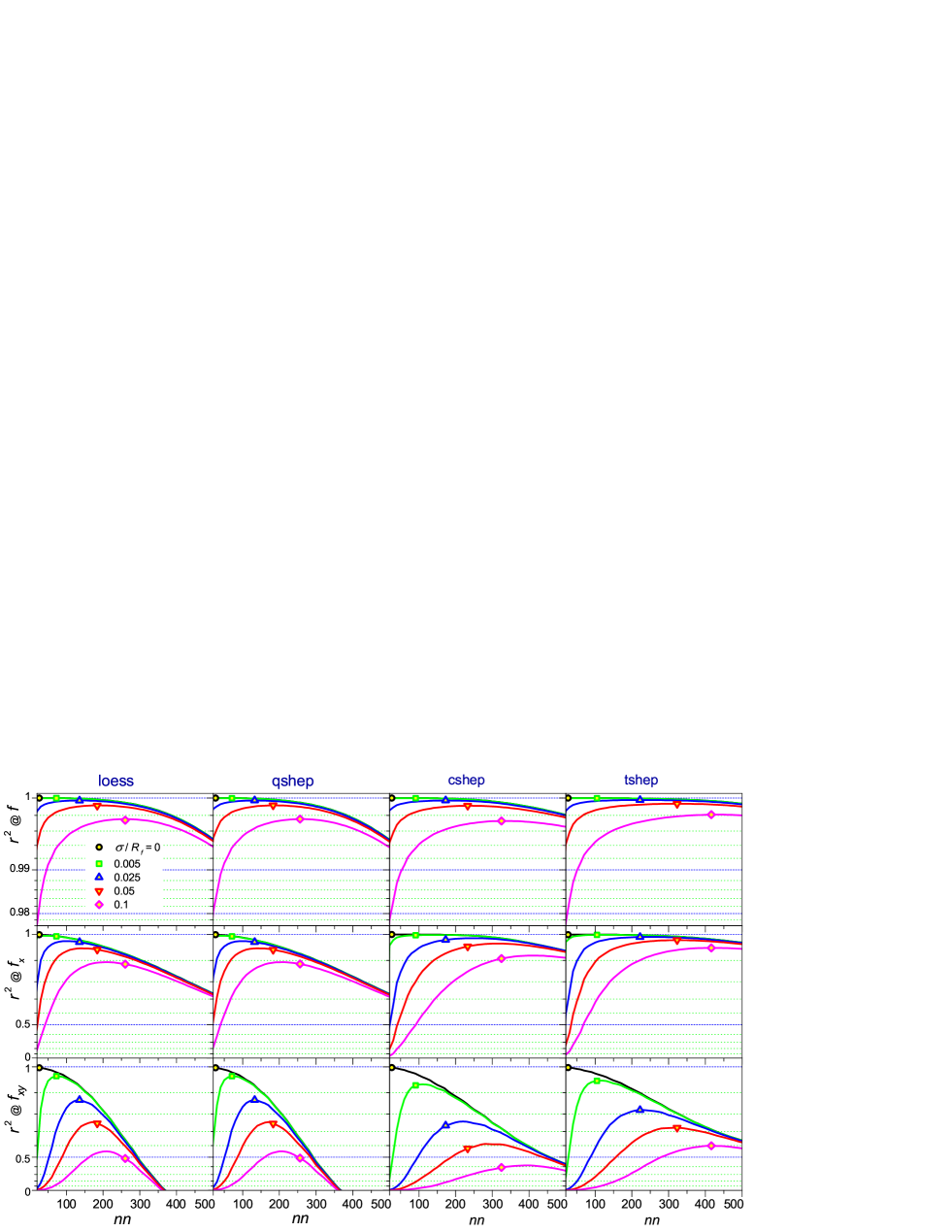
Figure 2: Dependence of the coefficient of determination $r^{2}$ on the on the number $nn$ of nearest neighbor data points used for the local nonparametric regression, for test function $f_{3}$ and for its first derivative $f_{x}$ and for the mixed derivative $f_{xy}$, for different amplitudes of the Gaussian noise. The symbols mark the values given by the automatic smoothing parameter selection with the $\mathrm{AIC_{C}}$ criterion.

Figure 3: FORC diagrams obtained with the loess method for $\sigma\left/R_{f}\right.=0.025$ and for different values of the smoothing parameter $nn$, along with the true diagram.

In order to study smoothing methods it is of paramount importance to use made-up data where the true model is known. Certainly in the usual application no representation of the true underlying function is known, but if a method approximates a variety of functions behavior faithfully, then we expect it to give reasonable results in other cases. Consequently, the implemented methods were tested for accuracy on artificial data sets constructed by adding Gaussian noise and/or outliers to different test functions.

Our test suite consists of 15 functions, some of them with multiple features and abrupt transitions. While all the test functions are continuous, some of them have a derivative discontinuity at one point, what make smoothing and the derivatives estimation quite challenging.supplementary material A dedicated GUI allows users to easily choose one of the functions, to add noise, outliers, and placement of the input points. Nodes placement can be varied from a regular grid to a complete spatial randomness. As doFORC is mainly dedicated to FORC diagrams calculation, the test functions $f_{3},f_{4},f_{5},$ and $f_{6}$ provide FORCs for different types of Preisach distributions. For all other functions the data can be generated either in a rectangular domain or in a FORC style in the $h_{\mathrm{applied}}\geq h_{\mathrm{reversal}}$ half-plane. The purpose is twofold: to guide users in the selection of an appropriate method and to provide a test suite for assessing the accuracy of other FORC type (or two dimensional smoothing) software tools that exist in the scientific literature.

In our tests one of the ways to characterize the error was taken to be $\mathrm{SSE}/\mathrm{SSM}$, where $\mathrm{SSE}=\sum\nolimits_{i=1}^{n}(\hat{f}_{i}-\mu_{i})^{2}$ is the sum of squared errors (deviations) from the true test function values, and $\mathrm{SSM}=\sum\nolimits_{i=1}^{n}(\hat{f}_{i}-\hat{f}_{\mathrm{mean}})^{2}$ is the sum of squares of deviations about the mean of the estimated values of dependent variable. This mean value is the “worst” regression model that always predicts the same value irrespective of the value of the independent variables. The coefficient of determination is defined as $r^{2}=1-\mathrm{SSE}/\mathrm{SSM}$. Basically $r^{2}=1$ implies no error in the estimated values, a “perfect” fit of the true data, while $r^{2}=0$ does not implies a total lack of fit, but rather an underfit (high bias) as will be noticed below. For brevity we will use the notations $h_{\mathrm{applied}},h_{\mathrm{reversal}},m$ or $x,y,f$ interchangeably.

We first present the results obtained using the test function $f_{3}$ with $\mu_{1}=3.7$, $\mu_{2}=0$, $\sigma_{1}=1$, $\sigma_{2}=2$, $\rho=0.2$ parameters on the $\left[-10,10\right]\times\left[-10,10\right]$ domain. The nodes placement was obtained starting from a $41\times 41$ regular grid by adding a uniform noise with the $0.1$ amplitude. To the true values of the regression function evaluated at input points $\left(x_{i},y_{i}\right)$ we have added a normal noise with mean $0$ and standard deviations $\sigma\left/R_{f}\right.=0.005,0.025,0.05,0.1$, where $R_{f}$ is the range of the test function over the given domain, the coefficient $r^{2}$ as well as the other quantities of interest being calculated as averages on 100 realizations of the input data (i.e., 100 different values of the seed that initialize the pseudorandom number generator). The same results were obtained by doubling the number of realizations. One of the realizations for each $\sigma\left/R_{f}\right.$ value is presented in Fig. 1, where we can observe that the input data with $\sigma\left/R_{f}\right.=0.1$ are quite noisy. Superimposed we present the corresponding smoothed (fitted) values in the input points, using the four regression procedures: loess, qshep (modified quadratic polynomial Shepard method), cshep (cubic polynomial), and tshep (cosine series), using automatic smoothing parameter selection with the $\mathrm{AIC}_{\mathrm{C}}$ criterion. We observe that the noise is greatly reduced by smoothing and the values estimated by the four methods almost overlap with the true values, differences being mainly obtained for the most noisy data, especially in the vicinity of the positive saturation, where the true FORCs almost coincide. These errors give rise to unreal negative zones in the FORC diagrams, close to the $h_{\mathrm{applied}}=h_{\mathrm{reversal}}$ diagonal (see Fig. 3).

In Fig. 2 we present the dependence of the coefficient of determination $r^{2}$ on the number $nn$ of nearest neighbor data points used for the local nonparametric regression, both for function and for the first derivative $f_{x}$ and for the mixed derivative $f_{xy}$, the results obtained for the other derivatives being similar. The symbols mark the values given by the automatic smoothing parameter selection with the $\mathrm{AIC}_{\mathrm{C}}$ criterion. The $\mathrm{AIC}_{\mathrm{C}_{1}}$ and GCV criteria provide proximate values (we note that the use of $\mathrm{AIC}_{\mathrm{C}_{1}}$ criterion with the loess method is not recommended for routine usage because computation time can be awful). Since in these tests with made-up data we know the real true values, we have computed both the Kullback-Leibler discrepancy between the smoothed estimate and the true function, as well the true average mean squared error MSE which characterizes the bias-variance tradeoff. All methods provide very close values for the selected “best” smoothing parameter $nn$.

One observes a remarkable agreement between the smoothing parameters $nn_{\mathrm{AICC}}$ that minimize the $\mathrm{AIC}_{\mathrm{C}}$ criterion and the maxima positions of the $r^{2}$ curves for the test function ($r^{2}@f$ ). We note that for this test function the $r^{2}@f$ curves have a rather flat maximum (and accordingly the curves $\mathrm{AIC}_{\mathrm{C}}$ have a flat minimum), which means that different values $nn$ around the maximum can have very similar performance on the smoothing performance. However, this is not an abnormal situation in regression, no diagnostic technique being able to provide an unequivocal answer, but rather a combination of diagnostic tools together with the visual analysis of both the fitted and original data can provide insight into the data. Hence, it is recommended to examine how the fit varies with since sometimes fits with different smoothing parameters can reveal features that can not be distinguished from just one “best” fit. Because both the loess and the qshep methods use quadratic polynomials for regression, and because the smoothed values are estimated in the input nodes, the results obtained using these two methods are very close (the difference between them being given by the different algorithms used for solving the least square equations). Instead, if the smoothed values would be evaluated at points different than the input nodes, then the loess method fit the values of $f$ on a set of nearby nodes, while the shep methods first build nodal (associated to the input nodes) functions that locally fits the data values and then the estimated smoothed value is defined as a convex combination of the nodal functions.

The $nn_{\mathrm{AICC}}$ also indicate well enough the maxima positions of the $r^{2}@f_{x}$ and $r^{2}@f_{xy}$ curves corresponding to the first and mixed derivatives $f_{x}$ and $f_{xy}$, respectively. This indicates that if the local regression fits well the data within the smoothing neighborhood, then the local slope provides a good approximation to the derivatives. Therefore the $\mathrm{AIC}_{\mathrm{C}}$ and GCV criteria can also be used for automatic smoothing parameter selection when the partial derivatives are to be estimated. As expected the value of $r^{2}$ decreases when estimating derivatives versus the function estimation, because differentiation increases the noise due to the propagation of errors.

We notice that in general as the complexity of the local approximant function increases the increases $r^{2}$ as well. Nevertheless, it must be taken into account that $r^{2}$ globally characterizes the goodness of fit, and that a more complex function can introduce oscillations into the approximate function and so a visual analysis of the estimated data is helpful.

In Fig. 2 we have represented the dependency of $r^{2}$ on $nn$ because users usually think in terms of smoothing parameter. However, in order to compare different amounts of smoothing being performed by different smoothing methods the smoothers should be placed on an equal footing. Using the same bandwidth does not give rise to comparable results as a higher order fit is more variable but less biased. Rather, number of degrees of freedom of a smoother is an indication of the amount of smoothing, and in Fig. 1ssupplementary material we present the dependency of on the degree of freedom DF1.

In Fig. 3 we present the FORC diagrams obtained with the loess method for $\sigma\left/R_{f}\right.=0.025$ and for different values of the smoothing parameter $nn$ along with the true diagram. Even if the input data are rather noisy the estimated diagrams capture the main features of the true diagram. The $nn=50$ determine an overfitted (high variance) result, while $nn=350$ (value for which $r^{2}@f_{xy}=0$) determine an underfitted (high bias) result.

In order to test the robustness of the four regression procedures to outliers we have added to $20\%$ of the input data a uniform noise with amplitude 10 times greater than that of the Gaussian noise. Fig. 2s from the supplementary materialsupplementary material shows that all methods are capable to provide useful results.

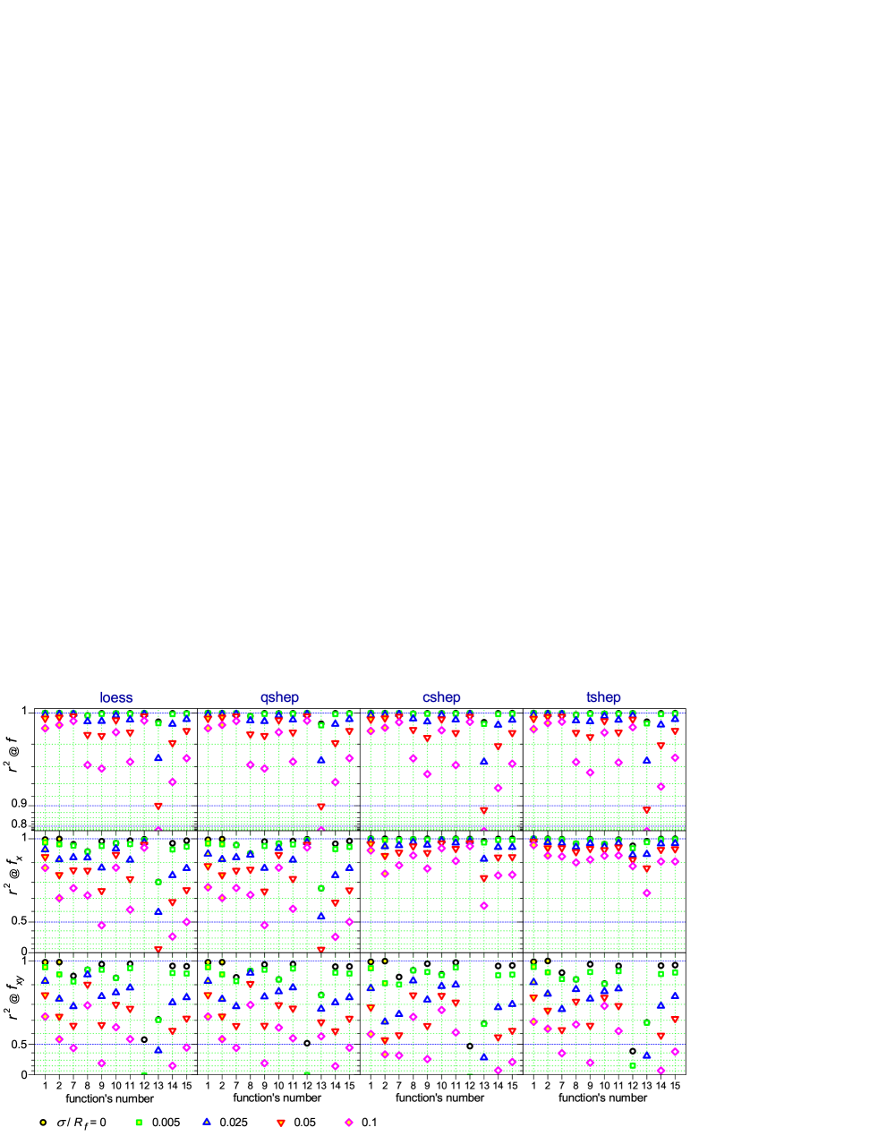
Figure 4: Coefficient of determination $r^{2}$ provided by the automatic smoothing parameter selection with the $\mathrm{AIC}_{\mathrm{C}}$ criterion for the test functions $f_{1},f_{2},f_{7},\ldots,f_{15}$.

Figure 4 summarizes some of the results of the tests performed using functions $f_{1},f_{2}$ with $\mu_{1}=$ $\mu_{2}=0$, $\sigma_{1}=2$, $\sigma_{2}=4$, $\rho=0.2$, and $f_{7},\ldots,f_{15}$ with $x_{c}=y_{c}=0$. The domain of the functions $f_{13},f_{14}$ was $\left[-1,1\right]\times\left[-1,1\right]$, of the function $f_{15}$ was $\left[-3,3\right]\times\left[-3,3\right]$, and for the other functions $\left[-10,10\right]\times\left[-10,10\right]$. For all functions we have used $41\times 41$ nodes randomly distributed throughout the corresponding rectangular domain. Functions $f_{10},f_{12},f_{13}$ have a first derivative discontinuity at the point $\left(0,0\right)$. As the function $f_{13}$ has a narrow spike maximum at $\left(0,0\right)$, covered only by 6 nodes in our test, its $r^{2}$ values are the smallest. We note that in fact local errors are large only near $\left(0,0\right)$, while in the other nodes the estimation is valuable. Although the function $f_{12}$ and its first derivative are well estimated by all regression methods, errors are high for the mixed derivative because the real derivative has very abrupt transitions.

It is noticed that in general the values of the first derivative are better estimated by the regression methods with higher complexity of the local approximant function.

XI Conclusions

We have presented the doFORC tool for calculating FORC diagrams of noise scattered data. The software is also able provide both a smooth approximation of the measured magnetization and all its partial derivatives. The implemented nonparametric regression methods were tested for accuracy on artificial data sets constructed by adding Gaussian noise and/or outliers to a set of 15 test functions, some of them with multiple features and abrupt transitions. Test performed by us have shown that all the implemented automatic smoothing parameter selection criteria provide reliable estimations of both smoothed magnetization and all its partial derivatives.

References

- (1) I. D. Mayergoyz, J. Appl. Phys. 57, 3803 (1985)
- (2) C. R. Pike, A. P. Roberts, and K. L. Verosub, J. Appl. Phys. 85, 6660 (1999).
- (3) A. Stancu, D. Ricinschi, L. Mitoseriu, P. Postolache, and M. Okuyama, Appl. Phys. Lett. 83, 3767 (2003).
- (4) A. P. Roberts, D. Heslop, X. Zhao, and C.R. Pike, Rev. Geophys. 52, 557 (2014).
- (5) F. Matau, V. Nica, P. Postolache, I. Ursachi, V. Cotiuga, and A. Stancu, J. Archaeol. Sci. 40, 914 (2013).
- (6) C. Enachescu, R. Tanasa, A. Stancu, E. Codjovi, J. Linares, and F. Varret, Physica B 343, 15 (2004).
- (7) R. Tanasa, C. Enachescu, A. Stancu, J. Linares, E. Codjovi, F. Varret, and J. Haasnoot, Phys. Rev. B 71, 014431 (2005).
- (8) C. Enachescu, R. Tanasa, A. Stancu, F. Varret, J. Linares, and E. Codjovi, Phys. Rev. B 72, 054413 (2005).
- (9) F. Preisach, Z. Phys. 94, 277 (1935).
- (10) H. G. Katzgraber, G. Friedman, G.T. Zimányi, Physica B 343, 10 (2004).
- (11) A. Stancu, C. Pike, L. Stoleriu, P. Postolache, and D. Cimpoesu, J. Appl. Phys. 93, 6620 (2003).
- (12) C. I. Dobrota and A. Stancu, J. Appl. Phys. 113, 043928 (2013).
- (13) M. Almasi-Kashi, A. Ramazani, and M. Amiri-Dooreh, Physica B 452, 124 (2014).
- (14) R. K. Dumas, P. K. Greene, D. A. Gilbert, L. Ye, C. Zha, J. Akerman, and K. Liu, Phys. Rev. B 90, 104410 (2014).
- (15) D. A. Gilbert, G. T. Zimányi, R. K. Dumas, M. Winklhofer, A. Gomez, N. Eibagi, J. L. Vicent, and K. Liu, Sci. Rep. 4, 4204 (2014).
- (16) M. Nica and A. Stancu, Physica B 475, 73 (2015).
- (17) D. Cimpoesu, I. Dumitru, and A. Stancu J. Appl. Phys. 120, 173902 (2016).
- (18) J. Gräfe, M. Weigand, N. Träger, G. Schütz, E. J. Goering, M. Skripnik, U. Nowak, F. Haering, P. Ziemann, and U. Wiedwald, Phys. Rev. B 93, 104421 (2016).
- (19) M. Rivas, J. C. Martínez-García, I. Škorvánek, J. Marcin, P. Švec, and P. Gorria, Appl. Phys. Lett. 107, 132403 (2015).
- (20) A. V. Ognev, K. S. Ermakov, A. Y. Samardak, A. G. Kozlov, E. V. Sukovatitsina, A. V. Davydenko, L. A. Chebotkevich, A. Stancu, and A. S. Samardak, Nanotechnology 28, 095708 (2017).
- (21) F. Beron, A. Kaidatzis, M. F. Velo, L. C. Arzuza, E. M. Palmero, R. P. Del Real, D. Niarchos, K. R. Pirota, and J. M. Garcia-Martin, Nanoscale Res. Lett. 11, 86 (2016).
- (22) A. Markou, K. G. Beltsios, L. N. Gergidis, I. Panagiotopoulos, T. Bakas, K. Ellinas, A. Tserepi, L. Stoleriu, R. Tanasa, and A. Stancu, J. Magn. Magn. Mater. 344, 224 (2013).
- (23) J. E. Davies, D. A. Gilbert, S. M. Mohseni, R. K. Dumas, J. Akerman, and K. Liu, Appl. Phys. Lett. 103, 022409 (2013).
- (24) F. Beron, M. A. Novak, M. G. F. Vaz, G. P. Guedes, M. Knobel, A. Caldeira, and K. R. Pirota, Appl. Phys. Lett. 103, 052407 (2013).
- (25) D. Heslop and A. R. Muxworthy, J. Magn. Magn. Mater. 288, 155 (2005).
- (26) D. Heslop and A. P. Roberts, Geochem. Geophys. Geosyst. 13, Q05016 (2012).
- (27) G. Acton, A. Roth, and K. L. Verosub, Eos, Transactions, American Geophysical Union 88, 230 (2007).
- (28) See http://paleomag.ucdavis.edu/software-forcit.html for the FORCit software package, which is a combination of Unix shell scripts, FORTRAN 77 subroutines, and Generic Mapping Tool (GMT) commands, all of which are available free of charge.
- (29) R. J. Harrison and J. M. Feinberg, Geochem. Geophys. Geosyst. 9, Q05016 (2008).
- (30) See http://wserv4.esc.cam.ac.uk/nanopaleomag/?page_id=31 and http://earthref.org/FORCinel for the FORCinel software package for the calculation of FORC diagrams. The FORCinel software is free, but runs inside Igor Pro by Wavemetrics (www.wavemetrics.com), which is a commercial software.
- (31) W. S. Cleveland, J. Am. Stat. Assoc. 74, 829 (1979).
- (32) W. S. Cleveland and S. J. Devlin, J. Am. Stat. Assoc. 83, 596 (1988).
- (33) W. S. Cleveland and E. Grosse, Stat. Comput. 1, 47 (1991).
- (34) C. Loader, Local Regression and Likelihood, Springer-Verlag New York Inc. (1999).
- (35) See www.netlib.org/a for the FORTRAN 77 implementation of the LOESS (LOcal regrESSion) method.
- (36) R. Egli, Global Planet. Change 110, 302 (2013).
- (37) See http://sites.google.com/site/irregularforc for the xFORC software package for the calculation of FORC diagrams. xFORC is freely available as an executable file which requires Labview run-time engine.
- (38) J. B. Abugri, P. B. Visscher, S. Gupta, P. J. Chen, and R. D. Shull, J. Appl. Phys. 124, 043901 (2018).
- (39) See http://stoner.phys.uaic.ro/doFORC for the doFORC software package for the calculation of FORC diagrams. The doFORC is a free, portable (standalone) application working on various operating systems.
- (40) D. Shepard, A two-dimensional interpolation function for irregularly-spaced data, Proceedings of the 1968 23rd ACM national conference, 517-524 (1968).
- (41) R. Franke and G. Nielson, Internat. J. Numer. Methods Engrg. 15, 1691 (1980).
- (42) R. J. Renka, ACM Trans. Math. Softw. 14, 139 (1988).
- (43) R. J. Renka, ACM Trans. Math. Softw. 25, 70 (1999).
- (44) R. J. Renka and R. Brown, ACM Trans. Math. Softw. 25, 74 (1999).
- (45) See www.netlib.org/toms/index.html for the FORTRAN 77 implementation of the modified Shepard methods.
- (46) See http://www.mps.mpg.de/dislin for the scientific data plotting software/library DISLIN (Device-Independent Software LINdau). DISLIN is free for non-commercial use.
- (47) P. Craven and G. Wahba, Numer. Math. 31, 377 (1979).
- (48) H. Akaike, Information theory and an extension of the maximum likelihood principle, Proceedings of the ”Second International Symposium on Information Theory, 1971”, Budapest Akademiai Kiado, pp. 267-281 (1973).
- (49) H. Akaike, IEEE T. Automat. Contr. 19, 716 (1974).
- (50) Akaike information criterion was developed by Hirotugu Akaike, originally under the name “An Information Criterion. ”It was first announced at a 1971 symposium, whose proceedings were published in 1973. The 1973 publication was only an informal presentation of the concepts, the formal publication being in 1974. In this paper is shown that “IC stands for information criterion and A is added so that similar statistics, BIC, DIC etc., may follow.”The 1974 paper is in the top 100 most cited research papers of all time according to Web of Science.
- (51) G. Schwarz, Ann. Stat. 6, 461 (1978).
- (52) S. Kullback and R. A. Leibler, Ann. Math. Stat. 22, 79 (1951).
- (53) C. M. Hurvich, J. S. Simonoff, and C. L. Tsai, J. R. Statist. Soc. B 60, 271 (1998).
- (54) T. J. Hastie and R. J. Tibshirani, Generalized Additive Models, New York: Chapman & Hall (1990).
- (55) See supplementary material at … for the kernel and test functions used by doFORC software, for a counterpart of Fig. 2 but as a function on the degree of freedom DF1, and for a counterpart of Fig. 2 but with outliers superimposed on the Gaussian noise.