Void distributions reveal structural link between jammed packings and protein cores

Abstract

Dense packing of hydrophobic residues in the cores of globular proteins determines their stability. Recently, we have shown that protein cores possess packing fraction $\phi\approx 0.56$, which is the same as dense, random packing of amino acid-shaped particles. In this article, we compare the structural properties of protein cores and jammed packings of amino acid-shaped particles in much greater depth by measuring their local and connected void regions. We find that the distributions of surface Voronoi cell volumes and local porosities obey similar statistics in both systems. We also measure the probability that accessible, connected void regions percolate as a function of the size of a spherical probe particle and show that both systems possess the same critical probe size. By measuring the critical exponent $\tau$ that characterizes the size distribution of connected void clusters at the onset of percolation, we show that void percolation in packings of amino acid-shaped particles and protein cores belong to the same universality class, which is different from that for void percolation in jammed sphere packings. We propose that the connected void regions of proteins are a defining feature of proteins and can be used to differentiate experimentally observed proteins from decoy structures that are generated using computational protein design software. This work emphasizes that jammed packings of amino acid-shaped particles can serve as structural and mechanical analogs of protein cores, and could therefore be useful in modeling the response of protein cores to cavity-expanding and -reducing mutations.

I Introduction

A significant driving force in protein folding is the sequestration of hydrophobic amino acids from solvent. Moreover, these buried amino acids are densely packed in the protein core (Dill, 1990). In fact, the packing of core residues has been linked directly to protein stability (Liang and Dill, 2001). For example, large-to-small amino acid mutations, which can increase interior protein cavities, or voids, are known to destabilize proteins when they are subjected to hydrostatic pressure (Roche et al., 2012; Nucci et al., 2014; Lerch et al., 2015) and chemical denaturants (Borgo and Havranek, 2012; Eriksson et al., 1992). Understanding the connection between dense core packing and voids is therefore crucial to understanding the physical origins of protein stability and reliably designing new protein structures that are stable (Sheffler and Baker, 2008). However, no such quantitative understanding yet exists, and it is currently difficult to distinguish computational protein designs that are not stable in experiments from experimentally observed structures (Fleishman and et. al., 2011).

In previous studies (Gaines et al., 2016, 2017a; Caballero et al., ), we found, using collective side chain repacking, that the side chain conformations of residues in protein cores (from a collection of high-resolution protein crystal structures) are uniquely specified by hard-sphere, steric interactions. Moreover, we have shown that, when considering hard-sphere optimized atomic radii, the core regions in proteins possess the same packing fraction $\phi\approx 0.56$ as that found in simulations of dense, random packings of purely repulsive, amino acid-shaped particles. This result suggests that the packing fraction of protein cores is determined by the bumpy and non-symmetric geometries of amino acids, and not on the backbone or local secondary structure.

However, materials that share the same packing fraction do not necessarily possess the same internal structure. In this article, we characterize the void space in experimentally obtained and computationally generated protein cores to further test the geometric similarities between these two systems. We show below that dense random packings of amino acid-shaped particles have the same local packing fraction, void distribution, and percolation of connected void space as protein cores, which indicates structural equivalence.

Our results suggest that the computationally generated packings can be used as mechanical analogs of protein cores to predict their collective mechanical response. Further, our results emphasize the connection between structurally arrested, yet thermally fluctuating, protein cores and the jamming transition of highly nonspherical particles (VanderWerf et al., 2018). Although the similarity between structural glasses and proteins at low temperatures has been known for several decades (Iben et al., 1989; Stein, 1985; Bryngelson and Wolynes, 1987; Loncharich and Brooks, 1990; Ringe and Petsko, 2003), prior computational studies have mainly focused on the transition from harmonic to anharmonic conformational fluctuations on length scales spanning the full protein. In contrast, our studies identify key structural similarities between jammed packings of amino acid shaped particles and the cores of protein crystal structures.

This article is organized into four sections and three appendices. In Sec. II, we describe the database of high-resolution protein crystal structures that we use for our structural analyses and the computational methods we use to generate jammed packings of amino acid-shaped particles. We also outline two methods to measure the void distribution in the two systems: a local measure of void space using surface Voronoi tessellation, and a non-local or “connected” measure of void space similar to that used by Kertèsz (Kertész, J., 1981) and Cuff and Martin (Cuff and Martin, 2004). In Sec. III, we compare the results of both the local and connected void measurements for jammed packings of amino acid-shaped particles and protein cores and find that both void measurements are the same for both systems. In Sec. III.1, we show that the Voronoi cell volume distributions in both systems are described by a $k$-gamma distribution with similar shape factors $k$. In addition, we find that the distribution of the local porosity ($\eta=1-\phi$) is the same for protein cores and jammed packings of amino acid-shaped particles. In Sec. III.2, we identify the percolation transition as a function of the probe particle accessibility for the connected voids, and find that protein cores and jammed packings of amino acid-shaped particles share the same critical probe size that separates the percolating and non-percolating regimes. We also investigate the critical properties of this percolation transition, and show that it is similar to void percolation of systems of randomly placed spheres, but different from void percolation in jammed sphere packings. In Sec. IV, we summarize our results, discuss their importance, and identify future research directions. We include three appendices with additional details of our computational methods. In Appendix A, we provide details for the computational method we use to generate jammed packings of amino acid-shaped particles. In Appendix B, we discuss the differences between protein cores in the Dunbrack 1.0 database, and the core replicas we generate from jammed packings of amino acid-shaped particles. In Appendix C, we discuss the differences between the connected void cluster size distributions in jammed packings of spheres and amino acid-shaped particles and systems containing randomly placed spheres.

II Methods

To benchmark our studies of local and connected void regions, we use a subset of the Dunbrack PISCES Protein Database (PDB) culling server (Wang and Dunbrack, 2003, 2005) of high-resolution protein crystal structures. This dataset, which we will refer to as “Dunbrack 1.0”, contains $221$ proteins with $<50\%$ sequence identity, resolution $\leq 1.0$ Å, side chain $B$ factors per residue $\leq 30$ Ų and $R$ factor $\leq 0.2$. We add hydrogen atoms to each protein crystal structure using the Reduce software (Word et al., 1999). To determine core amino acids, we calculate the solvent accessible surface area (SASA) for each residue using the Naccess software (Hubbard and Thornton, 1993) with a $1.4$ Å water molecule-sized probe (Gaines et al., ). To compare the SASA for residues with different sizes, we calculate the relative SASA (rSASA), which is the ratio of the SASA of the residue in the protein context to that of the residue outside the protein context, along with the C_α, C, and O atoms of the previous amino acid in the sequence and the N, H, and C_α atoms of the next amino acid in the sequence. We define core residues as those with rSASA $\leq 10^{-3}$. We find similar results if the threshold for defining a core residue is smaller, although there will be fewer “core” residues. We showed in previous work that the local packing fraction decreases significantly for residues with rSASA $>0.05$ (Gaines et al., ). (See Fig. 2 (a) for an example core region in a protein from the Dunbrack 1.0 database.)

Figure 1: Visualization of (a) local and (b) connected voids from the same computationally generated packing of $N=64$ amino acid-shaped particles. Only the central Alanine (Ala) with the neighboring Alanine, 2 Isoleucines (Ile), Leucine (Leu), and Valine (Val) are shown for clarity. The neighboring amino acids share at least one common surface Voronoi cell face with the central Ala. In (a), the central Ala is enclosed by its surface Voronoi cell. In (b), the connected void space is visualized using points on a grid. For clarity only $75\%$ of the points are shown, and the grid spacing $(g=0.7$Å) is large compared to values used in the text. In both (a) and (b), the atoms are colored as follows: C (green), O (red), N (blue), and H (white). See Fig. 8 for visualizations of the connected void space throughout the entire simulation domain.

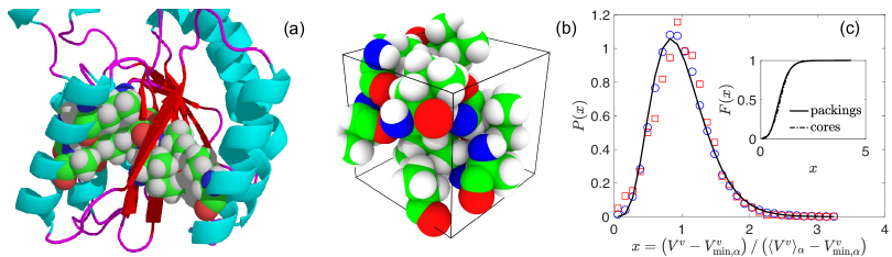
Figure 2: (a) Core residues in an example globular protein (PDB code: 3F1L). Non-core regions are drawn using the ribbon representation, and the $11$ core amino acids are drawn in all-atom representation. (b) Jammed packing of the same $11$ core residues in (a). (c) The surface Voronoi cell volume $V^{v}$ distribution plotted as a function of $x=(V^{v}-V^{v}_{\text{min},\alpha})/(\langle V^{v}\rangle_{\alpha}-V^{v}_{\text{min},\alpha})$ and fit to a $k$-gamma distribution (black line) with $k=6.06\pm 0.08$ and $5.29\pm 0.27$ for packings of amino acid-shaped particles (circles) and protein cores (squares), respectively. $\langle V^{v}\rangle_{\alpha}$ is the average and $V^{v}_{\min,\alpha}$ is the minimum SV cell volume of residue type $\alpha$. The inset of (c) is the cumulative distribution function $F(x)$ for the data in the main panel.

We will compare the structural properties of the cores of protein crystal structures and jammed packings (O’Hern et al., 2003) of amino acid-shaped particles. In previous studies, we found that the packing fraction of core regions in proteins is $\phi\approx 0.56$, which is the same as that of jammed packings of purely repulsive amino acid-shaped particles without backbone constraints (Gaines et al., 2016, 2017b). Here, we will focus exclusively on packing the hydrophobic residues: Ala, Leu, Ile, Met, Phe, and Val. The amino acid-shaped particles will include the backbone atoms N, C_α, C, and O, as well as all of the side chain atoms, with the atomic radii given in Ref. (Gaines et al., 2016), which recapitulate the side chain dihedral angles of residues in protein cores. The packings of amino acid-shaped particles contain mixtures of Ala, Leu, Ile, Met, Phe, and Val residues, with each residue treated as a purely repulsive, rigid body composed of a union of spherical atoms with fixed bond lengths, bond angles, and side-chain and backbone dihedral angles taken from instances in the Dunbrack 1.0 database.

We choose which residues are included in each packing using two methods. For method 1 (M1), we generate ${\cal C}=20$ jammed packings of the exact residues found in each distinct protein core in the Dunbrack 1.0 database. For example, if protein $X$ has a core with $R$ residues, we produce ${\cal C}$ jammed packings of those exact $R$ residues. If $r$ of these $R$ residues are not one of the hydrophobic residues we consider, these residues are removed and a jammed packing is generated with the remaining $R-r$ residues. This method seeks to mimic the core size and amino acid frequency distribution found in the Dunbrack 1.0 database. In method 2 (M2), we randomly select the hydrophobic residues with frequencies set by that for each hydrophobic amino acid found in protein cores in the Dunbrack 1.0 database. The frequencies are $0.29$ (Ala), $0.19$ (Leu), $0.17$ (Ile), $0.05$ (Met), $0.07$ (Phe) and $0.23$ (Val). In method 2, the identities of the residues in the jammed packings only match those in protein cores on average.

We now briefly describe the computational method for generating jammed packings of amino acid-shaped particles. We use a pairwise, purely repulsive linear spring potential to model inter-residue interactions. Because the residues are rigid particles with each composed of a union of spheres, we test for overlaps between residues $\mu$ and $\nu$ by checking for overlaps between all atoms $i$ on residue $\mu$ and all atoms $j$ on residue $\nu$, respectively. Note that this potential is isotropic and depends only on the distances between atoms on different residues. (See Eq. 14 in Appendix A.)

We place $N$ residues with random initial positions and orientations at packing fraction $\phi_{0}=0.40$ in a cubic simulation box with periodic boundary conditions and then increase the packing fraction in small steps $\Delta\phi$ to isotropically compress the system. After each compression step, we relax the total potential energy using FIRE energy minimization (Bitzek et al., 2006). This method is similar to a “fast” thermal quench that finds the nearest local potential energy minimum. We use quaternions to track the particle orientations for each residue, as described in Ref. (Rozmanov and Kusalik, 2010). If the total potential energy per residue is zero after energy minimization, i.e. $U/N\epsilon<10^{-8}$, where $\epsilon$ is the energy scale of the atomic interactions, we continue to increase the packing fraction. If the total potential energy per residue is nonzero, i.e. $U/N\epsilon\geq 10^{-8}$ and residues have small overlaps, we decrease the packing fraction. The packing fraction increment $\Delta\phi$ is halved each time the algorithm switches from compression to decompression and vice versa. We terminate the packing-generation protocol when the residue packings satisfy $10^{-8}<U/N\epsilon<2\times 10^{-8}$ and possess a vanishing kinetic energy per residue (i.e. $K/N\epsilon<10^{-20}$) (VanderWerf et al., 2018). (An example jammed packing of amino acid-shaped particles is shown in Fig. 2 (b) and further computational details are included in Appendix A.)

To measure the distribution of local voids in packings of amino acid-shaped particles and protein cores, we use Voronoi tessellation, which ascribes to each particle the region of space that is closer to that particle than all other particles in the system. For residues, which are highly non-spherical particles, we use a generalization of the standard Voronoi tessellation known as the surface- or set-Voronoi (SV) tessellation (M. Schaller et al., 2013). This tessellation partitions the empty space in the system using a bounding surface for each residue. An efficient algorithm to generate this tessellation is outlined in Ref. (M. Schaller et al., 2013) and implemented using Pomelo (Weis et al., 2017). To construct the SV tessellation, consider a set of $N$ particles with bounding surfaces $\quantity{\partial K_{\mu}}$ for $\mu=1,...,N$. The software approximates $\partial K_{\mu}$ by triangulating points on the particle surfaces, and uses standard Voronoi tessellation of the surface points to construct the SV cell for each residue $\mu$. We find that using $400$ surface points per atom, or $\approx 6400$ surface points per residue, gives an accurate representation of the SV cell, which does not change significantly as more surface points are added. An example SV cell from a packing of amino acid-shaped particles is shown in Fig. 1 (a). For an SV cell with volume $V^{v}_{\mu}$ surrounding residue $\mu$ with volume $v_{\mu}$, the local porosity is given by:

$$\eta_{\mu}=\frac{V^{v}_{\mu}-v_{\mu}}{V^{v}_{\mu}}=1-\phi_{\mu},$$ (1)

where $\phi_{\mu}=v_{\mu}/V^{v}_{\mu}$ is the local packing fraction. This quantity measures the local void space associated with each residue.

We also quantify the “connected” void space shared between residues in packings of amino acid-shaped particles and protein cores. To do this, we implement a grid-based method similar to that described by Kertèsz (Kertész, J., 1981) and Cuff and Martin (Cuff and Martin, 2004), where the “void space” is defined as the region of a system accessible to a spherical probe particle with radius $a$. The geometry and distribution of void space in a system is thus a function of $a$, the residue positions ${\vec{r}}_{\mu}$, and bounding surfaces $\partial K_{\mu}$. We define a cubic lattice with $G$ points in each direction within the simulation domain, which gives a lattice spacing $g=L/G$. For all lattice points $\mathbf{p}$, we define the set of void points $\mathcal{V}$ to be all points that can accommodate a spherical probe particle with radius $a$ without causing overlaps with any atoms. We label all void points with a $1$, and all other points with a $0$. After all grid points are labeled, we use the Newman-Ziff algorithm (Newman and Ziff, 2001) to cluster adjacent similarly labeled grid points. We consider all adjacent points on the nearest face, edge, and vertex of a cube of points surrounding each lattice point (i.e. next-to-next-to-nearest-neighbor counting with 26 possible adjacencies for each point) when merging void clusters and implement periodic boundary conditions. A sketch of connected void lattice points in a subset of a packing of amino acid-shaped particles is shown in Fig. 1 (b).

When measuring void space in protein structures, we implement a similar procedure, but we only consider voids in core residues. We construct a box of dimension $L_{x}\times L_{y}\times L_{z}$ that circumscribes each protein core, with the box just outside the radii of core residues near the box edges. We pick a spherical probe particle of radius $a$, and label the void space as all points that are (a) not contained inside an atom, and (b) contained only within the union of the SV cells of core residues. With these constraints, we only consider connected void space specific to the core of the protein. We then use the Newman-Ziff algorithm to merge void clusters, and repeat the procedure for 100 different random protein orientations.

III Results

III.1 Local Void Analysis

We begin with an analysis of local voids associated with each amino acid in jammed packings of amino acid-shaped particles and protein cores. We measure the distribution of the SV cell volumes and show that the distributions in both systems can be fit to a $k$-gamma distribution, which also describes Voronoi cell distributions in jammed packings of spheres (Aste and Di Matteo, 2008; Aste et al., 2007), ellipsoids (Schaller et al., 2016), attractive emulsion droplets Jorjadze et al. (2011), wet granular materials (Li et al., 2014), and model cell monolayers (Boromand et al., 2018). The $k$-gamma distribution for the SV cell volume $V^{v}_{\mu}$ for each residue has the form:

$$P(x)=\frac{k^{k}}{\Gamma(k)}x^{k-1}\exp(-kx),$$ (2)

where $x=\quantity(V^{v}_{\mu}-V^{v}_{\min,\alpha})/\quantity(\langle V^{v}_{\mu}\rangle_{\alpha}-V^{v}_{\min,\alpha})$, which sets the scale factor of the distribution to $1$. Here,

$$\langle V^{v}_{\mu}\rangle_{\alpha}=\frac{1}{N_{\alpha}}\sum_{\mu=1}^{N_{\alpha}}V^{v}_{\mu}$$ (3)

is the average SV cell volume of residue type $\alpha$. The sum involving $\mu$ is over all $N_{\alpha}$ residues of type $\alpha$ in all packings, and $V^{v}_{\min,\alpha}$ is the minimum SV cell volume of residue type $\alpha$. We consider minima and averages for each residue type separately to account for the large differences in residue volumes; that is, each residue type $\alpha$, when considered individually, has a SV cell volume distribution described by Eq. (2).

We measure the shape factor $k_{\alpha}$ for each residue type $\alpha$ either by fitting the SV cell volume distribution to Eq. (2) using Maximum Likelihood Estimation (MLE), or by calculating

$$k_{\alpha}=\frac{\quantity(\langle V^{v}_{\mu}\rangle_{\alpha}-V^{v}_{\min,\alpha})^{2}}{\left\langle\quantity(V^{v}_{\mu})^{2}\right\rangle_{\alpha}-\left\langle V^{v}_{\mu}\right\rangle_{\alpha}^{2}}.$$ (4)

We obtain similar $k$-values using both methods. Although the values of $k_{\alpha}$ depend on the type of amino acid $\alpha$, when we average the values of $k_{\alpha}$ we recover the value of $k$ obtained from fitting the combined distribution. We focus on the distributions of SV cell volumes averaged over all hydrophobic residues.

In Fig. 2 (c), we show the SV cell volume distributions $P(x)$ for packings of core amino acid-shaped particles modeled after specific protein cores (method M1) and for all core residues in the Dunbrack 1.0 database. We find that the distributions for these two systems are similar; both obey a $k$-gamma distribution [Eq. (2)] with similar shape parameters, $k=6.06\pm 0.08$ and $k=5.29\pm 0.27$, for core residues in the Dunbrack 1.0 database and packings of amino acid-shaped particles, respectively. As expected, the cumulative distributions $F(x)$ of the SV cell volumes for residues in protein cores and packings of amino acid-shaped particles are also nearly indistinguishable.

Figure 3: The shape parameter $k$ for fits of the $k$-gamma distribution [Eq. (2)] to the SV cell volume distributions $P(x)$ for packings of amino acid-shaped particles (open circles), monodisperse spheres (filled circles), and core residues in the Dunbrack 1.0 database (open squares) as a function of packing fraction $\phi$. The dashed horizontal line at $k=5.59$ is the analytical value of the shape factor for the Voronoi cell volume distribution of a random Poisson point process (Pineda et al., 2004), and the dashed vertical line at $\phi_{J}=0.56$ is the packing fraction for protein cores and jammed packings of amino acid-shaped particles.

Figure 4: Distribution of the scaled local porosity $y=(\eta-\eta_{\text{min},\alpha})/(\langle\eta\rangle_{\alpha}-\eta_{\text{min},\alpha})$, where $\langle\eta\rangle_{\alpha}$ is the average and $\eta_{\text{min},\alpha}$ is the minimum porosity of residue type $\alpha$, for packings of amino acid-shaped particles (circles) and residues in protein cores in the Dunbrack 1.0 database (squares). The solid line is a Weibull distribution with shape parameter $b\approx 3.2$ [Eq. (7)]. The inset is the cumulative distribution function $F(y)$ of the data in the main panel.

The strong similarity between the SV cell volume distributions indicates that jammed packings of amino acid-shaped particles (at $\phi_{J}\approx 0.56$) and protein cores possess the same underlying structure. To better understand this result, in Fig. 3 we plot the shape parameter $k$ that describes the form of the Voronoi cell volume distributions for packings of $N=10^{3}$ monodisperse spheres (with $\phi_{J}\approx 0.64$) and of $N=64$ amino acid-shaped particles versus $\phi$. When $\phi\ll\phi_{J}$, and the systems are sufficiently dilute, the Voronoi cell volume distributions of the packings of monodisperse spheres and amino acid-shaped particles resemble that for a random Poisson point process (Pineda et al., 2004) with $k\approx 5.6$. When $\phi\ll\phi_{J}$, free volume is assigned randomly to each particle since the particle positions are uncorrelated. However, as $\phi$ increases, the $k$-values for packings of monodisperse spheres and amino acid-shaped particles begin to grow, but at different rates, since the particle geometry becomes important in determining the local free volume. Near $\phi\simeq\phi_{J}$, the shape parameter plateaus at $k\approx 13$ for packings of monodisperse spheres, but the shape parameter decreases strongly to $k\approx 6$ for packings of amino acid-shaped particles. This decrease in $k$ indicates a transition from having the shape of the Voronoi cell volume distribution determined by independent, weakly correlated particles (for $\phi\lesssim\phi_{J})$ to having the shape of the distribution determined by bumpy, asymmetric amino acid-shaped particles (for $\phi\simeq\phi_{J}$).

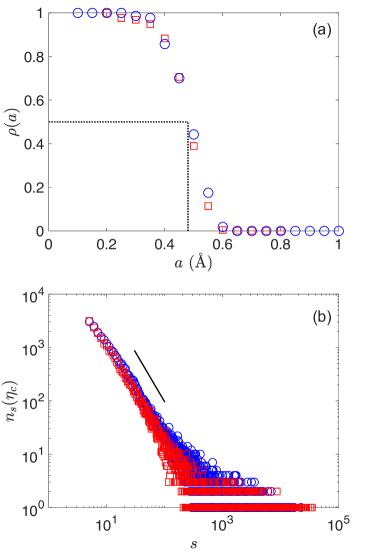
Figure 5: (a) Percolation probability $\rho(a)$ plotted versus the probe radius $a$ for protein cores from the Dunbrack 1.0 database (crosses) and clusters of core residues extracted from static packings of $N=64$ amino acid-shaped particles (circles). The horizontal and vertical dashed lines indicate the critical probe radius $a_{c}=0.48$ Å that satisfies $\rho(a_{c})=0.5$. (b) Number of connected void clusters $n_{s}$ with size $s$ at the percolating probe size $a_{c}$, which scales as $n_{s}(a_{c})\sim s^{-\tau}$. The Fisher power-law exponent $\tau=1.91\pm 0.1$ and $1.8\pm 0.09$ for protein cores from the Dunbrack 1.0 database (crosses) and representative clusters of core residues in packings of amino acid-shaped particles (circles), respectively. The solid line has slope equal to -1.85.

We also calculate $k$ for the SV cell volume distributions for core residues in the Dunbrack 1.0 database as a function of packing fraction. For most of the range in $\phi$, $k\approx 2$, whereas $k\gtrsim 5.6$ for packings of monodisperse spheres and amino acid-shaped particles. In particular, $k$ does not equal the value for a random Poisson point process ($k=5.6$) in the limit $\phi\ll\phi_{J}$ for residues in protein cores. In protein cores, the backbone constraint gives rise to correlations in the residue positions. However, as $\phi\to\phi_{J}$, $k$ increases, reaching $k\approx 6$ when $\phi=\phi_{J}$. This result shows that there is a fundamental change in the SV cell distribution near the onset of jamming in protein cores. For $\phi\lesssim\phi_{J}$, the backbone determines the shape of the Voronoi cell volume distribution, whereas for $\phi\to\phi_{J}$, the shapes of the amino acids determine the Voronoi cell volume distribution.

We also compare the local porosity distributions for protein cores and packings of amino acid-shaped particles in Fig. 4. We scale the porosity (as in Eq. (2)) by defining

$$y=\frac{\eta_{\mu}-\eta_{\min,\alpha}}{\langle\eta_{\mu}\rangle_{\alpha}-\eta_{\min,\alpha}},$$ (5)

where

$$\langle\eta_{\mu}\rangle_{\alpha}=\frac{1}{N_{\alpha}}\sum_{\mu=1}^{N_{\alpha}}\eta_{\mu},$$ (6)

and $\eta_{\min,\alpha}$ is the minimum porosity over all $N_{\alpha}$ core residues of type $\alpha$. Again, the porosity distributions $P(y)$ (and cumulative distributions $F(y)$) for residues in protein cores and packings of amino acid-shaped particles are similar, but here $P(y)$ has the shape of a Weibull distribution with scale factor $\lambda=1$,

$$P(y)=by^{b-1}\exp(-y^{b}).$$ (7)

where $b$ is the shape parameter of the Weibull distribution.

The small differences in $P(x)$ and $P(y)$ between core residues in protein crystal structures and packings of amino acid-shaped particles can be explained by the small differences between the volumes of core residues in crystal structures and in packings. The atoms on neighboring amino acids interact differently for free amino acids in packings versus backbone atoms in protein cores, which form covalent and hydrogen bonds. Thus, we find that the volumes of residues in protein cores have larger variances and smaller means than those in packings of amino acid-shaped particles. Also, the overlaps between covalently bonded backbone atoms that link adjacent residues slightly decreases the mean SV cell volume, which gives rise to a larger population of small SV cells and a small deviation between $P(x)$ for residues in protein cores and in packings for small $x$ in Fig. 2 (c).

III.2 Connected Void Analysis

Figure 6: Critical porosity $\langle\eta_{c}(G)\rangle$ using a lattice with $G$ points along each dimension plotted versus $G^{-1}$ for jammed packings of $N=10^{3}$ monodisperse spheres (filled circles) and of $N=64$ amino acid-shaped particles (open circles), and $N=10^{3}$ randomly placed spheres (open squares). The dashed lines have vertical intercepts that indicate $\eta_{c}\approx 0.0305$, $0.0318$, and $0.0343$ for the monodisperse sphere packings, packings of amino acid-shaped particles, and randomly placed spheres, respectively.

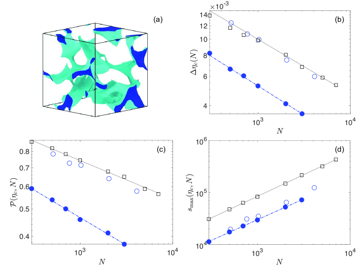
Figure 7: (a) Visualization of the surface of a connected void region (light domain) at the percolation threshold $\eta_{c}\approx 0.03$ in a jammed packing of $N=16$ amino acid-shaped particles (with $N_{a}=256$ atoms). The dark domains are the “inside” of the void region, which connects across the periodic boundaries. (b)-(d) Finite-size scaling behavior for jammed packings of amino acid-shaped particles (open circles), bidisperse spheres (filled circles), and randomly placed spheres (open squares). In (b), we show that the standard deviation in the critical porosity scales as $\Delta\eta_{c}(N)\sim N^{-1/d\nu}$, where $\nu$ is the correlation length exponent. The lines have slopes $-0.33$ (dotted line) and $-0.31$ (dot-dashed line). In (c), we show that the probability for a given site to be in the percolating void cluster at $\eta_{c}$ scales as ${\cal P}(\eta_{c},N)\sim N^{-\beta/d\nu}$, where $\beta$ is the percolation strength scaling exponent. The lines have slopes $-0.14$ (dotted line) and $-0.19$ (dot-dashed line). In (d), we show that the maximum cluster size near the percolation onset scales as $s_{\rm max}(\eta_{c},N)\sim N^{D/d}$, were $D$ is the fractal dimension. The lines have slopes $0.83$ (dotted line) and $0.82$ (dot-dashed line).

We next quantify the distribution of “connected” void space that is shared between residues. Using a grid-based method, we calculate the volume of regions of connected void space as a function of the radius $a$ of a spherical probe particle. As we increase $a$, the connected void space transitions from highly connected throughout the system to compact and localized with distinct void regions. We measure the probability $\rho(a)$ of finding a percolating void region, where we define percolation as the appearance of a cluster that spans one of the system dimensions when the boundary is closed, and a cluster that both spans, wraps around the boundary, and self-intersects when the boundaries are periodic. We identify the critical probe radius $a_{c}$ by setting $\rho(a_{c})=0.5$. Because the definition of connected void regions depends on the boundary condition, the value of $a_{c}$, especially in systems as small as protein cores, is affected by the boundary conditions. Thus, to calculate $\rho(a)$, we create packings of amino acid-shaped particles with similar boundary conditions as those in protein cores. From a packing of amino acid-shaped particles with periodic boundary conditions ($N=64$, method M2), we extract a representative protein core of $R-r$ residues that all share at least one SV cell face. We sample $R-r$ from the distribution of core sizes $P(R)$ found in the Dunbrack 1.0 database. (See Fig. 9 in Appendix A.) The resulting packings have boundary conditions similar to protein cores in the Dunbrack 1.0 database. We then determine the connected void regions as a function of $a$ and identify the critical probe size $a_{c}$ as shown in Fig. 5 (a). We find the same critical probe size $a_{c}=0.48\pm 0.01$ Å for both protein cores and packings of amino acid-shaped particles with similar boundary conditions. Note that this value of the critical probe radius is smaller than that of a water molecule, which is $\approx 1.4$ Å, and thus the voids we consider here are not accessible by aqueous solvents. However, as we discuss below, this value of the probe radius corresponds to a critical point; we will exploit the behavior of the voids near this critical point to understand the geometric properties of the connected voids, and to differentiate between the voids in various systems.

Thus, determining the connected void regions in protein cores is a type of percolation problem. In lattice site percolation, sites on a lattice in $d$ spatial dimensions are either occupied randomly with probability $p$ or not occupied with probability $1-p$. At the percolation threshold $p_{c}$, adjacent occupied sites form a percolating cluster that spans the system and becomes infinite in the large-system limit. Continuum percolation occurs in systems that are not confined to a lattice. Both particle contact and void percolation have been studied in randomly placed overlapping spheres (Kertész, J., 1981; Kerstein, 1983; Rintoul, 2000) and percolation of particle contacts (Rintoul and Torquato, 1997; Ostojic et al., 2006) has been studied in packings of repulsive (Shen et al., 2012) and adhesive particles (Lois et al., 2008).

In this article, we consider percolation of the void space accessible to a spherical probe particle with radius $a$ in packings of spheres and amino acid-shaped particles, as well as systems composed of randomly placed spheres (Kerstein, 1983; Rintoul, 2000). As the probe particle radius is increased, the amount of space available to the probe is restricted and the number of void lattice sites decreases. We define an effective porosity $\eta$ as the ratio of the number of void lattice sites to the total number of lattice sites $G^{d}$. We determine the percolation threshold using a bisection method, where we begin with two initial guesses for the percolation transition, $a_{H}$ and $a_{L}$ with $a_{H}>a_{L}$, and iteratively check for percolation of void sites at the probe radius $a=(a_{H}+a_{L})/2$. We set $a_{H}=a$ if we find a percolated cluster of void sites, and $a_{L}=a$ if we do not find a percolated cluster. We terminate the algorithm when the difference between successive values for $a_{c}$ are within a small tolerance $\delta a=10^{-8}$ Å. Note that our use of a lattice of points to measure the connected void region does not imply that our model is a lattice model. The lattice is simply a tool to calculate the connected void space volume (Kertész, J., 1981). Furthermore, in the continuum limit (i.e. $G\rightarrow\infty$), we recover the critical porosity $\eta_{c}\approx 0.03$ measured using Kerstein’s method (Kerstein, 1983; Rintoul, 2000) on systems of randomly placed spheres (Yi, 2006). (See Fig. 6.) Since there is a one-to-one mapping between $a$ and $\eta$, we will use $\eta$ as the order parameter for continuum void percolation.

We now focus on the statistical properties of the connected void regions in packings of spheres and amino acid-shaped particles. (See Fig. 7 (a) for an example connected void region in packings of amino acid-shaped particles.) We first measure the correlation length exponent $\nu$, where the correlation length $\xi$ is defined as the average distance between two points in the largest connected void cluster. Near $\eta_{c}$, $\xi$ diverges as $\absolutevalue{\eta-\eta_{c}}^{-\nu}$. Using finite-size scaling (Stauffer and Aharony, 1994), we can write

$$\eta_{c}(N)-\eta_{c}(\infty)\sim N^{-1/d\nu},$$ (8)

where $\eta_{c}(\infty)$ is the percolation threshold in the large-system limit and $N\sim L^{d}$. $\eta_{c}(N)$ is a random variable with standard deviation $\Delta\eta_{c}(N)$, which will approach $\eta_{c}(\infty)$ as $N\rightarrow\infty$. Thus, we make the ansatz that

$$\Delta\eta_{c}(N)\sim N^{-1/d\nu},$$ (9)

which can be used to measure $\nu$. (See Fig. 7 (b).) We also measure the probability ${\cal P}(\eta)$ that a given lattice site is part of the percolating void cluster. Near $\eta_{c}$, the probability scales as ${\cal P}(\eta)\sim\absolutevalue{\eta-\eta_{c}}^{\beta}$, where $\beta$ is the power-law exponent that characterizes the “percolation strength.” The probability obeys finite size scaling,

$${\cal P}(\eta,N)\sim N^{-\beta/d\nu}.$$ (10)

Once we determine $\nu$ using Eq. (9), we can determine $\beta$ from Eq. 10. (See Fig. 7 (c).) We also expect $\beta$ and $\nu$ to satisfy the hyperscaling relation,

$$D=d-\frac{\beta}{\nu},$$ (11)

where $D$ is the fractal dimension of the percolating void cluster. The fractal dimension is defined by

$$s_{\text{max}}(\eta_{c},N)\sim N^{D/d},$$ (12)

where $s_{\text{max}}(\eta_{c},N)$ is the number of sites contained in the largest void cluster in the system at percolation onset. If $D=d$, the largest void cluster is a compact, non-fractal object. However, if $D<d$, the void cluster is fractal (Grimmet, 1999). (See Fig. 7 (d).) We also measure the Fisher exponent $\tau$, defined by

$$n_{s}(\eta_{c})\sim s^{-\tau},$$ (13)

where $n_{s}$ is the number of void clusters containing $s$ sites. We measure this exponent for protein cores and random packings with representative boundary conditions in Fig. 5 (b).

System	$\nu$	$\tau$	$D$	$\beta$	$d-\frac{\beta}{\nu}$
residue packings (full)	$0.93\pm 0.02$	$1.15\pm 0.06$	$2.59\pm 0.09$	$0.40\pm 0.0089$	$2.57\pm 0.013$
residue packings (rep.)	$-$	$1.8\pm 0.08$	$-$	$-$	$-$
Protein cores, Dunbrack 1.0	$-$	$1.91\pm 0.09$	$-$	$-$	$-$
Mono. Spheres (jammed)	$1.07\pm 0.08$	$-$	$2.46\pm 0.04$	$0.60\pm 0.04$	$2.44\pm 0.06$
Bidis. Spheres (jammed)	$0.96\pm 0.01$	$-$	$2.40\pm 0.02$	$0.56\pm 02$	$2.41\pm 0.01$
Cubic Lattice	$0.91\pm 0.03$ ($0.88$)	$2.14\pm 0.05$ ($2.18^{\text{a}}$)	$2.49\pm 0.03$ ($2.53^{\text{a}}$)	$0.48\pm 0.02$ ($0.42^{\text{a}}$)	$2.48\pm 0.02$
Randomly Placed Spheres (connected void method)	$1.02\pm 0.04$	$1.1\pm 0.05$	$2.50\pm 0.02$	$0.42\pm 0.01$	$2.59\pm 0.02$
Randomly Placed Spheres (Voronoi vertex method)	$1.00\pm 0.05$ ($0.902\pm 0.005$)	$-$	$2.44\pm 0.02$	$0.5\pm 0.01$($0.45\pm 0.2$)	$2.50\pm 0.03$

Table 1: Table of critical exponents $\nu$, $\tau$, $D$, and $\beta$ for several models of void percolation. In the last column, we provide the value for the hyperscaling relation, $d-\frac{\beta}{\nu}$, which matches the fractal dimension $D$ if hyperscaling is satisfied. In the first four rows, we report the critical exponents for packings of amino acid-shaped particles with periodic boundary conditions (full) and boundary conditions representative of protein cores (rep.). We also report the critical exponents for void percolation in jammed packings of monondisperse (Mono.) and bidisperse (Bidis.) spheres. In the last four rows, we compare these results to those for void percolation in several systems that were studied previously. We report our measurements of the critical exponents for site percolation on a cubic lattice, where only nearest-neighbors are counted as adjacent sites. We also report the critical exponents for void percolation and Voronoi vertex percolation in systems composed of randomly placed spheres. Previously reported values of the exponents are given in parentheses.

In Table 1, we report our measurements for the critical exponents $\nu$, $\tau$, $D$, and $\beta$ for void percolation (using a spherical probe particle), as well as for $d=3$ lattice site percolation on a cubic lattice and void percolation in systems of randomly placed spheres using two methods: the connected void method described previously and the Voronoi vertex method introduced by Kerstein (Kerstein, 1983) and implemented by Rintoul (Rintoul, 2000). Note that protein cores and representative subsets of jammed packings of amino acid-shaped particles (denoted “rep.”) are small systems with $N<30$, and thus we cannot use finite-size scaling to measure the critical exponents. We can, however, measure the critical exponents for full packings of amino acid-shaped particles (denoted “full”), which mimic the geometric properties of void clusters in protein cores.

We observe that across all models and methods studied, the correlation length exponent $\nu\approx 0.9$-$1.0$ for void percolation. In particular, $\nu\approx 0.93$ for packings of amino acid-shaped particles is similar to that ($0.90$) for randomly placed spheres (Rintoul, 2000). In addition, the fractal dimension $D\approx 2.4$-$2.6$ is similar for all models and methods for calculating void percolation. We find that the percolation strength exponent $\beta<0.5$ for randomly placed spheres and packings of amino acid-shaped particles when using the connected void method, but $\beta>0.5$ for packings of monodisperse and bidisperse spheres. (The bidisperse systems include $N/2$ large and $N/2$ small spheres with diameter ratio $d=1.4$.) This result suggests that the geometry of connected void regions near percolation onset is most similar in packings of amino acid-shaped particles and systems of randomly placed spheres. In spite of the variations in the values of the exponents mentioned above, the hyperscaling relation [Eq. (11)] holds for most systems.

The Fisher exponent $\tau$ [Eq. (13)] provides even stronger evidence that the connected void regions in randomly placed spheres and packings of amino acid-shaped particles are similar near percolation onset. For these two systems, $\tau\approx 1.1$ and $1.15$. (See Table 1.) These values are distinct from those for protein cores and residue packings with boundary conditions similar to protein cores (i.e. $\tau\approx 1.8$ and $1.9$). $\tau$ is sensitive to boundary conditions, and thus we expect these $\tau$ values to differ. For lattice site percolation, $\tau\approx 2.14$ with periodic boundary conditions, which is distinct from $\tau$ measured in packings of amino acid-shaped particles and systems of randomly placed spheres with periodic boundary conditions.

We do not report values of $\tau$ for jammed packings of monodisperse and bidisperse spheres, since we observe non-power-law behavior in the cluster size distributions for these systems. As discussed in Appendix C, this behavior is most likely due to a residual finite length scale at the percolation threshold. We also observe non-power-law behavior in the cluster size distribution for void percolation in randomly placed spheres using Kerstein’s method, and do not report a value for $\tau$ in Table 1. However, as described in Appendix C, the non-power-law behavior is most likely due to system-size effects, which truncate the cluster size distribution. Thus, we conclude that the critical exponent $\tau$ is able to distinguish the geometries of connected void regions in different systems. Moreover, our results suggest that the connected void regions in packings of amino acid-shaped particles and systems of randomly placed spheres belong to the same universality class, which is distinct from that for jammed sphere packings. In Fig. 8, we show examples of the connected void surface in packings of (a) amino acid-shaped particles, (b) randomly placed spheres, and (c) bidisperse spheres. Qualitatively, the connected void surfaces in systems of randomly placed spheres and amino acid-shaped particles look similar, while the connected void surface in jammed packings of bidisperse spheres looks different, with a characteristic void size.

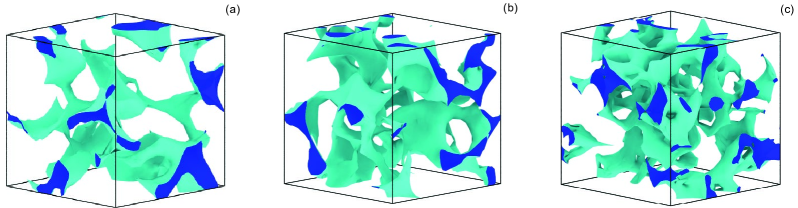
Figure 8: Visualization of the surface of connected void regions (light domains) near the percolation threshold in (a) a jammed packing of $N=300$ amino-acid shaped particles, (b) 300 randomly placed spheres, and (c) a jammed packing of $300$ bidisperse spheres. The darker domains indicate the inside of the void region, which connect across the periodic boundaries.

IV Conclusions and Future Directions

In this article, we analyzed local and connected void regions in protein cores and in jammed packings of purely repulsive amino acid-shaped particles and showed that these two systems share the same void structure. We first investigated the surface-Voronoi (SV) cell volume distributions and found that in both systems these distributions are well-described by a $k$-gamma distribution with $k\approx 6$. This $k$-value is much smaller than that ($k\approx 13$) obtained for jammed sphere packings, which indicates that packings of amino acid-shaped particles have a broader distribution of Voronoi volumes. We also studied the SV cell volume distribution as a function of the packing fraction, and found that only near the onset of jamming do the SV cell distributions in protein cores and packings of amino acid-shaped particles match. In the dilute case $\phi\ll\phi_{J}$, the local packing environment in protein cores is determined by the backbone, whereas the local packing environment of packings of free residues resembles a Poisson point process. At jamming onset, the local packing environment is determined by the “bumpy”, asymmetric shape of amino acids, not the backbone constraints.

Using a grid-based method, we also measured the distribution of non-local, connected voids in protein cores and jammed packings of amino acid-shaped particles. We found that when we consider similar boundary conditions in protein cores and jammed packings of amino acid-shaped particles, the two systems also have the same critical probe size $a_{c}$ (at which the accessible, connected void region spans the system) and Fisher exponent $\tau$ (which characterizes the scaling of the size of the void clusters near percolation onset). We also compare the finite-size scaling results for void percolation in packings of amino acid-shaped particles, in packings of monodisperse and bidisperse spheres, and systems of randomly placed spheres. We find that void percolation in packings of amino acid-shaped particles shares the same critical exponents as void percolation in randomly placed spheres. This result may also explain why the distribution of SV cell volumes is similar for jammed packings of amino acid-shaped particles and randomly placed spheres.

In future work, we will use jammed packings of amino acid-shaped particles to understand the structural and mechanical response of protein cores to amino acid mutations. We can assess the response in two ways. First, we can prepare jammed packings of amino acid-shaped particles that represent wildtype protein cores, substitute one or more of the wildtype residues with other hydrophobic residues, relax the “mutant” packing using potential energy minimization, and measure the changes in void structure. We can also measure the vibrational density of states (VDOS) in jammed packings that represent the wildtype and mutant cores. The VDOS and the associated eigenmodes can provide detailed information on how the low-energy collective motions change in response to mutations. There are several advantages for calculating the VDOS in jammed packings of amino acid-shaped particles. For example, in jammed packings, only hard-sphere-like steric interactions are included. In contrast, molecular dynamics force fields for proteins typically include many terms in addition to those that enforce protein stereochemistry, which makes it difficult to determine the interactions that control the collective motions. Studying jammed packings of amino acid-shaped particles also decouples the motions of core versus surface residues.

Studies of the VDOS in jammed packings of amino acid-shaped particles will also shed light on the protein “glass” transition, where the root-mean-square (rms) deviations in the atomic positions switch from harmonic to anharmonic behavior (Loncharich and Brooks, 1990) in globular proteins near $T_{g}\approx 200$ K (Ringe and Petsko, 2003). We will investigate the vibrational response of jammed packings of amino acid-shaped particles to thermal fluctuations. In particular, we will measure the Fourier transform of the position fluctuations and determine the onset of anharmonic response.

In addition, our analysis of void distributions in protein cores will provide new methods for identifying protein decoys, which are computationally generated protein structures that are not observed experimentally. However, it is currently difficult to distinguish between real structures and decoys. For example, in the most recent Critical Assessment of Protein Structure Prediction (CASP12), researchers were given a set of target sequences, and were tasked with predicting the structures of those sequences using a variety of methods (Moult et al., 2018). Each group was allowed to submit 5 structures per target sequence; when tasked with assessing which of their submissions were the most accurate, only 3 groups out of 31 had $>50\%$ success at identifying the most accurate structure (Hovan et al., 2018). The average success rate was $30\%$, just slightly better than guessing at random. Thus, assessing the viability of computationally-designed structures is an incredibly difficult task.

Since the structure of void regions in the cores of protein crystal structures is the same as that found in packings of amino acid-shaped particles, the properties of void regions can serve as a benchmark for ranking computationally designed protein structures. Recent studies have suggested that protein decoys (Sheffler and Baker, 2008) possess local packing fraction inhomogeneities that are not present in protein crystal structures. We propose that detailed characterizations of the void space, using the methods described here, will be a sensitive metric than can be used to assess a variety of protein designs.

Appendix A Packing-generation Protocol

As described in Sec. II, we generate jammed packings of amino acid-shaped particles using successive small steps of isotropic compression or decompression with each step followed by potential energy minimization. Each residue was modeled as a rigid union of spheres with fixed bond lengths, bond angles, and dihedral angles. The purely respulsive forces between residues were obtained by considering small overlaps between atoms on different residues, and then applying these forces to the center-of-mass of each residue, which gives rise to translational and rotational motion. Forces between atoms $i$ and $j$ on distinct residues $\mu$ and $\nu$ were calculated using ${\vec{F}}_{ij}^{\mu\nu}=-{\vec{\nabla}}U\quantity(r^{\mu\nu}_{ij})$, with the pairwise, purely repulsive linear spring potential energy,

$$U\quantity(r^{\mu\nu}_{ij})=\frac{\epsilon}{2}\quantity(1-\frac{r^{\mu\nu}_{ij}}{\sigma^{\mu\nu}_{ij}})^{2}\Theta\quantity(1-\frac{r^{\mu\nu}_{ij}}{\sigma^{\mu\nu}_{ij}}).$$ (14)

In Eq. 14, $\epsilon$ is the characteristic energy scale of the repulsive interactions, $\sigma^{\mu\nu}_{ij}=(\sigma^{\mu}_{i}+\sigma^{\nu}_{j})/2$, $r^{\mu\nu}_{ij}=|{\vec{r}}^{\mu}_{j}-{\vec{r}}^{\nu}_{i}|$ is the separation between atoms $i$ and $j$ on distinct residues $\mu$ and $\nu$, and $\Theta$ is the Heaviside step function that sets the potential energy to zero when atoms $i$ and $j$ are not in contact. Note that this pair potential reduces to a hard-sphere-like interaction in the limit of small atomic overlaps (Gaines et al., 2017b). The total potential energy $U$ is given by

$$U=\sum_{\nu<\mu}\sum_{i,j}U\quantity(r^{\mu\nu}_{ij}).$$ (15)

We use the velocity-Verlet algorithm to integrate the translational equations of motion for each particle’s center of mass, and a quaternion-based variant of the velocity-Verlet method described in Ref. (Rozmanov and Kusalik, 2010) to integrate the rotational equations of motions for each residue.

Figure 9: Distribution of the number of core residues $P(R)$ in the Dunbrack 1.0 database, before (circles) and after (squares) pruning non-hydrophobic residues from the core replicas as described in Sec. III.2. The mean number of residues before pruning is $\langle R\rangle\approx 16$, and after pruning is $\langle R-r\rangle\approx 12$.

Figure 10: Void cluster size distribution at percolation onset $n_{s}(\eta_{c})$ for (top) packings of amino acid-shaped particles (filled circles) and randomly placed spheres (open squares) and (bottom) jammed packings of monodisperse (filled circles) and bidisperse spheres (open triangles). In both panels, we use the connected void method to measure $n_{s}(\eta_{c})$. The distributions in the top panel have well-defined power-law decay for $s<10^{4}$, $n_{s}(\eta_{c})\sim s^{-\tau}$ with exponent $\tau\approx 1.1$, whereas the distributions in the bottom panel are not strict power-laws over the same range of $s$. The plateau regions at large $s$ are due to finite-size effects.

Figure 11: Cluster size distribution at percolation $n_{s}(\eta_{c})$ versus $s/\langle s\rangle$, normalized such that each curve has unit area, for void percolation though randomly placed spheres using Kerstein’s method with $N=300$ (dots), $10^{3}$ (squares), and $10^{4}$ (open circles). We also show the normalized $n_{s}(\eta_{c})$ calculated using the connected void method for $N=7\times 10^{3}$ randomly placed sphere (filled diamonds).

To simulate isotropic compression, we scale all lengths in the system (except the box edges) at each iteration $m$ by the scale factor

$$\alpha=\quantity(\frac{\phi_{m}+\Delta\phi_{m}}{\phi_{m}})^{1/3},$$ (16)

where $\phi_{m}$ is the packing fraction and $\Delta\phi_{m}$ is the packing fraction increment at iteration $m$. This process uniformly grows or shrinks all atoms, and thus the packing fraction satisfies $\phi_{m+1}=\phi_{m}+\Delta\phi_{m}$. After each compression or decompression step, we use the FIRE algorithm (Bitzek et al., 2006) to minimize the potential energy in the packing. The packing fraction increment is halved each time the total poential energy switches from zero (i.e. $U/N\epsilon<10^{-8}$) to nonzero or vice versa. We terminate the packing-generation algorithm when the total potential energy per residue satisfies $10^{-8}<U/N\epsilon<2\times 10^{-8}$ and the kinetic energy per residue is below a small threshold, $K/N\epsilon<10^{-20}$. We set the initial values of the packing fraction and packing fraction increment to be $\phi_{0}=0.4$ and $\Delta\phi_{0}=10^{-3}$, but our results do not depend sensitively on these values.

Appendix B Protein Core Size Distribution

In this Appendix, we show the distributions of the number of core residues in protein crystal structures from the Dunbrack 1.0 database. (See Fig. 9.) As described in Sec. II, we define protein cores as clusters of residues that all share at least one SV cell face with other residues in the cores, and every atom in each residue has an rSASA $\leq 10^{-3}$. In Method M1 for generating jammed packings of amino acid-shaped particles, we create ${\cal C}$ replicas of each protein core with the specific $R-r$ residues found in that core, where $R$ is the number of core residues and $R-r$ is the number of Ala, Ile, Leu, Met, Phe, and Val core residues. Before pruning non-hydrophobic residues, the average core size is $\langle R\rangle\approx 16$ residues, and $\langle R-r\rangle\approx 12$ after pruning.

Appendix C Measurement of the Fisher Exponent $\tau$

In this Appendix, we explain the differences we observe in the Fisher exponent $\tau$ for different systems. In systems of randomly placed spheres and in jammed packings of amino acid-shaped particles, the distribution of void cluster sizes at percolation onset $n_{s}(\eta_{c})$ has a well defined power-law decay, as shown in Fig. 10 (a). Non-power-law decay in the void cluster size distribution, as displayed in Fig. 10 (b) for jammed sphere packings, may be due to the existence of multiple important length scales in the system. The typical form of Eq. (13) at any porosity $\eta$ is (Stauffer and Aharony, 1994)

$$n_{s}=s^{-\tau}\exp(-s/s_{\xi}),$$ (17)

where $s_{\xi}$ is the number of sites in a cluster with correlation length $\xi$. In systems where $\xi$ is the only length scale, $s_{\xi}\rightarrow\infty$ as $\eta\rightarrow\eta_{c}$ and Eq. 17 reduces to Eq. (13). However, if there is another intrinsic length scale in the system that is still relevant at the void percolation transition, it is not necessarily true that $s_{\xi}\rightarrow\infty$. $s_{\xi}$ can remain finite, and add an exponential tail to $n_{s}(\eta_{c})$. Indeed, this behavior is what we find for the connected void size distribution in jammed sphere packings. The “kink” in $n_{s}(\eta_{c})$ in Fig. 10 (b) indicates that $s_{\xi}\approx 10$. .

This second length scale is most likely set by the neareast neighbor distances between particles. Qualitatively, if the nearest-neighbor distance between particles is a $\delta$-function (or a set of $\delta$-functions, in the case of polydisperse spheres), there are a limited number of local cavities in the system. In particular, there can be small, particle-scale voids that persist even even at the percolation threshold. However, in packings of amino acid-shaped particles and in systems of randomly placed spheres, there are a wide range of inter-particle distances, and a continuous range of local cavity sizes that can form. In Fig. 8, we show that the void regions are well-connected for jammed packings of amino acid-shaped particles and randomly placed spheres, while the void regions have a characteristic cavity size for jammed sphere packings at percolation onset. Thus, there is a well-defined Fisher exponent $\tau$ in jammed packings of amino acid-shaped particles and randomly placed spheres, but not in jammed monodisperse and bidisperse sphere packings.

References

- Dill (1990) K. A. Dill, Biochemistry 29, 7133 (1990).
- Liang and Dill (2001) J. Liang and K. A. Dill, Biophysical Journal 81, 751 (2001).
- Roche et al. (2012) J. Roche, J. A. Caro, D. R. Norberto, P. Barthe, C. Roumestand, J. L. Schlessman, A. E. Garcia, B. García-Moreno E., and C. A. Royer, Proceedings of the National Academy of Sciences 109, 6945 (2012).
- Nucci et al. (2014) N. V. Nucci, B. Fuglestad, E. A. Athanasoula, and A. J. Wand, Proceedings of the National Academy of Sciences 111, 13846 (2014).
- Lerch et al. (2015) M. T. Lerch, C. J. López, Z. Yang, M. J. Kreitman, J. Horwitz, and W. L. Hubbell, Proceedings of the National Academy of Sciences 112, E2437 (2015).
- Borgo and Havranek (2012) B. Borgo and J. J. Havranek, Proceedings of the National Academy of Sciences 109, 1494 (2012).
- Eriksson et al. (1992) A. E. Eriksson, W. A. Baase, X.-J. Zhang, D. W. Heinz, M. Blaber, E. P. Baldwin, and B. W. Matthews, Science 255, 178 (1992).
- Sheffler and Baker (2008) W. Sheffler and D. Baker, Protein Science 18, 229 (2008).
- Fleishman and et. al. (2011) S. J. Fleishman and et. al., Journal of Molecular Biology 414, 289 (2011).
- Gaines et al. (2016) J. C. Gaines, W. W. Smith, L. Regan, and C. S. O’Hern, Phys. Rev. E 93, 032415 (2016).
- Gaines et al. (2017a) J. Gaines, A. Virrueta, D. Buch, S. Fleishman, C. O’Hern, and L. Regan, Protein Engineering, Design and Selection 30, 387 (2017a).
- (12) D. Caballero, A. Virrueta, C. O’Hern, and L. Regan, Protein Engineering, Design and Selection , 367.
- VanderWerf et al. (2018) K. VanderWerf, W. Jin, M. D. Shattuck, and C. S. O’Hern, Phys. Rev. E 97, 012909 (2018).
- Iben et al. (1989) I. E. T. Iben, D. Braunstein, W. Doster, H. Frauenfelder, M. K. Hong, J. B. Johnson, S. Luck, P. Ormos, A. Schulte, P. J. Steinbach, A. H. Xie, and R. D. Young, Phys. Rev. Lett. 62, 1916 (1989).
- Stein (1985) D. L. Stein, Proceedings of the National Academy of Sciences 82, 3670 (1985).
- Bryngelson and Wolynes (1987) J. D. Bryngelson and P. G. Wolynes, Proceedings of the National Academy of Sciences 84, 7524 (1987).
- Loncharich and Brooks (1990) R. J. Loncharich and B. R. Brooks, Journal of Molecular Biology 215, 439 (1990).
- Ringe and Petsko (2003) D. Ringe and G. A. Petsko, Biophysical Chemistry 105, 667 (2003).
- Kertész, J. (1981) Kertész, J., J. Physique Lett. 42, 393 (1981).
- Cuff and Martin (2004) A. L. Cuff and A. C. R. Martin, Journal of Molecular Biology 344, 1199 (2004).
- Wang and Dunbrack (2003) G. Wang and R. L. Dunbrack, Jr., Bioinformatics 19, 1589 (2003).
- Wang and Dunbrack (2005) G. Wang and R. L. Dunbrack, Jr., Nucleic Acids Res 33, W94 (2005).
- Word et al. (1999) J. M. Word, S. C. Lovell, J. S. Richardson, and D. C. Richardson, Journal of Molecular Biology 285, 1735 (1999).
- Hubbard and Thornton (1993) S. J. Hubbard and J. M. Thornton, “Naccess,” (1993).
- (25) J. C. Gaines, S. Acebes, A. Virrueta, M. Butler, L. Regan, and C. S. O’Hern, Proteins 86, 581.
- O’Hern et al. (2003) C. S. O’Hern, L. E. Silbert, A. J. Liu, and S. R. Nagel, Phys. Rev. E 68, 011306 (2003).
- Gaines et al. (2017b) J. C. Gaines, A. H. Clark, L. Regan, and C. S. O’Hern, Journal of Physics: Condensed Matter 29, 293001 (2017b).
- Bitzek et al. (2006) E. Bitzek, P. Koskinen, F. Gähler, M. Moseler, and P. Gumbsch, Phys. Rev. Lett. 97, 170201 (2006).
- Rozmanov and Kusalik (2010) D. Rozmanov and P. G. Kusalik, Physical Review E 81, 056706 (2010).
- M. Schaller et al. (2013) F. M. Schaller, S. Kapfer, M. Evans, M. J. F. Hoffmann, T. Aste, M. Saadatfar, K. Mecke, G. W. Delaney, and G. Schröder-Turk, Philosophical Magazine 93 (2013).
- Weis et al. (2017) S. Weis, P. W. A. Schönhöfer, F. M. Schaller, M. Schröter, and G. E. Schröder-Turk, EPJ Web Conf. 140, 06007 (2017).
- Newman and Ziff (2001) M. E. J. Newman and R. M. Ziff, Phys. Rev. E 64, 016706 (2001).
- Aste and Di Matteo (2008) T. Aste and T. Di Matteo, Phys. Rev. E 77, 021309 (2008).
- Aste et al. (2007) T. Aste, T. D. Matteo, M. Saadatfar, T. J. Senden, M. Schröter, and H. L. Swinney, Europhysics Letters 79, 24003 (2007).
- Schaller et al. (2016) F. M. Schaller, R. F. B. Weigel, and S. C. Kapfer, Phys. Rev. X 6, 041032 (2016).
- Jorjadze et al. (2011) I. Jorjadze, L.-L. Pontani, K. A. Newhall, and J. Brujić, Proceedings of the National Academy of Sciences 108, 4286 (2011).
- Li et al. (2014) J. Li, Y. Cao, C. Xia, B. Kou, X. Xiao, K. Fezzaa, and Y. Wang, Nature Communications 5, 5014 EP (2014).
- Boromand et al. (2018) A. Boromand, A. Signoriello, F. Ye, C. S. O’Hern, and M. D. Shattuck, Preprint at https://arxiv.org/abs/1801.06150v3 (2018).
- Pineda et al. (2004) E. Pineda, P. Bruna, and D. Crespo, Phys. Rev. E 70, 066119 (2004).
- Kerstein (1983) A. R. Kerstein, Journal of Physics A: Mathematical and General 16, 3071 (1983).
- Rintoul (2000) M. D. Rintoul, Phys. Rev. E 62, 68 (2000).
- Rintoul and Torquato (1997) M. D. Rintoul and S. Torquato, Journal of Physics A: Mathematical and General 30, L585 (1997).
- Ostojic et al. (2006) S. Ostojic, E. Somfai, and B. Nienhuis, Nature 439, 828 EP (2006).
- Shen et al. (2012) T. Shen, C. S. O’Hern, and M. D. Shattuck, Phys. Rev. E 85, 011308 (2012).
- Lois et al. (2008) G. Lois, J. Blawzdziewicz, and C. S. O’Hern, Phys. Rev. Lett. 100, 028001 (2008).
- Yi (2006) Y. B. Yi, Phys. Rev. E 74, 031112 (2006).
- Stauffer and Aharony (1994) D. Stauffer and A. Aharony, Introduction to Percolation Theory (CRC Press, 1994).
- Grimmet (1999) G. Grimmet, Percolation, 2nd ed., Grundlehren der mathematischen Wissenschaften, Vol. 321 (Springer-Verlag Berlin Heidelberg, 1999).
- Moult et al. (2018) J. Moult, K. Fidelis, A. Kryshtafovych, T. Schwede, and A. Tramontano, Proteins: Structure, Function, and Bioinformatics 86, 7 (2018).
- Hovan et al. (2018) L. Hovan, V. Oleinikovas, H. Yalinca, A. Kryshtafovych, G. Saladino, and F. L. Gervasio, Proteins: Structure, Function, and Bioinformatics 86, 152 (2018).