¹¹institutetext: GEPI, Observatoire de Paris, Université PSL, CNRS, 61 Avenue de l’Observatoire, 75014 Paris, France
¹¹email: patrick.francois@obspm.fr ²²institutetext: Université de Picardie Jules Verne, 33 rue St Leu, Amiens, France ³³institutetext: GEPI, Observatoire de Paris, Université PSL, CNRS, Place Jules Janssen, 92190 Meudon, France ⁴⁴institutetext: Zentrum für Astronomie der Universität Heidelberg, Landessternwarte, Königstuhl 12, 69117, Heidelberg, Germany ⁵⁵institutetext: Max Planck Institute for Astronomy, Königstuhl 17, 69117, Heidelberg, Germany ⁶⁶institutetext: Zentrum für Astronomie der Universität Heidelberg, Institut für Theoretische Astrophysik, Albert-Ueberle-Strasse 2, 69120 Heidelberg, Germany ⁷⁷institutetext: Zentrum für Astronomie der Universität Heidelberg, Astronomisches Recheninstitut, Mönchhofstr. 12, 69120 Heidelberg, Germany ⁸⁸institutetext: Departamento de Ciencias Fisicas, Universidad Andres Bello, Fernandez Concha 700, Las Condes, Santiago, Chile ⁹⁹institutetext: Laboratoire Univers et Particules de Montpellier, LUPM, Université de Montpellier, CNRS, 34095, Montpellier cedex 5, France ¹⁰¹⁰institutetext: Leibniz-Institut für Astrophysik Potsdam (AIP), An der Sternwarte 16, 14482, Potsdam, Germany ¹¹¹¹institutetext: Istituto Nazionale di Astrofisica, Osservatorio Astronomico di Padova, Vicolo dell’Osservatorio 5, 35122, Padova, Italy

TOPoS

V: Abundance ratios in a sample of very metal-poor turn-off stars

P. François 1122 E. Caffau 33 P. Bonifacio 33 M. Spite 33 F. Spite 33 R. Cayrel 11 N. Christlieb 44 A. J. Gallagher 55 R. Klessen 66 A. Koch 77 H.-G. Ludwig 44 L. Monaco 88 B. Plez 99 M. Steffen 1010 S. Zaggia Based on observations collected at the European Organisation for Astronomical Research in the Southern Hemisphere under ESO programme ID 189.D-01651111

(Received ; accepted )

Abstract

Context. Extremely metal $-$ poor stars are keys to understand the early evolution of our Galaxy. The ESO large programme TOPoS has been tailored to analyse a new set of metal $-$ poor turn $-$ off stars, whereas most of the previously known extremely metal $-$ poor stars are giant stars.

Aims. Sixty five turn $-$ off stars (preselected from SDSS spectra) have been observed with the X $-$ Shooter spectrograph at the ESO VLT Unit Telescope 2, to derive accurate and detailed abundances of magnesium, silicon, calcium, iron, strontium and barium.

Methods. We analysed medium $-$ resolution spectra ( R $\simeq$ 10 000) obtained with the ESO X $-$ Shooter spectrograph and computed the abundances of several $\alpha$ and neutron $-$ capture elements using standard one $-$ dimensional local thermodynamic equilibrium (1D LTE) model atmospheres.

Results. Our results confirms the super-solar [Mg/Fe] and [Ca/Fe] ratios in metal $-$ poor turn $-$ off stars as observed in metal $-$ poor giant stars. We found a significant spread of the [ $\alpha$ /Fe] ratios with several stars showing sub $-$ solar [Ca/Fe] ratios. We could measure the abundance of strontium in 12 stars of the sample, leading to abundance ratios [Sr/Fe] around the Solar value. We detected barium in two stars of the sample. One of the stars (SDSS J114424 $-$ 004658) shows both very high [Ba/Fe] and [Sr/Fe] abundance ratios (¿ 1 dex).

Key Words.:

Galaxy - stars - abundances

1 Introduction

The study of the chemical composition of metal $-$ poor stars is one of the most important tools to understand and constrain the models for the early evolution of our Galaxy (see Beers & Christlieb, 2005; Frebel & Norris, 2015, and reference therein). In particular, detailed abundance ratios of the stars of the lowest [Fe/H] in our Galaxy contain information on the nature of the first stars which enriched the gas which subsequently formed the most metal $-$ poor stars we are observing. TOPoS (Turn $-$ Off PrimOrdial Stars) is a survey based on the ESO/VLT Large Programme 189.D-0165. The observation programme spanned four ESO semesters (Period 89 to period 92), from April 2012 to March 2014, for a total of 120 h with X-Shooter, and 30 h with UVES. The first paper of the series (Caffau et al., 2013a) contains the details of the TOPoS project. The main objectives of the survey are the following :

•

search for the extremely metal-poor (EMP) stars.
•

understand the formation of low $-$ mass stars in a metal $-$ poor environment.
•

use the detailed chemical composition of the most metal $-$ poor star to constrain the masses of the first Pop. III stars.
•

determine the Lithium abundance in these EMP stars.
•

derive the fraction the fraction of C $-$ enhanced EMP stars with respect normal EMP stars.

More details about these objectives can be found in Caffau et al. (2013a).

In the present paper, we focus on the determination of the chemical composition ( $\alpha$ and neutron $-$ capture elements) of the stars of the TOPoS sample. Eighty $-$ four metal $-$ poor candidates have been followed-up with X $-$ Shooter in total, and the most interesting stars, seven stars, have been followed $-$ up with UVES. The analysis of the UVES targets can be found in Bonifacio et al. (2018). The results concerning the first sample of 19 stars observed with X $-$ Shooter are presented in Caffau et al. (2013b). In this article, we report on the abundances of magnesium, silicon, calcium, strontium and barium for the remaining sample of 65 stars which have been observed with X $-$ Shooter.

2 Observations

The observations were performed in Service Mode with Kueyen (VLT $-$ UT2) and the high-efficiency spectrograph X $-$ Shooter (D’Odorico et al., 2006; Vernet et al., 2011). The X-Shooter spectra range from 300 nm to 2400 nm and are gathered by three detectors. The observations have been performed in staring mode with 1 $\times$ 1 binning and the integral field unit (IFU), which reimages an input field of 4.0 $\times$ 1.8″into a pseudo-slit of 12.0 $\times$ 0.6″(Guinouard et al., 2006). As no spatial information was available for our point $-$ source targets, we used the IFU as a slicer with three 0.6″slices. This corresponds to a resolving power of R = 7900 in the ultra $-$ violet arm (UVB) and R = 12 600 in the visible arm (VIS). Although the stellar light is divided into three arms by X $-$ Shooter (UVB, VIS and BIR), we only analysed the UVB and VIS spectra in this paper. The stars we observed are rather faint and have most of their detected flux in the blue and visible parts of the spectrum, so that the signal-to-noise ratio (S/N) of the infra-red spectra is too low to allow for any meaningful analysis to be conducted.

The spectra were reduced using the X $-$ Shooter pipeline (Goldoni et al., 2006), which performs the bias and background subtraction, cosmic ray $-$ hit removal (Van Dokkum, 2001), sky subtraction (Kelson, 2003), flat-fielding, order extraction, and merging. However, the spectra were not reduced using the IFU pipeline recipes. Each of the three slices of the spectra were instead reduced separately in slit mode with a manual localisation of the source and the sky. This method, which is not implemented in the current pipeline, allowed us to perform the best possible extraction of the spectra, leading to an efficient cleaning of the remaining cosmic ray hits, but also to a noticeable improvement in the S/N. Using the IFU can cause some problems with the sky subtraction, because there is only $\pm$ 1 $\arcsec$ on both sides of the object. In the case of a large gradient in the spectral flux (caused by emission lines), the modeling of the sky-background signal can be of poor quality owing to the small number of points used in the modeling. We experienced these difficulties for the NIR spectra and the reddest orders of the VIS spectra. For this analysis, the lines we measured were located in the wavelength range 390 - 650 nm.

3 Stellar parameters

The stellar parameters shown in Table LABEL:stellar_parameters have been computed following the method described in detail in Caffau et al. (2013a). Table LABEL:stellar_parameters includes the coordinates, the G magnitudes from Gaia DR2 (Gaia Collaboration al., 2016, 2018) and the SNR of the spectra. The effective temperature has been derived from the photometry, using the $(g-z)_{0}$ colour and the calibration described in Ludwig et al. (2008), taking into account the reddening according to the Schlegel et al. (1998) extinction maps and corrected using the techniques described in Bonifacio et al. (2000). As the stars of the sample were selected to have typical TO colours, an archetypical gravity of $\log g=4.0$ has been assumed for all stars. The micro-turbulent velocity has been set to 1.5 km/s. The determination of the [Fe/H] abundances was computed using the code MyGIsFOS (Sbordone et al., 2014). This code is based on the selection of clean Fe lines for which the equivalent width is measured ¹¹1 Equivalent widths of the Fe lines are only available at the CDS.. Further details about the determination of the [Fe/H] can be found in Caffau et al. (2013a). We do not report the radial velocities of the stars as it will be discussed in detail in a forthcoming paper.

4 Analysis

We carried out a classical 1D LTE analysis using MARCS model atmospheres (Gustafsson et al., 2008). The abundances used in the model atmospheres were solar-scaled with respect to the Grevesse & Sauval (2000) solar abundances, except for the $\alpha$ $-$ elements that are enhanced by 0.4 dex. We corrected the resulting abundances by taking into account the difference between Grevesse & Sauval (2000) and Caffau et al. (2011), Lodders et al. (2009) solar abundances. The final adopted solar abundances in this paper are: A(C)=8.50, A(Ca)=6.33, A(Mg)=7.54, A(Fe)=7.50, A(Si)=7.52, A(Sr)=2.92 and A(Ba)=2.17.

The abundance analysis was performed using the LTE spectral line analysis code turbospectrum (Alvarez & Plez, 1998; Plez, B., 2012), which includes continuum scattering in the source function (Cayrel et al., 2004). For each available transition, we computed a synthetic spectrum and compared the synthetic spectrum directly with the observed spectrum. We used the three lines of the magnesium triplet to derive the magnesium abundance. For silicon, we used the 390.5 nm line. The calcium abundance was measured using the lines at 422.6, 443.4 and 445.5 nm. We did not use the Ca II IR lines which is very likely caused by an incorrect sky subtraction. These lines are also known to be sensitive to departures from LTE, and are usually too strong for meaningful abundance determination. For strontium, we used the lines at 407.7 and 421.5 nm. Barium abundances were determined using the 455.4 nm line. We also evaluated the upper limits for the the carbon abundance by fitting the CH G $-$ band. Given that we selected our targets from spectra with weak CH G $-$ band, we do expect to find stars with a high carbon abundance. Indeed, we did not find any star with a high [C/Fe] ratio compatible with the high $-$ carbon band as defined by Spite et al. (2013). From our measurements, a fraction of the stars populates the low $-$ carbon band of the CEMP stars, but these upper limits are based on spectra with a rather low SNR and may give much higher carbon abundances than the true value. Indeed, the high [C/Fe] upper limits we measured are all found in the hottest stars of the sample, a temperature range for which the determination of the carbon abundance is particularly challenging. Further analyses with spectra of higher quality would help to give better estimates of the carbon abundance in these stars.

The abundances tabulated in Table LABEL:star_abund represent the best fit to the data. In some cases only a single transition has been measured providing a single abundance, whereas in others several lines have been measured and an average abundance is presented. The SNR of the reduced spectra presented in table LABEL:stellar_parameters may be used to evaluate the quality of the spectra. For the different elements studied in this article, we give the number of absorption lines that have been used to determine the abundances in Table LABEL:star_abund.

5 Errors

Table 1 lists the computed errors in the elemental abundances ratios due to typical uncertainties in the stellar parameters. The errors were estimated varying $T_{\mathrm{eff}}$ by $\pm$ 100 K, $\log\leavevmode\nobreak\ g$ by $\pm$ 0.3 dex and $v_{t}$ by $\pm$ 0.5 dex in the model atmosphere of SDSS J154746+242953, other stars give similar results. We chose this star because it has a temperature and ${\rm[Fe/H]}$ close to the median value of the ranges for the sample. Moreover, we could measure the Mg, Si, Ca, Ba and Sr abundances in this star. The main uncertainty comes from the error in the placement of the continuum when the synthetic line profiles are matched to the observed spectra. This error is of the order of 0.2 to 0.3 dex depending on the species under consideration. When several lines are available, the typical line $-$ to $-$ line scatter for a given elements is 0.1 to 0.2 dex.

6 Results and discussion

Table 1: Estimated errors in the element abundance ratios [X/Fe] for the star SDSS J154746+242953. The other stars give similar results.

[X/Fe]	$\Delta T_{\mathrm{eff}}$ =	$\Delta$ $\log\leavevmode\nobreak\ g$ =	$\Delta$ $v_{t}$ =
	100 K	0.3 dex	0.5 km/s
Mg	0.1	-0.1	-0.15
Ca	0.15	-0.1	0.15
Si	0.1	-0.1	-0.15
Sr	-0.2	0.2	0.25
Ba	0.2	0.2	-0.3

For most of the stars, we could derive the abundance of magnesium, silicon and calcium thanks to the strong lines of these species. We could also determine the abundance of strontium and barium for some of the targets. The results are gathered in Table LABEL:star_abund.

Refer to caption — Figure 1: Abundances in unevolved stars : the ratios [Mg/Fe] , [Si/Fe] and [Ca/Fe] for the program stars (red open circles) compared to those measured (grey and blue squares) by our group in other extremely metal-poor dwarf stars (Bonifacio et al., 2009, 2012, 2018; Caffau et al., 2013a, b). Blue (resp. grey) squares represent the stars which have been observed with UVES (resp. Xshooter). Pink squares represent dwarf stars analysed by Matsuno et al. (2017). Black dashed lines represent the linear fit to our data. Typical errors are represented in the lower left par of each panel.

6.1 Magnesium, calcium and silicon in turn $-$ off stars.

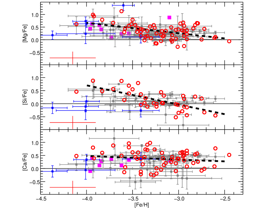
In Fig.1, we plot our results as red circles together with previous results from our group (Bonifacio et al., 2009, 2012, 2018; Caffau et al., 2013a, b). We add the results from Matsuno et al. (2017). It is important to note that this figure contains only turn $-$ off stars. The results we obtain for the new set of data seem to confirm previous results found for turn $-$ off stars, i.e. a slight increase of the [Mg/Fe] and [Si/Fe] abundance ratios at low [Fe/H], and a constant [Ca/Fe] abundance ratio, although with a larger scatter. The [Ca/Fe] ratios appear to be constant, on average, super-solar over the entire range of [Fe/H] values depicted. However, the results concerning dwarf stars analysed from UVES spectra by our group (blue symbols) seem to give lower abundance ratios. Below [Fe/H] $\simeq$ $-$ 4.0 dex, the abundance ratios found by previous studies seem to decrease down to values close to solar. This result should be taken with caution as it is based on few stars. If we consider the full set of results for turn $-$ off stars shown in Fig.1, the abundance ratios can be interpreted with a constant super-solar [Mg/Fe], [Si/Fe] and [Ca/Fe] ratios as found in giant stars (Cayrel et al., 2004), although with a larger scatter.

6.2 Abundance spread

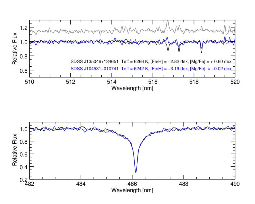
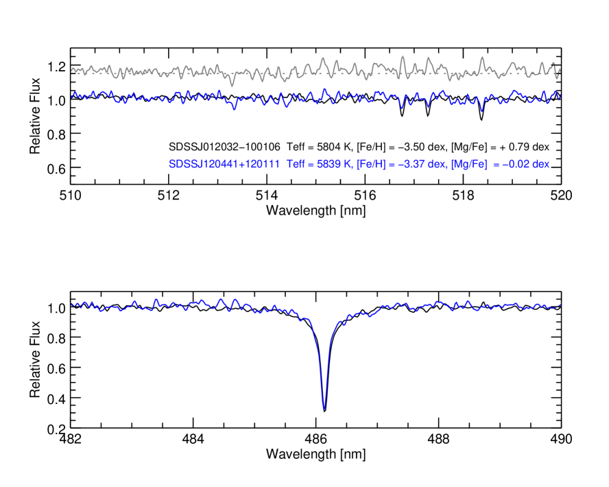
At a given metallicity, the [Mg/Fe] abundance ratios exhibit a significant scatter, which was already visible in the previous sample of TOPOS results represented as grey squares in Fig. 1. To verify the presence of the scatter, we identified ”twin stars” in our sample, i.e. stars with similar atmospheric parameters. We find two couples: the first pair SDSS J135046 $+$ 134651 and SDSS J104531 $-$ 010741 has an effective temperature of $\simeq$ 6200 K and [Fe/H] $\simeq$ $-$ 3.00 dex and the second pair SDSS J120441 $+$ 120111 and SDSSJ012032 $-$ 100106, with a $T_{\mathrm{eff}}$ $\simeq$ 5820 K and [Fe/H] $\simeq$ $-$ 3.45dex.

In Fig. 2 and Fig. 3, we plot the region where the magnesium triplet (top panel) and H $\beta$ (bottom panel) features form and over $-$ plotted the two sets of ”twin stars” over one-another. It is clear that neither ”twin star” share a similar magnesium abundance, based on the difference in their magnesium line strengths. The difference in the line strength of the Mg triplet line favours the existence of a real spread of the [Mg/Fe] ratio in stars with [Fe/H] $\lesssim$ $-$ 3.00 dex. The same conclusion can be drawn when inspecting the Ca and Si transitions in the same way in these two pairs of stars.

6.3 Temperature trends

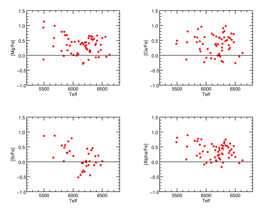
The abundance trends as a function of effective temperature in a sample of dwarf stars can be used to evaluate the presence of significant unknown absorption lines in the region of the transitions we studied. The strength of this unknown line would change as a function of temperature and would affect the derived abundance.

In Fig. 4, we show the ratios [Mg/Fe], [Ca/Fe], [Si/Fe] and the [ $\alpha$ /Fe] ratios (evaluated as 0.5 $\times$ ([Mg/Fe]+ [Ca/Fe]) as a function of the effective temperature of the star. We do not find any trend of the ratios [Mg/Fe], [Ca/Fe] and [ $\alpha$ /Fe] or their dispersion as a function of temperature; we measure a correlation coefficient of the order of 0.05 for the 3 sets of data. For Si, the results seem to indicate a variation of its abundance as a function of metallicity, an effect already found by Preston et al. (2006) . From their analysis based on high resolution high SNR spectra, they conclude that the silicon abundances measured in the cooler stars represent the true abundances of Si, hence an super-solar ratio. In the lower right panel of this figure, we present the mean abundance of magnesium and calcium, in order to minimize random errors. It is interesting to note a small decrease of the spread of the [ $\alpha$ /Fe] ratios at a given temperature compared to the [Mg/Fe] vs $T_{\mathrm{eff}}$ and [Ca/Fe] vs $T_{\mathrm{eff}}$ . However the spread is still present and is not correlated with temperature.

6.4 Strontium and barium

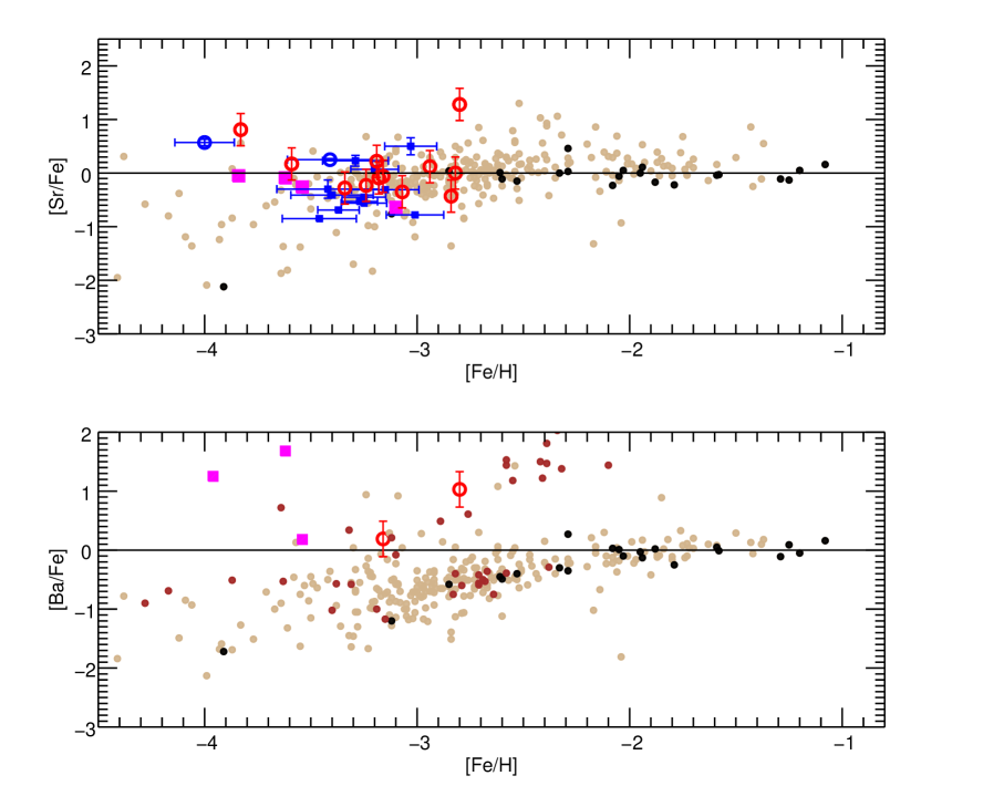
In Fig. 5, we plot our results for strontium and barium as red open circles together with the results from our group (Bonifacio et al., 2009, 2012, 2018; Caffau et al., 2013a, b). Blue symbols represent the metal-poor dwarf stars observed by our group (Bonifacio et al., 2009, 2012, 2018; Caffau et al., 2013a, b), the open blue circles denote stars which have been observed with UVES, whereas the blue squares are from X-Shooter spectra. We also add the results of Roederer et al. (2014) as light brown circles for evolved stars, and black circles for main $-$ sequence and turn $-$ off stars. The recent results of Matsuno et al. (2017) are represented as pink squares. Their sample has been selected from the Sloan Digital Sky Survey/Sloan Extension for Galactic Understanding and Exploration (SDSS/SEGUE), with follow-up observations with the Subaru telescope. In their paper, they selected eight unevolved stars with ${\rm T}_{\rm eff}\leq 5500\leavevmode\nobreak\ {\rm K}$ and ${\rm[Fe/H]}\leq$ - $3.5\leavevmode\nobreak\ {\rm dex}$ . They could measure the strontium abundance in four of them, and the barium abundance in three of them. The two most metal $-$ poor stars of their sample are suspected to be CEMP (carbon $-$ enhanced $-$ metal $-$ poor) s-stars, and can hence be considered as different from the stars of our sample, which does not contain any CEMP stars. For strontium, we report a good agreement with the results published in the literature for other turn $-$ off stars. The situation is more complex for barium. We find a systematic difference with the trend found by Roederer et al. (2014) for their sample of dwarf stars. However, this point has to be taken with caution as it is based on a very small sample. For the majority of the stars of our sample, we could not measure the barium abundance. Our results may simply reflect the limits of detection of the barium abundance in metal $-$ poor turn $-$ off stars from medium resolution and moderate SNR ratios.

The non CEMP s-star from the Matsuno et al. (2017) sample are above the solar [Ba/Fe] ratios as well. It is interesting to note that the sample of giant stars of Roederer et al. (2014) includes a significant number of stars with super-solar [Ba/Fe] ratios. Our stars seem to line up on this upper branch of stars, which have a rather high [Ba/Fe] ratio.

In order to investigate the nature of the stars found in this upper branch with super $-$ solar [Ba/Fe] ratios, we identified the CEMP stars (i.e. with [C/Fe] $>$ +1 dex) of the sample of Roederer et al. (2014) with brown circle symbols in the [Ba/Fe] vs [Fe/H] plot. The upper branch is mostly populated with CEMP evolved stars with a moderate [C/Fe] enhancement between 1 and 1.5 dex. Among them, the CEMP stars with [Fe/H] $>$ -2.6 dex are all CEMP $-$ s evolved stars leading to the conclusion that this upper branch reflects chemical characteristics from the population of CEMP stars, hence non related with the general galactic chemical evolution. However, there are several stars in this upper branch which are not CEMP $-$ s nor CEMP stars. This would be in favor of the existence of a real bimodal distribution. It is also interesting to note that none of main sequence stars of the sample of Roederer et al. (2014) belong to this upper branch. Further studies would be useful to refine the chemical diagnostic of these stars in this upper branch and evaluate the reality of a bimodal distribution.

The star SDSS J114424-004658 belonging to our sample shows both a high [Sr/Fe] and [Ba/Fe] ratio (larger than 1 dex). We also compute an upper limit of Europium for this star and found [Eu/Fe] $<$ 3.10 dex. This very high upper limit cannot be used to demonstrate that this star is a r $-$ process enriched star. High resolution, high SNR spectra would be necessary to derive the Europium abundance or at least a useful upper limit. This star is very similar to SDSSJ022226.20–031338.0 ([Fe/H]= $-$ 2.6 dex , [Ba/Fe] $\sim$ 2 dex , [Sr/Ba] $\sim$ 0.3 dex) studied by Caffau et al. (2018). As SDSS J114424-004658 is not too metal $-$ poor and not too faint (g=17.29), many neutron-capture absorption lines may be visible in high S/N high resolution spectra. This would be hence a very interesting target for follow-up observations.

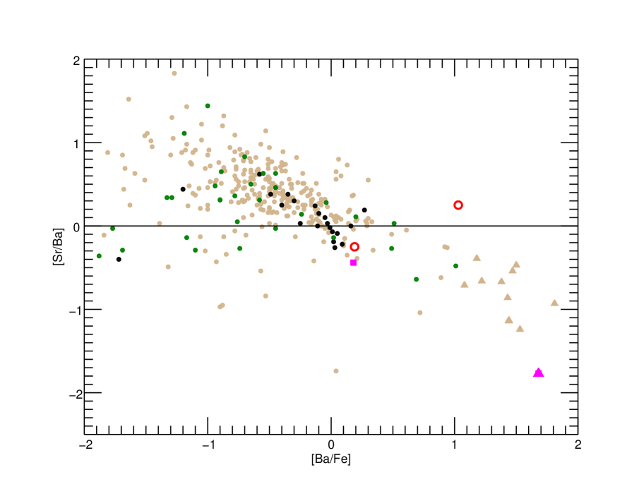
In Fig. 6, we plot the ratio [Sr/Ba] as a function of [Ba/Fe] for the two stars of our sample for which we could measure the abundances of these elements. We add the results of Roederer et al. (2014) as light brown circles black circles for main $-$ sequence and turn $-$ off stars. We also plot the results for Sr and Ba from the ESO large programme ”First Stars” (François & al., 2007).The two pink squares represent the results of Matsuno et al. (2017). The CEMP stars, which may to be considered as chemically peculiar stars, are represented as triangles. It is interesting to note the increase of the [Sr/Ba] ratio as [Ba/Fe] decreases, as mentioned for example by Spite et al. (2018) and François & al. (2007). Merging the results of Roederer et al. (2014) and Matsuno et al. (2017) shows that the decreasing (upper envelope) of the [Sr/Ba] abundance ratio as [Ba/Fe] increases seems to extend when [Ba/Fe] becomes super-solar. One of the stars for which we derived both Sr and Ba (SDSS J114424 $-$ 004658) does not follow this general trend. The star with [Ba/Fe] larger than 1 dex and negative [Sr/Ba] values in this plot is the CEMP-s star SDSS J1036+1212 (Matsuno et al., 2017), who confirmed the abundances found by Behara et al. (2010).

7 Conclusions

In the context of the TOPoS large programme, we have analysed sixty five metal $-$ poor turn $-$ off stars using X $-$ Shooter spectra increasing by more than a factor of two the number of metal-poor turn $-$ off stars with detailed abundances published in the literature. We measured the abundances of magnesium, calcium and silicon for most of the stars. We were able to derive the abundance of strontium in 12 stars and the abundance of barium in two stars of the sample. Both [Mg/Fe] and [Si/Fe] seem to show increasing relative abundance as [Fe/H] decreases down to [Fe/H] $\simeq$ $-$ 4.0 dex. However, in the metallicity interval $-$ 4 to $-$ 3 dex, there is a significant spread in [ $\alpha$ /Fe]. For strontium, we found from solar to slightly sub $-$ solar [Sr/Fe] ratios, in agreement with the results published in the literature. Two stars exhibits a high [Sr/Fe] (around +1 dex). The two stars for which we could measure the barium abundance show a super-solar ratio with one of them (SDSS J114424-004658) with a high [Ba/Fe] ratio of 1.28 dex. This star has a also a high [Sr/Fe] ratio and hence is an interesting target for follow $-$ up observations. This star is very similar to SDSSJ022226.20–031338.0 ([Fe/H]= $-$ 2.6 dex , [Ba/Fe] $\sim$ 2 dex , [Sr/Ba] $\sim$ 0.3 dex) studied by Caffau et al. (2018).These super-solar ratios are also found by Matsuno et al. (2017) in contrast with the results found by Roederer et al. (2014), who report a systematic sub-solar [Ba/Fe] ratio at the metal-poor end of their sample of turn-off stars. However, it is important to add that this effect is not found in their giants, for which they found both sub- and super-solar [Ba/Fe] ratios. Their results seem to indicate the presence of two distinct groups of stars in the metallicity range $-$ 3.2 dex $\leavevmode\nobreak\ \leq$ [Fe/H] $\leq$ $-$ 2.2 dex, one sample of stars with high [Ba/Fe] and a second sample with low [Ba/Fe]. However, a substantial fraction of the evolved stars found in this upper branch are CEMP $-$ s or CEMP stars. If further studies reveal that this is the case for all the stars in the upper branch, this would then reflect the peculiar chemical characteristics of this type of stars with no direct impact on the galactic chemical evolution.

It would be very interesting to study the barium abundance in turn-off stars in the metallicity range $-$ 3.2 dex $\leq$ [Fe/H] $\leq$ $-$ 2.2 dex to investigate the reality of a ”bimodal” distribution of the [Ba/Fe] ratios as a function of metallicity.

Acknowledgements.

PF, PB, EC, MS and FS acknowledge support from the Programme National de Physique Stellaire (PNPS) and the Programme National de Cosmologie et Galaxies (PNCG) of the Institut National des Sciences de l’Univers of the CNRS. AJG, NC, AK and HL were supported by Sonderforschungsbereich SFB 881 ”The Milky Way System” (subprojects A04, A05, A08) of the German Research Foundation (DFG). This work has made use of data from the European Space Agency (ESA) mission Gaia (https://www.cosmos.esa.int/gaia), processed by the Gaia Data Processing and Analysis Consortium (DPAC, https://www.cosmos.esa.int/web/gaia/dpac/consortium). Funding for the DPAC has been provided by national institutions, in particular the institutions participating in the Gaia Multilateral Agreement. We thank the anonymous referee for the very constructive report.

References

Alvarez & Plez (1998) Alvarez, R., & Plez, B. 1998, A&A, 330, 1109
Asplund et al. (1997) Asplund, M., Gustafsson, B., Kiselman, D., & Eriksson, K. 1997, A&A, 318, 521
Beers & Christlieb (2005) Beers, T. C.; Christlieb, N. 2005, ARA&A43, 531
Behara et al. (2010) Behara, N. T., Bonifacio, P., Ludwig, H.-G., Sbordone, L., González Hernández, J. I.; Caffau, E. 2010, A&A, 513, 72
Bonifacio et al. (2000) Bonifacio, P., Monai , Beers, T.C. 2000, AJ, 120,2065
Bonifacio et al. (2009) Bonifacio, P. et al. 2009, A&A 501, 519
Bonifacio et al. (2012) Bonifacio, P., Sbordone, L., Caffau, E. et al., 2012, A&A, 542, A87
Bonifacio et al. (2018) Bonifacio, P., Caffau, E., Spite, M. et al., 2018, A&A, 612, A65
Caffau et al. (2011) Caffau, E., Ludwig, H.-G., Steffen, M., Freytag, B., Bonifacio, P. 2011 Solar Phys 268, 255
Caffau et al. (2013a) Caffau, E.; Bonifacio, P.; François, et al. 2013a, A&A, 560, 15
Caffau et al. (2013b) Caffau, E.; Bonifacio, P.; Sbordone, L. et al. 2013b, A&A, 560, 71
Caffau et al. (2018) Caffau, E., Gallagher, A., Bonifacio, P. et al. 2018, A&A, 614, 68
Cayrel et al. (2004) Cayrel, R., Depagne, E., Spite, M. et al. 2004, A&A, 416, 1117
D’Odorico et al. (2006) D’Odorico, S., Dekker, H., Mazzoleni, R. et al. 2006 SPIE 6269, 33
François & al. (2007) François, P., Depagne, E., Hill, V. 2007, A&A, 476, 935
Frebel & Norris (2015) Frebel, A., Norris, J. 2015, ARA&A53, 631
Goldoni et al. (2006) Goldoni, P., Royer, F., Francois, P., Horrobin, M., Blanc, G., Vernet, J., Modigliani, A., Larsen, J. 2006 SPIE 6269, 2
Gaia Collaboration al. (2016) Gaia Collaboration and Prusti, T. et al. 2016 A&A595, 1
Gaia Collaboration al. (2018) Gaia Collaboration and Brown, A. G. A. et al. 2018 Summary of the contents and survey properties A&A616, A1
Grevesse & Sauval (2000) Grevesse, N. & Sauval, A. J. 2000, Origin of Elements in the Solar System, ed. O. Manuel, 261
Guinouard et al. (2006) Guinouard, I., Horville, D., Puech, M., Hammer, F., Amans, J-P, Chemla, F., Dekker, H., Mazzoleni, R. 2006 SPIE 6273, 3
Gustafsson et al. (2008) Gustafsson, Edvardsson, B., Eriksson, K., Jorgensen, U.G., Nordlund, A. , Plez., B. 2008, A&A, 488, 235
Kelson (2003) Kelson, D., 2003, PASP,115, 688
Lodders et al. (2009) Lodders, L., Palme, H., Gail, H-P, 2009, in Landolt-Börnstein, New Series, Astronomy and Astrophysics, Springer Verlag, Berlin
Ludwig et al. (2008) Ludwig, H.-G., Bonifacio, P., Caffau, E., Behara, N. T., Gonzalez Hernandez, J. I., Sbordone, L. 2008 Phys. Scr, 133
Matsuno et al. (2017) Matsuno, T., Aoki, W., Beers, T.C., Lee, Y.S., Honda, S. 2017 AJ, 154, 52
Plez, B. (2012) Plez, B., 2012, Turbospectrum : Code for spectral synthesis, Astrophysics Source Code Library, 1205.004
Preston et al. (2006) Preston, G.W., Sneden, C., Thompson, I.B., Shectman, S.A., Burley, G.S. 2006 AJ, 132, 85
Roederer et al. (2014) Roederer, I. U., Preston, G. W., Thompson, I. B.; Shectman, S. A., Sneden, C., Burley, G. S.; Kelson, D., 2014 AJ, 147, 136
Sbordone et al. (2014) Sbordone, L., Caffau, E., Bonifacio, P., Duffau, S., 2014, A&A564,109
Schlegel et al. (1998) Schlegel, D. J., Finkbeiner, D. P., Davis, M. 1998 ApJ, 500, 525
Spite et al. (2013) Spite, M., Caffau, E., Bonifacio, P. et al. 2013, A&A, 552, 107
Spite et al. (2018) Spite, F., Spite, M., Barbuy, B., Caffau, E., Bonifacio, P., François 2018, A&A, 611, 30
Van Dokkum (2001) Van Dokkum, P. 2001 PASP, 562, 35
Vernet et al. (2011) Vernet, J., Dekker, H., D’Odorico, S 2011 A&A, 536, 105

Appendix A Additional Tables

Table 2: Stellar parameters

STAR^a	$\rm T_{eff}$	[Fe/H]	$\alpha_{2000}^{b}$	$\delta_{2000}^{b}$	G^b	SNR@450 nm
SDSS J000411–055027	6174	–2.96	00:04:11.61	–05:50:28	19.0269	39
SDSS J002558–101509	6408	–3.08	00:25:58.60	–10:15:09	17.1013	52
SDSS J003507–005037	5891	–2.95	00:35:07.72	–00:50:38	17.3268	75
SDSS J003954–001856	6382	–2.94	00:39:54.66	–00:18:57	17.9868	63
SDSS J012032–100106	5804	–3.50	01:20:32.63	–10:01:07	16.3543	75
SDSS J012125–030943	6127	–2.91	01:21:25.11	–03:09:44	18.0162	36
SDSS J012442–002806	6273	–2.79	01:24:42.11	–00:28:07	18.9395	32
SDSS J014036+234458	5848	–3.83	01:40:36.22	+23:44:58	15.3520	69
SDSS J014721+021819	5967	–3.30	01:47:21.86	+02:18:20	17.0625	57
SDSS J014828+150221	6151	–3.41	01:48:29.01	+15:02:21	17.9115	66
SDSS J021238+013758	6291	–3.34	02:12:38.49	+01:37:58	17.2226	53
SDSS J021554+063901	6005	–2.75	02:15:54.33	+06:39:01	18.7562	37
SDSS J030549+050826	6309	–2.98	03:05:49.64	+05:08:27	18.9920	43
SDSS J031348+011456	6335	–3.31	03:13:48.15	+01:14:56	19.0425	38
SDSS J035925–063416	6281	–3.17	03:59:25.57	–06:34:16	18.0274	66
SDSS J040114–051259	5500	–3.62	04:01:14.73	–05:12:59	18.1712	33
SDSS J074748+264543	6434	–3.36	07:47:48.61	+26:45:43	17.0241	76
SDSS J075338+190855	6439	–2.45	07:53:38.62	+19:08:56	17.0073	38
SDSS J080336+053430	6360	–2.94	08:03:36.58	+05:34:30	16.7814	56
SDSS J082506+192753	6390	–3.07	08:25:06.66	+19:27:53	17.6095	69
SDSS J085232+112331	6206	–3.45	08:52:32.90	+11:23:31	18.0203	63
SDSS J090533–020843	5974	–3.44	09:05:33.36	–02:08:45	16.4991	54
SDSS J091913+232738	5490	–3.25	09:19:13.14	+23:27:38	18.3596	25
SDSS J103402+070116	6224	–3.58	10:34:02.70	+07:01:17	17.2439	57
SDSS J104531–010741	6242	–3.19	10:45:31.22	–01:07:42	19.0079	56
SDSS J105002+242109	5682	–3.93	10:50:02.36	+24:21:10	17.6611	57
SDSS J105231–004008	6199	–2.72	10:52:31.68	–00:40:09	18.2504	30
SDSS J112031–124638	6502	–3.27	11:20:31.81	–12:46:39	17.0484	56
SDSS J112211–114809	6157	–3.00	11:22:11.82	–11:48:09	18.5406	45
SDSS J112750–072711	6474	–3.34	11:27:50.90	–07:27:12	17.7014	81
SDSS J114424–004658	6412	–2.80	11:44:24.62	–00:46:59	17.0684	29
SDSS J120441+120111	5839	–3.37	12:04:41.39	+12:01:11	16.0913	44
SDSS J123055+000546	6223	–3.24	12:30:55.21	+00:05:47	14.4984	99
SDSS J123404+134411	5659	–3.59	12:34:04.57	+13:44:11	16.4659	54
SDSS J124121–021228	5672	–3.47	12:41:21.48	–02:12:29	18.9207	72
SDSS J124304–081230	5488	–3.92	12:43:04.16	–08:12:31	17.8240	53
SDSS J124719–034152	6332	–4.11	12:47:19.46	–03:41:52	18.2498	84
SDSS J131249+001315	6400	–2.38	13:12:49.61	+00:13:15	16.9237	34
SDSS J131456–113753	6265	–3.24	13:14:56.86	+11:37:53	17.4045	69
SDSS J131948+233436	6074	–2.61	13:19:48.62	+23:34:36	18.6605	32
SDSS J132112+010256	6395	–2.49	13:21:12.17	+01:02:56	18.9137	28
SDSS J132508+222424	6292	–2.60	13:25:08.60	+22:24:25	18.7498	28
SDSS J135046+134651	6266	–2.82	13:50:46.74	+13:46:51	18.0776	69
SDSS J135331–032930	6224	–3.18	13:53:31.00	–03:29:30	16.5132	83
SDSS J140007+191236	6570	–3.19	14:00:07.59	+19:12:36	19.0487	61
SDSS J141249+013206	5799	–2.94	14:12:49.07	+01:32:07	17.6992	30
SDSS J150702+005152	6555	–3.51	15:07:02.01	+00:51:53	18.5433	50
SDSS J153747+281404	6272	-3.39	15:37:47.78	+28:14:05	18.0039	54
SDSS J154746+242953	5903	-3.16	15:47:46.50	+24:29:53	17.8342	51
SDSS J155159+253900	6059	-3.08	15:51:59.34	+25:39:01	17.0147	35
SDSS J155751+190306	6176	-2.94	15:57:51.77	+19:03:06	17.5649	35
SDSS J172552+274116	6624	-2.91	17:25:52.21	+27:41:17	19.1727	33
SDSS J173358+274952	6088	-3.03	17:33:58.00	+27:49:52	18.9242	59
SDSS J200513-104503	6289	-3.41	20:05:13.50	-10:45:03	16.6015	55
SDSS J214633-003910	6475	-3.07	21:46:33.18	-00:39:10	17.8769	77
SDSS J215023+031928	6026	-2.84	21:50:23.52	+03:19:28	18.5872	34
SDSS J215805+091417	5942	-3.41	21:58:05.90	+09:14:17	18.0081	64
SDSS J220121+010055	6392	-3.03	22:01:21.77	+01:00:55	18.3999	66
SDSS J220728+055658	6096	-3.26	22:07:28.09	+05:56:59	18.1022	40
SDSS J222130+000617	5891	-3.14	22:21:30.23	+00:06:17	19.1787	33
SDSS J225429+062728	6169	-3.01	22:54:29.63	+06:27:28	18.4909	34
SDSS J230243-094346	5861	-3.71	23:02:43.34	-09:43:46	18.7481	56
SDSS J231031+031847	6229	-2.91	23:10:31.86	+03:18:48	16.7470	54
SDSS J231755+004537	5918	-3.54	23:17:55.56	+00:45:38	18.0750	56
SDSS J235210+140140	6313	-3.54	23:52:10.24	+14:01:40	17.9775	74
^a The name of the star is based on the SDSS DR12 coordinates.
^b From Gaia DR2.

Table 3: Abundance ratios [X/Fe] for the sample of stars. The number of lines used to compute the abundances of Mg, Si, Ca , Sr and Ba are given respectively in columns 5,7,9,11 and 13.

Object	[Fe/H]	[C/Fe]	[Mg/Fe]	n	[Si/Fe]	n	[Ca/Fe]	n	[Sr/Fe]	n	[Ba/Fe]	n
SDSS J000411 $-$ 055027	$-$ 2.96	¡ 1.20	0.37	3	$-$ 0.29	1	0.63	1	—-		—-
SDSS J002558 $-$ 101509	$-$ 3.08	¡ 1.52	0.49	3	—-		0.25	1	—-		—-
SDSS J003507 $-$ 005037	$-$ 2.95	¡ 0.69	0.68	4	0.30	1	0.47	3	—-		—-
SDSS J003954 $-$ 001856	$-$ 2.94	¡ 1.08	0.35	3	0.19	1	0.61	3	—-		—-
SDSS J012032 $-$ 100106	$-$ 3.50	¡ 0.94	0.79	3	0.55	1	0.62	2	—-		—-
SDSS J012125 $-$ 030943	$-$ 2.91	¡ 0.85	0.37	2	$-$ 0.44	1	0.68	1	—-		—-
SDSS J012442 $-$ 002806	$-$ 2.79	¡ 1.03	0.65	3	—-		0.26	1	—-		—-
SDSS J014036 $+$ 234458	$-$ 3.83	¡ 1.27	0.79	3	0.48	1	0.60	1	0.81	2	—-
SDSS J014721 $+$ 021819	$-$ 3.30	¡ 1.24	0.06	3	—-		$-$ 0.23	2	—-		—-
SDSS J014828 $+$ 150221	$-$ 3.41	¡ 0.95	0.42	3	$-$ 0.04	1	$-$ 0.12	1	—-		—-
SDSS J021238 $+$ 013758	$-$ 3.34	¡ 1.58	0.15	2	—–		0.91	2	—-		—-
SDSS J021554 $+$ 063901	$-$ 2.75	¡ 0.49	0.01	2	0.20	1	$-$ 0.08	2	—-		—-
SDSS J030549 $+$ 050826	$-$ 2.98	¡ 1.12	0.64	2	—-		0.60	2	—-		—-
SDSS J031348 $+$ 011456	$-$ 3.31	¡ 1.85	0.52	2	—-		0.98	1	—-		—-
SDSS J035925 $-$ 063416	$-$ 3.17	¡ 1.41	0.13	3	0.02	1	0.39	2	—-		—-
SDSS J040114 $-$ 051259	$-$ 3.62	¡ 0.86	1.13	3	0.87	1	0.49	2	—-		—-
SDSS J074748 $+$ 264543	$-$ 3.36	¡ 1.3	0.12	2	0.21	1	0.73	2	—-		—-
SDSS J075338 $+$ 190855	$-$ 2.45	¡ 1.39	-0.06	3	—-		0.52	1	—-		—-
SDSS J080336 $+$ 053430	$-$ 2.94	¡ 1.18	0.55	3	$-$ 0.11	1	0.51	2	0.12	2	—
SDSS J082506 $+$ 192753	$-$ 3.07	¡ 1.31	-0.07	3	—-		0.34	2	—-		—-
SDSS J085232 $+$ 112331	$-$ 3.45	¡ 1.39	0.31	3	—-		0.37	2	—-		—-
SDSS J090533 $-$ 020843	$-$ 3.44	¡ 1.78	0.45	3	0.79	1	0.61	2	—-		—-
SDSS J091913 $+$ 232738	$-$ 3.25	¡ 0.49	-0.14	3	—-		—-		—-		—-
SDSS J103402 $+$ 070116	$-$ 3.58	¡ 1.52	0.44	3	—–		0.05	2	—-		—-
SDSS J104531 $-$ 010741	$-$ 3.19	¡ 0.83	0.20	2	0.44	1	$-$ 0.04	2	0.22	2	—-
SDSS J105002 $+$ 242109	$-$ 3.93	¡ 1.17	1.29	3	0.88	1	0.00	2	—-		—-
SDSS J105231 $-$ 004008	$-$ 2.72	¡ 1.16	0.43	2	$-$ 0.33	1	$-$ 0.01	2	—-		—-
SDSS J112031 $-$ 124638	$-$ 3.27	¡ 1.71	0.58	3	0.02	1	$-$ 0.26	2	—-		—-
SDSS J112211 $-$ 114809	$-$ 3.00	¡ 0.94	0.41	3	$-$ 0.35	1	0.37	2	—-		—-
SDSS J112750 $-$ 072711	$-$ 3.34	¡ 1.88	0.35	3	$-$ 0.11	1	0.71	1	$-$ 0.28	1	—-
SDSS J114424 $-$ 004658	$-$ 2.80	¡ 1.54	0.66	3	—-		0.57	2	1.28	2	1.03	1
SDSS J120441 $+$ 120111	$-$ 3.37	¡ 0.81	-0.02	3	0.02	1	0.44	2	—-		—-
SDSS J123055 $+$ 000546	$-$ 3.24	¡ 1.08	0.25	3	$-$ 0.02	1	0.01	2	$-$ 0.23	2	—-
SDSS J123404 $+$ 134411	$-$ 3.59	¡ 0.63	0.30	3	0.14	1	—-		0.17	1	—-
SDSS J124121 $-$ 021228	$-$ 3.47	¡ 0.61	0.58	2	—-		0.44	2	—-		—-
SDSS J124304 $-$ 081230	$-$ 3.92	¡ 0.66	0.93	3	—-		0.39	2	—-		—-
SDSS J124719 $-$ 034152	$-$ 4.11	¡ 1.75	0.62	3	0.46	1	0.48	1	—-		—-
SDSS J131249 $+$ 001315	$-$ 2.38	¡ 1.52	—-		—-		—-		—-		—-
SDSS J131456 $-$ 113753	$-$ 3.24	¡ 1.38	-0.15	3	$-$ 0.11	1	$-$ 0.19	2	—-		—-
SDSS J131948 $+$ 233436	$-$ 2.61	¡ 0.85	0.07	3	—-		0.08	2	—-		—-
SDSS J132112 $+$ 010256	$-$ 2.49	¡ 1.73	—-		—-		—-		—-		—-
SDSS J132508 $+$ 222424	$-$ 2.60	¡ 1.24	0.11	3	$-$ 0.45	1	0.77	3	—-		—-
SDSS J135046 $+$ 134651	$-$ 2.82	¡ 1.06	0.58	3	0.27	1	0.54	3	0.00	2	—–
SDSS J135331 $-$ 032930	$-$ 3.18	¡ 1.12	0.34	3	0.03	1	0.60	1	$-$ 0.09	2	—–
SDSS J140007 $+$ 191236	$-$ 3.19	¡ 1.93	-0.05	2	—-		-0.04	2	—-		—-
SDSS J141249 $+$ 013206	$-$ 2.94	¡ 0.68	0.15	3	—-		0.66	1	—-		—-
SDSS J150702 $+$ 005152	$-$ 3.51	¡ 1.95	0.62	2	—-		—-		—-		—-
SDSS J153747 $+$ 281404	$-$ 3.39	¡ 1.83	0.40	3	—-		0.16	2	—-		—-
SDSS J154746 $+$ 242953	$-$ 3.16	¡ 0.90	0.17	3	0.31	1	0.13	2	$-$ 0.06	1	0.19	1
SDSS J155159 $+$ 253900	$-$ 3.08	¡ 1.02	-0.01	3	—-		—-		—-		—-
SDSS J155751 $+$ 190306	$-$ 2.94	¡ 1.08	-0.25	3	—-		0.31	2	—-		—-
SDSS J172552 $+$ 274116	$-$ 2.91	¡ 1.65	0.02	3	—-		0.08	2	—-		—-
SDSS J173358 $+$ 274952	$-$ 3.03	¡ 0.87	0.04	3	$-$ 0.52	1	$-$ 0.10	2	—-		—-
SDSS J200513 $-$ 104503	$-$ 3.41	¡ 1.65	0.17	3	—-		$-$ 0.22	2	—-		—-
SDSS J214633 $-$ 003910	$-$ 3.07	¡ 1.31	0.18	3	—-		0.44	3	$-$ 0.35	2	—-
SDSS J215023 $+$ 031928	$-$ 2.84	¡ 0.78	0.45	3	—-		0.21	2	$-$ 0.43	2	—-
SDSS J215805 $+$ 091417	$-$ 3.41	¡ 1.05	0.32	3	0.36	1	0.38	2	—-		—-
SDSS J220728 $+$ 055658	$-$ 3.26	¡ 1.50	0.47	3	—-		0.73	2	—-		—-
SDSS J220121 $+$ 010055	$-$ 3.03	¡ 1.27	0.39	3	-0.02	1	0.20	2	—-		—-
SDSS J222130 $+$ 000617	$-$ 3.14	¡ 1.28	0.35	3	—-		0.21	1	—-		—-
SDSS J225429 $+$ 062728	$-$ 3.01	¡ 1.25	-0.28	3	$-$ 0.04	1	0.38	2	—-		—-
SDSS J231031 $+$ 031847	$-$ 2.91	¡ 1.05	0.22	3	$-$ 0.14	1	0.58	2	—-		—-
SDSS J231755 $+$ 004537	$-$ 3.54	¡ 1.48	0.55	3	0.69	1	0.96	2	—-		—-
SDSS J230243 $-$ 094346	$-$ 3.71	¡ 1.15	0.67	3	0.56	1	0.88	2	—-		—-
SDSS J235210 $+$ 140140	$-$ 3.54	¡ 1.78	0.55	2	0.39	1	0.81	2	—-		—-