An easily-implemented, block-based fast marching method with superior sequential and parallel performance

Abstract

The fast marching method is well-known for its worst-case optimal computational complexity in solving the Eikonal equation, and has been employed in numerous scientific and engineering fields. However, it has barely benefited from fast-advancing multi-core and many-core architectures, due to the challenges presented by its apparent sequential nature. In this paper, we present a straightforward block-based approach for a highly scalable parallelization of the fast marching method on shard-memory computers. Central to our new algorithm is a simplified restarted narrow band strategy, with which the global bound for terminating the front marching is replaced by an incremental one, increasing by a given stride in each restart. It greatly reduces load imbalance among blocks through a synchronized exchanging step after the marching step. Furthermore, simple activation mechanisms are introduced to skip blocks not involved in either step. Thus the new algorithm mainly consists of two loops, each for performing one step on a group of blocks. Notably, it does not contain any data race conditions at all, ideal for a direct loop level parallelization using multiple threads. A systematic performance study is carried out for several point source problems with various speed functions on four grids with up to $1024^{3}$ points using two different computers. Substantial parallel speedups, e.g., up to 3–5 times the number of cores on a 16-core/32-thread computer and up to two orders of magnitude on a 64-core/256-thread computer, are demonstrated with all cases. As an extra bonus, our new algorithm also gives improved sequential performance in most scenarios. Detailed pseudo-codes are provided to illustrate the modification procedure from the single-block sequential algorithm to the multi-block one in a step-by-step manner.

35F30, 35L60, 49L25, 65N06, 65N22, 65K05

1 Introduction

The fast marching method [Sethian96, Sethian99a, Sethian99b] solves the stationary boundary value problem defined by the Eikonal equation:

(1) $$\begin{array}[]{cc}|\nabla\psi(\mathbf{x})|F(\mathbf{x})=1,&\mathbf{x}\in\varOmega\,\backslash\,\varGamma,\\ \psi(\mathbf{x})=0,&\mathbf{x}\in\varGamma\subset\varOmega,\end{array}$$

where $\varOmega$ is a domain in $\mathcal{R}^{n}$, $\varGamma$ is the initial boundary, and $F(\mathbf{x})$ is a positive speed function, with which the boundary information propagates away along characteristics in the domain. This equation has been used in a variety of applications, such as computational geometry, computer vision, optimal control, computational fluid dynamics, materials science, etc. The fast marching method is a non-iterative algorithm that closely resembles Dijkstra’s method [Dijkstra59] for finding the shortest path on a network. It was first proposed by Tsitsiklis [Tsitsiklis95] using an optimal control approach. Sethian [Sethian96] derived the algorithm based on an upwind difference scheme and introduced the name “fast marching”, which has since become a very popular method for solving the Eikonal equation.

The success of the fast marching method stems from its simplicity and efficiency. The discretization of the Eikonal equation using upwind difference schemes is straightforward. At a given grid point, the finite difference stencil contains only upwind neighbors and the causality of the equation is strictly followed. In terms of data structure, it only involves a heap priority queue, which is used to march the solution in a rigorous increasing order. In the fast marching method, the number of times that a point is visited is minimized and no iterations are involved in the one-pass solution updating process. For a case with $N$ grid points, the fast marching method has a worst-case optimal algorithm complexity of $O(N\log N)$, as the run-time complexity of reordering of a heap of length $n$ is $O(\log n)$.

Several studies have been reported to improve the $O(N\log N)$ run-time complexity to obtain $O(N)$ complexities for solving the Eikonal equation in a single pass. In particular, Tsitsiklis proposed a $O(N)$ approach using a bucket data structure along with his $O(N\log N)$ Dijkstra-like method [Tsitsiklis95]. Since insertion and deletion of a node in a bucket structure takes only $O(1)$ computations instead of $O(\log n)$ in the binary heap implementation of a priority queue, the complexity of the whole algorithm was reduced to $O(N)$. A shared-memory parallel implementation was also provided. In [YatzivBS06], an $O(N)$ implementation of the fast marching method was developed with the help of untidy priority queue that does not distinguish the priorities of the points within the same bucket. However, the quantization of the priorities introduces an extra error of the same order of magnitude of the discretization scheme. The $O(N)$ methods in [Tsitsiklis95] and [YatzivBS06] are single-pass approaches like the original fast marching method. In contrast, the group marching method developed in [Kim01] obtained an $O(N)$ complexity without the use of sorting data structures. In this method, essentially, a group of points in a narrow band from the vicinity of the marching front are set to be valid at the same time through two passes of solution updating. However, these $O(N)$ algorithms seem to have received less attention than other fully iterative algorithms of $O(N)$ complexity, such as the fast sweeping methods [Zhao05] and the fast iterative methods [JeongW08].

A pronounced feature of iterative methods is that they are highly susceptible to different parallelization strategies, either coarse grained [Zhao07, Gillberg2014, ChaconV2015] or fine grained [JeongW08, WeberDBBK08, DetrixheGM2013]. On the contrary, the fast marching method has no similar straightforward parallelism as found in these iterative methods. Actually, it was long deemed inherently sequential due to the use of a heap priority queue, with which there is only one single point in the whole domain to be accepted as valid at a time. A few attempts to acheive parallel implementations using domain decomposition techniques were reported in the literature [Herrmann03, BreussCGV2011], but generally with limited success until recently. In [yang2017highly], a highly scalable massively parallel algorithm of the fast marching method was established through a rigorous systematical test. In this method, essentially, a slightly modified sequential fast marching algorithm was run on each process for one subdomain. A novel restarted narrow band approach was introduced to coordinate the synchronization of front propagation among subdomains, such that the the frequency of inter-process communications and the number of points to be refreshed with incoming front characteristics could be balanced to minimize the total cost. Several other means, such as extended data structures for interface problems, and augmented tags for point status, were also introduced to streamline the algorithm. This method was based on an overlapping domain decomposition technique for distributed-memory parallelization and developed for large-scale practical applications of today using billions of grid points on hundreds of thousands of processes. However, it is still hindered by the load imbalance inherent to the solution process of the Eikonal equation in a stationary domain decomposition setting. That is, a process might stay idle until the advancing front engages the subdomain assigned to it because of the fixed one-to-one process-subdomain relationship. In addition, the MPI-based parallel algorithm could not take full advantage of the shared-memory architecture prevalent in multi-core and/or many-core processing.

In this paper, we address these issues with a fresh view on the sequential and parallel fast marching algorithms mentioned above, and propose a block-based approach with superior sequential and parallel peformance. This approach follows the original sequential algorithm nearly exactly for a single block, obtains mostly much improved performance immediately with multiple blocks, and almost alway realizes a parallel efficiency way above unity with multiple threads working on these blocks. The restarted narrow band strategy [yang2017highly] is still central to the whole process, as it is fully consistent with the narrow band fast marching method. Nonetheless, a non-overlapping domain decomposition technique is adopted. Compared with the overlapping approach used in [yang2017highly], the non-overlapping approach complies better with the sequential algorithm and facilitates completely local computation in each subdomain. Thus the whole algorithm does not involve any race conditions, which usually require the introduction of lock synchronization, a common performance bottleneck in shared-memory parallelization. Moreover, simple block activation-deactivation mechanisms are designed to determine if a block should be included in the narrow band marching step or the ghost cell data exchanging step. Therefore, the load imbalance issues prominent in a stationary domain decomposition setting are substantially mitigated. Starting with a standard sequential fast marching algorithm, we introduce small modifications on top of it in a step-by-step manner without altering any algorithm essentials. Together with systematic tests on different platforms, an illustrative approach is undertaken to provide a dependable benchmark parallel algorithm for the sequential fast marching method.

2 Numerical Methods

In this part, a color code is used in the pseudo-codes to illustrate the incremental modifications introduced in each Subsection: 1) black, for the original sequential fast marching method in Sec. 2.1; 2) red, for augmented status tags and the unified heap in Sec. 2.2; 3) green, for the non-overlapping domain decomposition technique in Sec. 2.3; 4) blue, for the restarted narrow band strategy in Sec. 2.4; 5) cyan, for the block activation mechanism for the marching step; and 6) magenta, for the block activation mechanism for the exchanging step. The shared-memory parallelization using OpenMP threads is not given here, because it is fairly straightforward based on the current pseudo-codes, and particular OpenMP directives depend on the programming language used for the implementation. Also, for brevity, interface problems are not discussed here, but would be treated exactly the same as presented in [yang2017highly].

2.1 Sequential fast marching method

To simplify the discussion, we use a uniform grid with a cell size of $\Delta h$ in each direction to discretize the physical domain $\varOmega$, although the methodology is by no means restricted to such a uniform grid. As shown in Fig. 1(a), the unknown variable, $\psi$, is defined at the cell center (i.e., the grid point) and the grey-shaded zones are filled with ghost cells. For conenience, the ghost cell zones are collectedly named $\varTheta$ and $\varXi=\varOmega+\varTheta$ as the combination of the discretized physical domain and ghost cell zones. The following quadratic equation for $\psi_{i,j,k}$ can be obtained using the Godunov-type upwind finite difference scheme [RouyT92] to approximate Eq. (1):

(2) $$\begin{array}[]{cc}&\left(\max(D^{-x}_{i,j,k}\psi,-D^{+x}_{i,j,k}\psi,0)\right)^{2}\\ +&\left(\max(D^{-y}_{i,j,k}\psi,-D^{+y}_{i,j,k}\psi,0)\right)^{2}\\ +&\left(\max(D^{-z}_{i,j,k}\psi,-D^{+z}_{i,j,k}\psi,0)\right)^{2}\end{array}=\dfrac{1}{F^{2}_{i,j,k}},$$

where the operators $D^{-x}_{i,j,k}$ and $D^{+x}_{i,j,k}$ define the backward and forward first-order difference approximations to the spatial derivative $\partial\psi/\partial x$, respectively:

(3) $$D^{-x}_{i,j,k}\psi=\dfrac{\psi_{i,j,k}-\psi_{i-1,j,k}}{\Delta h},\quad D^{+x}_{i,j,k}\psi=\dfrac{\psi_{i+1,j,k}-\psi_{i,j,k}}{\Delta h}.$$

The $y$ and $z$ directions are treated similarly.

From Eq. (2) it is apparent that the solution of $\psi_{i,j,k}$ only relies on the neighboring points of smaller value, or upwind points. The fast marching method takes advantage of this fact by following a systematical way of solving Eq. (2) in the computational domain starting from the point with the smallest value. To establish the order of updating, the grid points are divided into three categories: i) KNOWN, which contains points that are part of the boundary condition or considered to have final solutions; ii) BAND, which contains points that have KNOWN neighbor(s), thus their solutions can be updated by solving Eq. (2); and iii) FAR, which contains points that do not have any KNOWN neighbors yet, thus it is unnecessary to solve Eq. (2) on them. For a new KNOWN point, the solutions of its BAND and FAR neighbors can be updated through Eq. (2). Then the point that has the smallest value in the BAND set is removed from the BAND set to become a new KNOWN point, which clearly has the largest solution in all KNOWN points. This loop continues until all points are KNOWN or the solution of the last KNOWN point reaches a pre-set threshold. In order to maintain a strict order of increasing values in this process, a binary heap structure is usually adopted to sort points in the BAND set [Sethian99b]. Several standard heap operations are involved, e.g., Insert_Heap adds an element into the heap, Locate_Min gives the index of the top element on the grid, Remove_Min deletes the top element from the heap, Up_Heap moves an element up in the heap, etc.

Algorithm 1 Heap initialization:
$\textsc{Initialize\_Heap}{\color[rgb]{0,1,0}{(ib)}}$.

1:  $\psi^{\color[rgb]{0,1,0}{ib}}\leftarrow+\infty$

2:  $G^{\color[rgb]{0,1,0}{ib}}\leftarrow\texttt{FAR}$

3:  $\texttt{size}(\mathfrak{H}^{\color[rgb]{0,1,0}{ib}})\leftarrow 0$

4:  $\mathfrak{A}^{ib}\leftarrow\texttt{FALSE}$

5:  for all $(i,j,k)\in\varXi^{\color[rgb]{0,1,0}{ib}}$  do

6:     if  $(i,j,k)$ is on or adjacent to $\Gamma$ then

7:        $\psi^{\color[rgb]{0,1,0}{ib}}_{i,j,k}\leftarrow\psi_{0}$

8:        $G^{\color[rgb]{0,1,0}{ib}}_{i,j,k}\leftarrow\texttt{KNOWN\color[rgb]{1,0,0}{\_FIX}}$

9:         $\textsc{Update\_Neighbors}(i,j,k{\color[rgb]{0,1,0}{,ib}})$ $\textsc{Insert\_Heap}(i,j,k,\mathfrak{H}^{\color[rgb]{0,1,0}{ib}})$

10:        $\mathfrak{A}^{ib}\leftarrow\texttt{TRUE}$

11:        end if

12:        end for Therefore, this first step of the narrow band fast marching algorithm is the initialization of the heap structure, as shown in Algorithm 2.1. In this work, a status tag $G$ is used to label the category that a point $(i,j,k)$ belongs to. All points in $\varXi$ are initialized with a function value $+\infty$ and a status tag FAR. The initial heap size is set to be zero. Then, the grid points on or immediately adjacent to the boundary are specified with initial function values $\psi_{0}$ and marked as KNOWN. The neighbors of a KNOWN point can be updated as shown in Algorithm 2. Here only the neighboring points within $\varOmega$ that are not KNOWN are checked by solving the quadratic equation using Algorithm 3. If the solution satisfies the causality condition and is smaller than the current value, it can be accepted. Correspondingly this point is tagged as BAND and inserted to the heap or moved up in the heap if it was added earlier. After the initialization is completed, the front can be marched in a loop as shown in Algorithm 2.4. Obviously, if the heap is empty or if the top element in the heap has a value larger than the preset narrow band bound, $\texttt{width}_{\text{band}}$, the marching of front should be terminated. Otherwise, the top element is removed from the heap and tagged as KNOWN. Then its neighbors can be updated as discussed above. The operations within the loop repeat until one of the exit conditions is met. For more details of the sequential narrow band fast marching method, the reader is referred to [Sethian96, Sethian99a, Sethian99b] and the references therein. Algorithm 2 Update neighbors of a point just removed from the heap:
$\textsc{Update\_Neighbors}(i,j,k{\color[rgb]{0,1,0}{,ib}})$. 1:  for all $(l,m,n)$ such that $\left(|l-i|+|m-j|+|n-k|\right)=1$ do 2:     if $(l,m,n)\in\Omega^{\color[rgb]{0,1,0}{ib}}$ then 3:        if $G^{\color[rgb]{0,1,0}{ib}}_{l,m,n}\notin\texttt{KNOWN{\color[rgb]{0,1,0}{\_FIX}}}$ $\color[rgb]{0,1,0}{\mathbf{and}\;\psi^{\color[rgb]{0,1,0}{ib}}_{l,m,n}>\psi^{\color[rgb]{0,1,0}{ib}}_{i,j,k}}$ then 4:           $\psi_{\text{temp}}\leftarrow\textsc{Solve\_Quadratic}(l,m,n{\color[rgb]{0,1,0}{,ib}})$ 5:           if $\psi_{\text{temp}}<\psi^{\color[rgb]{0,1,0}{ib}}_{l,m,n}$ then 6:              $\psi^{\color[rgb]{0,1,0}{ib}}_{l,m,n}\leftarrow\psi_{\text{temp}}$ 7:              $G^{\color[rgb]{0,1,0}{ib}}_{l,m,n}\leftarrow\texttt{BAND}$ 8:              if $(l,m,n)\not\in\mathfrak{H}^{\color[rgb]{0,1,0}{ib}}$ then 9:                 $\textsc{Insert\_Heap}(l,m,n,\mathfrak{H}^{\color[rgb]{0,1,0}{ib}})$ 10:              else 11:                 $\textsc{Up\_Heap}(l,m,n,\mathfrak{H}^{\color[rgb]{0,1,0}{ib}})$ 12:              end if 13:              if $(l,m,n)\in\Pi^{ib}$ then 14:                 $\Upsilon^{ib}\leftarrow\Upsilon^{ib}\cup\{(l,m,n)\}$ 15:              end if 16:           end if 17:        end if 18:     end if 19:  end for

2.2 Augmented status tags and unified heap

In [yang2017highly], augmented status tags were introduced to distinguish the status of a point in different stages of the parallel fast marching method. In particular, BAND and KNOWN points in the overlapping zones were labelled as NEW when their values were obtained from the quadratic solver and OLD when they were collected to be sent to neighboring subdomains, respectively. This was beneficial for reducing the data size involved in communications as well as repetitive computations for the distributed-memory parallelization with overlapping domain decomposition. In this work, thanks to the shared-memory setting, such a distinguishment is found to be generally indifferent in terms of performance. Therefore, we only separate the KNOWN category into two subsets: a) KNOWN_FIX, which contains the points initialized as boundary condition with fixed function values during the solution process; and b) KNOWN_NEW, which contains the rest KNOWN points defined in the original sequential fast marching method. This tag augmentation is still necessary, because a KNOWN_NEW point in one subdomain may require recomputation due to incoming characteristics from neighboring subdomains [yang2017highly]. Likewise, the boundary points are labeled as KNOWN_FIX instead of merely KNOWN in the heap initialization step as shown in Algorithm 2.1. In this work, a modification of the heap initialization step given in [yang2017highly] is that the boundary points labeled as KNOWN_FIX are also inserted into the heap now, showing as replacing Update_Neighbors with Insert_Heap in Algorithm 2.1. Correspondingly, it is necessary to verify that the top element in the heap is not in the KNOWN_FIX set before labeling it as KNOWN_NEW in Algorithm 2.4. Therefore, regardless of their status all points are put into the heap. Such a unified heap treatment slightly increases the computational cost due to filling the initial heap with some KNOWN_FIX elements. As a direct result, however, Update_Neighbors will be called only once and the code structure can be much simplified when block activation mechanisms are involved later. Moreover, with the small changes up to this point the whole algorithm still strictly follow the original sequential algorithm; that is also why we treat them separately in this part. Algorithm 3 Solve the quadratic equation:
$\textsc{Solve\_Quadratic}(l,m,n{\color[rgb]{0,1,0}{,ib}})$. 1:  $nd\leftarrow 0$ 2:  Check the $x$ direction for upwind neighbor: 3:  $d\leftarrow 0$ 4:  if $G^{\color[rgb]{0,1,0}{ib}}_{l-1,m,n}\in\texttt{KNOWN}$ $\color[rgb]{0,1,0}{\mathbf{and}\;\psi^{ib}_{l,m,n}>\psi^{ib}_{l-1,m,n}}$ then 5:     $d\leftarrow-1$ 6:  end if 7:  if $G^{\color[rgb]{0,1,0}{ib}}_{l+1,m,n}\in\texttt{KNOWN}$ $\color[rgb]{0,1,0}{\mathbf{and}\;\psi^{ib}_{l,m,n}>\psi^{ib}_{l+1,m,n}}$ then 8:     if $d=0$ or $\psi^{\color[rgb]{0,1,0}{ib}}_{l+1,m,n}<\psi^{\color[rgb]{0,1,0}{ib}}_{l-1,m,n}$ then 9:        $d\leftarrow 1$ 10:     end if 11:  end if 12:  if $d\neq 0$ then 13:     $nd\leftarrow nd+1$ 14:     $\psi_{nd}\leftarrow\psi^{\color[rgb]{0,1,0}{ib}}_{l+d,m,n}$ 15:  end if 16:  Check the $y$ direction for upwind neighbor: 17:  $\cdots\cdots$ 18:  Check the $z$ direction for upwind neighbor: 19:  $\cdots\cdots$ 20:  Reorder $\psi_{1},\cdots,\phi_{nd}$ such that $\psi_{1}\leq\cdots\leq\phi_{nd}$ 21:  $id\leftarrow 1$ 22:  while $id\leq nd$ do 23:     $a\leftarrow id$ 24:     $b\leftarrow\sum_{i=1}^{id}\psi_{i}$ 25:     $c\leftarrow\sum_{i=1}^{id}\psi_{i}^{2}-\frac{\Delta h^{2}}{F_{l,m,n}^{2}}$ 26:     if $(b^{2}-ac)\geq 0$ then 27:        $\psi_{\text{temp}}\leftarrow\frac{b+\sqrt{b^{2}-ac}}{a}$ 28:        if $id<nd$ and $\psi_{\text{temp}}>\psi_{id+1}$ then 29:           $id\leftarrow id+1$ 30:        else 31:           return  $\psi_{\text{temp}}$ 32:        end if 33:     end if 34:  end while

2.3 Block-based approach

Here we introduce a simple block-based approach for the fast marching method. For simplicity, each direction is evenly divided into mBlocks pieces, which gives a total of $\texttt{nBlocks}=\texttt{mBlocks}^{3}$ subdomains. As shown in Fig. 1(b) for a 2D case, each subdomain are patched with ghost cell zones in both the lower and upper ends of each direction, just like the undecomposed domain in Fig. 1(a). For an arbitrary subdomain $ib$, it will have its own heap, which can be initialized and operated independently. Although $\psi$ and $G$ can be defined globally in a shared-memory setting, the algorithm on each subdomain follows the original sequential algorithm closer with locally defined variables. Moreover, a thread only handles a grid block instead of the whole domain at any time. With a limited amount of cache memory, the cache miss rate would be much lower for data structures of smaller size, hence the cache performance could be improved too. Therefore, as shown in the Algorithms discussed above, we add superscript $ib$ to $\varOmega$, $\varTheta$, $\psi$, $G$, and the heap $\mathfrak{H}$ to emphasize that they are defined locally in each subdomain.

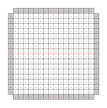
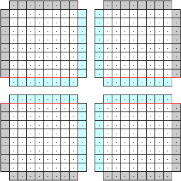
(a) (b)

Figure 1: Computational domain: (a) single domain with ghost cell zones; (b) decomposed domain with ghost cell zones for data exchanges between non-overlapping subdomains. Algorithm LABEL:alg:pfmm gives the main function for the block-based narrow band fast marching method. Apparently, all function calls are embedded in the for loop in order to be executed in each subdomain. As a simple way to run the sequential algorithm to obtain correct results, Algorithm 2.4 is placed in an infinite loop. The major addition in this loop not discussed above is the function that accesses the data of neighboring subdomains and integrates them into the heap if applicable. For convenience, let $\mathfrak{N}^{ib}$ represent the six neighboring blocks of block $ib$ (left, right, front, back, bottom, and top) and $\Pi^{ib}$ represent the collection of points that are corresponding to the ghost cell zones of its neighboring blocks. Therefore, as shown in Algorithm LABEL:alg:collect, $\varTheta^{ib}\cap\Pi^{nb}$ represents the portion of ghost cells in block $ib$ that are within the physical domain of block $nb$, If a point from $nb$ have a smaller function value, then its value and status can be copied to the corresponding point in block $ib$; this point will be added to $\mathfrak{H}^{ib}$ or its position in $\mathfrak{H}^{ib}$ will be adjusted for a current heap element. It is imperative that the infinite loop has a proper exit condition. Here we introduce a logical variable $\mathfrak{A}$ to indicate whether a subdomain $ib$ is active for further marching work ($\mathfrak{A}^{ib}=\texttt{TRUE}$) or not ($\mathfrak{A}^{ib}=\texttt{FALSE}$). As shown in Algorithm 2.1, $\mathfrak{A}^{ib}$ is initialized as FALSE and set to be TRUE if the subdomain has an nonempty initial heap. Then in Algorithm 2.4, same as the exit conditions for the sequential algorithm, when the heap is empty or the top element in the heap is beyond $\texttt{width}_{\text{band}}$, this block should be set inactive. On the other hand, a block has to be set active if its heap has any elements less than the terminal bound after integrating the data from neighboring blocks through ghost cells, as shown at the end of Algorithm LABEL:alg:collect. It is also required to include the KNOWN_NEW neighbors of a KNOWN point just removed from the heap in the check for possible updates, i.e., only KNOWN_FIX neighbors can be excluded from the check as shown in Algorithm 2. In addition, the quadratic equation is only solved at a neighbor with a larger value. Similar checks are imposed on looking for upwind points in Algorithm 3. These comparisons of function values added here for bypassing unnecessary computations would be redundant in the sequential algorithm, because points added to the KNOWN set follow a strict order of increasing function values if only a single domain is involved. As discussed above and in [yang2017highly] with more details, the sequential algorithm has not been altered by the introduction of the augmented status tags and these checks. However, they make the block-based algorithm a very natural extension of the sequential one.

2.4 Restarted narrow band approach

With the above block-based approach, it is clear that the sequential fast marching algorithm will run in each block until exit, then data will be exchanged among neighbors via ghost cells; and both the marching and exchanging steps repeat until the global exit condition is met. This is straightforward in concept and implementation, but the performance is unsatisfying by any means. In [yang2017highly], a novel restarted narrow band approach was proposed to address the performance issue by replacing the terminal narrow band bound $\texttt{width}_{\text{band}}$ with an evolving one, i.e., $\texttt{bound}_{\text{band}}$ in Algorithm 2.4. It should be noted here that the condition to label the block as inactive is still determined by $\texttt{width}_{\text{band}}$. On the other hand, as shown in Algorithm LABEL:alg:pfmm, a free parameter stride is introduced to advance the front by the extent of stride, or $\delta s$, in each run-through. Apparently, with $\texttt{stride}=\texttt{width}_{\text{band}}$ the previous block-based approach is fully restored. Algorithm 4 Front propagation within the narrow band:
$\textsc{March\_Narrow\_Band}{\color[rgb]{0,1,0}{(ib)}}$. 1:  $\Upsilon^{ib}\leftarrow\varnothing$ 2:  loop 3:     if $\texttt{size}(\mathfrak{H}^{\color[rgb]{0,1,0}{ib}})=0$ then 4:        $\mathfrak{A}^{ib}\leftarrow\texttt{FALSE}$ 5:        exit loop 6:     end if 7:     $(i,j,k)\leftarrow\textsc{Locate\_Min}(\mathfrak{H}^{\color[rgb]{0,1,0}{ib}})$ 8:     if $\psi {}^{ib}{}_{i,j,k}>\text{<span class="ltx\_rule" style="width:2.0pt;height:0.8pt;position:relative; bottom:2.2pt;background:black;display:inline-block;"> </span>}\text{width}{}_{\text{band}}\text{bound}{}_{\text{band}}\text{then}\text{<div id="alg4.l9nest" class="ltx\_listingline"> <span class="ltx\_tag ltx\_tag\_listingline"><span id="alg4.l9.1.1.1nest" class="ltx\_text" style="font-size:80\%;">9:</span></span><span id="alg4.l9.2nest" class="ltx\_text ltx\_font\_italic" style="color:\#0000FF;"> </span><span id="alg4.l9.3nest" class="ltx\_text ltx\_font\_bold" style="color:\#0000FF;">if</span>ψibi,j,k><span id="alg4.l9.9nest" class="ltx\_text ltx\_font\_typewriter" style="color:\#0000FF;">width</span><span id="alg4.l9.10.1.1.1nest" class="ltx\_text" style="font-size:70\%;">band</span><span id="alg4.l9.12nest" class="ltx\_text ltx\_font\_bold" style="color:\#0000FF;">then</span> </div>}\text{<div id="alg4.l10nest" class="ltx\_listingline"> <span class="ltx\_tag ltx\_tag\_listingline"><span id="alg4.l10.1.1.1nest" class="ltx\_text" style="font-size:80\%;">10:</span></span><span id="alg4.l10.2nest" class="ltx\_text ltx\_font\_italic" style="color:\#00FF00;"> </span>Aib←<span id="alg4.l10.6nest" class="ltx\_text ltx\_font\_typewriter" style="color:\#00FF00;">FALSE</span> </div>}\text{<div id="alg4.l11nest" class="ltx\_listingline"> <span class="ltx\_tag ltx\_tag\_listingline"><span id="alg4.l11.1.1.1nest" class="ltx\_text" style="font-size:80\%;">11:</span></span><span id="alg4.l11.2nest" class="ltx\_text ltx\_font\_italic" style="color:\#0000FF;"> </span><span id="alg4.l11.3nest" class="ltx\_text ltx\_font\_bold" style="color:\#0000FF;">end</span><span id="alg4.l11.5nest" class="ltx\_text ltx\_font\_bold" style="color:\#0000FF;">if</span> </div>}\text{<div id="alg4.l12nest" class="ltx\_listingline"> <span class="ltx\_tag ltx\_tag\_listingline"><span id="alg4.l12.1.1.1nest" class="ltx\_text" style="font-size:80\%;">12:</span></span><span id="alg4.l12.2nest" class="ltx\_text ltx\_font\_italic" style="color:\#0000FF;"> </span><span id="alg4.l12.3nest" class="ltx\_text ltx\_font\_bold" style="color:\#0000FF;">exit loop</span> </div>}\text{<div id="alg4.l13nest" class="ltx\_listingline"> <span class="ltx\_tag ltx\_tag\_listingline"><span id="alg4.l13.1.1.1nest" class="ltx\_text" style="font-size:80\%;">13:</span></span><span id="alg4.l13.2nest" class="ltx\_text ltx\_font\_italic" style="color:\#0000FF;"> </span><span id="alg4.l13.3nest" class="ltx\_text ltx\_font\_bold" style="color:\#0000FF;">end</span><span id="alg4.l13.5nest" class="ltx\_text ltx\_font\_bold" style="color:\#0000FF;">if</span> </div>}\text{<div id="alg4.l14nest" class="ltx\_listingline"> <span class="ltx\_tag ltx\_tag\_listingline"><span id="alg4.l14.1.1.1nest" class="ltx\_text" style="font-size:80\%;">14:</span></span><span id="alg4.l14.2nest" class="ltx\_text ltx\_font\_italic" style="color:\#FF0000;"> </span><span id="alg4.l14.3nest" class="ltx\_text ltx\_font\_bold" style="color:\#FF0000;">if</span>Gibi,j,k∉<span id="alg4.l14.9nest" class="ltx\_text ltx\_font\_typewriter" style="color:\#FF0000;">KNOWN\_FIX</span><span id="alg4.l14.11nest" class="ltx\_text ltx\_font\_bold" style="color:\#FF0000;">then</span> </div>}\text{<div id="alg4.l15nest" class="ltx\_listingline"> <span class="ltx\_tag ltx\_tag\_listingline"><span id="alg4.l15.1.1.1nest" class="ltx\_text" style="font-size:80\%;">15:</span></span><span id="alg4.l15.2nest" class="ltx\_text ltx\_font\_italic" style="color:\#000000;"> </span>G </div>}$