Numerical calculation of the full two-loop electroweak corrections to muon ($g$-2)

Abstract

Numerical calculation of two-loop electroweak corrections to the muon anomalous magnetic moment ($g$-2) is done based on, on shell renormalization scheme (OS) and free quark model (FQM). The GRACE-FORM system is used to generate Feynman diagrams and corresponding amplitudes. Total 1780 two-loop diagrams and 70 one-loop diagrams composed of counter terms are calculated to get the renormalized quantity. As for the numerical calculation, we adopt trapezoidal rule with Double Exponential method (DE). Linear extrapolation method (LE) is introduced to regularize UV- and IR-divergences and to get finite values. The reliability of our result is guaranteed by several conditions. The sum of one and two loop electroweak corrections in this renormalization scheme becomes $a_{\mu}^{EW:OS}[1{\rm+}2\mathchar 45\relax{\rm loop}]=151.2(\pm 1.0)\times 10^{-11}$, where the error is due to the numerical integration and the uncertainty of input mass parameters and of the hadronic corrections to electroweak loops. By taking the hadronic corrections into account, we get $a_{\mu}^{EW}[1{\rm+}2\mathchar 45\relax{\rm loop}]=152.9(\pm 1.0)\times 10^{-11}$. It is in agreement with the previous works given in PDGTanabashi et al. (2018) within errors.

I Introduction

In order to get a sign of beyond the standard model physics from high precision experimental data, we need higher order radiative corrections within Standard Model (SM). For this purpose our group has been developing the automatic calculation system GRACE [Yuasa et al., 2000] since the late 1980’s. The measurement of the muon anomalous magnetic moment $a_{\mu}\equiv(g\mathchar 45\relax 2)/2$ is the one of the most precise experiments to check the SM. QED correction was calculated by T.Kinoshita et al.[Aoyama et al., 2012] up to tenth-order. The two-loop electroweak (ELWK) correction to $a_{\mu}$ was calculated approximately by Kukhto et al.[Kukhto et al., 1992] in 1992. Surprisingly, the two-loop correction is almost 20% of the one-loop correction [Jackiw and Weinberg, 1972; Altarelli et al., 1972; Bars and Yoshimura, 1972; Fujikawa et al., 1972]. We started to calculate the full two-loop corrections in 1995 and presented our formalism at Pisa conference [Kaneko and Nakazawa, 1995]. We also showed that the two-loop QED value [Karplus and Kroll, 1950; Sommerfield, 1957; Petermann, 1957; C.M.Sommerfield, 1958] was correctly reproduced within our general formalism. However, the number of diagrams is huge and the numerical integration requires the big CPU-power to achieve required accuracy, we must wait until various environments are improved.

During these days, the several groups did the approximate calculations [Czarnecki et al., 1995, 1996, 2003; Gribouk and Czarnecki, 2005; Gnendiger et al., 2013; Heinemeyer et al., 2004] and the approximate value of the two-loop ELWK correction is widely accepted [Tanabashi et al., 2018,Marquard, 2015]. In 2001, BNL-Experiment 821 [Bennett et al., 2002,Bennett et al., 2004] announced that the precise experimental value deviates from that of SM around $(2.2\sim 2.7)\sigma~{}$[Bennett et al., 2006]. It brought much interest in the theoretical value. The main theoretical concern is now shifted to the hadronic contributions [Davier et al., 2011,Prades et al., 2009]. However, the discrepancy between the experimental value and the theoretical value is still large $\sim 3.5\sigma$ [Tanabashi et al., 2018,Mohr et al., 2012]. As new experiments at FNAL-E989 [Chapelain, 2017] will announce their first result in 2019 and J-PARC-E034 [Otani, 2015] is also planning the new experiment, we can expect to have a new data soon.

I.1 Perturbative Numerical QFT

Although the two-loop ELWK correction is almost established, we try to get the value without any approximation to confirm the validity of the earlier studies . This work is an important milestone to extend GRACE-system from one-loop to two-loop calculation. In ELWK theory, there are so many fields, mass parameters and complex couplings that it is hard to get reliable higher order corrections to physical quantities, in general. It is desirable to construct the framework to calculate these higher order corrections as automatically as possible. The key point is to perform Feynman integration numerically by using a sophisticated method with good convergence and high power CPU machine. We propose to call such framework as Perturbative Numerical Quantum Field Theory (PNQFT). The concepts of PNQFT are based on the following principles.

(a)

It is essential to assume amplitudes as meromorphic functions of space time dimension $n$ for regularization and getting gauge invariant renormalized values of physical quantities.

(b)

The source program for numerical integration is automatically generated by GRACE together with a symbolic manipulation system such as FORM [Vermaseren, 2000].

(c)

A high precision numerical integration method should be adopted.

(d)

Linear Expansion method (LE) (see subsection III.2) [de Doncker et al., 2012,de Doncker et al., 2018] is crucial to extract both UV- and IR-divergences by taking advantage of the above analyticity. By LE method, we can expand the amplitude in any order of $\varepsilon(=2-n/2)$ (Laurent expansion), so that it is a powerful tool for higher order calculation.

(e)

To guarantee the validity of the calculation, several conditions must be cleared. An example is the cancellation of non-linear gauge (NLG) parameters.

(f)

It is crucial to reduce human intervention to avoid careless mistakes. We must minimize the handmade operations necessary for getting the physical quantities.

The following calculation is based on these principles. In section II and III, we briefly explain the flow and framework of our calculation. In section IV, we touch on our method of numerical calculation. We emphasize that the Linear Extrapolation (LE) method is simple and efficient method to regularize UV- and IR-divergences and also to get finite values. We also explain our consistency conditions to ensure the results. Some examples of calculations are explained. In section V, we give our results on $a_{\mu}$ . In the last section, we give some comments to make extensive progress. In Appendices, we explain the technical parts of our calculation.

II Outline of our frame work

Our calculation is formulated under the following conditions.

1. The calculation is done within SM.

2. On mass shell renormalization scheme (OS) is adopted [Aoki et al., 1982; Fujimoto et al., 1990; Belanger et al., 2006]. We adopt $\alpha,M_{Z},M_{W},M_{H}$ and fermion masses as physical parameters. Weinberg angle, Higgs fermion coupling and other quantities are expressed by these parameters.

3. Free quark model (FQM) is adopted and as for quarks, constituent masses are used.

4. Non-linear gauge formulation with ’t Hooft-Feynman propagator is adopted.

5. Dimensional regularization is applied for both Ultra Violet (UV)- and Infrared (IR)-divergences.

6. Linear Extrapolation method (LE) is fully used for regularization and getting finite values.

Next, we briefly explain the flow of our calculation.

1. GRACE system generates all the diagrams we need in SM, automatically [Kaneko, 1995]. There are 1780 two-loop diagrams and 70 one-loop diagrams composed of one-loop order counter term (CT). Two-loop order CT is not necessary in our case, because $a_{\mu}$ is not related to the charge renormalization part.

2. These 1780 diagrams are classified into 14 types of topology. Types of the topology are displayed in Fig.1. Among these types, some of them give the same contribution because of symmetry. (an example: 5-a vs. 5-b) The diagrams including CT are classified into two types, namely, vertex and self-energy types.
   

   

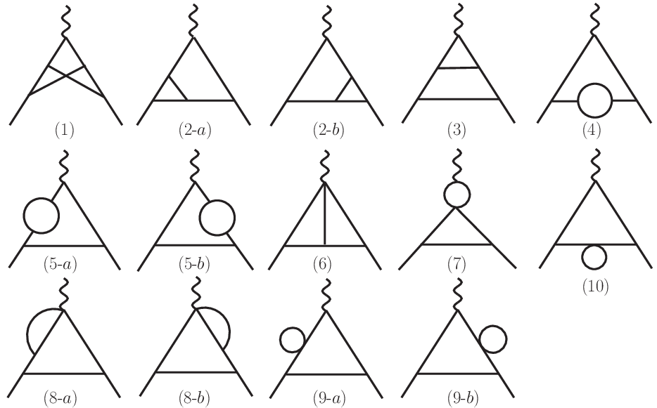
   Figure 1: Types of topology

3. GRACE system generates the amplitude of each diagram in accordance with Feynman rules for ELWK theory with NLG [Belanger et al., 2006].

4. In order to express the amplitude as a function of Feynman parameters used to combine denominators, we define the following quantities for each topology in advance [Cvitanovic and Kinoshita, 1974a,Cvitanovic and Kinoshita, 1974b].

   • Internal loop momentum flow$(\ell_{s},\eta(s))$ ($s=1,2$)

   • External momentum flow $(q_{j})$ ($j=$ internal line number)

   • Kirchhoff’s law of momentum conservation at each vertex

   • Feynman parameters are transformed to the integration variables in the interval [0,1].

5. Using these tools, contribution of each diagram to $a_{\mu}$ is expressed as function of Feynman parameters, according to the formulas given in the next section. We make use of a symbolic manipulation system FORM exhaustively.

III Logic of the Calculation

III.1 Cvitanovi$\acute{\rm c}$-Kinoshita procedure

In order to extract $a_{\mu}$ factor from muon vertex function, we adopt Cvitanovi$\acute{\rm c}$-Kinoshita procedure [Cvitanovic and Kinoshita, 1974a,Cvitanovic and Kinoshita, 1974b]. We briefly explain the procedure in the case where there are six propagators. Starting formula is the two-loop muon vertex,

$$\Gamma_{\mu} = \int\frac{d^{n}\ell_{1}}{i(2\pi)^{n}}\frac{d^{n}\ell_{2}}{i(2\pi)^{n}}\frac{F_{\mu}(D)}{\prod_{j}(p_{j}^{2}-m_{j}^{2})}$$ (1)

$$= \Gamma(6)\int\prod dz_{j}\delta(1-\sum_{j}z_{j})$$

$$\times \int\frac{d^{n}\ell_{1}}{i(2\pi)^{n}}\frac{d^{n}\ell_{2}}{i(2\pi)^{n}}\frac{F_{\mu}(D)}{\sum_{j}z_{j}(p_{j}^{2}-m_{j}^{2})}$$

where $\displaystyle{p_{j}=\sum_{s=1}^{2}\eta_{s}(j)\ell_{s}+q_{j}}$, is the momentum on the internal line $(j)$. The function $\eta_{s}(j)(=\pm 1,0)$ defines the weight of loop momentum $\ell_{s}$ on the internal line $(j)$. The $z_{j}$’s are the Feynman parameters to combine six propagators. $F_{\mu}(D)$ is the numerator function and $\mu$ is the external photon polarization. Next we diagonalize the denominator function with respect to loop momenta $\ell_{1}$, $\ell_{2}$ and perform integration. The result is,

$$\Gamma_{\mu} = \frac{1}{(4\pi)^{n}}\int\prod dz_{j}\delta(1-\sum_{j}z_{j})\frac{\Gamma(6-n)}{({\rm detU})^{n/2}}$$

$$\times F_{\mu}(D)\frac{1}{(V-i\epsilon)^{6-n}},~{}~{}U_{s,t}=\sum_{j=1}^{6}z_{j}\eta_{s}(j)\eta_{t}(j).$$

Where ${U}$ is well known 2$\times$2 matrix, composed of Feynman parameters $(z_{j})$. $V(z_{j},m_{j},q_{j})$ is the denominator function. The argument is easily extended to the case with five-propagators (diagrams with four-point coupling).

In order to generate the numerator function we use the following differential integral operator $D^{\mu}_{j}$.

$$\frac{p_{j}^{\mu}}{(p_{j}^{2}-m_{j}^{2})}=D_{j}^{\mu}\frac{1}{(p_{j}^{2}-m_{j}^{2})},~{}D_{j}^{\mu}\equiv\frac{1}{2}\int\nolimits_{m_{j}^{2}}^{\infty}dm_{j}^{2}\frac{\partial}{\partial q_{j\mu}}$$

The operator $D_{j}^{\mu}$ generates momentum $p_{j}^{\mu}$ on the internal line $(j)$. By operating $D_{j}^{\mu}$ to the denominator function $V$, we get the following expression.

$$D_{i}^{\mu}D_{j}^{\nu}\frac{1}{V^{m}} = \frac{Q_{i}^{\mu}Q_{j}^{\nu}}{V^{m}}+\left(-\frac{1}{2\rm detU}\right)\frac{g^{\mu\nu}}{(m-1)}\frac{B_{ij}}{V^{m-1}}$$ (4)

$${Q}_{j}^{\mu} = q_{j}^{\mu}-\frac{1}{{\rm det}U}\sum_{i=1}^{6}z_{i}B_{ij}q_{i}^{\mu}$$ (5)

$$B_{ij} = \sum_{s,t}\eta_{s}(i)\eta_{t}(j)U^{-1}_{st}{\rm det}U=B_{ji}$$ (6)

Using the above formulas, we can write down the numerator functions in terms of $B_{ij}$ algebraically. The equivalence of the above method and the well known method of shifting loop momentum to diagonalize the denominator function is verified. The correspondence between two methods are symbolized as follows.

$$\ell^{0}~{} \rightarrow ~{}\frac{\{1,Q_{i}^{\mu},Q_{i}^{\mu}Q_{j}^{\nu},\cdots\}}{V^{m}},$$

$$\ell_{i}^{\mu}\ell_{j}^{\nu}~{} \rightarrow ~{}~{}\left(-\frac{1}{2{\rm detU}}\right)\frac{g^{\mu\nu}}{(m-1)}\frac{B_{ij}}{V^{m-1}}$$ (7)

Next step is to extract the $a_{\mu}$ factor by using projection operator, from the photon muon vertex $\Gamma_{\mu}$. The quantity $a_{\mu}$ is given as follows. ( $m_{0}$=muon mass )

$$a_{\mu} = \lim_{q^{2}\rightarrow 0}\frac{{m_{0}}}{p^{4}q^{2}}{\rm Tr}\left(\Gamma_{\mu}{\rm Proj}(\mu)\right)$$

$${\rm Proj}(\mu) = \frac{1}{4}(\hbox to0.0pt{/\hss}p-{1\over 2}\hbox to0.0pt{/\hss}q+m_{0})\{{\rm m_{0}}\gamma_{\mu}(p.p)-({m_{0}}^{2}+\frac{q.q}{2})p_{\mu}\}$$ (8)

$$\times (\hbox to0.0pt{/\hss}p+{1\over 2}\hbox to0.0pt{/\hss}q+{\rm m_{0}}),~{}~{}~{}$$

where we set momentum of incoming $\mu^{-}$, outgoing $\mu^{-}$ and incoming photon, as $(p-q/2),(p+q/2)$ and $q$, respectively.
The final expression for numerical integration is summarized in the following formula.

$$F = \frac{1}{(4\pi)^{n}}\int\prod dz_{j}\delta(1-\sum_{j}z_{j})$$ (9)

$$\times \left[\frac{\Gamma(6-n)f_{0}}{({\rm detU})^{n/2}(V-i\epsilon)^{6-n}}\right.$$

$$+ \left.\frac{\Gamma(5-n)f_{2}}{-2({\rm detU})^{n/2+1}(V-i\epsilon)^{5-n}}\right]$$

The numerators $f_{0},f_{2}$ represent the coefficient of $\ell^{0},\ell^{2}$ term, respectively, after projection operator is applied. They are also the function of dimension $n$.

III.2 Regularization Method

Next step is the regularization of UV- and IR-divergences. By adopting $n$-dimensional regularization method, any integrand $F$ of Feynman parameter integration is regarded as a function of $\varepsilon=2-n/2,~{}F(\varepsilon)$. We adopt two methods for regularization.

III.2.1 Linear Expansion method

First one is very simple and powerful if the accuracy of numerical integration is sufficiently guaranteed. We call it Linear Expansion method (LE). Just after the dimensional regularization method was introduced [Bollini and Giambiagi, 1972,’t Hooft and Veltman, 1972], the analyticity with respect to $\varepsilon$ was discussed extensively. It is shown that the Feynman amplitude is a meromorphic function of $\varepsilon$ [Bollini and Giambiagi, 1972,’t Hooft and Veltman, 1972,N.Nakanishi, 1975]. This is a key point to utilize the LE-method to the Feynman amplitude. The followings are the steps to get the divergent and finite terms.

1. Calculate $G(\varepsilon)=\int F(z_{j},\varepsilon)\prod dz_{j}$ for various values of $\varepsilon=\varepsilon(i)$.  $(i=1,2,\cdots M)$.

2. We set $\varepsilon(i)=1/\alpha^{i+14}$ by taking relevant value $\alpha$.

3. According to the analyticity, we can expand $G(\varepsilon(i))$ in Laurent series. In our case, it is evident that the expansion starts from $(1/\varepsilon(i))$ because of the lack of two-loop counter terms. We truncate the series at O($\varepsilon(i)^{M-2}$).

   $$G(\varepsilon(i)) = C_{-1}\frac{1}{\varepsilon(i)}+C_{0}+C_{1}\varepsilon(i)+\cdots+C_{M-2}\varepsilon(i)^{M-2}$$ (10)

   $$= \sum_{j=-1}^{M-2}C_{j}\{\varepsilon(i)\}^{j}~{}~{}~{}~{}(i=1,2,\cdots M)$$

   The coefficients $C_{-1}$ and $C_{0}$ correspond to the divergent and finite parts, respectively. In the case $\varepsilon=2-n/2$, $C_{-1}$ expresses the UV-divergent part and if we set $\varepsilon\rightarrow\varepsilon_{R}=(n/2-4),C_{-1}$ represents the IR-divergent part.

4. To get $\{C_{j}\}$, we multiply the inverse of $M\times M$ matrix $A$, whose element is $A(i,j)=\{\varepsilon(i)\}^{j},~{}(i=1,\cdots M,~{}j=-1,0,\cdots,M\mathchar 45\relax 2)$, to M-component vector $G(\varepsilon(i))$.

   $$C_{j}=\sum_{i=1}^{M}A^{-1}(j,i)G(\varepsilon(i)),~{}~{}(j=\mathchar 45\relax 1,0,\cdots,M\mathchar 45\relax 2)$$ (11)

5. In order to improve the convergence, we set $M\sim 18$ and $\alpha\sim 1.1$ by trial and error. Examples setting these parameters are shown in [de Doncker et al., 2012,de Doncker et al., 2018]

6. Various methods are known to extract $C_{-1},~{}C_{0}$ from $G(\varepsilon(i))$ [Sidi, 2003], however, LE method is simple and appropriate in our case.

In order to get the reliable value of $C_{-1},C_{0}$ up to 4 digits, we need the accuracy of the numerical integration at least 8 digits.

III.2.2 Subtraction Method

To complement the above calculation, we also adopt the well known subtraction method to separate divergent part and finite part. We extract $1/\varepsilon$  singularity from $G(\varepsilon)$ when one of Feynman parameters approaches 0, ($x\rightarrow 0$). The followings are the steps to extract the singularity.

1. First we transform the Feynman parameters $(z_{1},z_{2},\cdots,z_{6})$ into the appropriate [0,1] variables $(x,y,u,v,w)$ depending on the topology. Key point is to factorize the function detU=$x\times z(x,\cdots)$, where $z(0,\cdots)\neq 0$ . Singular behavior $(1/\varepsilon)$ comes from the factor (detU)^n/2 in Eq.(III.1)

2. The following formula is effective to extract the factor $(1/\varepsilon)$ for vertex type correction.

   $$I = \int_{0}^{1}x^{\varepsilon-1}F(x,\varepsilon)dx=\frac{1}{\varepsilon}F(0,0)+\frac{\partial F(0,0)}{\partial\varepsilon}$$ (12)

   $$+ \int_{0}^{1}\frac{F(x,0)-F(0,0)}{x}dx+O(\varepsilon)$$

3. In the case where there is self-energy type diagram, the factor $x^{\varepsilon-2}$ appears in the head of integrant. If we expand it in $\varepsilon$ by using analytic continuation the following formula is obtained.

   $$I = \int_{0}^{1}x^{\varepsilon-2}F(x,\varepsilon)dx$$ (13)

   $$= \frac{1}{\varepsilon}\frac{\partial F(0,0)}{\partial x}+\frac{\partial F(0,0)}{\partial x}+\frac{\partial^{2}F(0,0)}{\partial\varepsilon\partial x}-F(1,0)$$

   $$+ \int\nolimits_{0}^{1}\frac{{\partial F(x,0)}/{\partial x}-{\partial F(0,0)}/{\partial x}}{x}dx+O(\varepsilon)$$

We use this method partly to complement the LE method.

III.2.3 Counter terms

As for counter terms, GRACE has a library of renormalization constants at one-loop level based on OS-renormalization scheme. We make use of this library for 70-diagrams composed of counter terms. Generally speaking, it is necessary to expand one-loop renormalization constants up to order $\varepsilon=2-n/2$ at two-loop level. However, the divergent part of diagrams composed of CT does not contribute to $a_{\mu}$ , the $O(\varepsilon)$ term is unnecessary in our case. Here we comment on the wave function renormalization constant of goldstone fields $\chi,\chi_{3}$. We keep the finite part of the constant in the form $(-1/2)\{d\Pi^{\chi\chi}(q^{2})/dq^{2}\}~{}at~{}q^{2}=M_{W}^{2}$. However, the final answer is independent of the finite part. For the renormalization of unphysical fields, the UV-divergent part is only useful to erase divergence.

IV Numerical Calculation

IV.1 Double exponential method

The final step to get the value $a_{\mu}$ is the numerical integration over Feynman parameters. We employ trapezoidal rule with Double Exponential (DE) transformation method [H.Takahashi and M.Mori, 1974]. It is also called as $tanh$-$sinh$ transformation method. It is very powerful if the integrand has singular behavior at the edge of the integration domain. Speed of convergence is accelerated by the DE transformation,

$$I=\int_{0}^{1}dxf(x)\rightarrow x=\phi(t)={1\over 2}\left\{1+\tanh\left(\frac{\pi}{2}\sinh(t)\right)\right\}$$

The maximum dimension of multiple integration is five. We apply DE-method to any integration variable involved. As we need the accuracy greater than 8 digits to see the UV cancellation, the adaptive Monte Carlo method is not adopted in our two-loop calculation.

IV.2 Criterion to ensure the validity of the result

In order to ensure the validity of our results, we impose several conditions given below.

1. Well known QED two-loop value is reproduced up to 7 digits.

2. UV-divergence is cancelled.

3. IR-divergence is cancelled.

4. The result is independent of non-linear gauge parameters.

5. In some cases (examples: topology 4,5-a,5-b,7,9-1,9b and 10) , we can perform loop-integrations $\ell_{1}$ and $\ell_{2}$ successively. (We call it successive method.) We obtain the same value as the direct method previously shown.

In all these cases, if we have plural methods to evaluate, we compare the numerical values to ascertain the validity. We demonstrate how the conditions are cleared by showing the examples in Appendices.

IV.2.1 Non-linear gauge (NLG) parameter independence

Originally non-linear gauge was introduced to reduce the number of diagrams, particularly containing boson-boson couplings [Fujikawa, 1973; Joglekar, 1974; Shizuya, 1976; Das, 1982; Romao and Barroso, 1987; Boudjema and Chopin, 1996]. Here, we adopt NLG to check the validity of our calculation. The gauge fixing Lagrangian is constructed as,

$$\mathscr{L}_{GF}=-\frac{1}{\xi_{W}}F^{+}F^{-}-\frac{1}{2\xi_{Z}}(F^{Z})^{2}-\frac{1}{\xi}(F^{A})^{2}$$ (15)

where

$$F^{\pm} = \left(\partial^{\mu}\mp ie\tilde{\alpha}A^{\mu}\mp i\frac{ec_{W}}{s_{W}}\tilde{\beta}Z^{\mu}\right)W_{\mu}^{\pm}$$

$$+ \xi_{W}\left(M_{W}\chi^{\pm}+\frac{e}{2s_{W}}\tilde{\delta}H\chi^{\pm}\pm i\frac{e}{2s_{W}}\tilde{\kappa}\chi_{3}\chi^{\pm}\right)$$

$$F^{Z} = \partial^{\mu}Z_{\mu}+\xi_{z}\left(M_{Z}\chi_{3}+\frac{e}{2s_{W}c_{W}}\tilde{\varepsilon}H\chi_{3}\right)$$

$$F^{A} = \partial^{\mu}A_{\mu}$$ (16)

Here, $\tilde{\alpha},\tilde{\beta},\tilde{\delta},\tilde{\varepsilon}$ and $\tilde{\kappa}$ are non-linear gauge parameters specific to this formalism. The parameters $s_{W}$ and $c_{W}$ are the $sine$ and $cosine$ of Weinberg angle $\theta_{W}$. In our calculation we set $\xi=\xi_{W}=\xi_{Z}=1$ to make the gauge boson propagators simple. NLG parameters are distributed among so many diagrams of different types of topologies. So it is very powerful if we can verify the cancellation of these NLG parameters. We show the sample of cancellation in Appendix F.

IV.2.2 Successive method

Diagrams with self energy type two-point function can be calculated by successive method using renormalized two point function. An example is diagram with $(\gamma-\gamma)$ or $(\gamma-Z)$ vacuum polarization type diagrams. We decompose the renormalization constants $\delta Z_{AA}^{1/2},\delta Z_{ZA}^{1/2},\delta Z_{AZ}^{1/2},\delta M_{Z}^{2}$ etc. into components according to the particles involved in the loop. By adding the counter term to corresponding one-loop unrenormalized two-point function, one-loop ($\ell_{1}$) integration is performed without divergence and we obtain the renormalized two-point function $\Pi_{R}$. By inserting $\Pi_{R}$ into the second loop($\ell_{2}$), we get finite value of $a_{\mu}$ . We use this alternative method to reconfirm the results obtained by the methods given in section III. An example is shown in Appendix G.

V Results of our calculation

As the physical input parameters, we use the following fermion and boson masses (unit GeV).
$m_{\mu}=105.6583745\times 10^{-3}$, $m_{e}=0.5109989461\times 10^{-3}$, $m_{\tau}=1.77686$ $m_{u}=0.3$, $m_{c}=1.5$, $m_{t}=173.1$,$m_{d}=0.3$, $m_{s}=0.5$, $m_{b}=4.18$, $M_{W}=80.385$, $M_{Z}=91.1876$, $M_{H}=125.09$. We also choose the fine structure constant in the Thomson limit, $\alpha$ =1/137.035999139.

After clearing all the conditions given in section IV.2 we get the two-loop ELWK corrections to $a_{\mu}^{EW:OS}$[2-loop] in terms of $(\alpha,M_{Z},M_{W},M_{H},m_{f})$. The loop expansion is done by using $\alpha,\alpha^{2}$, successively. Among 1780 diagrams, we exclude 9 pure QED diagrams consisting of only $(e,\mu,\tau,\gamma)$ and 6 diagrams containing vacuum polarization composed of quark loop. Then the final result becomes,

$$a_{\mu}^{EW:OS}[2\mathchar 45\relax{\rm loop}]=(-36.76\pm 0.3)\times 10^{-11}.$$ (17)

The errors in the above and the following expressions are limited to the numerical integration error and the uncertainty of input parameters $M_{W},M_{H},M_{Z},m_{t},m_{b}$. The masses of light quarks are fixed in our model.

We show the fermionic and bosonic part of two loop correction separately for reference.

$$a_{\mu}^{EW:OS}[2\mathchar 45\relax{\rm loop}]_{\rm fermion} = -18.34(\pm 0.2)$$ (18)

$$a_{\mu}^{EW:OS}[2\mathchar 45\relax{\rm loop}]_{\rm boson} = -18.42(\pm 0.1)$$ (19)

As we mentioned before, we adopt OS renormalization, however, the expression in the preceding works is parametrized using Fermi constant $G_{F}=1.1663787\times 10^{-5}~{}{\rm GeV}^{-2}$ and $\alpha$ Gnendiger et al. (2013).

The difference of the 2-loop correction between our value and that in $G_{F}$ parametrization is due to the fact that one loop correction in $G_{F}$ parametrization partially includes the $\alpha^{2}$ correction in our scheme.

So the comparison should be done to the sum of one- and two-loop. The one loop correction in our OS scheme is written down as follows.

$$a_{\mu}^{EW:OS}[1\mathchar 45\relax{\rm loop}]=\frac{\alpha m^{2}_{\mu}M_{Z}^{2}}{16\pi(M_{Z}^{2}-M_{W}^{2})M_{W}^{2}}\times$$

$$\left[\frac{5}{3}+\frac{1}{3}\left(\frac{4M_{W}^{2}}{M_{Z}^{2}}-3\right)^{2}+\mathscr{O}\left(\frac{m^{2}_{\mu}}{M_{W}^{2}}\right)+\mathscr{O}\left(\frac{m^{2}_{\mu}}{M_{H}^{2}}\right)\right]$$

We can carry out the numerical calculation without any approximation and get the value.

$$a_{\mu}^{EW:OS}[1\mathchar 45\relax{\rm loop}]=187.99(\pm 0.2)\times 10^{-11}$$ (21)

By summing up one and two loop weak corrections, our result is as follows.

$$a_{\mu}^{EW:OS}[1{\rm+}2\mathchar 45\relax{\rm loop}]=151.2(\pm 1.0)\times 10^{-11}$$ (22)

Here we add the error due to neglecting the uncertainty in electroweak loops involving hadrons.

When we compare our result with the value obtained by using $G_{F}$ parametrization, we need the naive free light quark model calculation with the same quark masses as ours. This is given in ref.Czarnecki et al. (2003). In this case the two loop correction becomes, $-42.97(\pm 1)\times 10^{-11}$. In the $G_{F}$ parametrization, the one loop correction becomes $194.80(\pm 0.01)\times 10^{-11}$Gnendiger et al. (2013), so that we get,

$$a_{\mu}^{EW}[1{\rm+}2\mathchar 45\relax{\rm loop}]_{\rm FQM}=151.8(\pm 1)\times 10^{-11}.~{}~{}~{}~{}$$ (23)

This is consistent with our value Eq.(22)

We also add a comment on the relation between the well known PDG value Tanabashi et al. (2018) shown below and our value. If we include the hadronic correction to light quark contribution, by adding the difference of the following expression Gnendiger et al. (2013),

$$a_{\mu}^{EW(2)}(e,\mu,u,c,d,s)=(-6.91\pm 0.20\pm 0.3)\times 10^{-11}$$

and the value quoted in the footnote belowCzarnecki et al. (2003), our value becomes as follows.

$$a_{\mu}^{EW}[1{\rm+}2\mathchar 45\relax{\rm loop}]=152.9(\pm 1)\times 10^{-11}$$ (25)

It is in agreement with the following PDG value Tanabashi et al. (2018) within errors.

$$a_{\mu}^{EW}=153.6(\pm 1)\times 10^{-11}$$ (26)

VI Discussions and Comments

We developed the system to calculate the full ELWK two-loop corrections to $a_{\mu}$ , by fully using GRACE and FORM on the basis of OS-scheme. The work we need beforehand is only to prepare several files which only depend on the type of the topology of diagrams as we explained in section III. We adopt the dimensional regularization to regularize UV- and IR-divergences and to get finite gauge invariant values of the physical quantity. To extract the $(1/\varepsilon)$ terms, we use Linear Expansion Method explained in sectionIII-B. This method is very simple and attractive, compared with the conventional method to take out the $(1/\varepsilon)$ term by extrapolating one of the Feynman parameters close to 0 . If we adopt the conventional method, it is crucial to introduce the most suitable transformations from $(z_{j})$ to [0,1] integration variables $(x,y,u,v,w)$. Furthermore, we need rather complex operations including differentiation of the amplitude, etc. As a result, the necessary CPU-time increases extensively.

In the case of Linear Expansion method (LE), however, the choice of integration variables is not sensitive to get the reliable results and this method decreases the number of operation drastically. It is sufficient to define the quantity as function of $\varepsilon(=2-n/2)$ . We only need to treat Dirac matrices and various vectors appeared in the numerator, in $n$-dimension. This is easily done by using symbolic manipulation system such as FORM. The operation is simple and we can make use of the resultant short sources for both UV-($\varepsilon>0$) and IR-($\varepsilon_{R}=-\varepsilon>0$) regularization and also to get finite results. We conclude that LE-method is the most simple and reliable method, at this moment. In order to get reliable physical value by this method, high precision numerical integration over Feynman parameters is inevitable. The DE-method introduced in section IV.1 is the suitable candidate.

Introduction of NLG-parameters makes the calculation very complex, however, it is very powerful to check the calculation of so called Boson contribution. The number of diagrams consisting of different types of topology are connected through NLG-parameters. The maximum number of diagrams mutually entangled reaches 864. So this is a very tough condition to be cleared.

By making use of these technical approaches mentioned above, we clear all the constraints given in section IV.2 . Namely, (i) reproduction of QED values, (ii)(iii) cancellation of UV-and IR-divergences, (iv) Independence of NLG-gauge parameters. We show some samples in Appendices how they are cleared.

The final value of the sum of one and two loop weak corrections is approximately the same as the one obtained by previous works using different parametrization.

Based on this work we can proceed to construct PNQFT(Perturbative Numerical Quantum Field Theory), which we discussed in section I.1. Wide range of application to ELWK higher loop expansion for several physical reactions will be opened. We expect that this work provides the fruitful foundation to formulate PNQFT.

Appendix A Reproduction of QED two-loop value

QED two-loop value is reproduced correctly.

		Unit =$(\alpha/\pi)^{2}$
Analytic expression		-0.328478996
0ur value		-0.328479821

Appendix B Classification of Diagrams to Check Numerical Values

In Fig.1, we show types of topology to formulate the two-loop contributions. However, in order to check the consistency of numerical values, it is useful to classify diagrams by distinguishing fermion and boson lines in each diagrams in Fig.1. We briefly figure out the classification method in Fig.2.

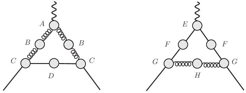
Figure 2: Classification of Diagrams

In the figure, the straight lines and wavy lines represent fermion and boson, respectively. The circle indicates one-loop diagram. We classify diagrams depending on the place where one-loop diagram is inserted. It is summarized in the following Table 1. You can easily see which one of Fig.1 is classified into which category.

Table 1: Classification of two loop diagrams. Depending on the position (A$\sim$H) of one loop diagram or one loop counter term, we give names shown below. For example, LAD-I and LAD-II correspond to topology (3) in Fig.1. The typical diagram belonging to LAD-I is fermion triangle with $\gamma\mathchar 45\relax\gamma\mathchar 45\relax Z$ legs.

A $\rightarrow$ LAD-I	B $\rightarrow$ SLF-I	C$\rightarrow$ VTX-1	D$\rightarrow$VCP-I
E$\rightarrow$ LAD-II	F$\rightarrow$ SLF-II	G$\rightarrow$ VTX-II	H$\rightarrow$ VCP-II
Fig.1(1) $\rightarrow$ CRL		Fig.1(6) $\rightarrow$ DBT

In the above Table 1 we add two types of topology having no divergence, namely, Fig.1-(1) and (6).

Appendix C UV-cancellation

In this Appendix, we show the cancellation of UV-divergence in linear gauge (’t Hooft-Feynman gauge). Examples of a group of diagrams are shown in Fig.3. The diagrams in Fig.3 belong to several groups in Table 1.

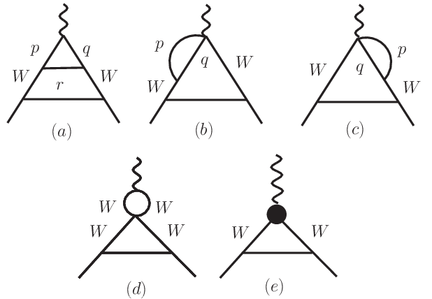
Figure 3: Sample diagrams with $W$

In this case, total 13-diagrams and 1-counter term (e) make a group to cancel UV-divergence. In the Table 2, the coefficient of $C_{UV}^{(2)}=(1/\varepsilon-2\gamma+2\ln(4\pi))$, corresponding to each diagram is shown. As you can read from the Table 2, the cancellation is marvelous, up to almost 15 digits.

Table 2: Sample of UV cancellation in ’t Hooft-Feynman gauge. UV cancellation is confirmed by summing up the coefficient of $C_{UV}^{(2)}$ of a set of diagrams. Here we show the set given in Fig.3 as a sample. The 15-digit cancellation is realized in the sum.

Diagram	Particles on	Value   $(\rm{unit~{}}10^{-11})$
in Fig.3	line $(p,q,r)$
(a)	$W-W-Z$	1.72758038865755734
(a)	$W-W-\gamma$	0.49552373441415571
(a)	$\chi-\chi-H$	0.05700266982235161
(a)	$\chi-\chi-\chi_{3}$	0.05700266982235161
(a)	$c^{-}-c^{-}-c^{Z}$	-0.02214846652125073
(a)	$c^{-}-c^{-}-c^{\gamma}$	-0.00635286838992507
(a)	$c^{+}-c^{+}-c^{Z}$	-0.02214846652125073
(a)	$c^{+}-c^{+}-c^{\gamma}$	-0.00635286838992507
(b)	$W-Z$	-0.17085951453900741
(b)	$W-\gamma$	-0.04900781767402955
(c)	$W-Z$	-0.17085951453900741
(c)	$W-\gamma$	-0.04900781767402955
(d)		-2.63840950598091337
(e)	CT ($\gamma-W-W$)	0.79803737751292251
	Sum	-0.00000000000000012

Appendix D IR-cancellation

LE method is applied to check IR-cancellation. Among two-loop diagrams, the 8 diagrams in Fig.(4) have IR-divergence. The diagrams with CT also have IR-divergence through $\delta Z_{W}^{1/2}$ (19 diagrams) and $\delta Z_{\mu}^{1/2}$ (28-diagrams). The IR-divergence at two-loop level is proportional to $C_{IR}^{(2)}=(-1/\varepsilon_{R}-2\gamma+2\ln(4\pi))$, $\varepsilon_{R}=(n/2-2)>0$. It is easily shown that the IR-divergence coming from $\delta Z_{W}^{1/2}$ cancels among the 19 CT-diagrams. As for the diagrams with $\delta Z_{\mu}^{1/2}$, IR-divergence is cancelled by the corresponding two-loop diagrams. We show coefficients of $C_{IR}^{(2)}$ in Table 3. The correspondence between small photon mass ($\lambda$) method and LE-method for IR-regularization is checked in the case of QED ladder diagram. Analytic value of a coefficient of $\ln(\lambda^{2}/m_{\mu}^{2})$ in unit of $(\alpha/\pi)^{2}$ is $(1/4)$ Karplus and Kroll (1950). It is 0.249999998 by our calculation using small photon mass. In LE-method, the coefficient of $C_{IR}^{(2)}$ becomes 0.249999999. We understand the correspondence between $\ln(\lambda^{2}/m_{\mu}^{2})$ and $C_{IR}^{(2)}$ is established. As we show in Table 3, no IR-divergence remains in the final expression.

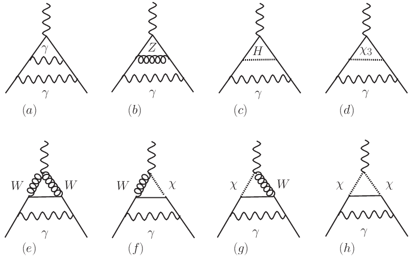
Figure 4: All the two-loop diagrams containing IR-divergence

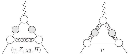
Figure 5: Diagrams containing IR-divergence through $\delta Z$. The straight lines and wavy lines represent fermion and boson, respectively. The circle represent $\delta Z_{\mu}^{1/2}$ or $\delta Z_{W}^{1/2}$. In the case where the corner includes $\nu$-particle, both of $\delta Z^{1/2}_{\mu},\delta Z^{1/2}_{W}$ are taken into account. The gray circles and white circles correspond to Self CT and Vertex CT in Table 3 , respectively.

Table 3: Cancellation of IR-divergence is shown. IR cancellation is confirmed by summing up the coefficient of $C_{IR}^{(2)}$. All the diagrams having IR-divergence are shown in FIG.4. Typical diagrams having IR-divergence through the renormalization constants are shown in FIG.5.

Type of correction	Numerical Value (unit $10^{-11}$)
Diagram Type	$\delta Z_{\mu}^{1/2}$ Vertex CT	$\delta Z_{\mu}^{1/2}$ Self CT	two-loop diagram	sum
Neutral Type			diagram
$\gamma$	$-134887.2756\times 3$	$134887.2756\times 2$	(a) $+134887.2755$	$-1.6\times 10^{-4}$
$Z-boson$	$0.217294\times 3$	$-0.217294\times 2$	(b) $-0.217294$	$-2.0\times 10^{-9}$
$Higgs,\chi_{3}$	$1.67970\times 10^{-6}\times 3$	$-1.67970\times 10^{-6}\times 2$	$(c,d)-1.67970\times 10^{-6}$	$2.6\times 10^{-13}$
Charged type
$W^{\pm},\chi^{\pm}$	-0.435625	$----$	(e)$\sim$(h) 0.435625	$+3.4\times 10^{-12}$

Appendix E Sample calculation of the two-loop diagram

As a sample, we show the calculation of the two-loop diagram which contains both UV- and IR-divergences. The diagram is shown in Fig.4-(b). The line numbers are given in Fig.6. Following Eq.(9) given in section III-A, the essential part of expression of two-loop diagram contribution is written as the following form.

$$F_{0} = \int\prod dz_{j}\left[\frac{1}{({\rm detU})^{-3\varepsilon}}\frac{f_{0}}{(\mathscr{D}-i\epsilon)^{2+2\varepsilon}}\right]$$ (27)

$$F_{2} = \int\prod dz_{j}\left[\left(-{1\over 2}\right)\frac{1}{({\rm detU})^{2-3\varepsilon}}\frac{f_{2}}{(\mathscr{D}-i\epsilon)^{1+2\varepsilon}}\right]$$

Quantities in Eq.(27),(E) are expressed by Feynman parameters $z_{j},~{}(j=1,\cdots,6)$, ($\sum_{j}z_{j}=1$). Masses are made dimensionless using muon mass.

$$V=-z_{5}+z_{5}^{2}(z_{23}+z_{6})/{\rm detU}+z_{1234}+z_{6}M_{Z}^{2}$$

$${\rm detU}=z_{6}z_{12345}+z_{3}z_{45}+z_{2}z_{145}+z_{1}z_{3}$$

$$\mathscr{D}\equiv{\rm detU}\times V=(z_{14}+z_{23})z_{14}z_{23}+z_{23}^{2}z_{5}$$

$$~{}~{}~{}~{}+(z_{14}+z_{23})^{2}z_{6}+(z_{6}M_{Z}^{2}){\rm detU}$$ (29)

where $z_{ij\cdots k}=z_{i}+z_{j}+\cdots+z_{k}$. Functions $f_{0},f_{2}$ are expanded in $\varepsilon$ up to $O(\varepsilon)$.

$$f_{0}=f_{00}+\varepsilon f_{01},~{}f_{2}=f_{20}+\varepsilon f_{21},~{}\varepsilon=(2-n/2)~{}~{}~{}$$ (30)

The $f_{0}$ and $f_{2}$ part give IR- and UV-divergences, respectively. By adopting DE and LE methods for Feynman parameter integration, we get the following expansion. ($\varepsilon_{R}=-\varepsilon$)

$$F_{0} \rightarrow \left(\frac{C_{-1}}{-\varepsilon_{R}}+C_{0}+C_{1}(-\varepsilon_{R})+\cdots\right)$$

$$F_{2} \rightarrow \left(\frac{D_{-1}}{\varepsilon}+D_{0}+D_{1}\varepsilon+\cdots\right)$$

We multiply the $\Gamma$ functions arising from n-dimensional integration and factor $1/(4\pi)^{n}$ , to the above quantities,

$$\frac{\Gamma(6-n)}{(4\pi)^{n}}F_{0} \rightarrow \left[C_{-1}C_{IR}^{(2)}+2C_{-1}+C_{0}+O(\varepsilon_{R})\right]$$

$$\frac{\Gamma(5-n)}{(4\pi)^{n}}F_{2} \rightarrow \left[D_{-1}C_{UV}^{(2)}+D_{0}+O(\varepsilon)\right]$$ (31)

We must pay attention that the term $(2C_{-1})$ appears, because $\Gamma(6-n)$ contains the term $(1-2\varepsilon_{R})$. In order to get the correct finite value, we must calculate the counter terms using the same regularization method for both IR- and UV-divergences as in two-loop case. In this case, we need muon wave function renormalization constant $\delta Z_{\mu}$. The $\delta Z_{\mu}$ is obtained by calculating muon self energy diagrams. The $\delta Z_{\mu}(\gamma)$ represents photon exchange part and $\delta Z_{\mu}(Z)$ represents Z-exchange part.

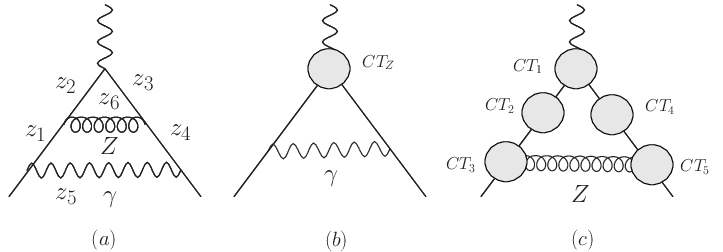
Figure 6: Diagram containing both UV- and IR-divergences. $CT_{Z},CT_{1}\sim CT_{5}$ represent the CT-terms.

In Fig.6-(b), $CT_{Z}$ represents $\delta Z_{\mu}(Z)$, and in Fig.6-(c), $CT_{1}\sim CT_{5}$represent only IR-divergent part of $\delta Z_{\mu}(\gamma)$. These IR-divergent part cancels that of Fig.6-(a) as is shown in the Table 3. We will show the numerical results to see the situation clearly. (unit=$10^{-11}$)

$$C_{-1} = -0.217294$$

$$C_{0} = ~{}~{}1.672727$$

$$D_{-1} = ~{}~{}24621.375584$$

$$D_{0} = -246732.662539$$ (32)

The term $CT_{Z}$ has both UV and finite parts.

$$(CT_{Z})_{UV} = -24621.375584$$

$$(CT_{Z})_{f} = ~{}~{}246728.863173$$ (33)

UV-cancellation is excellent and cancels 17 digits.

$$D_{-1}+(CT_{Z})_{UV}=3.84\times 10^{-12}$$ (34)

To cancel IR part of Fig.6-(a) , we adopt IR-part of $\delta Z_{\mu}(\gamma),CT_{1}\sim CT_{5}$. It is explained in the Table 3, row ($Z~{}~{}boson$). The finite value is obtained as follows.

$$C_{0}+2C_{-1}+D_{0}+(CT_{Z})_{f}=-2.561228$$ (35)

We can also regularize the IR divergent part by employing the small photon mass $\lambda^{2}$, to see $\log(\lambda^{2})$ term. As we notice that we must use the same regularization method for both two-loop and CT diagrams. At first sight, the finite part changes compared with dimensional regularization method, however, the sum of two-loop and CT contribution is the same in both regularization methods. We confirm it by numerical calculation.
As we can see from Eq.(35), we need very careful treatment to discuss order of (a few) $\times 10^{-11}$ quantity of $a_{\mu}$.

Appendix F NLG parameter cancellation

As an example of cancellation of NLG parameters, we show the UV-divergent part and finite part of diagrams which contain $\tilde{\alpha}^{n}~{}(n=1,2,3)$ terms. Total number of diagrams depending on $\tilde{\alpha}$ amount to 864. In order to see how the NLG-parameters are cancelled, we classify diagrams according to Fig.2 and Table 1. We summarize the result of numerical calculation in Table 4. In the last row in Table 4, we show the maximum absolute value among the individual terms in the column and its type of diagram, to indicate the degree of the cancellation. First we see the cancellation of the parameter $\tilde{\alpha}^{n}$ in the UV-divergent part, namely, the coefficients of $C_{UV}^{(2)}$. It is shown in the left half part of the Table 4. We can see the cancellation works very well and it strongly guarantees the validity of our numerical calculation. In the right half of Table 4, we also show the finite contribution to $a_{\mu}$. The column $\tilde{\alpha}^{1}\sim\tilde{\alpha}^{3}$ show that how the NLG-cancellation works well also in finite part.

Appendix G Successive method

In some cases, in order to check our calculation, we perform two-loop integrations successively. By integrating the first loop ($\ell_{1}$), we make the renormalized effective function and insert it to the second loop($\ell_{2}$) integration. As an example, we calculate the diagrams consisting of photon-Z meson mixing vacuum polarization. There are two types of topology 4 and 10 in Fig.1.
In general, unrenormalized two point $\gamma-Z$ function is written as follows.

$$\Pi(q^{2})^{un}_{\mu\nu}=\Pi^{un}_{T}(q^{2})\left(g_{\mu\nu}-\frac{q_{\mu}q_{\nu}}{q^{2}}\right)+\Pi^{un}_{L}(q^{2})\frac{q_{\mu}q_{\nu}}{q^{2}}$$

Each one-loop diagram contributes to $\Pi^{un}_{T}(q^{2}),\Pi^{un}_{L}(q^{2})$ in the following form.

$$\Pi_{T}^{un}(q^{2})=a(q^{2}),~{}~{}\Pi_{L}^{un}(q^{2})=a(q^{2})+q^{2}b(q^{2})$$ (37)

where

$$a(q^{2}) = \int\frac{d^{n}\ell}{i(2\pi)^{n}}\left[\frac{A_{1}\ell^{2}+(A_{2}q^{2}+A_{3})}{(\ell^{2}-D_{Q})^{2}}+\frac{A_{4}}{(\ell^{2}-m^{2})}\right]$$

$$b(q^{2}) = \int\frac{d^{n}\ell}{i(2\pi)^{n}}\frac{B}{(\ell^{2}-D_{Q})^{2}}$$ (38)

The variables $A_{1}\sim A_{4},B,D_{Q},m$ depend on the specific one-loop diagram. The $A_{4}$-term comes from the 4-point boson coupling diagram. However, this term drops out by the renormalization process.
In the followings, the renormalized quantity $\Pi$ are expressed as $\hat{\Pi}$.

$$\hat{\Pi}_{T}(q^{2}) = (M_{Z}^{2}-q^{2})\delta Z_{ZA}^{1/2}-q^{2}\delta Z_{AZ}^{1/2}+\Pi_{T}^{un}(q^{2})$$

$$\vspace{0.2cm}\hat{\Pi}_{L}(q^{2}) = M_{Z}^{2}\delta Z_{ZA}^{1/2}+\Pi_{L}^{un}(q^{2})$$

$$\vspace{0.2cm}\hat{\Pi}_{T}(q^{2} = 0)=0,~{}~{}~{}~{}\hat{\Pi}_{T}(q^{2}=M_{Z}^{2})=0$$ (39)

We notice that the renormalization conditions are fixed by $\Pi^{un}_{T}(q^{2})$, there is no freedom to renormalize $\Pi_{L}^{un}(q^{2})$. By using these renormalization conditions, we can write down renormalized $a_{R}(q^{2})$. It has no divergence, we can perform loop($\ell_{1}$) integration.

Table 4: Cancellation of NLG $\tilde{\alpha}$ parameter is shown. Numbers are in unit of $10^{-11}$. All the two-loop diagrams and CT terms are classified according to the TABLE II. Numbers represent the coefficients of $\tilde{\alpha},\tilde{\alpha}^{2},\tilde{\alpha}^{3}$ after summing up the contributions of both two-loop diagrams and CT terms. The last row shows the maximum absolute value within the same column and its topology type, to show how the cancellation works well.

Type of	Number of		Coefficient of $C_{UV}^{(2)}$ (unit  $10^{-11}$)			Finite contribution to (g-2) (unit  $10^{-11}$)
Diagrams	Diagrms		$\tilde{\alpha}$	$\tilde{\alpha}^{2}$	$\tilde{\alpha}^{3}$	$\tilde{\alpha}$	$\tilde{\alpha}^{2}$	$\tilde{\alpha}^{3}$
	2loop	CT
LAD-I	400	10	$1.3\times 10^{-11}$	-0.25876	-0.03235	6.11086	3.98570	0.83255
LAD-II	468	6	$-1.0\times 10^{-11}$			-0.12093
VTX-I	80	8	$1.1\times 10^{-16}$	$-5.7\times 10^{-16}$		1.16937	2.07396
VTX-II	90	8	$-4.7\times 10^{-11}$			-0.83645
SLF-I	312	16	$3.6\times 10^{-16}$	0.25876	0.03235	-3.48758	-3.87681	-0.83255
SLF-II	48	8
VCP-I	12	4	$-1.1\times 10^{-10}$	$-1.1\times 10^{-10}$
VCP-II	280	10				-0.05656	0.00074
CRL	72	0				-2.77731	1.18564
DBT	18	0					-3.36911
SUM	1780	70	$-1.65\times 10^{-10}$	$-1.42\times 10^{-10}$	$<1\times 10^{-30}$	0.00138	0.00012	$1.1\times 10^{-12}$
Type of diagram			VTX-II	LAD-I	SLF-I	VTX-I	LAD-I	SLF-I
Max. absolute value			$-298325.54724$	$-8.32905$	$-0.19407$	$2763874.32283$	$-46.38364$	$4.41044$

(*) Each contribution is calculated in quadruple precision method and has more effective digit than shown in the table.

The result is given as Eq.(40),(G). where $M$ represents the mass of a particle circulating the loop. As for $\hat{b}(q^{2})$, we must check whether it is really finite or not. The $C_{UV}$-part of $\hat{b}(q^{2})$ disappears after summing all the one-loop diagrams and integration of Feynman parameter $x$.

$$\hat{a}(q^{2}) = \hat{\Pi}^{AZ}_{T}(q^{2})=\left(\frac{1}{16\pi^{2}}\right)\int_{0}^{1}dx\int_{0}^{1}dz\left[A_{1}\{q^{2}(q^{2}-M_{Z}^{2})\}[x(1-x)^{2}]\frac{-2}{-zx(1-x)}\frac{1}{(q^{2}-M_{3}^{2})}\right.$$ (40)

$$+ A_{2}\{q^{2}(q^{2}-M_{Z}^{2})\}[x(1-x)]\frac{1}{-zx(1-x)}\frac{1}{(q^{2}-M_{2}^{2})}+A_{3}\{q^{2}\}[x(1-x)]\frac{1}{-zx(1-x)}\frac{1}{(q^{2}-M_{1}^{2})}$$

$$+ A_{3}\{q^{2}\}[x(1-x)]\left.\frac{-1}{V_{WZ}}\right]$$

$$M_{1}^{2} = \frac{M^{2}}{zx(1-x)},~{}~{}M_{2}^{2}=\frac{M^{2}}{zx(1-x)}-\frac{1-z}{z}M_{Z}^{2}M_{3}^{2}=\frac{M^{2}}{zx(1-x)}-\frac{y}{z}M_{Z}^{2},~{}~{}V_{WZ}=M^{2}-zx(1-x)M_{Z}^{2}$$

We also notice that the $\hat{b}(q^{2})$-part does not contribute to $a_{\mu}$, because it is proportional to $q_{\mu}q_{\nu}$.

Next step is to insert the renormalized two point function $\hat{a}(q^{2})g_{\mu\nu}$ into the triangle diagram and integrate over second loop momentum $\ell_{2}$. The integration has logarithmic divergent part, however, it drops out by the projection operator to $a_{\mu}$ , Eq.(8). Final expression is very complex and we do not quote here. From Eq.(40), we can see that there are denominators having $\ell_{2}(\leftarrow q)$. So the final expression has 5 integration parameters which run in the interval [0,1]. As a sample of calculation, we show sum of boson loop contribution. Fish type diagrams,{$(WW),(W\chi),(\chi W),(\chi\chi),(c^{+}c^{+}),(c^{-}c^{-})$} and tad pole type diagrams,$\{(W),(\chi),(c^{+}),(c^{-})\}$ composing $\Pi(q^{2})_{\mu\nu}$.

In unit of $10^{-11}$ we get, $-6.1048\times 10^{-3}$ by this method. On the other hand, we get $-6.104\times 10^{-3}$ by our two-loop formalism with CT-terms. The coincidence is quite good. Notice that, in this case the two-loop formalism takes huge cpu-time, especially for $(W-W)$ diagram. Its contribution is around $8.8\times 10^{6}$ in unit of $10^{-11}$ so that we need almost 15 digits number to cancel UV-divergence. So, the effective method is not only important to check the reliability of our general formalism but also is useful to get the numerical result. In the case of self-energy type diagrams, we can construct effective method in several cases, however, for vertex type diagrams, to construct effective method is complex.

References

- Tanabashi et al. (2018) M. Tanabashi et al. (Particle Data Group), Phys. Rev. D98, 030001 (2018).
- Yuasa et al. (2000) F. Yuasa et al., Computational physics and related topics. Proceedings, 5th International Conference, Kanazawa, Japan, October 11-13, 1999, Prog. Theor. Phys. Suppl. 138, 18 (2000), arXiv:hep-ph/0007053 [hep-ph] .
- Aoyama et al. (2012) T. Aoyama, M. Hayakawa, T. Kinoshita, and M. Nio, Phys. Rev. Lett. 109, 111807 (2012), arXiv:1205.5368 [hep-ph] .
- Kukhto et al. (1992) T. V. Kukhto, E. A. Kuraev, Z. K. Silagadze, and A. Schiller, Nucl. Phys. B371, 567 (1992).
- Jackiw and Weinberg (1972) R. Jackiw and S. Weinberg, Phys. Rev. D5, 2396 (1972).
- Altarelli et al. (1972) G. Altarelli, N. Cabibbo, and L. Maiani, Phys. Lett. 40B, 415 (1972).
- Bars and Yoshimura (1972) I. Bars and M. Yoshimura, Phys. Rev. D6, 374 (1972).
- Fujikawa et al. (1972) K. Fujikawa, B. W. Lee, and A. I. Sanda, Phys. Rev. D6, 2923 (1972).
- Kaneko and Nakazawa (1995) T. Kaneko and N. Nakazawa, in Artificial intelligence in high-energy and nuclear physics ’95. Proceedings, 4th International Workshop On Software Engineering, Artificial Intelligence, and Expert Systems, Pisa, Italy, April 3-8, 1995 (1995) pp. 0173–178, arXiv:hep-ph/9505278 [hep-ph] .
- Karplus and Kroll (1950) R. Karplus and N. M. Kroll, Phys. Rev. 77, 536 (1950).
- Sommerfield (1957) C. M. Sommerfield, Phys. Rev. 107, 328 (1957).
- Petermann (1957) A. Petermann, Helv. Phys. Acta 30, 407 (1957).
- C.M.Sommerfield (1958) C.M.Sommerfield, Ann.Phys.(NY) 5, 26 (1958).
- Czarnecki et al. (1995) A. Czarnecki, B. Krause, and W. J. Marciano, Phys. Rev. D52, R2619 (1995), arXiv:hep-ph/9506256 [hep-ph] .
- Czarnecki et al. (1996) A. Czarnecki, B. Krause, and W. J. Marciano, Phys. Rev. Lett. 76, 3267 (1996), arXiv:hep-ph/9512369 [hep-ph] .
- Czarnecki et al. (2003) A. Czarnecki, W. J. Marciano, and A. Vainshtein, Phys. Rev. D67, 073006 (2003), [Erratum: Phys. Rev.D73,119901(2006)], arXiv:hep-ph/0212229 [hep-ph] .
- Gribouk and Czarnecki (2005) T. Gribouk and A. Czarnecki, Phys. Rev. D72, 053016 (2005), arXiv:hep-ph/0509205 [hep-ph] .
- Gnendiger et al. (2013) C. Gnendiger, D. Stöckinger, and H. Stöckinger-Kim, Phys. Rev. D88, 053005 (2013), arXiv:1306.5546 [hep-ph] .
- Heinemeyer et al. (2004) S. Heinemeyer, D. Stockinger, and G. Weiglein, Nucl. Phys. B699, 103 (2004), arXiv:hep-ph/0405255 [hep-ph] .
- Marquard (2015) P. Marquard, Proceedings, 13th International Workshop on Tau Lepton Physics (TAU 2014): Aachen, Germany, September 15-19, 2014, Nucl. Part. Phys. Proc. 260, 107 (2015).
- Bennett et al. (2002) G. W. Bennett et al. (Muon g-2), Phys. Rev. Lett. 89, 101804 (2002), [Erratum: Phys. Rev. Lett.89,129903(2002)], arXiv:hep-ex/0208001 [hep-ex] .
- Bennett et al. (2004) G. W. Bennett et al. (Muon g-2), Phys. Rev. Lett. 92, 161802 (2004), arXiv:hep-ex/0401008 [hep-ex] .
- Bennett et al. (2006) G. W. Bennett et al. (Muon g-2), Phys. Rev. D73, 072003 (2006), arXiv:hep-ex/0602035 [hep-ex] .
- Davier et al. (2011) M. Davier, A. Hoecker, B. Malaescu, and Z. Zhang, Eur. Phys. J. C71, 1515 (2011), [Erratum: Eur. Phys. J.C72,1874(2012)], arXiv:1010.4180 [hep-ph] .
- Prades et al. (2009) J. Prades, E. de Rafael, and A. Vainshtein, Adv. Ser. Direct. High Energy Phys. 20, 303 (2009), arXiv:0901.0306 [hep-ph] .
- Mohr et al. (2012) P. J. Mohr, B. N. Taylor, and D. B. Newell, Rev. Mod. Phys. 84, 1527 (2012), arXiv:1203.5425 [physics.atom-ph] .
- Chapelain (2017) A. Chapelain (Muon g-2), Proceedings, 12th Conference on Quark Confinement and the Hadron Spectrum (Confinement XII): Thessaloniki, Greece, EPJ Web Conf. 137, 08001 (2017), arXiv:1701.02807 [physics.ins-det] .
- Otani (2015) M. Otani (E34), Proceedings, 2nd International Symposium on Science at J-PARC: Unlocking the Mysteries of Life, Matter and the Universe (J-PARC 2014): Tsukuba, Japan, July 12-15, 2014, JPS Conf. Proc. 8, 025008 (2015).
- Ishikawa et al. (2017) T. Ishikawa, N. Nakazawa, and Y. Yasui, Proceedings, 4th Computational Particle Physics Workshop (CPP2016): Hayama, Japan, October 8-11, 2016, J. Phys. Conf. Ser. 920, 012009 (2017), arXiv:1709.03284 [hep-ph] .
- Vermaseren (2000) J. A. M. Vermaseren, (2000), arXiv:math-ph/0010025 [math-ph] .
- de Doncker et al. (2012) E. de Doncker, F. Yuasa, and Y. Kurihara, Proceedings, 14th International Workshop on Advanced Computing and Analysis Techniques in Physics Research (ACAT 2011): Uxbridge, UK, September 5-9, 2011, J. Phys. Conf. Ser. 368, 012060 (2012).
- de Doncker et al. (2018) E. de Doncker, F. Yuasa, K. Kato, T. Ishikawa, J. Kapenga, and O. Olagbemi, Comput. Phys. Commun. 224, 164 (2018), arXiv:1702.04904 [hep-ph] .
- Aoki et al. (1982) K. I. Aoki, Z. Hioki, M. Konuma, R. Kawabe, and T. Muta, Prog. Theor. Phys. Suppl. 73, 1 (1982).
- Fujimoto et al. (1990) J. Fujimoto, M. Igarashi, N. Nakazawa, Y. Shimizu, and K. Tobimatsu, Prog. Theor. Phys. Suppl. 100, 1 (1990).
- Belanger et al. (2006) G. Belanger, F. Boudjema, J. Fujimoto, T. Ishikawa, T. Kaneko, K. Kato, and Y. Shimizu, Phys. Rept. 430, 117 (2006), arXiv:hep-ph/0308080 [hep-ph] .
- Kaneko (1995) T. Kaneko, Comput. Phys. Commun. 92, 127 (1995), arXiv:hep-th/9408107 [hep-th] .
- Cvitanovic and Kinoshita (1974a) P. Cvitanovic and T. Kinoshita, Phys. Rev. D10, 3978 (1974a).
- Cvitanovic and Kinoshita (1974b) P. Cvitanovic and T. Kinoshita, Phys. Rev. D10, 3991 (1974b).
- Bollini and Giambiagi (1972) C. G. Bollini and J. J. Giambiagi, Nuovo Cim. B12, 20 (1972).
- ’t Hooft and Veltman (1972) G. ’t Hooft and M. J. G. Veltman, Nucl. Phys. B44, 189 (1972).
- N.Nakanishi (1975) N.Nakanishi, Quantum Fiel Theory (in Japanese), page 271 (Baihukan,Tokyo, 1975).
- Sidi (2003) A. Sidi, Practical Extrapolation Method (Cambridge University Press, 2003).
- H.Takahashi and M.Mori (1974) H.Takahashi and M.Mori, Publ.RIMS Kyoto Univ. 9, 721 (1974).
- Fujikawa (1973) K. Fujikawa, Phys. Rev. D7, 393 (1973).
- Joglekar (1974) S. D. Joglekar, Phys. Rev. D10, 4095 (1974).
- Shizuya (1976) K.-i. Shizuya, Nucl. Phys. B109, 397 (1976).
- Das (1982) A. Das, Phys. Rev. D26, 2774 (1982).
- Romao and Barroso (1987) J. C. Romao and A. Barroso, Phys. Rev. D35, 2836 (1987).
- Boudjema and Chopin (1996) F. Boudjema and E. Chopin, Z. Phys. C73, 85 (1996), arXiv:hep-ph/9507396 [hep-ph] .