Targeted stochastic gradient Markov chain Monte Carlo for hidden Markov models with rare latent states

Abstract

Markov chain Monte Carlo (MCMC) algorithms for hidden Markov models often rely on the forward-backward sampler. This makes them computationally slow as the length of the time series increases, motivating the recent development of sub-sampling-based approaches. These approximate the full posterior by using small random subsequences of the data at each MCMC iteration within stochastic gradient MCMC. In the presence of imbalanced data resulting from rare latent states, subsequences often exclude rare latent state data, leading to inaccurate inference and prediction/detection of rare events. We propose a targeted sub-sampling (TASS) approach that over-samples observations corresponding to rare latent states when calculating the stochastic gradient of parameters associated with them. TASS uses an initial clustering of the data to construct subsequence weights that reduce the variance in gradient estimation. This leads to improved sampling efficiency, in particular in settings where the rare latent states correspond to extreme observations. We demonstrate substantial gains in predictive and inferential accuracy on real and synthetic examples.

Keywords   Bayesian;   Clustering;   Hidden Markov model;   Markov chain Monte Carlo;   Sub-sampling;   Stochastic gradient;

1 Introduction

Hidden Markov models (HMMs) are widely used due to their versatility in characterizing a breadth of phenomena; this includes credit ratings (Petropoulos et al.,, 2016), protein folding dynamics (Peyravi et al.,, 2019), speech recognition (Muhammad et al.,, 2018), stock market forecasting (Zhang et al.,, 2019), and rare event detection (Galagedarage Don and Khan,, 2019). Computation for HMMs often relies on the forward-backward algorithm (Baum,, 1972). This includes Monte Carlo (Scott,, 2002) and variational Bayes methods (Johnson and Willsky,, 2014) among Bayesian approaches, and expectation-maximization (Bishop,, 2006) among frequentist approaches. At each iteration, a local update of the unknown latent states is performed using forward-backward to obtain their marginal distributions. This is followed by a global update for the parameters of the emission distributions. The forward-backward algorithm passes through the entire sequence of observations, resulting in a computational complexity that is at least linear in the number of observations. However, even linear scaling can be computationally prohibitive for very long data sequences.

Obtaining reliable uncertainty quantification is particularly important in scientific applications. Along with the increasing collection of very long time series data, this has inspired the development of scalable Bayesian approaches for inference on hidden Markov models, including techniques based on sub-sampling (Johnson,, 2014; Hughes et al.,, 2015) and data-thinning (Hunt and Willett,, 2018). Sub-sampling relies on using a small subsequence of the observations at each iteration of an algorithm. The past decade has witnessed the development of a variety of posterior sampling algorithms based on data sub-sampling for independent observations (Welling and Teh,, 2011; Chen et al.,, 2014; Bouchard-Côté et al.,, 2018; Bierkens et al.,, 2019; Quiroz et al.,, 2019). Particularly relevant to this article are methods that use non-uniform data sub-sampling in combination with MCMC. Examples include coresets (Huggins et al.,, 2016; Campbell and Broderick,, 2019), minibatches with importance sampling (Csiba and Richtárik,, 2018), stochastic gradient MCMC (Needell et al.,, 2014; Dalalyan and Karagulyan,, 2019; Fu and Zhang,, 2017), and non-reversible piecewise deterministic Markov processes (Sen et al.,, 2020). Also relevant is work using non-uniform sub-sampling in stochastic gradient optimization (Needell et al.,, 2014; Johnson and Guestrin,, 2018).

However, the sequential nature of hidden Markov models brings in additional complications. In relevant literature, Ma et al., (2017) developed a stochastic gradient Markov chain Monte Carlo (MCMC) framework based on stochastic gradient Langevin dynamics (SGLD; Welling and Teh,, 2011), and Foti et al., (2014) developed a stochastic variational inference algorithm. These algorithms exploited the underlying mixing of the latent states to motivate sub-sampling based on short time blocks. Salomone et al., (2020) developed a sub-sampling MCMC algorithm for a class of stationary time series models, but without considering HMMs.

We consider discrete state-space hidden Markov models in this article. We are interested in the scenario in which there are rare latent states. Indeed, a typical focus of hidden Markov model analyses is inferences on and prediction of rare events, which are observations corresponding to rare latent states. There are numerous examples of rare latent states in the literature ranging from network attacks (Ourston et al.,, 2003) to solar flares (Hall and Willett,, 2015). Competing algorithms for scalable posterior sampling in HMMs, such as in Ma et al., (2017), will commonly fail to include any observations from the rare states in the sampled subsequences. This leads to very high posterior uncertainty in estimating parameters related to the rare latent states, and commonly even fail to identify the presence of a rare latent state entirely (Figure 3).

Motivated by these issues, we propose a targeted sub-sampling approach for stochastic gradient MCMC for hidden Markov models (TASS-HMM). Instead of using a single subsequence for all components of the stochastic gradient estimate, we instead consider different subsequences for parameters corresponding to rare latent states and those corresponding to common states. Our approach is ultimately based on clustering of the observations to over-sample subsequences containing rare latent states for the former estimates, and then adjusting for biased sub-sampling in conducting stochastic gradient MCMC. TASS drastically improves the accuracy of gradient estimates, which is known to lead to improved performance for stochastic gradient MCMC (Dalalyan and Karagulyan,, 2019). We use synthetic data to numerically demonstrate the advantages of TASS-HMM. We also apply TASS-HMM to analyze solar flare data, which has rare spikes. While we focus on Langevin dynamics in this article, the TASS approach can also be used with Hamiltonian dynamics.

The rest of the article is organised as follows. We introduce the necessary background in Section 2. We present the proposed targeted sub-sampling scheme in Section 3. Section 4 contains numerical experiments on synthetic data with one (Section 4.1) or multiple (Section 4.2) rare latent states. Section 5 considers inference from the solar flare data. Finally, Section 6 concludes.

2 Background

2.1 Hidden Markov models

A hidden Markov model (HMM) consists of latent states $\{X_{t}\}_{t=0}^{T}\in\Omega_{X}$ which form a Markov chain, and corresponding observations $\{Y_{t}\}_{t=1}^{T}$. In this article, we consider a discrete state-space, that is, $\Omega_{X}=\{1,\dots,K\}$. We assume that $A=((A_{kk^{\prime}})_{k=1}^{K})_{k^{\prime}=1}^{K}$ is the transition matrix of the latent states, that is, $A_{kk^{\prime}}=P(X_{t}=k\mid X_{t-1}=k^{\prime})$ for $k,k^{\prime}=1,\dots K$. We also suppose that $Y_{t}\mid(X_{t}=k)$ is parametrised by $\phi_{k}$ for $k=1,\dots,K$, with $\phi=\{\phi_{k}\}_{k=1}^{K}$ the emission parameters. The joint distribution of $\mathbf{Y}=(Y_{1},\dots,Y_{T})$ and $\mathbf{X}=(X_{0},\dots,X_{T})$ factorizes as $p(\mathbf{X},\mathbf{Y}\mid A,\phi)=p(X_{0})\prod_{t=1}^{T}p(Y_{t}\mid X_{t},\phi)p(X_{t}\mid X_{t-1},A)$, where $p(X_{0})$ is the distribution of the initial state $X_{0}$.

Throughout this article, we assume that the latent Markov chain is recurrent and irreducible, and that the latent states are at stationarity, so that $X_{0}$ is drawn from the unique stationary distribution for $A$, which is a common assumption in HMM inference (Ma et al.,, 2017). We let $\theta=\{A,\phi_{1},\dots,\phi_{K}\}$ denote all the parameters of the model. For notational convenience, we shall flatten $\theta$ and view it as a vector in $\mathbb{R}^{d}$, where $d$ is the sum of the dimensions of $A$ and $\phi_{1},\dots,\phi_{K}$. For further convenience, we shall use the notation $p_{\theta}(Y_{t}\mid X_{t})$ and $p_{\theta}(X_{t}\mid X_{t-1})$ for $p(Y_{t}\mid X_{t},\phi)$ and $p(X_{t}\mid X_{t-1},A)$, respectively.

2.2 Stochastic gradient MCMC for hidden Markov models

The latent states $\mathbf{X}$ can be marginalized out to obtain likelihood $p(\mathbf{Y}\mid\theta)=\mathbf{1}^{\top}\{\prod_{t=1}^{T}P(Y_{t})A\}\pi$, where $P(Y_{t})$ is a diagonal matrix with entries $P_{kk}(Y_{t})=p(Y_{t}\mid X_{t}=k,\phi)$, $k=1,\dots,K$, $\mathbf{1}$ is a $K$-dimensional vector of ones, and $\pi\in\Delta^{K}$ is the stationary distribution of $X_{t}$, with $\Delta^{K}$ the probability simplex. Given a prior $p_{0}(\theta)$ for $\theta$, the posterior of $\theta$ given observations $\mathbf{Y}$ is

$$p(\theta\mid\mathbf{Y})=\frac{p(\mathbf{Y}\mid\theta)p_{0}(\theta)}{p(\mathbf{Y})}\propto p(\mathbf{Y}\mid\theta)p_{0}(\theta).$$ (1)

The posterior can be written in the form $p(\theta\mid\mathbf{Y})\propto\exp\{-U(\theta)\}$, where $U(\theta)=\\ -{\rm log}[\mathbf{1}^{\top}\{\prod_{t=1}^{T}P(Y_{t})A\}\pi]-{\rm log}\,p_{0}(\theta)$ is known as the potential function. Assuming a continuous parameter $\theta$, marginalizing out over the latent states allows one to use gradient-based sampling algorithms for posterior inference; these include Hamiltonian Monte Carlo (Duane et al.,, 1987) and Langevin-based algorithms (Roberts and Tweedie,, 1996; Welling and Teh,, 2011). Using the notation $\nabla_{i}$ for $\partial/(\partial\theta_{i})$, these require calculating the gradient of $U(\theta)$, which can be written as

$$\nabla_{i}U(\theta)=-\frac{\sum_{t=1}^{T}\mathsf{q}_{t+1}^{\top}\left\{\nabla_{i}P(Y_{t})A\right\}\pi_{T-1}}{\mathbf{1}^{\top}\{\prod_{t=1}^{T}P(Y_{t})A\}\pi}-\nabla_{i}{\rm log}p_{0}(\theta),$$ (2)

where

$$\mathsf{q}_{t+1}^{\top}=\mathbf{1}^{\top}\prod_{s=t+1}^{T}\{P(Y_{s})A\}\leavevmode\nobreak\ \leavevmode\nobreak\ \text{and}\leavevmode\nobreak\ \leavevmode\nobreak\ \pi_{T-1}=\left\{\prod_{s=1}^{T-1}P(Y_{s})A\right\}\pi.$$ (3)

Evaluating the gradient (2) becomes increasingly computationally expensive for large $T$ due to the repeated matrix multiplications needed to calculate $\mathsf{q}_{t+1}^{\top}$ and $\pi_{T-1}$ in equation 3. To address this issue, Ma et al., (2017) utilize subsequences to construct gradient approximations. We describe a slightly simplified version of their approach in the remainder of this section.

Consider a half-width $L\ll T$ of the subsequences and fix subsequence centers $\mathcal{C}=\{L+1,3L+1,\dots,T-L\}$. For $\tau\in\mathcal{C}$, consider the subsequences $\mathbf{Y}_{\tau}=(Y_{\tau-L},\dots,Y_{\tau},\dots,Y_{\tau+L})$ of length $(2L+1)$ centered at $t=\tau$, and let $P(\mathbf{Y}_{\tau})=\prod_{t=\tau-L}^{\tau+L}\{P(Y_{t})A\}$. The full chain $Y_{1:T}$ is thus partitioned into $N=T/(2L+1)$ sequential subsequences such that $\mathbf{Y}=\{\mathbf{Y}_{\tau_{1}},\dots,\mathbf{Y}_{\tau_{N}}\}$. Equation (2) can then be expressed using these subsequences as

$$\nabla_{i}U(\theta)=-\sum_{n=1}^{N}\frac{\mathsf{q}_{\tau_{n}+L+1}^{\top}\left\{\nabla_{i}P(\mathbf{Y}_{\tau_{n}})\right\}\pi_{\tau_{n}-L-1}}{\mathsf{q}_{\tau_{n}+L+1}^{\top}\,P(\mathbf{Y}_{\tau_{n}})\,\pi_{\tau_{n}-L-1}}-\nabla_{i}{\rm log}\,p_{0}(\theta).$$ (4)

This suggests constructing a stochastic gradient estimate using only one term of the sum in the right hand side of equation 4. Unfortunately, calculating $\mathsf{q}_{\tau_{n}+L+1}^{\top}$ and $\pi_{\tau_{n}-L-1}$ are still computationally expensive when $T$ is large as they must pass over the full series after and before $\mathbf{Y}_{\tau_{n}}$, respectively. This makes it necessary to have further approximations.

Suppose that the transition matrix $A$ is known, and let $B$ be a buffer length longer than the inverse of the spectral gap of $A$. Observations in $\mathbf{Y}_{\tau}$ and those more than $B$ steps before or after $\mathbf{Y}_{\tau}$ will be approximately independent, leading to the approximations $\mathsf{q}_{\tau_{n}+L+1}^{\top}\approx\overline{\mathsf{q}}_{\tau_{n}+L+1}^{\top}=\mathbf{1}^{\top}[\prod_{s=\tau_{n}+L+1}^{\tau_{n}+L+1+B}\{P(Y_{s})A\}]$ and $\pi_{\tau_{n}-L-1}\approx\overline{\pi}_{\tau_{n}-L-1}=[\prod_{s=\tau_{n}-L-1-B}^{\tau_{n}-L-1}\{P(Y_{s})A\}]\pi$; these are truncations of the products in equation 3, making them computationally cheaper to calculate. In practice, methods to approximate the spectral gap of the unknown stochastic matrix $A$ are given in Ma et al., (2017).

As alluded to earlier, a random sub-sample of $S$ subsequences is also used in the calculation of equation 4. Choosing a subsequence $\mathcal{S}=\{J_{1},\dots,J_{M}\}\subset\{1,\dots,N\}$ of size $M$ such that $J_{1},\dots,J_{M}\stackrel{{\scriptstyle\rm iid}}{{\sim}}\mathrm{Uniform}(\{1,\dots,N\})$ leads to an approximated gradient $\widehat{\nabla}U(\theta)$ with components

$$\widehat{\nabla}_{i}U(\theta)=-\frac{N}{M}\sum_{m=1}^{M}\frac{\overline{\mathsf{q}}_{\tau_{J_{m}}+L+1}^{\top}\left\{\nabla_{i}P(\mathbf{Y}_{\tau_{m}})\right\}\overline{\pi}_{\tau_{J_{m}}-L-1}}{\overline{\mathsf{q}}_{\tau_{J_{m}}+L+1}^{\top}\,P(\mathbf{Y}_{\tau_{J_{m}}})\,\overline{\pi}_{\tau_{J_{m}}-L-1}}-\nabla_{i}{\rm log}\,p_{0}(\theta);$$ (5)

we refer to this as the uniform sub-sampling strategy in the sequel.

With these gradient approximations in hand, we summarize Ma et al., (2017)’s stochastic gradient MCMC algorithm for hidden Markov models in Algorithm 1; this is based on the stochastic gradient Langevin dynamics (SGLD) algorithm of Welling and Teh, (2011).

Input: Observations $Y_{1},\dots,Y_{T}$, buffer length $B$, half-width $L$, step-size $\epsilon$, initial value $\theta_{0}$, number of posterior samples $Z$, subsequence size $M$.

1:  for z = 1 to Z do

2:     Draw subsequence $\mathcal{S}$ of size $M$.

3:     Compute gradient approximation $\widehat{\nabla}U(\theta_{z-1})$ using equation 5.

4:     Set $\theta_{z}=\theta_{z-1}-(\epsilon/2)\widehat{\nabla}U(\theta_{z-1})+\xi_{z}$ for $\xi_{z}\sim\mathrm{Normal}(0,\epsilon I)$.

5:  end for

Algorithm 1 Stochastic gradient MCMC for hidden Markov models (Ma et al.,, 2017).

Output: Samples $\{\theta_{z}\}_{z=1}^{Z}$.

2.3 Rare latent states

If the latent Markov chain has some rare latent states, say $\Omega_{\mathrm{rare}}\subset\{1,\dots,K\}$, the latent chain $\mathbf{X}$ spends only a small portion of time in $\Omega_{\mathrm{rare}}$. Uniform sub-sampling strategies do not take this issue into account, causing observations $Y_{t}$ corresponding to $X_{t}\in\Omega_{\mathrm{rare}}$ to be rare or absent from the sampled subsequences. As a result, the components of a stochastic gradient estimate associated with parameters pertaining to rare states, such as emission parameters and transition probabilities, will generally contain little to no information from the data. In extreme cases, posterior estimates of these quantities are essentially determined by their priors. In this article, we consider a clustering-based strategy for deriving targeted non-uniform weights for sampling the subsequences. Our weights are constructed to minimize variance in the stochastic gradients estimates and as such over-sample subsequences with rare states.

3 Targeted sub-sampling

3.1 Importance sampling in stochastic gradient MCMC

We enumerate the time indices of the set of subsequences as $\{C_{1},\dots,C_{N}\}$, that is, $C_{n}=\{nL-L+1,\dots,nL+L+1\}$, $n=1,\dots,N$. Consider weights $a_{1},\dots,a_{N}$ such that $a_{n}>0$ and $\sum_{n=1}^{N}a_{n}=1$. An unbiased estimator of the gradient (2) is given by

$$\widehat{\nabla}_{i}U(\theta)=-\frac{1}{M}\sum_{m=1}^{M}a_{J_{m}}^{-1}\frac{\overline{\mathsf{q}}_{\tau_{J_{m}}+L+1}^{\top}\left\{\nabla_{i}P(\mathbf{Y}_{\tau_{m}})\right\}\overline{\pi}_{\tau_{J_{m}}-L-1}}{\overline{\mathsf{q}}_{\tau_{J_{m}}+L+1}^{\top}\,P(\mathbf{Y}_{\tau_{J_{m}}})\,\overline{\pi}_{\tau_{J_{m}}-L-1}}-\nabla_{i}{\rm log}\,p_{0}(\theta)$$

for $J_{1},\dots,J_{M}\stackrel{{\scriptstyle\rm iid}}{{\sim}}\text{Multinomial}\{N,(a_{1},\dots,a_{N})\}$.

Our goal in this article is to choose the importance weights in an efficient manner. It is well-understood that reducing the variance of the stochastic gradient $\widehat{\nabla}\,\ell(\theta)$ improves the performance of the resulting stochastic gradient sampling algorithm. This has been discussed thoroughly in the context of log-concave posterior distributions (Chatterji et al.,, 2018; Zou et al.,, 2018; Dalalyan and Karagulyan,, 2019). In particular, Dalalyan and Karagulyan, (2019) provides a finite sample bound, which depends linearly on the variance of the gradient estimate, for the Wasserstein-2 distance between the chain and the specified target distribution. Unfortunately, for HMMs, it is not reasonable to expect the posterior given by equation 1 to satisfy the log-concavity assumption due to the invariance of equation 1 under label switching. Other results relax the log-concave assumption but still demonstrate the importance of reducing variance in the stochastic gradient estimates. See for example Raginsky et al., (2017) and Zou et al., (2020) which provide bounds in Wasserstein-2 and total variation distance respectively, although the initial assumptions therein occlude clear algebraic relationships between convergence rates and the SGLD variance. Nonetheless, these articles collectively provide strong evidence that one should seek to minimize the variance of stochastic gradient estimates when designing an SGLD algorithm.

With this observation in mind, we establish a targeted sub-sampling (TASS) scheme that greatly reduces the variance in the stochastic gradient estimates without adding prohibitive computational costs. We fix the number of subsequences $M=1$ in order to simplify the exposition; the approach described can straightforwardly be generalized to $M>1$. The contribution of the prior to the potential function $U$ does not depend on the random subsequences, and we can thus ignore it in the analysis.

To begin with, suppose that the latent states are known and are denoted by $x_{1},\dots,x_{T}$. In this case, the log-likelihood is $\ell(\theta)={\rm log}\,p_{\theta}(Y_{1:T},x_{1:T})=\sum_{n=1}^{N}\sum_{t\in C_{n}}\{{\rm log}\,p_{\theta}(Y_{t}\mid x_{t})+{\rm log}\,p_{\theta}(x_{t}\mid x_{t-1})\}$, which has gradient $\nabla_{\theta}\,\ell(\theta)=\sum_{n=1}^{N}\sum_{t\in C_{n}}\nabla_{\theta}\{{\rm log}\,p(Y_{t}\mid x_{t})+{\rm log}\,p_{\theta}(x_{t}\mid x_{t-1})\}$. An unbiased estimator is constructed as $\widehat{\nabla}_{\theta}\,\ell(\theta)=a_{J}^{-1}\sum_{t\in C_{J}}\nabla_{\theta}\{{\rm log}\,p_{\theta}(Y_{t}\mid x_{t})+{\rm log}\,p_{\theta}(x_{t}\mid x_{t-1})\}$ for $J\sim\text{Multinomial}\{N,(a_{1},\dots,a_{N})\}$. By Dalalyan and Karagulyan, (2019), the importance weights should be chosen to minimize ${\mathbb{E}}\|\widehat{\nabla}_{\theta}\,\ell(\theta)-\nabla_{\theta}\,\ell(\theta)\|^{2}$, where the expectation is with respect to the randomness in choosing the sub-sample. The following Proposition 1 provides optimal importance sampling weights for this situation.

Proposition 1 (Optimal weights for known latent states).

The optimal importance weights when the latent states are known are given by

$$\widehat{a}_{n}\propto\left(\sum_{i=1}^{d}\left[\sum_{t\in C_{n}}\nabla_{i}\left\{{\rm log}\,p_{\theta}(Y_{t}\mid x_{t})+{\rm log}\,p_{\theta}(x_{t}\mid x_{t-1})\right\}\right]^{2}\right)^{1/2}$$ (6)

for $n=1,\dots,N$, where $\theta=(\theta_{1},\dots,\theta_{d})$.

The weights determined by equation 6 sum over all components of the parameter $\theta$. In the presence of a rare state, which we can assume to be state one without loss of generality, the weights (6) will be efficient in inferring parameters not associated with state one; this includes emission parameters for states other than state one, $\{\phi_{k}\}_{k=2}^{K}$, and transition parameters for states not involving state one, $\{A_{kk^{\prime}}\}_{k,k^{\prime}=2}^{K}$. However, they will not be efficient in inferring parameters associated with state one, as the presence of state one in the $n$-th subsequence is not going to significantly increase the weight $\widehat{a}_{n}$. This suggests that using a single importance sub-sampling strategy for all components of $\theta$ is not efficient; it is instead more efficient to consider component-specific importance weights.

Let $\{\widehat{a}_{n}^{(i)}\}_{n=1}^{N}$ denote component-specific importance weights for $i=1,\dots,d$, where $a_{n}^{(i)}>0$ and $\sum_{n=1}^{N}a_{n}^{(i)}=1$. Then $\widehat{\nabla}_{i}\ell(\theta)=\{a_{J}^{(i)}\}^{-1}\sum_{t\in C_{J}}\nabla_{i}\{{\rm log}\,p_{\theta}(Y_{t}\mid x_{t})+{\rm log}\,p_{\theta}(x_{t}\mid x_{t-1})\}$ for $J\sim\text{Multinomial}\{N,(a_{1}^{(i)},\dots,a_{N}^{(i)})\}$ is an unbiased estimator of $\widehat{\nabla}_{i}\ell(\theta)$. An unbiased estimator of the complete gradient $\nabla_{\theta}\ell(\theta)$ is thus given by $(\widehat{\nabla}_{1}\ell(\theta)\cdots\widehat{\nabla}_{d}\ell(\theta))^{\top}$. The following corollary to Proposition 1 minimizes ${\mathbb{E}}[\{\widehat{\nabla}_{i}\ell(\theta)-\nabla_{i}\ell(\theta)\}^{2}]$ for $i=1,\dots,d$.

Corollary 1 (Component-specific optimal importance weights for known latent states).

${\mathbb{E}}[\{\widehat{\nabla}_{i}\ell(\theta)-\nabla_{i}\ell(\theta)\}^{2}]$, $i=1,\dots,d$, is minimized for the targeted weights

$$\widehat{a}_{n}^{(i)}\propto\left|\sum_{t\in C_{n}}\nabla_{i}\left\{{\rm log}\,p_{\theta}(Y_{t}\mid x_{t})+{\rm log}\,p_{\theta}(x_{t}\mid x_{t-1})\right\}\right|,\leavevmode\nobreak\ \leavevmode\nobreak\ n=1,\dots,N.$$ (7)

We thus propose sampling $d$ separate subsequences $\mathcal{S}^{(i)}=\{J^{(i)},\dots,J^{(i)}_{M}\}$ for $i=1,\dots,d$, respectively, which are used to estimate individual components of the gradient. This results in greatly improved estimates of the rare latent state parameters since subsequences without relevant information are omitted with high probability.

As an illustrative example, consider the case of $K$ one-dimensional Gaussian emission distributions with unknown means and variances. We focus on the emission parameters for the moment. Let $\phi_{k}=(\mu_{k},\sigma^{2}_{k})$ for $k=1,\dots,K$, where $\mu_{k}$ and $\sigma_{k}^{2}$ denote the mean and variance of the $k$th Gaussian emission distribution. In this setting,

$$\sum_{t\in C_{n}}\nabla_{\mu_{k}}{\rm log}\,p_{\theta}(Y_{t}\mid x_{t}) =\sum_{t\in C_{n}}\left\{\frac{Y_{t}-\mu_{k}}{\sigma_{k}^{2}}\mathbb{I}(x_{t}=k)\right\}=\frac{c_{n,k}}{\sigma_{k}^{2}}(\overline{Y}_{n,k}-\mu_{k}),$$

$$\sum_{t\in C_{n}}\nabla_{\sigma_{k}^{2}}{\rm log}\,p_{\theta}(Y_{t}\mid x_{t}) =\sum_{t\in C_{n}}\left[\left\{\frac{1}{2\sigma_{k}^{2}}+\frac{(Y_{t}-\mu_{k})^{2}}{2\sigma_{k}^{4}}\right\}\mathbb{I}(x_{t}=k)\right]=\frac{c_{n,k}}{2\sigma_{k}^{2}}\bigg{(}1+\frac{S_{n,k}^{2}}{\sigma_{k}^{2}}\bigg{)},$$

where $\mathbb{I}(\cdot)$ denotes the indicator function, $c_{n,k}=\sum_{t\in C_{n}}\mathbb{I}(x_{t}=k)$ is the number of times latent state $k$ occurs in subsequence $C_{n}$, and $\nabla_{\mu_{k}}$ and $\nabla_{\sigma_{k}^{2}}$ denote gradients with respect to $\mu_{k}$ and $\sigma_{k}^{2}$, respectively. Additionally, $\overline{Y}_{n,k}=c_{n,k}^{-1}\sum_{t\in C_{n}}Y_{t}\mathbb{I}(x_{t}=k)$ is the sample mean of observations corresponding to latent state $k$ in subsequence $C_{n}$, and $S_{n,k}^{2}=c_{n,k}^{-1}\sum_{t\in C_{n}}(Y_{t}-\mu_{k})^{2}\mathbb{I}(x_{t}=k)$ is the corresponding sample variance assuming the true mean is $\mu_{k}$. For completeness, we define $\overline{Y}_{n,k}=S^{2}_{n,k}=0$ if $c_{n,k}=0$. We then obtain weights $\widehat{a}_{n}^{(\mu_{k})}\propto c_{n,k}|\overline{Y}_{n,k}-\mu_{k}|$ and $\widehat{a}_{n}^{(\sigma_{k}^{2})}\propto c_{n,k}(1+S^{2}_{n,k}/\sigma_{k}^{2})$ for the emission parameters, where we have elected to use the parameters themselves in the superscripts rather than specifying the location in $\theta$ for clarity.

Unfortunately, the optimal weights (7) depend on the current parameter value $\theta$. This makes equation 7 difficult to use in practice as it would need to be recalculated at every MCMC iteration. Nonetheless, we can still leverage equation 7 to design a targeted sub-sampling strategy. When $T$ is large, we assume the posterior concentrates around the maximum aposteriori estimate of $\theta$, hereby denoted by $\theta_{\mathrm{MAP}}$. This is a common assumption made while designing efficient posterior sampling schemes for independent observations (Baker et al.,, 2019; Bierkens et al.,, 2019). While this ignores the multi-modality of the posterior arising due to label switching in the latent states in the case of hidden Markov models, this is inconsequential for predictive inference. We thus fix $\theta$ in equation 7 at $\theta_{\mathrm{MAP}}$, thereby removing the need to recalculate weights at every iteration. This leads to weights

$$\widehat{a}_{n}^{(i)}\approx\widetilde{a}_{n}^{(i)}\propto\left|\sum_{t\in C_{n}}\nabla_{\theta_{i}}\left\{{\rm log}\,p_{\theta}(Y_{t}\mid x_{t})+{\rm log}\,p_{\theta}(x_{t}\mid x_{t-1})\right\}\right|_{\theta=\theta_{\mathrm{MAP}}}.$$ (8)

To keep things simple, we evaluate the maximum aposteriori estimate $\theta_{\mathrm{MAP}}$ assuming improper priors $p_{0}(\theta)\equiv 1$. In the Gaussian example, this gives rise to the weighting schemes $\widetilde{a}_{n}^{(\mu_{k})}\propto c_{n,k}|\overline{Y}_{n,k}-\overline{Y}_{k}|$ and $\widetilde{a}_{n}^{(\sigma_{k}^{2})}\propto c_{n,k}(s_{k}^{2}+s^{2}_{n,k})$, where $\overline{Y}_{k}=c_{k}^{-1}\sum_{t=1}^{T}Y_{t}\mathbb{I}(x_{t}=k),$ $s^{2}_{n,k}=c_{n,k}^{-1}\sum_{t\in C_{n}}(Y_{t}-\overline{Y}_{k})^{2}\mathbb{I}(x_{t}=k)$, and $s^{2}_{k}=c_{k}^{-1}\sum_{t=1}^{T}(Y_{t}-\overline{Y}_{k})^{2}\mathbb{I}(x_{t}=k)$. Thus for the $k$th emission mean and variance, subsequences are given larger weights if they have a high number of state $k$ observations or if the observations associated with state $k$ differ greatly from the average $\overline{Y}_{k}$ of all state $k$ observations in the time series. Weighting schemes for other emission distributions are available in Table 1.

Finally, we choose weights for the transition matrix as $\widetilde{a}_{n}^{(A_{kk^{\prime}})}\propto\xi_{n,k,k^{\prime}}$, where $\xi_{n,k,k^{\prime}}$ is the number of transitions from $k^{\prime}$ to $k$ in subsequence $n$, that is, $\sum_{t\in C_{n}}\mathbb{I}(x_{t-1}=k^{\prime},x_{t}=k)$. The weights are largest for those subsequences having the highest number of transitions from state $k^{\prime}$ to state $k$.

Emission family	$\widetilde{a}^{(\mu_{k})}_{n}\propto$	$\widetilde{a}^{(\sigma^{2}_{k})}_{n}\propto$
Normal	$c_{n,k}|\overline{Y}_{n,k}-\overline{Y}_{k}|$	$c_{n,k}(s_{k}^{2}+s^{2}_{n,k})$
Student’s-t	$\displaystyle\left|\sum_{t\in C_{n}}\frac{(\nu+1)(Y_{t}-\overline{Y}_{k})/s_{k}^{2}}{\nu+(Y_{t}-\overline{Y}_{k})^{2}/s_{k}^{2}}\mathbb{I}(x_{t}=k)\right|$	$\displaystyle\par\par\left|\sum_{t\in C_{n}}\frac{\nu[(Y_{t}-\overline{Y}_{k})^{2}-s_{k}^{2}]}{\nu s_{k}^{4}+s_{k}^{2}(Y_{t}-\overline{Y}_{k})^{2}}\mathbb{I}(x_{t}=k)\right|$
Poisson	$c_{n,k}|\overline{Y}_{n,k}-\overline{Y}_{k}|$	NA

Table 1: Weight table for different emission distribution families. (a) Gaussian: $\mathrm{Normal}(x;\mu,\sigma^{2})=(\sigma\sqrt{2\pi})^{-1}\exp[-\{(x-\mu)/\sigma\}^{2}/2]$; (b) student’s t: $t(x;\mu,\sigma^{2},\nu)=\Gamma\{(\nu+1)/2\}/\{\sqrt{\nu\pi}\sigma\Gamma(\nu/2)\}[1+\{(x-\mu)/\sigma\}^{2}/\nu]^{-(\nu+1)/2}$; (c) Poisson: $\mathrm{Poisson}(x;\mu)=\mu^{x}\exp(-\mu)/x!$, where $x\in\mathbb{N}$.

Unfortunately, the latent states are unknown in practice, which means that we cannot calculate the weights directly. We propose an additional approximation for this in the next section.

3.2 Clustering observations to approximate importance weights

To address dependence of the importance weights on the unknown latent states $X_{0},\dots,X_{T}$, a natural approach is to rely on a rough initial estimate of the states. There are relevant existing algorithms, including the segmental $k$-means algorithm (Juang and Rabiner,, 1990) and a modification of the expectation-maximization (EM) algorithm to address the sequential dependence of hidden Markov models (Volant et al.,, 2014). Both of these approaches rely on the forward-backward algorithm to handle the Markovian structure of the latent states and maximize the objective function

$${\rm log}\,p(\mathbf{Y}\mid\theta,\mathbf{X})=p(X_{0})\sum_{t=1}^{T}\left\{{\rm log}\,p_{\theta}(Y_{t}\mid X_{t})+{\rm log}\,p_{\theta}(X_{t}\mid X_{t-1})\right\}$$ (9)

over $\mathbf{X}$ and $\theta$. A disadvantage of these approaches is that a lot of computation is spent on an initial estimate of the latent states, which is only used in the importance weighting.

As a faster and simpler alternative, we instead use $k$-means clustering applied to the observations; this is fast and is additionally parallelizable in the case of extremely large $T$ (Kraj et al.,, 2008; Kerdprasop and Kerdprasop,, 2010). While this algorithm ignores dependence in the latent states, when the observations arising from different states are well-separated, the ${\rm log}\,p_{\theta}(Y_{t}\mid X_{t})$ terms will dominate equation 9, so that $k$-means clustering can be expected to give reasonable latent state estimates. In the context of Gaussian emissions, the intuition here is akin to the connection between $k$-means clustering and the EM algorithm applied to the fitting of Gaussian mixture models (GMMs). When the clusters are well-separated, the clustering assignments obtained by $k$-means tend to coincide with those from fitting a GMM.

Regardless of the algorithm used to obtain an initial estimate of the latent states for use in importance weighting, the results are subject to ambiguity in label assignments. As such, the resulting weighting scheme will target one of multiple equivalent modes of the posterior and one should not expect the resulting SGLD scheme to visit the other equivalent modes efficiently. Rather, up to label ambiguity, our TASS algorithm is expected to converge more rapidly than current SGLD algorithms for HMMs, and additionally produce more accurate posterior summaries for rare state parameters and predictions of future rare state occurrence.

Consider a clustering of the observations $Y_{1},\dots,Y_{T}$ into $K$ clusters $\mathcal{Z}_{1},\dots,\mathcal{Z}_{K}$, and let the cluster label for $Y_{t}$ be $z_{t}\in\{1,\dots,K\}$. In this case, we replace the latent states in equation 8 (which we assumed were known a priori) with our clustering based labels $\{z_{t}\}_{t=1}^{T}$ to obtain weights $\widetilde{\alpha}_{n}^{(i)}$. These weights are then used as inputs in Algorithm 1 wherein lines (2) and (3) are iterated over each component of the gradient. We now turn to numerical applications which demonstrate the improved performance of TASS relative to uniform sub-sampling.

4 Synthetic data experiments

In this section, we compare TASS with uniform sub-sampling.

4.1 Single rare latent state hidden Markov model

We first consider the situation where we have a single rare latent state. We consider Gaussian emission distributions with means $\mu_{1},\dots,\mu_{K}$ and variances $\sigma_{1}^{2},\dots,\sigma_{K}^{2}$ for the $K$ latent states, respectively. We set the true transition matrix $A$ to be

$$A =\begin{pmatrix}0.990&0.005&0.495\\ 0.005&0.990&0.495\\ 0.005&0.005&0.010\\ \end{pmatrix},$$

and set the means and variances of the emission distributions to be $\mu=(-20,0,20)^{\top}$ and $\sigma^{2}=(1,1,1)^{\top}$, respectively. The means are well-separated relative to the standard deviations; this is similar to the rare latent state dynamics presented in the real data example in Section 5.

We simulate $2\times 10^{6}$ observations from the model. We use the first $T=10^{6}$ observations as our training dataset, and the latter $T_{\text{test}}=10^{6}$ observations as our test dataset. The stationary distribution of the considered latent Markov chain is $(0.4975,0.4975,0.0050)^{\top}$. States one and two are common states, while state three is rare. We set the stepsize $\epsilon=10^{-6}$ for both samplers (uniform and TASS). We set the buffer size $B=5$, the half-width $L=2$ and the sub-sample size per iteration $S=10$. We consider fairly diffuse priors for the $\mu_{k}$s and $\sigma_{k}^{2}$s: $\mu_{k}\sim\mathrm{Normal}(0,10^{2})$ and $\sigma_{k}^{2}\sim\mathrm{IG}(3,10)$ for $k=1,\dots,K$, where $\mathrm{IG}$ denotes an inverse-gamma distribution. We also consider a $\mathrm{Dirichlet}(1,1,1)$ prior for each column of $A$. We impose the identifiability constraint $\mu_{1}<\mu_{2}<\mu_{3}$ on the parameter space by post-processing the posterior samples in order to tackle the label switching issue.

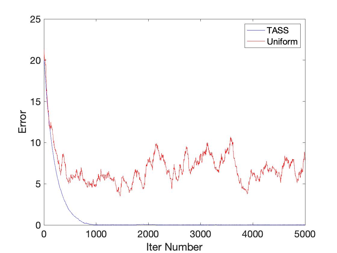
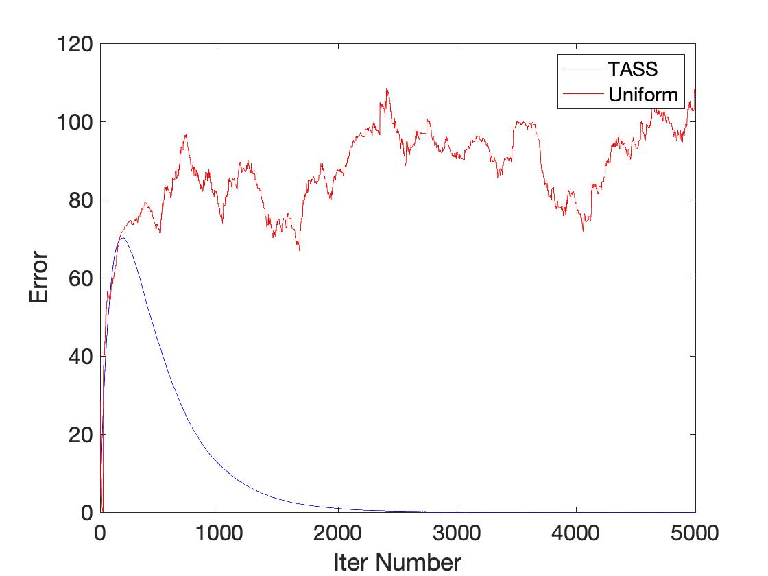
We first compare the performance of rare latent state parameter estimation. In this case, the rare latent state emission parameters are $(\sigma_{3}^{2},\mu_{3})$. We compare $|\sigma_{3}^{2}-\sigma^{2}_{3,\text{true}}|$ and $|\mu_{3}-\mu_{3,\text{true}}|$. The plots are shown in Figure 1. This indicates that TASS converges close to the true parameters in $2\times 10^{3}$ iterations, while uniform sub-sampling appears to have substantial asymptotic (large number of MCMC samples) bias.

Figure 1: Distance between the true and sampled parameter values at different iterations. $|\sigma_{3}^{2}-\sigma^{2}_{3,\text{true}}|$ versus iteration number (left); $|\mu_{3}-\mu_{3,\text{true}}|$ versus iteration number (right).

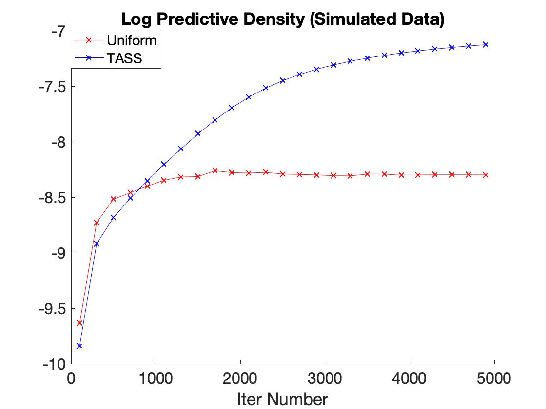
We use predictive performance to compare different sub-sampling algorithms, relying on the expected log predictive density (Gelman et al.,, 2014). We hold out $n_{\text{hold}}=200$ uniformly sampled observations associated with state three without replacement from the test dataset, that is, $\{Y^{(1)},\cdots,Y^{(n_{\text{hold}})}\}\sim\mathrm{Uniform}(\{Y_{t}\mid X_{t}=3\})$. We then estimate the mean log predictive likelihood by

$$\frac{1}{n_{\text{hold}}}\sum_{r=1}^{n_{\text{hold}}}{\rm log}\left(\frac{1}{Z}\sum_{z=1}^{Z}p(Y^{(r)}\mid\theta_{z})\right).$$ (10)

The log-predictive density is plotted in Figure 2. We observe that the log predictive density of TASS is larger than that of the uniform sub-sampling strategy after $10^{3}$ iterations. This indicates that TASS is able to predict rare data more accurately than SGLD with uniform sub-sampling.

Figure 2: Log predictive density of held-out data for one rare latent state example.

4.2 Multiple rare latent states

We consider multiple rare states in this section. We set the transition matrix $A$ to be

$$A=\begin{pmatrix}0.9990&0.1000&0.1000\\ 0.0005&0.9000&0.0000\\ 0.0005&0.0000&0.9000\end{pmatrix}.$$

In this case, the stationary distribution of the latent states is $(0.990,0.005,0.005)^{\top}$ which indicates that both state two and three are rare latent states. We set $\mu=(0,-20,20)^{\top}$ and $\sigma^{2}=(1,1,1)^{\top}$. We simulate $2\times 10^{6}$ observations from the model. We use the first $T=10^{6}$ observations as our training dataset, and the latter $T_{\text{test}}=10^{6}$ observations as our test dataset.

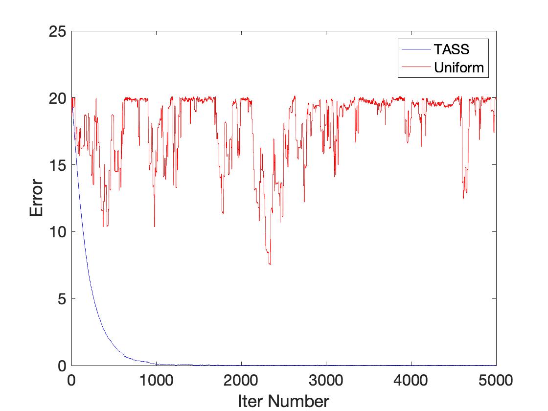
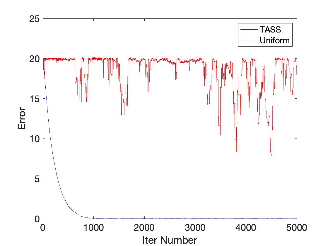
Similar to Section 4.1, we compare the sub-sampling strategies by investigating their respective performance with respect to parameter estimation and predictive performance. To estimate the performance of parameter estimation, we compare $|\mu_{2}-\mu_{2,\text{true}}|$ and $|\mu_{3}-\mu_{3,\text{true}}|$, that is, the distance between emission parameters associated with rare latent states at each iteration to its true value. The results are displayed in Figure 3, which indicates that TASS converges close to the truth in $10^{3}$ iterations, while uniform sub-sampling has substantial asymptotic bias.

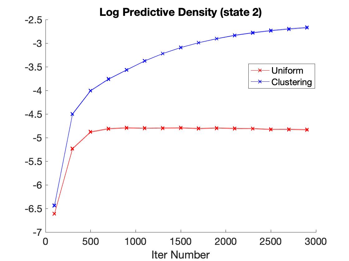
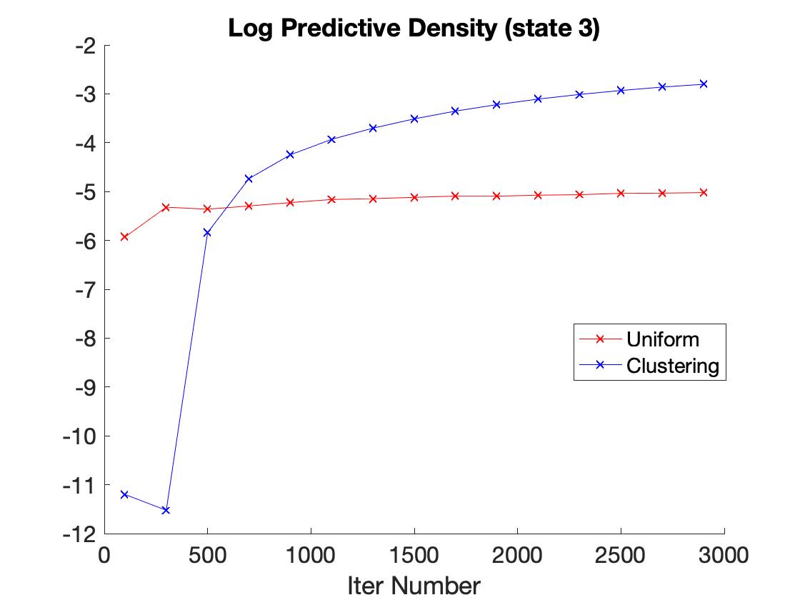
In addition to estimation, we also examine the performance of predicting held-out rare spikes. We uniformly hold out $n_{\text{hold}}=200$ observations each from states two and three in a similar manner as described in the previous section. We then calculate the mean log predictive density as in equation 10. The mean log predictive density versus iteration number is plotted in Figure 4, which again indicates that TASS achieves improved predictive performance relative to uniform sub-sampling at predicting rare states.

Figure 3: Distance between the true and sampled parameter values at different iterations when two rare latent states are presented. $|\mu_{2}-\mu_{2,\text{true}}|$ versus iteration number (left); $|\mu_{3}-\mu_{3,\text{true}}|$ versus iteration number (right).

Figure 4: (Left) Log predictive density of held-out data (state 2) when two rare latent states are present in the dataset. (Right) Log predictive density of held-out data (state 3) when two rare latent states are present in the dataset.

4.3 Run time analysis

We compare the run times of TASS and uniform sub-sampling based SGLD. As compared to uniform sub-sampling, TASS includes an additional clustering and weight calculation step. This additional computational cost is independent of the number of MCMC iterations $n_{\mathrm{MCMC}}$. We consider the same experimental setup as in Section 4.1 with increasing values of $T$ and display CPU run times in Table 2, which shows the additional cost is relatively small.

	$n_{\mathrm{MCMC}}=5\times 10^{3}$		$n_{\mathrm{MCMC}}=6\times 10^{3}$		$n_{\mathrm{MCMC}}=8\times 10^{3}$		$n_{\mathrm{MCMC}}=10^{4}$
	Uniform	TASS	Uniform	TASS	Uniform	TASS	Uniform	TASS
$T=3\times 10^{5}$	190	190	238	245	283	306	353	375
$T=5\times 10^{5}$	249	279	284	323	378	409	492	517
$T=8\times 10^{5}$	330	416	390	483	525	613	638	746
$T=10^{6}$	396	536	476	648	661	845	800	986

Table 2: Run time comparison. All experiments were run on a 2.6 GHz CPU and all run times are CPU times measured in seconds.

5 Application to solar flare data

Solar flares are sudden outbursts of energy from a small area of the sun’s surface. Extreme solar flares can pose a great threat to satellites and thus it is crucial to predict such extreme flares. Solar flares exhibit a normal behavior most of the time with intermittent moments with occasional dangerous spikes. The increasing prevalence of sensor technology has made it possible to attain minute-to-minute data over many days resulting in massively long time series. In analyzing such massive time series, uniform sub-sampling schemes are likely to miss the rare dynamics, thereby hindering prediction and characterization of flare phenomena.

In this section, we consider solar flare X-ray data obtained from the GOES-13 and GOES-15 satellites from September 2017 to April 2018. The dataset consists of $T_{\text{total}}=347875$ time points. Observations are taken from two different satellites, and we average these two different observations prior to our HMM analyses. When one of the satellites is missing an observation at a time point, we simply rely on the other satellites data at that time. Previous work (Stanislavsky et al.,, 2019, 2020) suggests that some hidden switching regimes exist behind the observable X-ray flux.

(a) Raw data.

(b) Preprocessed data.

Figure 5: (a) The raw data. (b) The pre-processed data obtained after subtracting a smooth baseline.

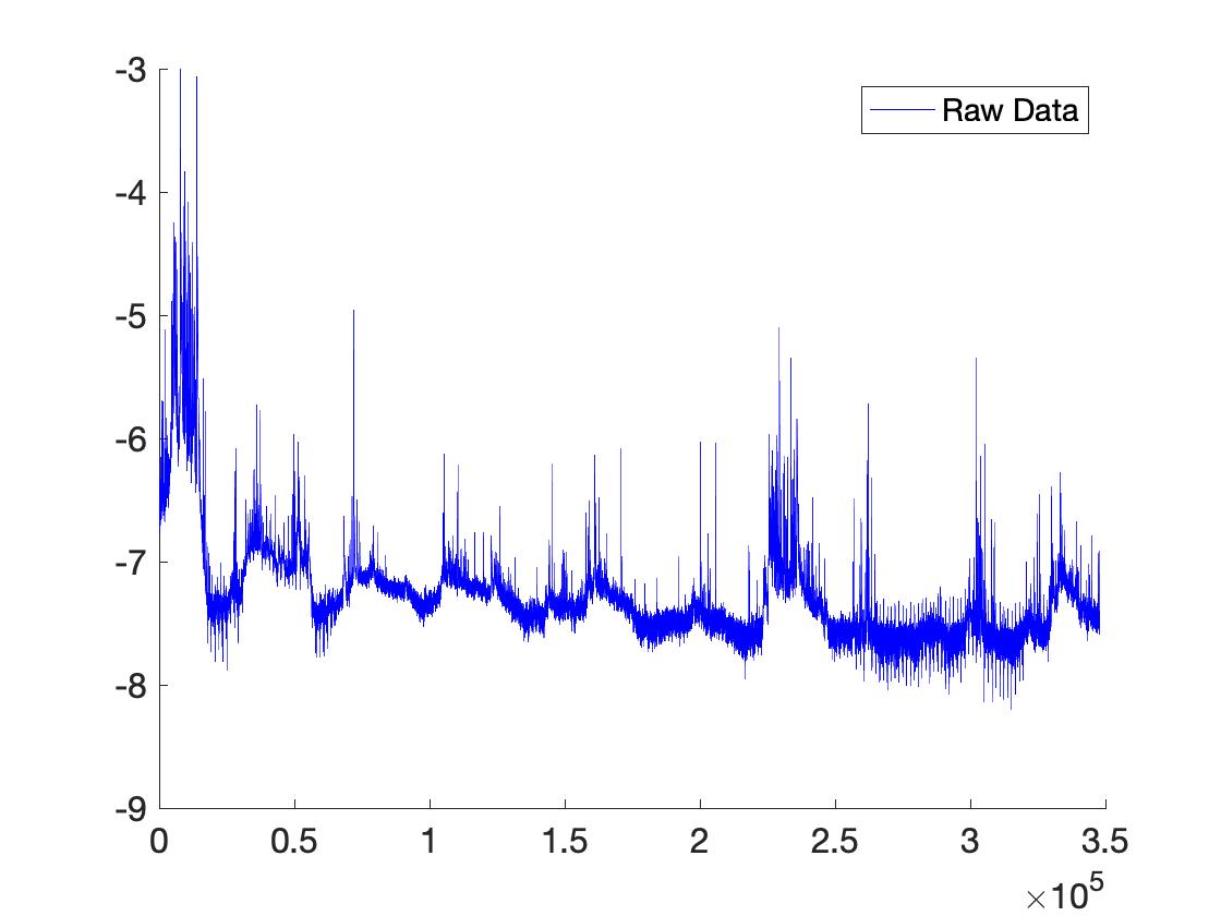
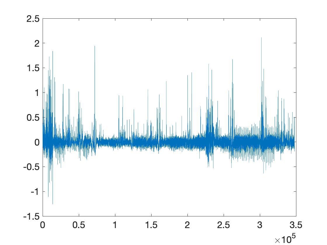
We plot the observed series on the log-scale in Figure 5(a), which clearly suggests that this series is non-stationary. We use a piece-wise quadratic baseline to fit the time trend, and then focus our Bayesian modeling on the residual process after subtracting the baseline. We choose the baseline knots adaptively to adjust for differing volatility at different times. In particular, we place fifty knots evenly in $[1,1.86\times 10^{4}]$, fifty knots in $[1.9\times 10^{4},2.2\times 10^{5}]$, fifty knots in $[2.2\times 10^{5},2.5\times 10^{5}]$, and fifty knots in $[2.5\times 10^{5},T_{\text{total}}]$; the knots are evenly-spaced within each interval. The residual series after baseline subtraction is plotted in Figure 5(b), where we observe occasional rare spikes. Our main objective is to infer the parameters characterizing the rare dynamics and predict the rare spikes. We set $T=3\times 10^{5}$ and use the first $T$ observations as our training dataset and the remaining observations as our test dataset.

Figure 6: Predicted series plots. (top left), (middle left) and (bottom left) are predicted series based on the $4000$th, $4500$th, and $5000$th sample of SGLD using TASS, respectively; (top right), (middle right) and (bottom right) are predicted series based on $4000$th, $4500$th, and $5000$th sample of SGLD with uniform sub-sampling, respectively.

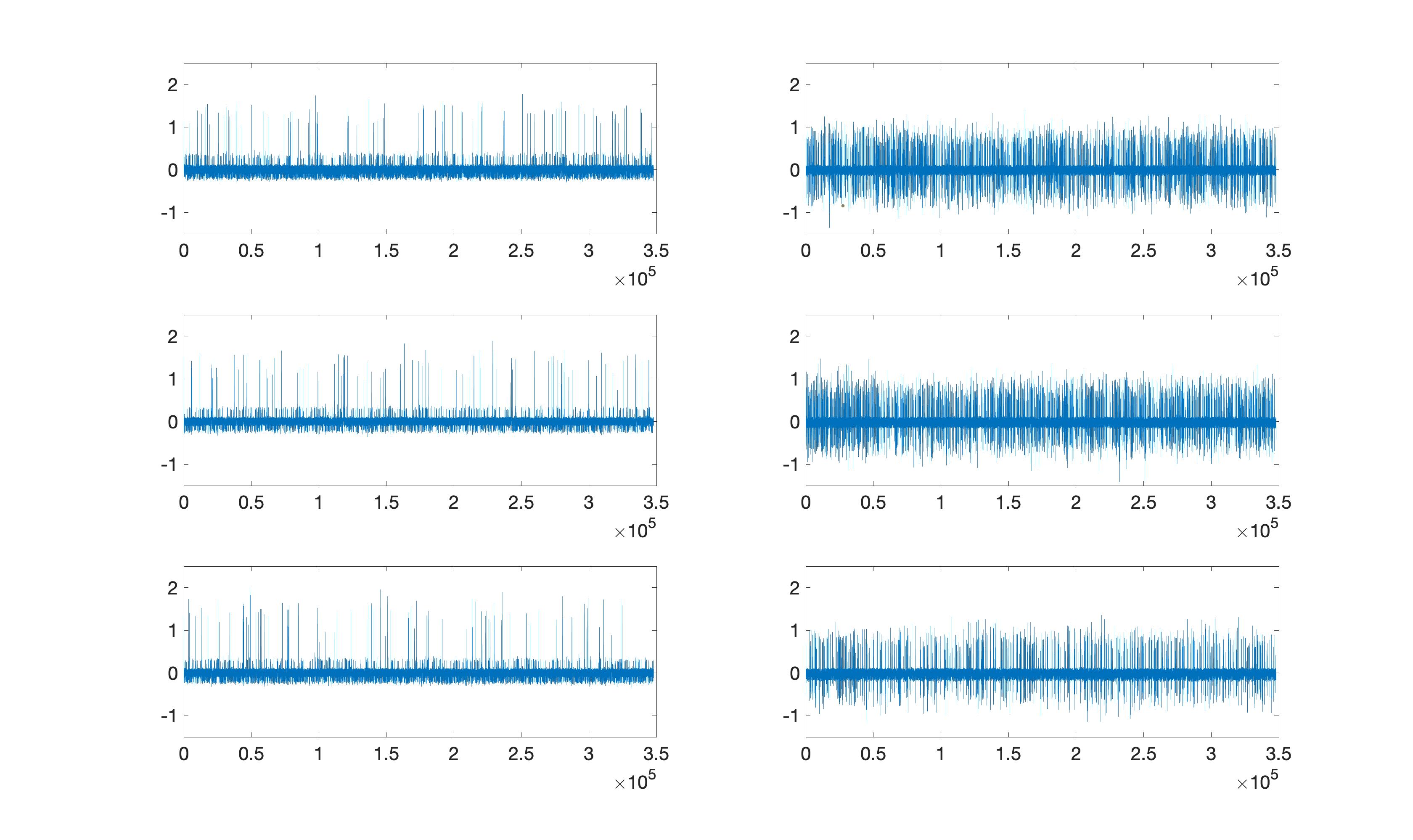
We consider a model with $K=4$ latent states because solar flares can be classified into four categories (Class B, C, M, X) according to their strength as pointed out in Stanislavsky et al., (2020). We assume Gaussian emission distributions and consider the same priors as in Section 4.1. We sub-sample the data by setting half-width $L=2$, sub-sample size $S=10$, and buffer size $B=5$. We run SGLD with for $5\times 10^{3}$ iterations for TASS and uniform sub-sampling. To qualitatively compare the two sub-sampling strategies, we compare the predicted series generated from both samplers, and favor the sampler that renders a predicted series similar to the original data. We plot the predicted series from both samplers based on the $(4000,4500,5000)$th posterior sample, respectively, in Figure 6, and compare them to the original data. We observe that uniform sub-sampling fails to capture the spike behavior, while the predicted series using TASS is able to mimic the rare spikes of the original data. Moreover, the transition rates between the rare latent state and the common states can also be mimicked using TASS.

Figure 7: Log predictive likelihood of the held-out rare spikes of the solar flare dataset.

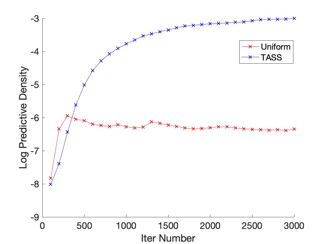
To quantitatively compare the performance of samplers, we set one as the threshold of rare spikes. We identify points that start exceeding this threshold in the test dataset and hold out ten subsequent observations for every point as the held-out dataset. We calculate the predictive likelihood for every held-out subsequence and plot it in Figure 7. We observe that TASS out-performs uniform sub-sampling after approximately $5\times 10^{2}$ iterations with regard to the predictive performance of the rare spike.

6 Discussion

We have proposed a targeted sub-sampling (TASS) approach for stochastic gradient MCMC for discrete state-space hidden Markov models with a particular focus on improving rare latent state inference, which in turn leads to improved predictive performance. We have elected to focus on MCMC algorithms based on Langevin dynamics to simplify the development of the material; however, TASS can be used within stochastic gradient Hamiltonian Monte Carlo (Chen et al.,, 2014) as well. Additional techniques to speed up convergence such as reparameterization and preconditioning can be combined straightforwardly with TASS. While we did not discuss these explicitly, the former was used in estimating the emission parameters using the expanded mean reparameterization of Patterson and Teh, (2013).

Moreover, moving beyond Monte Carlo algorithms, the improved stochastic gradient estimates can be used within any inference scheme for hidden Markov models, including both Bayesian and frequentist approaches. In particular, it can be used within stochastic gradient descent and stochastic variational inference (Foti et al.,, 2014). Furthermore, our coordinate-specific weighting scheme also contributes to the growing body of literature on the advantages of non-uniform data sub-sampling.

Appendix A Proofs

Proof of Proposition 1.

By Condition N of Dalalyan and Karagulyan, (2019), the performance of stochastic-gradient MCMC algorithm is optimized when ${\mathbb{E}}\|\widehat{\nabla}_{\theta}\,\ell(\theta)-\nabla_{\theta}\,\ell(\theta)\|^{2}=\sum_{i=1}^{d}{\mathbb{E}}\{\widehat{\nabla}_{i}\ell(\theta)-\nabla_{i}\,\ell(\theta)\}^{2}$ is minimized. Let $q_{\theta}(Y_{t},x_{t},x_{t-1})={\rm log}\,p_{\theta}(Y_{t}\mid x_{t})+{\rm log}\,p_{\theta}(x_{t}\mid x_{t-1})$. Then

$$\quad\sum_{i=1}^{d}{\mathbb{E}}\{\widehat{\nabla}_{i}\ell(\theta)-\nabla_{i}\ell(\theta)\}^{2}=\sum_{i=1}^{d}\sum_{j=1}^{N}a_{j}\left\{a_{j}^{-1}\sum_{t\in C_{j}}\nabla_{i}\,q_{\theta}(Y_{t},x_{t},x_{t-1})-\nabla_{i}\ell(\theta)\right\}^{2}$$

$$=\sum_{i=1}^{d}\sum_{j=1}^{N}a_{j}\left\{a_{j}^{-1}\sum_{t\in C_{j}}\nabla_{i}\,q_{\theta}(Y_{t},x_{t},x_{t-1})-\nabla_{i}\ell(\theta)\right\}^{2}=\sum_{i=1}^{d}\sum_{j=1}^{N}a_{j}\left\{a_{j}^{-1}\gamma_{ij}(\theta)-\nabla_{i}\ell(\theta)\right\}^{2}$$

for $\gamma_{ij}(\theta)=\sum_{t\in C_{j}}\nabla_{i}\,q_{\theta}(Y_{t},x_{t},x_{t-1})$. Therefore the optimal importance weights are such that

$$\widehat{a}_{1},\dots,\widehat{a}_{N}=\operatorname*{\arg\!\min}_{\begin{subarray}{c}a_{1},\dots,a_{N}:\\ \sum_{j=1}^{N}a_{j}=1\end{subarray}}\sum_{i=1}^{d}\sum_{j=1}^{N}\left\{a_{j}^{-1}\gamma_{ij}^{2}(\theta)+a_{j}\nabla_{i}^{2}\right\}^{2},$$

which can be shown to be the case when

$$\widehat{a}_{j}\propto\sum_{i=1}^{d}\{\gamma_{ij}^{2}(\theta)\}^{1/2}=\left[\sum_{i=1}^{d}\left\{\sum_{t\in C_{j}}\nabla_{i}{\rm log}\,p_{\theta}(Y_{t}\mid x_{t})+\nabla_{i}{\rm log}\,p_{\theta}(x_{t}\mid x_{t-1})\right\}^{2}\right]^{1/2}.\qed$$

The proof of Corollary 1 is very similar to the proof of Proposition 1, with the only difference being that we omit the sum over the components of $\theta$.

References

- Baker et al., (2019) Baker, J., Fearnhead, P., Fox, E. B., and Nemeth, C. (2019). Control variates for stochastic gradient MCMC. Statistics and Computing, 29(3):599–615.
- Baum, (1972) Baum, L. E. (1972). An inequality and associated maximization technique in statistical estimation for probabilistic functions of Markov processes. Inequalities, 3(1):1–8.
- Bierkens et al., (2019) Bierkens, J., Fearnhead, P., and Roberts, G. (2019). The zig-zag process and super-efficient sampling for Bayesian analysis of big data. The Annals of Statistics, 47(3):1288–1320.
- Bishop, (2006) Bishop, C. M. (2006). Pattern Recognition and Machine Learning. Springer.
- Bouchard-Côté et al., (2018) Bouchard-Côté, A., Vollmer, S. J., and Doucet, A. (2018). The bouncy particle sampler: A nonreversible rejection-free Markov chain Monte Carlo method. Journal of the American Statistical Association, 113(522):855–867.
- Campbell and Broderick, (2019) Campbell, T. and Broderick, T. (2019). Automated scalable Bayesian inference via Hilbert coresets. The Journal of Machine Learning Research, 20(1):551–588.
- Chatterji et al., (2018) Chatterji, N., Flammarion, N., Ma, Y., Bartlett, P., and Jordan, M. (2018). On the theory of variance reduction for stochastic gradient Monte Carlo. In International Conference on Machine Learning, pages 764–773. PMLR.
- Chen et al., (2014) Chen, T., Fox, E., and Guestrin, C. (2014). Stochastic gradient Hamiltonian Monte Carlo. In International Conference on Machine Learning, pages 1683–1691. PMLR.
- Csiba and Richtárik, (2018) Csiba, D. and Richtárik, P. (2018). Importance sampling for minibatches. The Journal of Machine Learning Research, 19(1):962–982.
- Dalalyan and Karagulyan, (2019) Dalalyan, A. S. and Karagulyan, A. (2019). User-friendly guarantees for the Langevin Monte Carlo with inaccurate gradient. Stochastic Processes and their Applications, 129(12):5278–5311.
- Duane et al., (1987) Duane, S., Kennedy, A. D., Pendleton, B. J., and Roweth, D. (1987). Hybrid Monte Carlo. Physics Letters B, 195(2):216–222.
- Foti et al., (2014) Foti, N., Xu, J., Laird, D., and Fox, E. (2014). Stochastic variational inference for hidden Markov models. In Advances in Neural Information Processing Systems, pages 3599–3607.
- Fu and Zhang, (2017) Fu, T. and Zhang, Z. (2017). CPSG-MCMC: Clustering-Based Preprocessing method for Stochastic Gradient MCMC. In Singh, A. and Zhu, J., editors, Proceedings of the 20th International Conference on Artificial Intelligence and Statistics, volume 54 of Proceedings of Machine Learning Research, pages 841–850, Fort Lauderdale, FL, USA. PMLR.
- Galagedarage Don and Khan, (2019) Galagedarage Don, M. and Khan, F. (2019). Process fault prognosis using hidden Markov model–Bayesian networks hybrid model. Industrial & Engineering Chemistry Research, 58(27):12041–12053.
- Gelman et al., (2014) Gelman, A., Hwang, J., and Vehtari, A. (2014). Understanding predictive information criteria for Bayesian models. Statistics and Computing, 24(6):997–1016.
- Hall and Willett, (2015) Hall, E. C. and Willett, R. M. (2015). Online convex optimization in dynamic environments. IEEE Journal of Selected Topics in Signal Processing, 9(4):647–662.
- Huggins et al., (2016) Huggins, J., Campbell, T., and Broderick, T. (2016). Coresets for scalable Bayesian logistic regression. In Advances in Neural Information Processing Systems, pages 4080–4088.
- Hughes et al., (2015) Hughes, M. C., Stephenson, W. T., and Sudderth, E. (2015). Scalable adaptation of state complexity for nonparametric hidden Markov models. In Advances in Neural Information Processing Systems, pages 1198–1206.
- Hunt and Willett, (2018) Hunt, X. J. and Willett, R. (2018). Online data thinning via multi-subspace tracking. IEEE Transactions on Pattern Analysis and Machine Intelligence, 41(5):1173–1187.
- Johnson and Willsky, (2014) Johnson, M. and Willsky, A. (2014). Stochastic variational inference for Bayesian time series models. In International Conference on Machine Learning, pages 1854–1862. PMLR.
- Johnson, (2014) Johnson, M. J. (2014). Bayesian time series models and scalable inference. PhD thesis, Massachusetts Institute of Technology.
- Johnson and Guestrin, (2018) Johnson, T. B. and Guestrin, C. (2018). Training deep models faster with robust, approximate importance sampling. Advances in Neural Information Processing Systems, 31:7265–7275.
- Juang and Rabiner, (1990) Juang, B. . and Rabiner, L. R. (1990). The segmental k-means algorithm for estimating parameters of hidden Markov models. IEEE Transactions on Acoustics, Speech, and Signal Processing, 38(9):1639–1641.
- Kerdprasop and Kerdprasop, (2010) Kerdprasop, K. and Kerdprasop, N. (2010). Parallelization of k-means clustering on multi-core processors. In Proceedings of the 10th WSEAS International Conference on Applied Computer Science, volume 10, pages 472–477.
- Kraj et al., (2008) Kraj, P., Sharma, A., Garge, N., Podolsky, R., and McIndoe, R. A. (2008). Parakmeans: Implementation of a parallelized k-means algorithm suitable for general laboratory use. BMC Bioinformatics, 9(1):1–13.
- Ma et al., (2017) Ma, Y.-A., Foti, N. J., and Fox, E. B. (2017). Stochastic gradient MCMC methods for hidden Markov models. In International Conference on Machine Learning, pages 2265–2274. PMLR.
- Muhammad et al., (2018) Muhammad, H. Z., Nasrun, M., Setianingsih, C., and Murti, M. A. (2018). Speech recognition for English to Indonesian translator using hidden Markov model. In 2018 International Conference on Signals and Systems (ICSigSys), pages 255–260. IEEE.
- Needell et al., (2014) Needell, D., Ward, R., and Srebro, N. (2014). Stochastic gradient descent, weighted sampling, and the randomized kaczmarz algorithm. In Ghahramani, Z., Welling, M., Cortes, C., Lawrence, N., and Weinberger, K. Q., editors, Advances in Neural Information Processing Systems, volume 27. Curran Associates, Inc.
- Ourston et al., (2003) Ourston, D., Matzner, S., Stump, W., and Hopkins, B. (2003). Applications of hidden Markov models to detecting multi-stage network attacks. In 36th Annual Hawaii International Conference on System Sciences, 2003. Proceedings of the, pages 10–pp. IEEE.
- Patterson and Teh, (2013) Patterson, S. and Teh, Y. W. (2013). Stochastic gradient Riemannian Langevin dynamics on the probability simplex. In NIPS, pages 3102–3110.
- Petropoulos et al., (2016) Petropoulos, A., Chatzis, S. P., and Xanthopoulos, S. (2016). A novel corporate credit rating system based on student’s-t hidden Markov models. Expert Systems with Applications, 53:87–105.
- Peyravi et al., (2019) Peyravi, F., Latif, A., and Moshtaghioun, S. M. (2019). A composite approach to protein tertiary structure prediction: hidden Markov model based on lattice. Bulletin of Mathematical Biology, 81(3):899–918.
- Quiroz et al., (2019) Quiroz, M., Kohn, R., Villani, M., and Tran, M.-N. (2019). Speeding up MCMC by efficient data subsampling. Journal of the American Statistical Association, 114(526):831–843.
- Raginsky et al., (2017) Raginsky, M., Rakhlin, A., and Telgarsky, M. (2017). Non-convex learning via stochastic gradient langevin dynamics: a nonasymptotic analysis. In Conference on Learning Theory, pages 1674–1703. PMLR.
- Roberts and Tweedie, (1996) Roberts, G. O. and Tweedie, R. L. (1996). Exponential convergence of Langevin distributions and their discrete approximations. Bernoulli, 2(4):341–363.
- Salomone et al., (2020) Salomone, R., Quiroz, M., Kohn, R., Villani, M., and Tran, M.-N. (2020). Spectral subsampling MCMC for stationary time series. In International Conference on Machine Learning, pages 8449–8458. PMLR.
- Scott, (2002) Scott, S. L. (2002). Bayesian methods for hidden Markov models: Recursive computing in the 21st century. Journal of the American Statistical Association, 97(457):337–351.
- Sen et al., (2020) Sen, D., Sachs, M., Lu, J., and Dunson, D. B. (2020). Efficient posterior sampling for high-dimensional imbalanced logistic regression. Biometrika, 107(4):1005–1012.
- Stanislavsky et al., (2020) Stanislavsky, A., Nitka, W., Małek, M., Burnecki, K., and Janczura, J. (2020). Prediction performance of hidden Markov modelling for solar flares. Journal of Atmospheric and Solar-Terrestrial Physics, 208:105407.
- Stanislavsky et al., (2019) Stanislavsky, A. A., Burnecki, K., Janczura, J., Niczyj, K., and Weron, A. (2019). Solar X-ray variability in terms of a fractional heteroskedastic time series model. Monthly Notices of the Royal Astronomical Society, 485(3):3970–3980.
- Volant et al., (2014) Volant, S., Bérard, C., Martin-Magniette, M.-L., and Robin, S. (2014). Hidden Markov models with mixtures as emission distributions. Statistics and Computing, 24(4):493–504.
- Welling and Teh, (2011) Welling, M. and Teh, Y. W. (2011). Bayesian learning via stochastic gradient Langevin dynamics. In Proceedings of the 28th International Conference on Machine Learning (ICML-11), pages 681–688. Citeseer.
- Zhang et al., (2019) Zhang, X., Li, Y., Wang, S., Fang, B., and Philip, S. Y. (2019). Enhancing stock market prediction with extended coupled hidden Markov model over multi-sourced data. Knowledge and Information Systems, 61(2):1071–1090.
- Zou et al., (2018) Zou, D., Xu, P., and Gu, Q. (2018). Subsampled stochastic variance-reduced gradient Langevin dynamics. In International Conference on Uncertainty in Artificial Intelligence.
- Zou et al., (2020) Zou, D., Xu, P., and Gu, Q. (2020). Faster convergence of stochastic gradient langevin dynamics for non-log-concave sampling. arXiv preprint arXiv:2010.09597.