The Statistical Model of Nuclear Reactions: Open Problems

Abstract

Several experiments [1, 2, 3] show significant deviations from predictions of the statistical model of nuclear reactions. We summarize unsuccessful recent theoretical efforts to account for such disagreement in terms of a violation of orthogonal invariance caused by the Thomas-Ehrman shift. We report on numerical simulations involving a large number of gamma decay channels that also give rise to violation of orthogonal invariance but likewise do not account for the discrepancies. We discuss the statistical model in the light of these results.

0.1 Motivation

In recent years, several predictions of the statistical model of nuclear reactions have been tested experimentally, with puzzling results. The statistical model predicts that the reduced partial neutron widths of isolated compound-nucleus resonances have a Porter-Thomas distribution (PTD), i.e., a $\chi^{2}$ distribution in one degree of freedom. Moreover, the total gamma decay width of an isolated neutron resonance is the sum of a very large number of partial gamma decay widths. If the latter have a PTD, the distribution of total gamma decay widths should be very narrow. However, the data show strong deviations from these predictions:

(i) In the scattering of slow neutrons on the target nuclei ¹⁹²Pt and ¹⁹⁴Pt, 158 and 411 isolated resonances, respectively, were analysed. The data reject the validity of the PTD with $99.997\%$ statistical significance [1].

(ii) A reanalysis of the nuclear data ensemble (NDE) rejects the validity of the PTD with $99.97\%$ statistical significance [2].

(iii) The measured distributions of total gamma decay widths for isolated neutron resonances in the compound nucleus ⁹⁶Mo are much wider and are peaked at significantly larger values of the widths than predicted by the statistical model. The ground state of the nucleus ⁹⁵Mo has spin/parity $5/2^{+}$, hence $s$-wave and $p$-wave resonances in the compound nucleus ⁹⁶Mo have spin/parity values $2^{+},3^{+}$ and $1^{-},2^{-},3^{-},4^{-}$, respectively. For all these spin/parity values, Fig. 1 shows the measured cumulative width distributions (i.e., the fraction of widths larger than a given value) as dark lines with error bars and the values predicted by the statistical model as red lines [3].

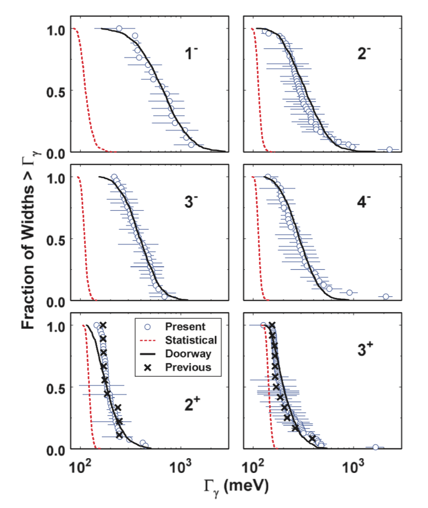
Figure 1: Cumulative distributions of the total gamma decay widths for neutron resonances in ⁹⁶Mo as described in the text. Taken from Ref. [3].

Here we summarize previous attempts and present a new approach aimed at reconciling the statistical model with the data of Refs. [1, 2, 3]. To that end, we first recall in Sec. 0.2 the essential features of the statistical model.

0.2 Statistical Model

For states of fixed spin and parity, we consider a compound-nucleus (CN) reaction induced by slow neutrons ($s$-wave or $p$-wave) that leads either to elastic neutron scattering or to gamma decay of the CN. We neglect direct reactions. Denoting by $c=1$ the neutron channel and $c=2,3,\ldots,\Lambda\gg 1$ the gamma channels, the scattering matrix is

$$S_{cc^{\prime}}(E)=\delta_{cc^{\prime}}-2i\pi\sum_{\mu\nu}W_{c\mu}(E)[(E-H^{\rm eff})^{-1}]_{\mu\nu}W_{\nu c^{\prime}}(E)\;.$$ (1)

Here $E$ is the excitation energy of the CN, with $E=0$ for the ground state. The threshold energy of channel $c$ is denoted by $E_{c}$. The real matrix elements $W_{c\mu}(E)=W_{\mu c}(E)$ (defined for $E\geq E_{c}$) describe the coupling of channel $c$ to the compound nucleus states, spanned by the states $\mu=1,2,\ldots,N\gg 1$. In the framework of the statistical model, the nuclear Hamiltonian is, within the space of compound states, replaced by $H^{\rm GOE}$, a matrix of dimension $N\gg 1$ drawn from the Gaussian orthogonal ensemble (GOE) of random matrices [4]. The effective Hamiltonian is given by

$$H^{\rm eff}_{\mu\nu}=H^{\rm GOE}_{\mu\nu}+\sum_{c}{\cal P}\int_{E_{c}}^{\infty}{\rm d}E^{\prime}\ \frac{W_{\mu c}(E^{\prime})W_{c\nu}(E^{\prime})}{E-E^{\prime}}-i\pi\sum_{c}W_{\mu c}(E)W_{c\nu}(E)\;,$$ (2)

where $\cal P$ denotes the principal-value integral.

The derivation of the PTD rests on the fact that the GOE is invariant under orthogonal transformations in the space of compound states. Such invariance is violated by the last two terms on the right-hand side of Eq. (2), describing the coupling of the CN to the channels. In recent years, considerable theoretical effort has been devoted to the question whether the discrepancies listed in Sec. 0.1 can be attributed to these two terms.

We discuss these terms using simplifications that apply in the present case. (i) For the overwhelming majority of gamma channels ($c\geq 2$) the gamma decay energy $E$ differs substantially from the threshold energy $E_{c}$. Then it is legitimate to neglect the principal-value integrals, and we do so for all gamma channels. (ii) For slow neutrons the energy dependence of the matrix elements that couple to the neutron channel is given by $W_{1\mu}(E)\approx(E-E_{1})^{(2l+1)/4}W^{(0)}_{1\mu}$. Here $l=0$ ($l=1$) for $s$-wave ($p$-wave) neutrons, respectively, while $W^{(0)}_{1\mu}$ is independent of energy. With that approximation the two coupling terms in Eq. (2) are given by the product of $W^{(0)}_{\mu 1}W^{(0)}_{1\nu}$ and of a complex energy-dependent factor that is independent of $\mu,\nu$. (iii) The absence of direct reactions implies channel orthogonality in the form $\pi\sum_{\mu}W_{c\mu}W_{\mu c^{\prime}}=\delta_{cc^{\prime}}\lambda\kappa_{c}$. Here $\lambda=Nd/\pi$ is the standard GOE parameter and $d$ is the mean GOE level spacing in the center of the spectrum. The dimensionless parameter $\kappa_{c}$ measures the strength of the coupling to channel $c$. Channel orthogonality allows us to diagonalize the matrices coupling the compound states to the channels, and we obtain

$$H^{\rm eff}_{\mu\nu}=H^{\rm GOE}_{\mu\nu}+\delta_{\mu\nu}V_{\mu}\ ,$$ (3)

where

$$V_{c}=\left\{\begin{array}[]{cl}\lambda\bigg{(}\frac{1}{\pi}{\cal P}\int_{E_{1}}^{\infty}{\rm d}E^{\prime}\frac{\kappa_{1}(E^{\prime})}{E-E^{\prime}}-i\kappa_{1}(E)\bigg{)}&{\rm for}\ c=1\;,\\ -i\lambda\kappa_{c}&{\rm for}\ c=2,\ldots,\Lambda\;,\\ 0&{\rm for}\ c>\Lambda\;.\end{array}\right.$$ (7)

The average $S$ matrix is $\langle S_{cc^{\prime}}\rangle=\delta_{cc^{\prime}}(1-\kappa_{c})/(1+\kappa_{c})$, and the transmission coefficient in channel $c$ is $T_{c}=1-|\langle S_{cc}\rangle|^{2}=4\kappa_{c}/(1+\kappa_{c})^{2}$.

0.3 Nonstatistical Effects: Thomas-Ehrman Shift

In the platinum isotopes, the single-particle $4s$ state of the nuclear shell model is close to neutron threshold, causing a maximum of the $s$-wave neutron strength function in that mass region and, at the same time, an enhancement of the principal-value integral (the shift function) in $V_{1}$ of Eq. (7). In light nuclei the shift due to the principal-value integral is known as the Thomas-Ehrman shift. Several authors [5, 6, 7] have addressed the question whether that enhancement may be responsible for deviations of the distribution of partial neutron resonance widths from the PTD. In all these works, the gamma channels were neglected (except for a constant imaginary shift in the GOE energies).

For real values of $V_{1}$ that are consistent with the enhancement due to the $4s$ state but were taken to be independent of energy, the numerical results of Volya et al. [5] showed significant deviations of the distribution of reduced partial neutron widths from the PTD. Bogomolny [6] succeeded in diagonalizing the Hamiltonian (3) with an energy-independent real $V_{1}$ in the limit of large matrix dimension $N$. He showed that deviations from the PTD do arise but that locally the width distribution remains a PTD. The effect found in Ref. [5] is attributed to ignoring the secular variation of the average width with energy. Once the average width is divided out, the fluctuations of the reduced widths follow the PTD. Fanto et. al. [7] studied a model that includes a realistic description of the neutron channel in a Woods-Saxon potential, and effectively takes full account of the energy dependence of $V_{1}$. The resulting local distribution of partial neutron widths was found to be consistent with the PTD.

We note that a sufficiently large imaginary part of $V_{1}$ can lead to deviations from a PTD [8]. However, no such deviations are observed for realistic values of $\kappa_{1}$ [5, 7].

Therefore, the deviations from the PTD listed under (i) and (ii) in Sec. 0.1 cannot, for realistic values of the parameters, be accounted for by violations of orthogonal invariance due to the coupling to the neutron channel. In view of this result, we consider the shift function in the first of Eqs. (7) to be insignificant and we disregard it in what follows.

0.4 Nonstatistical Effects: Many Gamma Channels

In medium-mass and heavy nuclei, the number of gamma decay channels is huge (of the order of $10^{6}$ or so) for each isolated neutron resonance. We ask: can that fact account for the deviations listed in Sec. 0.1 even though the coupling of each individual gamma channel to the CN is very weak? Prior to addressing that question we recall in Sec. 0.4.1 the calculation of the total gamma decay width in the statistical model.

0.4.1 Total Gamma Width

An isolated neutron resonance labelled $\mu$ with spin/parity $J^{\pi}$ and resonance energy $E_{\mu}$ decays by emission of photons of multipolarity $L$ and parity $\pi$ (E1, M1, E2, M2, …, jointly written as $XL$) to final states $f$ with spins/parities $J^{\pi}_{f}$. (The label $f$ replaces the channel label $c$ used in Eq. (3).) The corresponding partial decay widths are denoted by $\Gamma^{J^{\pi}}_{\mu\gamma J^{\pi}_{f}fXL}$. The total gamma decay width is

$$\Gamma^{J^{\pi}}_{\mu\gamma}=\sum_{XL}\sum_{J^{\pi}_{f}f}\Gamma^{J^{\pi}}_{\mu\gamma J^{\pi}_{f}fXL}\ .$$ (8)

In the statistical model, the partial width is written as a product,

$$\Gamma^{J^{\pi}}_{\mu\gamma I^{\pi}_{f}fXL}=x^{2}_{f}\langle\Gamma^{J^{\pi}}_{\mu\gamma J^{\pi}_{f}fXL}\rangle\ .$$ (9)

The average value in Eq. (9) is expressed in terms of the gamma strength function $f_{XL}(E_{\gamma})$ and the average spacing $d_{J^{\pi}}$ of the resonances of spin $J$ and parity $\pi$,

$$\langle\Gamma^{J^{\pi}}_{\mu\gamma I^{\pi}_{f}fXL}\rangle=d_{J^{\pi}}E^{2L+1}_{\gamma}f_{XL}(E_{\gamma})=d_{J^{\pi}}\frac{2}{\pi}\kappa_{f}\;,$$ (10)

where the dimensionless parameters $\kappa_{f}$ have the same physical meaning as the parameters $\kappa_{c}$ in Eq. (7). The factors $x^{2}_{f}$ are uncorrelated random variables that each have mean value unity and follow the PTD. These account for fluctuations of the partial widths. The statistical model is implemented by choosing values for the strength function and for the average level density from which the actual values of the final energies $E_{f}$ are drawn. The average total total gamma decay width is given by

$$\langle\Gamma^{J^{\pi}}_{\mu\gamma}\rangle=d_{J^{\pi}}\sum_{XL}\sum_{J^{\pi}_{f}}\int_{0}^{E_{\mu}}{\rm d}E_{\gamma}\ \rho(E_{\mu}-E_{\gamma},J^{\pi}_{f})E^{2L+1}_{\gamma}f_{XL}(E_{\gamma})\;,$$ (11)

where $\rho(E_{\mu}-E_{\gamma},J^{\pi}_{f})$ is the average level density at energy $E_{\mu}-E_{\gamma}$ and spin/parity $J^{\pi}_{f}$ of the final levels into which the compound nucleus decays.

0.4.2 Simulation of Gamma Decay of the ⁹⁶Mo Compound Nucleus

The influence of the coupling of many gamma channels on the statistical properties of the neutron resonances was simulated as follows. It is impractical to use in Eqs. (3) and (7) the totality of channels $f$ resulting from the treatment in Section 0.4.1. Their number is simply too large. For each group of neutron resonances carrying spin-parity values $(2^{+},3^{+})$ for $s$-wave neutrons and $(1^{-},2^{-},3^{-},4^{-})$ for $p$-wave neutrons, a set of representative channels $c=1,2,\ldots,\Lambda-1$ (distinguished in notation from the actual channels labelled $f$) was constructed instead. Below an excitation energy of $2.79$ MeV, known measured discrete levels were used. Above that energy, representative channels labelled $c$ were defined by coarse-graining: final states $f$ close in energy and carrying identical quantum numbers were grouped together. The average density of final states $c$ was taken proportional to the actual level density. For the latter, the back-shifted Fermi gas model with a spin distribution described by the spin cutoff model were used. States with opposite parity were assumed to have the same level density. Only E1 and M1 gamma transitions were considered as these contribute the bulk to the widths. For the E1 and M1 strength functions the parametrization of Ref. [9] was used. The effective coupling parameters $\kappa_{c}$ are sums over the parameters $\kappa_{f}$ for the states $f$ in the group. The number of gamma channels so constructed was $400$. The total number of channels was 401: one neutron channel, 200 E1 channels, and 200 M1 channels. Results shown below are taken from the middle of the GOE spectrum to avoid edge effects.

0.4.3 Results

The scheme described in Sec. 0.4.2 was used to check for deviations of neutron and gamma decay widths from the PTD. For a width $\Gamma$ and its average $\langle\Gamma\rangle$ we define $x=\Gamma/\langle\Gamma\rangle$ and $y=\ln x$. For $y$ the PTD takes the form $P(y)=\sqrt{x/(2\pi)}\exp(-x/2)$. For neutron resonances with spin/parity $2^{+}$ that function is shown in Fig. 2 for the partial widths in the neutron channel and in the most strongly coupled E1 channel. The solid black lines describe the PTD, and the histograms are the result of the simulations. They agree perfectly. We have found similar agreement for less strongly coupled gamma channels and for other spin/parity values. We conclude that a large number of gamma channels with realistic coupling strengths does not alter the PTD of partial widths in any channel (neutron or gamma).

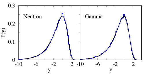
Figure 2: Distribution of $y=\ln x$, where $x=\Gamma/\langle\Gamma\rangle$ is the reduced partial width. The left panel shows the result for the neutron channel, the right panel shows the result for the most strongly coupled gamma channel. Histograms are model calculations (see text), and the solid black lines are the PTD.

Total gamma decay widths were obtained from Eqs. (8), (9) and (10) with the adopted values for the level density and the strength function, and with a PTD for the variables $x^{2}_{f}$. To check for the sensitivity of our results to the form of the strength function we have used three different parametrizations of the E1 strength function displayed in Fig. 3. The blue solid line describes the standard parameterization of the E1 strength function, the red dotted-dashed line is found by taking twice the width of the giant dipole resonance in the E1 strength function, and the green dashed line corresponds to half the width of the giant dipole resonance. The resulting cumulative distributions of the total gamma decay width for the $2^{+}$ neutron resonances (normalized to give the experimental total average gamma width) are shown in Fig. 4. These cumulative distributions virtually coincide. Also shown with error bars is the measured cumulative distribution of Ref. [3]. That distribution is clearly much wider than the simulated ones.

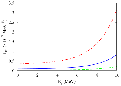
Figure 3: Three different parametrizations of the E1 strength function as described in the text.

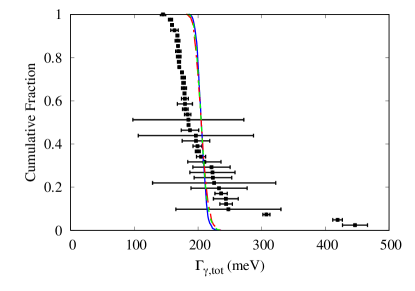
Figure 4: The cumulative distribution of the total gamma decay width for the $2^{+}$ resonances in ⁹⁶Mo. The black squares with error bars are data taken from Ref. [3]. The three colored lines correspond to simulations that use the three parametrizations of the E1 strength function shown in Fig. 3.

The disagreement of statistical-model predictions with the data of Ref. [3] extends to the maxima of the (un-normalized) total gamma decay width distributions. Table 1 shows that the locations of the peaks of the distributions (or more accurately, the average values) also differ markedly. The experimental average total widths have significantly larger values than the corresponding average withs predicted by the statistical model. For the $1^{-}$ states the ratio is larger than three. Individual peak positions for given spin/parity can be fitted by an ad-hoc modification of the E1 strength function. It was not possible, however, to fit all peak positions simultaneously by such modification.

$J^{\pi}$	$2^{+}$	$3^{+}$	$1^{-}$	$2^{-}$	$3^{-}$	$4^{-}$
$\langle\Gamma_{\gamma,\rm sim}\rangle$ (meV)	165.5	157.5	191.2	172.8	169.2	153.8
$\langle\Gamma_{\gamma,\rm exp}\rangle$ (meV)	206 (31)	240 (58)	670 (225)	374 (115)	404 (100)	361 (106)

Table 1: Comparison of simulated average total gamma widths $\langle\Gamma_{\gamma,\rm sim}\rangle$ with the experimental results $\langle\Gamma_{\gamma,\rm exp}\rangle$.

The PTD for the partial gamma decay widths is corroborated by the results shown in Fig. 2. The disagreement of the simulated neutron partial width distribution (a PTD) with the data of Refs. [1, 2] may cast doubt on the validity of that conclusion. That raises the question: Would a distribution of partial gamma widths different from the PTD yield better agreement of the predicted distribution of total gamma widths with the data of Ref. [3]? To generate such a distribution we have used a dynamical model with an unrealistically strong coupling of the GOE Hamiltonian to the neutron channel, $V_{\mu}=-i0.8\lambda\delta_{\mu 1}$ in Eq. (3). The resulting distributions of the partial widths are shown in Fig. 5 for the neutron channel (blue histograms) and for one gamma channel (green histograms). Both distributions differ markedly from the PTD (black). It is noteworthy that strong coupling to the neutron channel also modifies the width distribution in the gamma channels. However, Fig. 6 shows that use of the modified distribution for the gamma channels does not affect the disagreement with the data of Ref. [3]. The calculated cumulative distribution for the $2^{+}$ resonances using the modified gamma channel distribution (dashed green line) is nearly indistinguishable from the one obtained using the PTD (black line). Even if we use for the partial gamma width distribution the blue distribution in Fig. 5 (i.e., assuming the gamma channels to be strongly coupled to the resonances), the resulting cumulative distribution (dashed-dotted blue line) is not much different. In comparison, the data for the $2^{+}$ resonances (black squares with error bars) differ substantially from the theoretical curves.

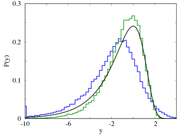
Figure 5: Distribution of $y_{i}=\ln x_{i}$ for the model of Eq. (3) with $V_{\mu}=-i0.8\lambda\delta_{\mu 1}$, where $i=1$ denotes the neutron channel (blue histogram) and $i=2$ denotes one gamma channel (green histogram). The set $\{x_{i}\}$ equals the set $\{\Gamma_{i\mu}/\langle\Gamma_{i\mu}\rangle)\}$, and $y_{i}=\ln x_{i}$ as in Fig. 2. The solid black line is the PTD.

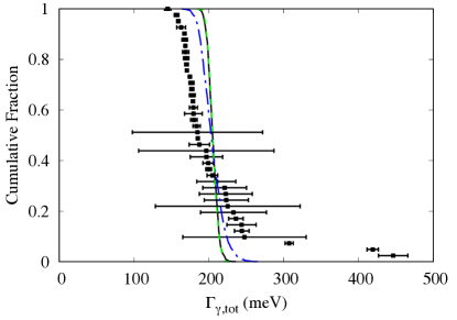
Figure 6: Simulated cumulative total width distributions are compared with experimental data for resonances of spin-parity $2^{+}$. The black solid line is obtained using the PTD for the partial widths. The green dashed line and blue dotted-dashed line are obtained using modified distributions for the partial gamma widths given, respectively, by the green and blue histograms in Fig. 5. The black squares with error bars show the experimental data of Ref. [3]. The simulated widths are normalized to match the experimental average total width.

The reason for the near coincidence of the simulated cumulative distributions is actually quite simple. According to the construction in Eqs. (8) to (9), the total gamma width is the sum of a very large number ($K$, say) of independently distributed random variables with similar or identical distributions (describing the partial gamma widths). The central limit theorem implies that the total width has a Gaussian distribution with a variance that is inversely proportional to $K$. The narrowness of the predicted total width distributions is, thus, independent of the actual form of the partial-width distribution and is a universal feature resulting directly from the basic tenets of the statistical model.

0.5 Discussion

The distributions of reduced partial neutron widths reported in Refs. [1, 2] deviate significantly from the PTD. Within the framework of the statistical model, violation of orthogonal invariance is a possible culprit. Two mechanisms for such violation have been investigated. The Thomas-Ehrman shift, addressed by several authors, is ruled out. Simulations involving a large number of gamma channels yield perfect agreement with the PTD in all channels. That mechanism is, therefore, also ruled out. Furthermore, the measured distributions of total gamma decay widths in ⁹⁶Mo reported in Ref. [3] disagree with those obtained in simulations that follow the statistical model. These predicted distributions are too narrow, and the mean values of the total gamma widths are too small when compared with the experimental results.

In summary, the statistical model fails to account for the data in platinum isotopes, in the nuclear data ensemble, and in ⁹⁶Mo. Violation of orthogonal invariance due to channel coupling cannot be held responsible for these failures. The observed deviations suggest that at neutron threshold, the mixing of CN states is less complete than implied in the statistical model by the use of a GOE Hamiltonian. The small mean values of the total gamma decay widths predicted by the statistical model show that gamma strength is missing in the model. That poses the question whether the Brink-Axel hypothesis actually applies to all gamma transitions that contribute significantly to the gamma decay of the neutron resonances. Such consequences are rather drastic. We feel that additional experimental tests of the statistical model are called for.

Given the experimental results, a small number of strong gamma transitions to low-lying final states might offer a way out of the dilemma [3]. These should have sufficient intensity to shift the simulated distribution of total gamma decay widths towards the experimental values. Their number should be sufficiently small to overcome the limits of the central-limit theorem and to broaden the distribution of total gamma decay widths. It is an open question whether a comparatively small number of such strongly coupled gamma decay channels could also cause a change of the PTD for the reduced neutron widths.

References

- [1] P. E. Koehler et al., Phys. Rev. Lett. 105, 072502 (2010).
- [2] P. E. Koehler, Phys. Rev. C 84, 034312 (2011).
- [3] P. E. Koehler, Phys. Rev. C 88, 041305(R) (2013).
- [4] G. E. Mitchell, A. Richter, and H. A. Weidenmüller, Rev. Mod. Phys. 82, 2845 (2010).
- [5] A. Volya, H. A. Weidenmüller, and V. Zelevinsky, Phys. Rev. Lett. 115, 052501 (2015).
- [6] E. Bogomolny, Phys. Rev. Lett. 118, 022501 (2017).
- [7] P. Fanto, G. F. Bertsch, and Y. Alhassid, Phys. Rev. C 98, 014604 (2018).
- [8] G. L. Celardo, N. Auerbach, F. M. Izrailev, and V. G. Zelevinsky, Phys. Rev. Lett. 106, 042501 (2011).
- [9] S. A. Sheets, Phys. Rev. C 79, 024301 (2009).