On Fast Leverage Score Sampling and Optimal Learning

Abstract

Leverage score sampling provides an appealing way to perform approximate computations for large matrices. Indeed, it allows to derive faithful approximations with a complexity adapted to the problem at hand. Yet, performing leverage scores sampling is a challenge in its own right requiring further approximations. In this paper, we study the problem of leverage score sampling for positive definite matrices defined by a kernel. Our contribution is twofold. First we provide a novel algorithm for leverage score sampling and second, we exploit the proposed method in statistical learning by deriving a novel solver for kernel ridge regression. Our main technical contribution is showing that the proposed algorithms are currently the most efficient and accurate for these problems.

1 Introduction

A variety of machine learning problems require manipulating and performing computations with large matrices that often do not fit memory. In practice, randomized techniques are often employed to reduce the computational burden. Examples include stochastic approximations [1], columns/rows subsampling and more general sketching techniques [2, 3]. One of the simplest approach is uniform column sampling [4, 5], that is replacing the original matrix with a subset of columns chosen uniformly at random. This approach is fast to compute, but the number of columns needed for a prescribed approximation accuracy does not take advantage of the possible low rank structure of the matrix at hand. As discussed in [6], leverage score sampling provides a way to tackle this shortcoming. Here columns are sampled proportionally to suitable weights, called leverage scores (LS) [7, 6]. With this sampling strategy, the number of columns needed for a prescribed accuracy is governed by the so called effective dimension which is a natural extension of the notion of rank. Despite these nice properties, performing leverage score sampling provides a challenge in its own right, since it has complexity in the same order of an eigendecomposition of the original matrix. Indeed, much effort has been recently devoted to derive fast and provably accurate algorithms for approximate leverage score sampling [2, 8, 6, 9, 10].
In this paper, we consider these questions in the case of positive semi-definite matrices, central for example in Gaussian processes [11] and kernel methods [12]. Sampling approaches in this context are related to the so called Nyström approximation [13] and Nyström centers selection problem [11], and are widely studied both in practice [4] and in theory [5]. Our contribution is twofold. First, we propose and study BLESS, a novel algorithm for approximate leverage scores sampling. The first solution to this problem is introduced in [6], but has poor approximation guarantees and high time complexity. Improved approximations are achieved by algorithms recently proposed in [8] and [9]. In particular, the approach in [8] can obtain good accuracy and very efficient computations but only as long as distributed resources are available. Our first technical contribution is showing that our algorithm can achieve state of the art accuracy and computational complexity without requiring distributed resources. The key idea is to follow a coarse to fine strategy, alternating uniform and leverage scores sampling on sets of increasing size.
Our second, contribution is considering leverage score sampling in statistical learning with least squares. We extend the approach in [14] for efficient kernel ridge regression based on combining fast optimization algorithms (preconditioned conjugate gradient) with uniform sampling. Results in [14] showed that optimal learning bounds can be achieved with a complexity which is $\widetilde{\mathcal{O}}(n\sqrt{n})$ in time and $\widetilde{\mathcal{O}}(n)$ space. In this paper, we study the impact of replacing uniform with leverage score sampling. In particular, we prove that the derived method still achieves optimal learning bounds but the time and memory is now $\widetilde{\mathcal{O}}(n{d_{\text{eff}}})$, and $\widetilde{\mathcal{O}}({d_{\text{eff}}}^{2})$ respectively, where ${d_{\text{eff}}}$ is the effective dimension which and is never larger, and possibly much smaller, than $\sqrt{n}$. To the best of our knowledge this is the best currently known computational guarantees for a kernel ridge regression solver.

2 Leverage score sampling with BLESS

After introducing leverage score sampling and previous algorithms, we present our approach and first theoretical results.

2.1 Leverage score sampling

Suppose $\widehat{K}\in\mathbb{R}^{n\times n}$ is symmetric and positive semidefinite. A basic question is deriving memory efficient approximation of $\widehat{K}$ [4, 8] or related quantities, e.g. approximate projections on its range [9], or associated estimators, as in kernel ridge regression [15, 14]. The eigendecomposition of $\widehat{K}$ offers a natural, but computationally demanding solution. Subsampling columns (or rows) is an appealing alternative. A basic approach is uniform sampling, whereas a more refined approach is leverage scores sampling. This latter procedure corresponds to sampling columns with probabilities proportional to the leverage scores

$$\ell(i,\lambda)=\left(\widehat{K}(\widehat{K}+\lambda nI)^{-1}\right)_{ii},\quad\quad\quad i\in[n],$$ (1)

where $[n]=\{1,\dots,n\}$. The advantage of leverage score sampling, is that potentially very few columns can suffice for the desired approximation. Indeed, letting

$$d_{\infty}(\lambda)=n\max_{i=1,\dots,n}\ell(i,\lambda),\quad\quad\quad{d_{\text{eff}}}(\lambda)=\sum_{i=1}^{n}\ell(i,\lambda),$$

for $\lambda>0$, it is easy to see that ${d_{\text{eff}}}(\lambda)\leq d_{\infty}(\lambda)\leq 1/\lambda$ for all $\lambda$, and previous results show that the number of columns required for accurate approximation are $d_{\infty}$ for uniform sampling and ${d_{\text{eff}}}$ for leverage score sampling [5, 6]. However, it is clear from definition (1) that an exact leverage scores computation would require the same order of computations as an eigendecomposition, hence approximations are needed.The accuracy of approximate leverage scores is typically measured by $t>0$ in multiplicative bounds of the form

$$\frac{1}{1+t}\ell(i,\lambda)\leq\widetilde{\ell}(i,\lambda)\leq(1+t)\ell(i,\lambda),\quad\forall i\in[n].$$ (2)

Before proposing a new improved solution, we briefly discuss relevant previous works. To provide a unified view, some preliminary discussion is useful.

2.2 Approximate leverage scores

First, we recall how a subset of columns can be used to compute approximate leverage scores. For $M\leq n$, let $J=\{j_{i}\}_{i=1}^{M}$ with $j_{i}\in[n]$, and $\widehat{K}_{J,J}\in\mathbb{R}^{M\times M}$ with entries $(K_{J,J})_{lm}=K_{{j_{l}},{j_{m}}}$. For $i\in[n]$, let $\widehat{K}_{J,i}=(\widehat{K}_{{j_{1}},i},\dots,\widehat{K}_{j_{M},i})$ and consider for $\lambda>1/n$,

$$\widetilde{\ell}_{J}(i,\lambda)=(\lambda n)^{-1}(\widehat{K}_{ii}-\widehat{K}_{J,i}^{\top}(\widehat{K}_{J,J}+\lambda nA)^{-1}\widehat{K}_{J,i}),$$ (3)

where $A\in\mathbb{R}^{M\times M}$ is a matrix to be specified (see later for details). The above definition is motivated by the observation that if $J=[n]$, and $A=I$, then $\widetilde{\ell}_{J}(i,\lambda)=\ell(i,\lambda)$, by the following identity

$$\widehat{K}(\widehat{K}+\lambda nI)^{-1}=(\lambda n)^{-1}(\widehat{K}-\widehat{K}(\widehat{K}+\lambda nI)^{-1}\widehat{K}).$$

In the following, it is also useful to consider a subset of leverage scores computed as in (3). For $M\leq R\leq n$, let $U=\{u_{i}\}_{i=1}^{R}$ with $u_{i}\in[n]$, and

$$L_{J}(U,\lambda)=\{\widetilde{\ell}_{J}(u_{1},\lambda),\dots,\widetilde{\ell}_{J}(u_{R},\lambda)\}.$$ (4)

Also in the following we will use the notation

$$L_{J}(U,\lambda)\mapsto J^{\prime}$$ (5)

to indicate the leverage score sampling of $J^{\prime}\subset U$ columns based on the leverage scores $L_{J}(U,\lambda)$, that is the procedure of sampling columns from $U$ according to their leverage scores 1, computed using $J$, to obtain a new subset of columns $J^{\prime}$.
We end noting that leverage score sampling (5) requires $\mathcal{O}(M^{2})$ memory to store $K_{J}$, and $\mathcal{O}(M^{3}+RM^{2})$ time to invert $K_{J}$, and compute $R$ leverage scores via (3).

2.3 Previous algorithms for leverage scores computations

We discuss relevant previous approaches using the above quantities.

Two-Pass sampling [6]. This is the first approximate leverage score sampling proposed, and is based on using directly (5) as $L_{J_{1}}(U_{2},\lambda)\mapsto J_{2}$, with $U_{2}=[n]$ and $J_{1}$ a subset taken uniformly at random. Here we call this method Two-Pass sampling since it requires two rounds of sampling on the whole set $[n]$, one uniform to select $J_{1}$ and one using leverage scores to select $J_{2}$.

Recursive-RLS [9]. This is a development of Two-Pass sampling based on the idea of recursing the above construction. In our notation, let $U_{1}\subset U_{2}\subset U_{3}=[n]$, where $U_{1},U_{2}$ are uniformly sampled and have cardinalities $n/4$ and $n/2$, respectively. The idea is to start from $J_{1}=U_{1}$, and consider first

$$L_{J_{1}}(U_{2},\lambda)\mapsto J_{2},$$

but then continue with

$$L_{J_{2}}(U_{3},\lambda)\mapsto J_{3}.$$

Indeed, the above construction can be made recursive for a family of nested subsets $(U_{h})_{H}$ of cardinalities $n/2^{h}$, considering $J_{1}=U_{1}$ and

$$L_{J_{h}}(U_{h+1},\lambda)\mapsto J_{h+1}.$$ (6)

SQUEAK[8]. This approach follows a different iterative strategy. Consider a partition $U_{1},U_{2},U_{3}$ of $[n]$, so that $U_{j}=n/3$, for $j=1,\dots 3$. Then, consider $J_{1}=U_{1}$, and

$$L_{J_{1}\cup U_{2}}(J_{1}\cup U_{2},\lambda)\mapsto J_{2},$$

and then continue with

$$L_{J_{2}\cup U_{3}}(J_{2}\cup U_{3},\lambda)\mapsto J_{3}.$$

Similarly to the other cases, the procedure is iterated considering $H$ subsets $(U_{h})_{h=1}^{H}$ each with cardinality $n/H$. Starting from $J_{1}=U_{1}$ the iterations is

$$L_{J_{h}\cup U_{h+1}}(J_{h}\cup U_{h+1},\lambda).$$ (7)

We note that all the above procedures require specifying the number of iteration to be performed, the weights matrix to compute the leverage scores at each iteration, and a strategy to select the subsets $(U_{h})_{h}$. In all the above cases the selection of $U_{h}$ is based on uniform sampling, while the number of iterations and weight choices arise from theoretical considerations (see [6, 8, 9] for details).

Note that Two-Pass sampling uses a set $J_{1}$ of cardinality roughly $1/\lambda$ (an upper bound on $d_{\infty}(\lambda)$) and incurs in a computational cost of $RM^{2}=n/\lambda^{2}$. In comparison, Recursive-RLS [9] leads to essentially the same accuracy while improving computations. In particular, the sets $J_{h}$ are never larger than ${d_{\text{eff}}}(\lambda)$. Taking into account that at the last iteration performs leverage score sampling on $U_{h}=[n]$, the total computational complexity is $n{d_{\text{eff}}}(\lambda)^{2}$. SQUEAK [8] recovers the same accuracy, size of $J_{h}$, and $n{d_{\text{eff}}}(\lambda)^{2}$ time complexity when $|U_{h}|\simeq{d_{\text{eff}}}(\lambda)$, but only requires a single pass over the data. We also note that a distributed version of SQUEAK is discussed in [8], which allows to reduce the computational cost to $n{d_{\text{eff}}}(\lambda)^{2}/p$, provided $p$ machines are available.

2.4 Leverage score sampling with BLESS

The procedure we propose, dubbed BLESS, has similarities to the one proposed in [9] (see  (6)), but also some important differences. The main difference is that, rather than a fixed $\lambda$, we consider a decreasing sequence of parameters $\lambda_{0}>\lambda_{1}>\dots>\lambda_{H}=\lambda$ resulting in different algorithmic choices. For the construction of the subsets $U_{h}$ we do not use nested subsets, but rather each $(U_{h})_{h=1}^{H}$ is sampled uniformly and independently, with a size smoothly increasing as $1/\lambda_{h}$. Similarly, as in [9] we proceed iteratively, but at each iteration a different decreasing parameter $\lambda_{h}$ is used to compute the leverage scores. Using the notation introduced above, the iteration of BLESS is given by

$$L_{J_{h}}(U_{h+1},\lambda_{h+1})\mapsto J_{h+1},$$ (8)

where the initial set $J_{1}=U_{1}$ is sampled uniformly with size roughly $1/\lambda_{0}$.
BLESS has two main advantages. The first is computational: each of the sets $U_{h}$, including the final $U_{H}$, has cardinality smaller than $1/\lambda$. Therefore the overall runtime has a cost of only $RM^{2}\leq M^{2}/\lambda$, which can be dramatically smaller than the $nM^{2}$ cost achieved by the methods in [9], [8] and is comparable to the distributed version of SQUEAK using $p=\lambda/n$ machines. The second advantage is that a whole path of leverage scores $\{\ell(i,\lambda_{h})\}_{h=1}^{H}$ is computed at once, in the sense that at each iteration accurate approximate leverage scores at scale $\lambda_{h}$ are computed. This is extremely useful in practice, as it can be used when cross-validating $\lambda_{h}$. As a comparison, for all previous method a full run of the algorithm is needed for each value of $\lambda_{h}$.

0:  dataset $\{x_{i}\}_{i=1}^{n}$, regularization $\lambda$, step $q$, starting reg. $\lambda_{0}$, constants $q_{1},q_{2}$ controlling the approximation level.

0:  $M_{h}\in[n]$ number of selected points, $J_{h}$ set of indexes, $A_{h}$ weights.

1:  $J_{0}=\emptyset,~{}A_{0}=[],~{}H=\frac{\log(\lambda_{0}/\lambda)}{\log q}$

2:  for $h=1\dots H$ do

3:     $\lambda_{h}=\lambda_{h-1}/q$

4:     set constant $R_{h}=q_{1}\min\{\kappa^{2}/\lambda_{h},\;n\}$

5:     sample $U_{h}=\{u_{1},\dots,u_{R_{h}}\}$ i.i.d. $u_{i}\sim Uniform([n])$

6:     compute $\widetilde{\ell}_{J_{h-1}}(x_{u_{k}},\lambda_{h})$ for all $u_{k}\in U_{h}$ using Eq. 3

7:     set $P_{h}=(p_{h,k})_{k=1}^{R_{h}}$ with $p_{h,k}=\widetilde{\ell}_{J_{h-1}}(x_{u_{k}},\lambda_{h})/(\sum_{u\in U_{h}}\widetilde{\ell}_{J_{h-1}}(x_{u},\lambda_{h}))$

8:     set constant $M_{h}=q_{2}d_{h}$ with $d_{h}=\frac{n}{R_{h}}\sum_{u\in U_{h}}\widetilde{\ell}_{J_{h-1}}(x_{u},\lambda_{h})$, and

9:     sample $J_{h}=\{j_{1},\dots,j_{M_{h}}\}$ i.i.d. $j_{i}\sim Multinomial(P_{h},U_{h})$

10:     $A_{h}=\frac{R_{h}M_{h}}{n}\textrm{diag}\left(p_{h,j_{1}},\dots,p_{h,j_{M_{h}}}\right)$

11:  end for

Algorithm 1 Bottom-up Leverage Scores Sampling (BLESS)

0:  dataset $\{x_{i}\}_{i=1}^{n}$, regularization $\lambda$, step $q$, starting reg. $\lambda_{0}$, constant $q_{2}$ controlling the approximation level.

0:  $M_{h}\in[n]$ number of selected points, $J_{h}$ set of indexes, $A_{h}$ weights.

1:  $J_{0}=\emptyset,~{}A_{0}=[],~{}H=\frac{\log(\lambda_{0}/\lambda)}{\log q}$,

2:  for $h=1\dots H$ do

3:     $\lambda_{h}=\lambda_{h-1}/q$

4:     set constant $\beta_{h}=\min\{q_{2}\kappa^{2}/(\lambda_{h}n),\;1\}$

5:     initialize $U_{h}=\emptyset$

6:     for $i\in[n]$ do

7:        add $i$ to $U_{h}$ with probability $\beta_{h}$

8:     end for

9:     for $j\in U_{h}$ do

10:        compute $p_{h,j}=\min\{q_{2}\widetilde{\ell}_{J_{h-1}}(x_{j},\lambda_{h-1}),\;1\}$

11:        add $j$ to $J_{h}$ with probability $p_{h,j}/\beta_{h}$

12:     end for

13:     $J_{h}=\{j_{1},\dots,j_{M_{h}}\}$, and $A_{h}=\textrm{diag}\left(p_{h,j_{1}},\dots,p_{h,j_{M_{h}}}\right).$

14:  end for

Algorithm 2 Bottom-up Leverage Scores Sampling without Replacement (BLESS-R)

In the paper we consider two variations of the above general idea leading to Algorithm 1 and Algorithm 2. The main difference in the two algorithms lies in the way in which sampling is performed: with and without replacement, respectively. In particular, considering sampling without replacement (see 2) it is possible to take the set $(U_{h})_{h=1}^{H}$ to be nested and also to obtain slightly improved results, as shown in the next section.
The derivation of BLESS rests on some basic ideas. First, note that, since sampling uniformly a set $U_{\lambda}$ of size $d_{\infty}(\lambda)\leq 1/\lambda$ allows a good approximation, then we can replace $L_{[n]}([n],\lambda)\mapsto J$ by

$$L_{U_{\lambda}}(U_{\lambda},\lambda)\mapsto J,$$ (9)

where $J$ can be taken to have cardinality ${d_{\text{eff}}}(\lambda)$. However, this is still costly, and the idea is to repeat and couple approximations at multiple scales. Consider $\lambda^{\prime}>\lambda$, a set $U_{\lambda^{\prime}}$ of size $d_{\infty}(\lambda^{\prime})\leq 1/\lambda^{\prime}$ sampled uniformly, and $L_{U_{\lambda^{\prime}}}(U_{\lambda^{\prime}},\lambda^{\prime})\mapsto J^{\prime}$. The basic idea behind BLESS is to replace (9) by

$$L_{J^{\prime}}(U_{\lambda},\lambda)\mapsto\tilde{J}.$$

The key result, see , is that taking $\tilde{J}$ of cardinality

$$(\lambda^{\prime}/\lambda){d_{\text{eff}}}(\lambda)$$ (10)

suffice to achieve the same accuracy as $J$. Now, if we take $\lambda^{\prime}$ sufficiently large, it is easy to see that ${d_{\text{eff}}}(\lambda^{\prime})\sim d_{\infty}(\lambda^{\prime})\sim 1/\lambda^{\prime}$, so that we can take $J^{\prime}$ uniformly at random. However, the factor $(\lambda^{\prime}/\lambda)$ in (10) becomes too big. Taking multiple scales fix this problem and leads to the iteration in (8).

2.5 Theoretical guarantees

Our first main result establishes in a precise and quantitative way the advantages of BLESS.

Theorem 1.

Let $n\in\mathbb{N}$, $\lambda>0$ and $\delta\in(0,1]$. Given $t>0,q>1$ and $H\in\mathbb{N}$, $(\lambda_{h})_{h=1}^{H}$ defined as in Algorithms 1 and 2, when $(J_{h},a_{h})_{h=1}^{H}$ are computed

1. by Alg. 1 with parameters $\lambda_{0}=\frac{\kappa^{2}}{\min(t,1)}$,  $q_{1}\geq\frac{5\kappa^{2}q_{2}}{q(1+t)}$,  $q_{2}\geq 12q{(2t+1)^{2}\over t^{2}}(1+t)\log\frac{12Hn}{\delta}$,

2. by Alg. 2 with parameters $\lambda_{0}=\frac{\kappa^{2}}{\min(t,1)}$,  $q_{1}\geq 54\kappa^{2}{(2t+1)^{2}\over t^{2}}\log\frac{12Hn}{\delta}$,

let $\widetilde{\ell}_{J_{h}}(i,\lambda_{h})$ as in Eq. (3) depending on $J_{h},A_{h}$, then with probability at least $1-\delta$:

• $\displaystyle\qquad\frac{1}{1+t}\ell(i,\lambda_{h})~{}~{}\leq~{}~{}\widetilde{\ell}_{J_{h}}(i,\lambda_{h})~{}~{}\leq~{}~{}(1+\min(t,1))\ell(i,\lambda_{h}),\quad\forall i\in[n],h\in[H],$

• $\displaystyle\qquad|J_{h}|\leq q_{2}{d_{\text{eff}}}(\lambda_{h}),\quad\forall h\in[H].$

The above result confirms that the subsets $J_{h}$ computed by BLESS are accurate in the desired sense, see (2), and the size of all $J_{h}$ is small and proportional to ${d_{\text{eff}}}(\lambda_{h})$, leading to a computational cost of only $\mathcal{O}\left(\min\left(\frac{1}{\lambda},n\right){d_{\text{eff}}}(\lambda)^{2}\log^{2}\frac{1}{\lambda}\right)$ in time and $O\left({d_{\text{eff}}}(\lambda)^{2}\log^{2}\frac{1}{\lambda}\right)$ in space (for additional properties of $J_{h}$ see Thm. 4 in appendixes). Table 1 compares the complexity and number of columns sampled by BLESS with other methods. The crucial point is that in most applications, the parameter $\lambda$ is chosen as a decreasing function of $n$, e.g. $\lambda=1/\sqrt{n}$, resulting in potentially massive computational gains. Indeed, since BLESS computes leverage scores for sets of size at most $1/\lambda$, this allows to perform leverage scores sampling on matrices with millions of rows/columns, as shown in the experiments. In the next section, we illustrate the impact of BLESS in the context of supervised statistical learning.

Algorithm	Runtime	$|J|$
Uniform Sampling [5]	$-$	$1/\lambda$
Exact RLS Sampl.	$n^{3}$	${d_{\text{eff}}}(\lambda)$
Two-Pass Sampling [6]	$n/\lambda^{2}$	${d_{\text{eff}}}(\lambda)$
Recursive RLS [9]	$n{d_{\text{eff}}}(\lambda)^{2}$	${d_{\text{eff}}}(\lambda)$
SQUEAK [8]	$n{d_{\text{eff}}}(\lambda)^{2}$	${d_{\text{eff}}}(\lambda)$
This work, Alg. 1 and 2	$\bm{1/\lambda~{}d_{\rm eff}(\lambda)^{2}}$	${d_{\text{eff}}}(\lambda)$

Table 1: The proposed algorithms are compared with the state of the art (in $\widetilde{\mathcal{O}}$ notation), in terms of time complexity and cardinality of the set $J$ required to satisfy the approximation condition in Eq. 2.

3 Efficient supervised learning with leverage scores

In this section, we discuss the impact of BLESS in a supervised learning. Unlike most previous results on leverage scores sampling in this context [6, 8, 9], we consider the setting of statistical learning, where the challenge is that inputs, as well as the outputs, are random. More precisely, given a probability space $({X}\times{Y},\rho)$, where ${Y}\subset\mathbb{R}$, and considering least squares, the problem is to solve

$$\min_{f\in\mathcal{H}}{\cal E}(f),\quad{\cal E}(f)=\int_{{X}\times{Y}}(f(x)-y)^{2}d\rho(x,y),$$ (11)

when $\rho$ is known only through $(x_{i},y_{i})_{i=1}^{n}\sim\rho^{n}$. In the above minimization problem, $\mathcal{H}$ is a reproducing kernel Hilbert space defined by a positive definite kernel $K:{X}\times{X}\to\mathbb{R}$ [12]. Recall that the latter is defined as the completion of $\text{span}\{K(x,\cdot)~{}|~{}x\in{X}\}$ with the inner product $\left\langle{K(x,\cdot)},{K(x^{\prime},\cdot)}\right\rangle_{\mathcal{H}}=K(x,x^{\prime})$. The quality of an empirical approximate solution $\widehat{f}$ is measured via probabilistic bounds on the excess risk ${\cal R}(\widehat{f}~{})={\cal E}(\widehat{f}~{})-\min_{f\in\mathcal{H}}{\cal E}(f).$

3.1 Learning with FALKON-BLESS

The algorithm we propose, called FALKON-BLESS, combines BLESS with FALKON [14] a state of the art algorithm to solve the least squares problem presented above. The appeal of FALKON is that it is currently the most efficient solution to achieve optimal excess risk bounds. As we discuss in the following, the combination with BLESS leads to further improvements.
We describe the derivation of the considered algorithm starting from kernel ridge regression (KRR)

$$\widehat{f}_{\lambda}(x)=\sum_{i=1}^{n}K(x,x_{i})c_{i},\quad\quad c=(\widehat{K}+\lambda nI)^{-1}\widehat{Y}$$ (12)

where $c=(c_{1},\dots,c_{n})$, $\widehat{Y}=(y_{1},\dots,y_{n})$ and $\widehat{K}\in\mathbb{R}^{n\times n}$ is the empirical kernel matrix with entries $(\widehat{K})_{ij}=K(x_{i},x_{j})$. KRR has optimal statistical properties [16], but large $\mathcal{O}(n^{3})$ time and $\mathcal{O}(n^{2})$ space requirements. FALKON can be seen as an approximate ridge regression solver combining a number of algorithmic ideas. First, sampling is used to select a subset $\{\widetilde{x}_{1},\dots,\widetilde{x}_{M}\}$ of the input data uniformly at random, and to define an approximate solution

$$\widehat{f}_{\lambda,M}(x)=\sum_{j=1}^{M}K(\widetilde{x}_{j},x)\alpha_{j},\quad\quad\alpha=(K_{nM}^{\top}K_{nM}+\lambda K_{MM})^{-1}K_{nM}^{\top}y,$$ (13)

where $\alpha=(\alpha_{1},\dots,\alpha_{M})$, $K_{nM}\in\mathbb{R}^{n\times M}$, has entries $(K_{nM})_{ij}=K(x_{i},\tilde{x}_{j})$ and $K_{MM}\in\mathbb{R}^{M\times M}$ has entries $(K_{MM})_{jj^{\prime}}=K(\tilde{x}_{j},\tilde{x}_{j^{\prime}})$, with $i\in[n],j,j^{\prime}\in[M]$. We note, that the linear system in (13) can be seen to obtained from the one in  (12) by uniform column subsampling of the empirical kernel matrix. The columns selected corresponds to the inputs $\{\widetilde{x}_{1},\dots,\widetilde{x}_{M}\}$. FALKON proposes to compute a solution of the linear system 13 via a preconditioned iterative solver. The preconditioner is the core of the algorithm and is defined by a matrix $B$ such that

$$BB^{\top}=\left(\frac{n}{M}K_{MM}^{2}+\lambda K_{MM}\right)^{-1}.$$ (14)

The above choice provides a computationally efficient approximation to the exact preconditioner of the linear system in (13) corresponding to $B$ such that $BB^{\top}=(K_{nM}^{\top}K_{nM}+\lambda K_{MM})^{-1}.$ The preconditioner in (14) can then be combined with conjugate gradient to solve the linear system in (13). The overall algorithm has complexity $\mathcal{O}(nMt)$ in time and $\mathcal{O}(M^{2})$ in space, where $t$ is the number of conjugate gradient iterations performed.
In this paper, we analyze a variation of FALKON where the points $\{\widetilde{x}_{1},\dots,\widetilde{x}_{M}\}$ are selected via leverage score sampling using BLESS, see Algorithm 1 or Algorithm 2, so that $M=M_{h}$ and $\widetilde{x}_{k}=x_{j_{k}}$, for $J_{h}=\{j_{1},\dots,j_{M_{h}}\}$ and $k\in[M_{h}]$. Further, the preconditioner in (14) is replaced by

$$B_{h}B_{h}^{\top}=\left(\frac{n}{M}K_{J_{h},J_{h}}A_{h}^{-1}K_{J_{h},J_{h}}+\lambda_{h}K_{J_{h},J_{h}}\right)^{-1}.$$ (15)

This solution can lead to huge computational improvements. Indeed, the total cost of FALKON-BLESS is the sum of computing BLESS and FALKON, corresponding to

$$O\left(nMt+(1/\lambda)M^{2}\log n+M^{3}\right)\quad\quad\quad\mathcal{O}(M^{2}),$$ (16)

in time and space respectively, where $M$ is the size of the set $J_{H}$ returned by BLESS.

Time R-ACC $5^{th}/~{}95^{th}$ quant BLESS 17 1.06 0.57 / 2.03 BLESS-R 17 1.06 0.73 / 1.50 SQUEAK 52 1.06 0.70 / 1.48 Uniform - 1.09 0.22 / 3.75 RRLS 235 1.59 1.00 / 2.70

Figure 1: Leverage scores relative accuracy for $\lambda=10^{-5},n=70\,000,M=10\,000$, 10 repetitions.

3.2 Statistical properties of FALKON-BLESS

In this section, we state and discuss our second main result, providing an excess risk bound for FALKON-BLESS. Here a population version of the effective dimension plays a key role. Let ${\rho_{{X}}}$ be the marginal measure of $\rho$ on ${X}$, let $C:\mathcal{H}\to\mathcal{H}$ be the linear operator defined as follows and ${d_{\text{eff}}}^{*}(\lambda)$ be the population version of ${d_{\text{eff}}}(\lambda)$,

$${d_{\text{eff}}}^{*}(\lambda)=\operatorname{Tr}(C(C+\lambda I)^{-1}),\quad\textrm{with}\quad(Cf)(x^{\prime})=\int_{X}K(x^{\prime},x)f(x)d{\rho_{{X}}}(x),$$

for any $f\in\mathcal{H},x\in{X}$. It is possible to show that ${d_{\text{eff}}}^{*}(\lambda)$ is the limit of ${d_{\text{eff}}}(\lambda)$ as $n$ goes to infinity, see Lemma 1 below taken from [15]. If we assume throughout that,

$$K(x,x^{\prime})\leq\kappa^{2},\quad\forall x,x^{\prime}\in{X},$$ (17)

then the operator $C$ is symmetric, positive definite and trace class, and the behavior of ${d_{\text{eff}}}^{*}(\lambda)$ can be characterized in terms of the properties of the eigenvalues $(\sigma_{j})_{j\in\mathbb{N}}$ of $C$. Indeed as for ${d_{\text{eff}}}(\lambda)$, we have that ${d_{\text{eff}}}^{*}(\lambda)\leq\kappa^{2}/\lambda$, moreover if $\sigma_{j}=\mathcal{O}(j^{-\alpha})$, for $\alpha\geq 1$, we have ${d_{\text{eff}}}^{*}(\lambda)=\mathcal{O}(\lambda^{-1/\alpha})$ . Then for larger $\alpha$, ${d_{\text{eff}}}^{*}$ is smaller than $1/\lambda$ and faster learning rates are possible, as shown below.
We next discuss the properties of the FALKON-BLESS solution denoted by $\widehat{f}_{\lambda,n,t}$.

Theorem 2.

Let $n\in\mathbb{N}$, $\lambda>0$ and $\delta\in(0,1]$. Assume that $y\in[-\frac{a}{2},\frac{a}{2}]$, almost surely, $a>0$, and denote by $f_{\mathcal{H}}$ a minimizer of (11). There exists $n_{0}\in\mathbb{N}$, such that for any $n\geq n_{0}$, if $t\geq\log n$, $\lambda\geq\frac{9\kappa^{2}}{n}\log\frac{n}{\delta}$, then the following holds with probability at least $1-\delta$:

$${\cal R}(\widehat{f}_{\lambda,n,t})\leq\frac{4a}{n}~{}+~{}32\|f_{\mathcal{H}}\|^{2}_{\mathcal{H}}\left(\frac{a^{2}\log^{2}\frac{2}{\delta}}{n^{2}\lambda}+\frac{a~{}{d_{\text{eff}}}(\lambda)~{}\log\frac{2}{\delta}}{n}+\lambda\right).$$

In particular, when ${d_{\text{eff}}}^{*}(\lambda)=\mathcal{O}(\lambda^{-1/\alpha})$, for $\alpha\geq 1$, by selecting $\lambda_{*}=n^{-\alpha/(\alpha+1)}$, we have

$${\cal R}(\widehat{f}_{\lambda_{*},n,t})\leq cn^{-\frac{\alpha}{\alpha+1}},$$

where $c$ is given explicitly in the proof.

We comment on the above result discussing the statistical and computational implications.

Statistics. The above theorem provides statistical guarantees in terms of finite sample bounds on the excess risk of FALKON-BLESS, A first bound depends of the number of examples $n$, the regularization parameter $\lambda$ and the population effective dimension ${d_{\text{eff}}}^{*}(\lambda)$. The second bound is derived optimizing $\lambda$, and is the same as the one achieved by exact kernel ridge regression which is known to be optimal [16, 17, 18]. Note that improvements under further assumptions are possible and are derived in the supplementary materials, see Thm. 8. Here, we comment on the computational properties of FALKON-BLESS and compare it to previous solutions.

Computations. To discuss computational implications, we recall a result from [15] showing that the population version of the effective dimension ${d_{\text{eff}}}^{*}(\lambda)$ and the effective dimension ${d_{\text{eff}}}(\lambda)$ associated to the empirical kernel matrix converge up to constants.

Lemma 1.

Let $\lambda>0$ and $\delta\in(0,1]$. When $\lambda\geq\frac{9\kappa^{2}}{n}\log\frac{n}{\delta}$, then with probability at least $1-\delta$,

$$(1/3){d_{\text{eff}}}^{*}(\lambda)\leq{d_{\text{eff}}}(\lambda)\leq 3{d_{\text{eff}}}^{*}(\lambda).$$

Recalling the complexity of FALKON-BLESS (16), using Thm 2 and Lemma 1, we derive a cost

$$\mathcal{O}\left(n{d_{\text{eff}}}^{*}(\lambda)\log n+\frac{1}{\lambda}{d_{\text{eff}}}^{*}(\lambda)^{2}\log n+{d_{\text{eff}}}^{*}(\lambda)^{3}\right)$$

in time and $\mathcal{O}({d_{\text{eff}}}^{*}(\lambda)^{2})$ in space, for all $n,\lambda$ satisfying the assumptions in Theorem 2. These expressions can be further simplified. Indeed, it is easy to see that for all $\lambda>0$,

$${d_{\text{eff}}}^{*}(\lambda)\leq\kappa^{2}/\lambda,$$ (18)

so that ${d_{\text{eff}}}^{*}(\lambda)^{3}\leq\frac{\kappa^{2}}{\lambda}{d_{\text{eff}}}^{*}(\lambda)^{2}$. Moreover, if we consider the optimal choice $\lambda_{*}=\mathcal{O}(n^{-\frac{\alpha}{\alpha+1}})$ given in Theorem 2, and take ${d_{\text{eff}}}^{*}(\lambda)=\mathcal{O}(\lambda^{-1/\alpha})$, we have $\frac{1}{\lambda_{*}}{d_{\text{eff}}}^{*}(\lambda_{*})\leq\mathcal{O}(n)$, and therefore $\frac{1}{\lambda}{d_{\text{eff}}}^{*}(\lambda)^{2}\leq\mathcal{O}(n{d_{\text{eff}}}^{*}(\lambda))$. In summary, for the parameter choices leading to optimal learning rates, FALKON-BLESS has complexity $\widetilde{\mathcal{O}}(n{d_{\text{eff}}}^{*}(\lambda_{*}))$, in time and $\widetilde{\mathcal{O}}({d_{\text{eff}}}^{*}(\lambda_{*})^{2})$ in space, ignoring log terms. We can compare this to previous results. In [14] uniform sampling is considered leading to $M\leq\mathcal{O}(1/\lambda)$ and achieving a complexity of $\widetilde{\mathcal{O}}(n/\lambda)$ which is always larger than the one achieved by FALKON in view of (18). Approximate leverage scores sampling is also considered in [14] requiring $\widetilde{\mathcal{O}}(n{d_{\text{eff}}}(\lambda)^{2})$ time and reducing the time complexity of FALKON to $\widetilde{\mathcal{O}}(n{d_{\text{eff}}}(\lambda_{*}))$. Clearly in this case the complexity of leverage scores sampling dominates, and our results provide BLESS as a fix.

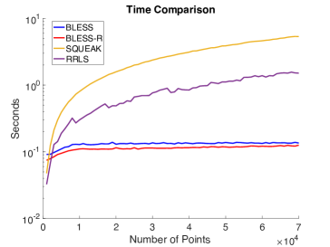
Figure 2: Runtimes with $\lambda=10^{-3}$ and $n$ increasing

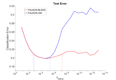
Figure 3: C-err at 5 iterations for varying $\lambda_{falkon}$

4 Experiments

Leverage scores accuracy. We first study the accuracy of the leverage scores generated by BLESS and BLESS-R, comparing SQUEAK [8] and Recursive-RLS (RRLS) [9]. We begin by uniformly sampling a subsets of $n=7\times 10^{4}$ points from the SUSY dataset [19], and computing the exact leverage scores $\ell(i,\lambda)$ using a Gaussian Kernel with $\sigma=4$ and $\lambda=10^{-5}$, which is at the limit of our computational feasibility. We then run each algorithm to compute the approximate leverage scores $\widetilde{\ell}_{J_{H}}(i,\lambda)$, and we measure the accuracy of each method using the ratio $\widetilde{\ell}_{J_{H}}(i,\lambda)/\ell(i,\lambda)$ (R-ACC). The final results are presented in Figure 1. On the left side for each algorithm we report runtime, mean R-ACC, and the $5^{th}$ and $95^{th}$ quantile, each averaged over the 10 repetitions. On the right side a box-plot of the R-ACC. As shown in Figure 1 BLESS and BLESS-R achieve the same optimal accuracy of SQUEAK with just a fraction of time. Note that despite our best efforts, we could not obtain high-accuracy results for RRLS (maybe a wrong constant in the original implementation). However note that RRLS is computationally demanding compared to BLESS, being orders of magnitude slower, as expected from the theory. Finally, although uniform sampling is the fastest approach, it suffers from much larger variance and can over or under-estimate leverage scores by an order of magnitude more than the other methods, making it more fragile for downstream applications.
In Fig. 2 we plot the runtime cost of the compared algorithms as the number of points grows from $n=1000$ to $70000$, this time for $\lambda=10^{-3}$. We see that while previous algorithms’ runtime grows near-linearly with $n$, BLESS and BLESS-R run in a constant $1/\lambda$ runtime, as predicted by the theory.

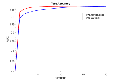
Figure 4: AUC per iteration of the SUSY dataset

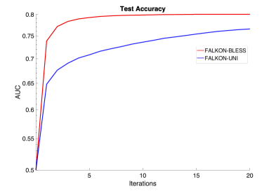
Figure 5: AUC per iteration of the HIGGS dataset

BLESS for supervised learning. We study the performance of FALKON-BLESS and compare it with the original FALKON [14] where an equal number of Nyström centres are sampled uniformly at random (FALKON-UNI). We take from [14] the two biggest datasets and their best hyper-parameters for the FALKON algorithm.
We noticed that it is possible to achieve the same accuracy of FALKON-UNI, by using $\lambda_{bless}$ for BLESS and $\lambda_{falkon}$ for FALKON with $\lambda_{bless}\gg\lambda_{falkon}$, in order to lower the ${d_{\text{eff}}}$ and keep the number of Nyström centres low. For the SUSY dataset we use a Gaussian Kernel with $\sigma=4,\lambda_{falkon}=10^{-6},\lambda_{bless}=10^{-4}$ obtaining $M_{H}\simeq 10^{4}$ Nyström centres. For the HIGGS dataset we use a Gaussian Kernel with $\sigma=22,\lambda_{falkon}=10^{-8},\lambda_{bless}=10^{-6}$, obtaining $M_{H}\simeq 3\times 10^{4}$ Nyström centres. We then sample a comparable number of centers uniformly for FALKON-UNI. Looking at the plot of their AUC at each iteration (Fig.4,5) we observe that FALKON-BLESS converges much faster than FALKON-UNI. For the SUSY dataset (Figure 4) 5 iterations of FALKON-BLESS (160 seconds) achieve the same accuracy of 20 iterations of FALKON-UNI (610 seconds). Since running BLESS takes just $12$ secs. this corresponds to a $\sim 4\times$ speedup. For the HIGGS dataset 10 iter. of FALKON-BLESS (with BLESS requiring $1.5$ minutes, for a total of $1.4$ hours) achieve better accuracy of 20 iter. of FALKON-UNI ($2.7$ hours). Additionally we observed that FALKON-BLESS is more stable than FALKON-UNI w.r.t. $\lambda_{falkon},\sigma$. In Figure 3 the classification error after 5 iterations of FALKON-BLESS and FALKON-UNI over the SUSY dataset ($\lambda_{bless}=10^{-4}$). We notice that FALKON-BLESS has a wider optimal region ($95\%$ of the best error) for the regulariazion parameter ($\small[1.3\times 10^{-3},4.8\times 10^{-8}]$) w.r.t. FALKON-UNI ($\small[1.3\times 10^{-3},3.8\times 10^{-6}]$).

5 Conclusions

In this paper we presented two algorithms BLESS and BLESS-R to efficiently compute a small set of columns from a large symmetric positive semidefinite matrix $K$, useful for approximating the matrix or to compute leverage scores with a given precision. Moreover we applied the proposed algorithms in the context of statistical learning with least squares, combining BLESS with FALKON [14]. We analyzed the computational and statistical properties of the resulting algorithm, showing that it achieves optimal statistical guarantees with a cost that is $O(n{d_{\text{eff}}}^{*}(\lambda))$ in time, being currently the fastest. We can extend the proposed work in several ways: (a) combine BLESS with fast stochastic [20] or online [21] gradient algorithms and other approximation schemes (i.e. random features [22, 23, 24]), to further reduce the computational complexity for optimal rates, (b) consider the impact of BLESS in the context of multi-tasking [25, 26] or structured prediction [27, 28].

Acknowledgments.
This material is based upon work supported by the Center for Brains, Minds and Machines (CBMM), funded by NSF STC award CCF-1231216, and the Italian Institute of Technology. We gratefully acknowledge the support of NVIDIA Corporation for the donation of the Titan Xp GPUs and the Tesla k40 GPU used for this research. L. R. acknowledges the support of the AFOSR projects FA9550-17-1-0390 and BAA-AFRL-AFOSR-2016-0007 (European Office of Aerospace Research and Development), and the EU H2020-MSCA-RISE project NoMADS - DLV-777826. A. R. acknowledges the support of the European Research Council (grant SEQUOIA 724063).

Appendix A Theoretical Analysis for Algorithms 1 and 2

In this section, Thm. 4 and Thm. 5 provide guarantees for the two methods, from which Thm. 1 is derived.

In particular in Section A.4 some important properties about (out-of-sample-)leverage scores, that will be used in the proofs, are derived.

A.1 Notation

Let ${X}$ be a Polish space and $K:{X}\times{X}\to\mathbb{R}$ a positive semidefinite function on ${X}$, we denote $\mathcal{H}$ the Hilbert space obtained by the completion of

$$\mathcal{H}=\overline{\textrm{span}\{K(x,\cdot)\ |\ x\in{X}\}}$$

according to the norm induced by the inner product $\left\langle{K(x,\cdot)},{K(x^{\prime},\cdot)}\right\rangle_{\mathcal{H}}=K(x,x^{\prime})$. Spaces $\mathcal{H}$ constructed in this way are known as reproducing kernel Hilbert spaces and there is a one-to-one relation between a kernel $K$ and its associated RKHS. For more details on RKHS we refer the reader to [29, 30]. Given a kernel $K$, in the following we will denote with $K_{x}=K(x,\cdot)\in\mathcal{H}$ for all $x\in{X}$. We say that a kernel is bounded if $\|K_{x}\|_{\mathcal{H}}\leq\kappa$ with $\kappa>0$. In the following we will always assume $K$ to be continuous and bounded by $\kappa>0$. The continuity of $K$ with the fact that ${X}$ is Polish implies $\mathcal{H}$ to be separable [30].

In the rest of the appdendizes we denote with $A_{\lambda}$, the operator $A+\lambda I$, for any symmetric linear operator $A$, $\lambda\in\mathbb{R}$ and $I$ the identity operator.

A.2 Definitions

For $n\in\mathbb{N}$, $(x_{i})_{i=1}^{n}$, and $J\subseteq\{1,\dots,n\}$, $A\in\mathbb{R}^{|J|\times|J|}$ diagonal matrix with positive diagonal, denote $\widetilde{\ell}_{J}$ in eq. 3 by showing the dependence from both $J$ and $A$ as

$$\widetilde{\ell}_{J,A}(i,\lambda)=(\lambda n)^{-1}(\widehat{K}_{ii}-\widehat{K}_{J,i}^{\top}(\widehat{K}_{J,J}+\lambda nA)^{-1}\widehat{K}_{J,i}).$$ (19)

Moreover define $\widehat{C}_{J,A}$ as follows

$$\widehat{C}_{J,A}=\frac{1}{|J|}\sum_{i=1}^{|J|}A_{ii}^{-1}K_{x_{j_{i}}}\otimes K_{x_{j_{i}}}.$$

We define the out-of-sample leverage scores, that are an extension of $\widetilde{\ell}_{J,A}$ to any point $x$ in the space ${X}$.

Definition 1 (out-of-sample leverage scores).

Let $J=\{j_{1},\dots,j_{M}\}\subseteq\{1,\dots,n\}$, with $M\in\mathbb{N}$ and $A\in\mathbb{R}^{M\times M}$ be a positive diagonal matrix. Then for any $x\in X$ and $\lambda>0$ we define

$$\widehat{\ell}_{J,A}(x,\lambda)=\frac{1}{n}\|(\widehat{C}_{J,A}+\lambda I)^{-1/2}K_{x}\|^{2}_{\mathcal{H}}.$$

Moreover define $\widehat{\ell}_{\emptyset,[]}(x,\lambda)=(\lambda n)^{-1}K(x,x)$.

In particular we denote by

$$\widehat{\ell}(x,\lambda)=\widehat{\ell}_{[n],I}(x,\lambda),$$

the out of sample version of the leverage scores $\ell(i,\lambda)$. Indeed note that $\widehat{\ell}(x_{i},\lambda)=\ell(i,\lambda)$ for $i\in[n]$ and $\lambda>0$ as proven by the next proposition that shows, more generally, the relation between $\widehat{\ell}_{J,A}$ and $\widetilde{\ell}_{J,A}$.

Proposition 1.

Let $n\in\mathbb{N}$, $(x_{i})_{i=1}^{n}\subseteq X$. For any $\lambda>0,J\subseteq\{1,\dots,n\},A\in\mathbb{R}^{|J|\times|J|}$ with $A$ positive diagonal, we that that for any $x\in X$, $\widehat{\ell}_{J,A}(x,\lambda)$ in Def. 1 and $\widetilde{\ell}_{J,A}(x,\lambda)$ in Def. 3, satisfy

$$\widehat{\ell}_{J,\frac{n}{|J|}A}(x_{i},\lambda)=\widetilde{\ell}_{J,A}(i,\lambda),$$

when $|J|>0$, and $\widehat{\ell}_{\emptyset,[]}(x_{i},\lambda)=\widetilde{\ell}_{\emptyset,[]}(i,\lambda)$, when $|J|=0$, for any $i\in[n],\lambda>0$.

Proof.

Let $J=\{j_{1},\dots,j_{|J|}\}$. We will first show that $\widehat{\ell}_{J,A}(x,\lambda)$ is characterized by,

$$\widehat{\ell}_{J,A}(x,\lambda)=\frac{1}{\lambda n}K(x,x)-\frac{1}{\lambda n}v_{J}(x)^{\top}(K_{J}+\lambda|J|A)^{-1}v_{J}(x),$$

with $K_{J}\in\mathbb{R}^{M\times M}$ with $(K_{J})_{lm}=K(x_{j_{l}},x_{j_{m}})$ and $v_{J}(x)=(K(x,x_{j_{1}}),\dots,K(x,x_{j_{M}}))$. Denote with $Z_{J}:\mathcal{H}\to\mathbb{R}^{|J|}$, the linear operator defined by $Z_{J}=(K_{x_{j_{1}}},\dots,K_{x_{j_{|J|}}})^{\top}$, that is $(Z_{J}f)_{k}=\big{<}K_{x_{j_{k}}},f\big{>}_{\mathcal{H}}$, for $f\in\mathcal{H}$ and $k\in\{1,\dots|J|\}$. Then, by denoting with $B=|J|A$ we have

$$Z_{J}^{*}B^{-1}Z_{J}=\frac{1}{|J|}\sum_{i=1}^{|J|}A_{ii}^{-1}K_{x_{j_{i}}}\otimes K_{x_{j_{i}}}=\widehat{C}_{J,A}.$$

Now note that, since $(Q+\lambda I)^{-1}=\lambda^{-1}(I-Q(Q+\lambda I)^{-1})$ for any positive linear operator and $\lambda>0$, we have

$$\widehat{\ell}_{J,A}(x,\lambda) =\frac{1}{n}\left\langle{K_{x}},{(\widehat{C}_{J,A}+\lambda I)^{-1}K_{x}}\right\rangle_{\mathcal{H}}=\frac{1}{\lambda n}\left\langle{K_{x}},{(I-\widehat{C}_{J,A}(\widehat{C}_{J,A}+\lambda I)^{-1})K_{x}}\right\rangle_{\mathcal{H}}$$

$$=\frac{K(x,x)}{\lambda n}-\frac{1}{\lambda n}\left\langle{K_{x}},{Z_{J}^{*}B^{-1/2}(B^{-1/2}Z_{J}Z_{J}^{*}B^{-1/2}+\lambda I)^{-1}B^{-1/2}Z_{J}K_{x}}\right\rangle_{\mathcal{H}},$$

where in the last step we use the fact that $R^{*}R(R^{*}R+\lambda I)^{-1}=R^{*}(RR^{*}+\lambda I)^{-1}R$, for any bounded linear operator $R$ and $\lambda>0$. In particular we used it with $R=B^{-1/2}Z_{J}$. Now note that $Z_{J}Z_{J}^{*}\in\mathbb{R}^{|J|\times|J|}$ and in particular $Z_{J}Z_{J}^{*}=K_{J}$, moreover $Z_{J}K_{x}=v(x)$, so

$$\widehat{\ell}_{J,A}(x,\lambda) =\frac{K(x,x)}{\lambda n}-\frac{1}{\lambda n}v(x)^{\top}B^{-1/2}(B^{-1/2}K_{J}B^{-1/2}+\lambda I)^{-1}B^{-1/2}v(x)$$

$$=\frac{K(x,x)}{\lambda n}-\frac{1}{\lambda n}v(x)^{\top}(K_{J}+\lambda B)^{-1}v(x)$$

$$=\frac{K(x,x)}{\lambda n}-\frac{1}{\lambda n}v(x)^{\top}(K_{J}+\lambda|J|A)^{-1}v(x),$$

where in the second step we used the fact that $B^{-1/2}(B^{-1/2}KB^{-1/2}+\lambda I)^{-1}B^{-1/2}=(K+\lambda B)^{-1}$, for any invertible $B$ any positive operator $K$ and $\lambda>0$.

Finally note that

$$\widehat{\ell}_{J,\frac{n}{|J|}A}(x_{i},\lambda)=\frac{K(x,x)}{\lambda n}-\frac{1}{\lambda n}v(x)^{\top}(K_{J}+\lambda nA)^{-1}v(x)=\widetilde{\ell}_{J,A}(i,\lambda).$$

∎

A.3 Preliminary results

Denote with $G_{\lambda}(A,B)$ the quantity

$$G_{\lambda}(A,B)=\|(A+\lambda I)^{-1/2}(A-B)(A+\lambda I)^{-1/2}\|,$$

for $A,B$ positive bounded linear operators and for $\lambda>0$.

Proposition 2.

Let $A,B$ be positive bounded linear operators and $\lambda>0$, then

$$\|I-(A+\lambda I)^{-1/2}(B+\lambda I)(A+\lambda I)^{-1/2}\|=G_{\lambda}(A,B)\leq\frac{G_{\lambda}(B,A)}{1-G_{\lambda}(B,A)},$$

where the last inequality holds if $G_{\lambda}(B,A)<1$.

Proof.

For the sake of compactness denote with $A_{\lambda}$ the operator $A+\lambda I$ and with $B_{\lambda}$ the operator $B+\lambda I$. First of all note that $I=A_{\lambda}^{-1/2}A_{\lambda}A_{\lambda}^{-1/2}$, so

$$I-A_{\lambda}^{-1/2}B_{\lambda}A_{\lambda}^{-1/2} =A_{\lambda}^{-1/2}A_{\lambda}A_{\lambda}^{-1/2}-A_{\lambda}^{-1/2}B_{\lambda}A_{\lambda}^{-1/2}$$

$$=A_{\lambda}^{-1/2}(A_{\lambda}-B_{\lambda})A_{\lambda}^{-1/2}=A_{\lambda}^{-1/2}(A-B)A_{\lambda}^{-1/2}$$

$$=A_{\lambda}^{-1/2}B_{\lambda}^{1/2}~{}~{}B_{\lambda}^{-1/2}(A-B)B_{\lambda}^{-1/2}~{}~{}B_{\lambda}^{1/2}A_{\lambda}^{-1/2},$$

where in the last step we multiplied and divided by $B_{\lambda}^{1/2}$. Then

$$\lVert{I-A_{\lambda}^{-1/2}B_{\lambda}A_{\lambda}^{-1/2}}\rVert\leq\|A_{\lambda}^{-1/2}B_{\lambda}^{1/2}\|^{2}\|B_{\lambda}^{-1/2}(A-B)B_{\lambda}^{-1/2}\|,$$

moreover, by Prop. 7 of [15] (see also Prop. 8 of [23]), if $G_{\lambda}(B,A)<1$, we have

$$\|A_{\lambda}^{-1/2}B_{\lambda}^{1/2}\|^{2}\leq(1-G_{\lambda}(B,A))^{-1}.$$

∎

Proposition 3.

Let $A,B,C$ be bounded positive linear operators on a Hilbert space. Let $\lambda>0$. Then, the following holds

$$G_{\lambda}(A,C)\leq G_{\lambda}(A,B)+(1+G_{\lambda}(A,B))G_{\lambda}(B,C).$$

Proof.

In the following we denote with $A_{\lambda}$ the operator $A+\lambda I$ and the same for $B,C$. Then

$$\|A_{\lambda}^{-1/2}(A-C)A_{\lambda}^{-1/2}\|\leq\|A_{\lambda}^{-1/2}(A-B)A_{\lambda}^{-1/2}\|+\|A_{\lambda}^{-1/2}(B-C)A_{\lambda}^{-1/2}\|.$$

Now note that, by dividing and multiplying for $B_{\lambda}^{1/2}$, we have

$$\|A_{\lambda}^{-1/2}(B-C)A_{\lambda}^{-1/2}\| =\|A_{\lambda}^{-1/2}B_{\lambda}^{1/2}~{}B_{\lambda}^{-1/2}(B-C)B_{\lambda}^{-1/2}B_{\lambda}^{1/2}A_{\lambda}^{-1/2}\|$$

$$\leq\|A_{\lambda}^{-1/2}B_{\lambda}^{1/2}\|^{2}\|B_{\lambda}^{-1/2}(B-C)B_{\lambda}^{-1/2}\|=\|A_{\lambda}^{-1/2}B_{\lambda}^{1/2}\|^{2}G_{\lambda}(B,C).$$

Finally note that, since $\lVert{Z}\rVert^{2}=\lVert{Z^{*}Z}\rVert$ for any bounded linear operator $Z$, we have

$$\|A_{\lambda}^{-1/2}B_{\lambda}^{1/2}\|^{2} =\|A_{\lambda}^{-1/2}B_{\lambda}A_{\lambda}^{-1/2}\|=\|I+(I-A_{\lambda}^{-1/2}B_{\lambda}A_{\lambda}^{-1/2})\|\leq 1+\|I-A_{\lambda}^{-1/2}B_{\lambda}A_{\lambda}^{-1/2}\|.$$

Moreover, by Prop. 2, we have that

$$\|I-A_{\lambda}^{-1/2}B_{\lambda}A_{\lambda}^{-1/2}\|=G_{\lambda}(A,B).$$

∎

Proposition 4.

Let $B$ be a bounded linear operator, then

$$1-\|I-BB^{*}\|\leq\sigma_{\min}(B)^{2}\leq\sigma_{\max}(B)^{2}\leq 1+\|I-BB^{*}\|.$$

Proof.

Now we recall that, denoting by $\preceq$ the Lowner partial order, for a positive bounded operator $A$ such that $aI\preceq A\preceq bI$ for $0\leq a\leq b$, we have $(1-b)I\preceq I-A\preceq(1-a)I\preceq(1+b)I$ and so, since $BB^{*}=I-(I-BB^{*})$, we have

$$(1-\|I-BB^{*}\|)I\preceq\sigma_{\min}(B)^{2}I\preceq BB^{*}\preceq\sigma_{\max}(B)^{2}I\preceq 1+(1+\|I-BB^{*}\|)I,$$

from we have the desired result. ∎

Let $\lVert{\cdot}\rVert_{HS}$ denote the Hilbert-Schmidt norm.

We recall and adapt to our needs a result from Prop. 8 of [15].

Proposition 5.

Let $\lambda>0$ and $v_{1},\dots,v_{n}$ with $n\geq 1$, be identically distributed random vectors on separable Hilbert space $\mathcal{H}$, such that there exists $\kappa^{2}>0$ for which $\|v\|_{\mathcal{H}}\leq\kappa^{2}$ almost surely. Denote by $Q$ the Hermitian operator $Q=\frac{1}{n}\sum_{i=1}^{n}{\mathbb{E}}[v_{i}\otimes v_{i}]$. Let $Q_{n}=\frac{1}{n}\sum_{i=1}^{n}v_{i}\otimes v_{i}$. Then for any $\delta\in(0,1]$, the following holds

$$\lVert{(Q+\lambda I)^{-1/2}(Q-Q_{n})(Q+\lambda I)^{-1/2}}\rVert{}\leq\frac{4\kappa^{2}\beta}{3\lambda n}+\sqrt{\frac{2\kappa^{2}\beta}{\lambda n}}$$

with probability $1-\delta$ and $\beta=\log\frac{4\operatorname{Tr}(Q(Q+\lambda I)^{-1})}{\lVert{Q(Q+\lambda I)^{-1}}\rVert{}\delta}\leq\frac{8\kappa^{2}(1+\operatorname{Tr}(Q_{\lambda}^{-1}Q))}{\|Q\|\delta}$.

Proof.

Let $Q_{\lambda}=Q+\lambda I$. Here we apply non-commutative Bernstein inequality like [3] (with the extension to separable Hilbert spaces as in[15], Prop. 12) on the random variables $Z_{i}=M-Q_{\lambda}^{-1/2}v_{i}\otimes Q_{\lambda}^{-1/2}v_{i}$ with $M_{i}=Q_{\lambda}^{-1/2}({\mathbb{E}}[v_{i}\otimes v_{i}])Q_{\lambda}^{-1/2}$ for $1\leq i\leq n$. Note that the expectation of $Z_{i}$ is $0$. The random vectors are bounded by

$$\|Q_{\lambda}^{-1/2}v_{i}\otimes Q_{\lambda}^{-1/2}v_{i}-M_{i}\| =\|\mathbb{E}_{v^{\prime}_{i}}[Q_{\lambda}^{-1/2}v^{\prime}_{i}\otimes Q_{\lambda}^{-1/2}v^{\prime}_{i}-Q_{\lambda}^{-1/2}v_{i}\otimes Q_{\lambda}^{-1/2}v_{i}]\|_{\mathcal{H}}$$

$$\leq 2\|\kappa^{2}\|\|(Q+\lambda)^{-1/2}\|^{2}\leq\frac{2\kappa^{2}}{\lambda},$$

and the second orded moment is

$$\mathbb{E}(Z_{i})^{2} =\mathbb{E}\;\;\left\langle{v_{i}},{Q_{\lambda}^{-1}v_{i}}\right\rangle\;Q_{\lambda}^{-1/2}v_{i}\otimes Q_{\lambda}^{-1/2}v_{i}\;\;\;-\;\;\;Q_{\lambda}^{-2}Q^{2}$$

$$\leq\frac{\kappa^{2}}{\lambda}{\mathbb{E}}[Q_{\lambda}^{-1/2}v_{1}\otimes Q_{\lambda}^{-1/2}v_{1}]=\frac{\kappa^{2}}{\lambda}Q(Q+\lambda I)^{-1}=:S.$$

Now we can apply the Bernstein inequality with intrinsic dimension in [3] (or Prop. 12 in [15]). Now some considerations on $\beta$. It is $\beta=\log\frac{4\operatorname{Tr}S}{\lVert{S}\rVert{}\delta}=\frac{4\operatorname{Tr}Q_{\lambda}^{-1}Q}{\lVert{Q_{\lambda}^{-1}Q}\rVert{}\delta}$, now we need a lower bound for $\lVert{Q_{\lambda}^{-1}Q}\rVert{}=\frac{\sigma_{1}}{\sigma_{1}+\lambda}$ where $\sigma_{1}=\lVert{Q}\rVert$ is the biggest eigenvalue of $Q$, now, when $0<\lambda\leq\sigma_{1}$ we have $\beta\leq\frac{8\operatorname{Tr}Q}{\lambda\delta}$.

When $\lambda\geq\sigma_{1}$, note that $\operatorname{Tr}(Q(Q+\lambda I)^{-1})\leq\lambda^{-1}\operatorname{Tr}(Q)\leq\kappa^{2}/\lambda$, then

$$\frac{\operatorname{Tr}(Q(Q+\lambda I)^{-1})}{\lVert{Q_{\lambda}^{-1}Q}\rVert}\leq\frac{\kappa^{2}}{\lambda\frac{\sigma_{1}}{\sigma_{1}+\lambda}}=\frac{\kappa^{2}}{\lambda}+\frac{\kappa^{2}}{\sigma_{1}}\leq\frac{2\kappa^{2}}{\sigma_{1}}.$$

So finally $\beta\leq\frac{8(\kappa^{2}/\|Q\|+\operatorname{Tr}(Q_{\lambda}^{-1}Q))}{\delta}$ ∎

A.4 Analytic decomposition

Lemma 2.

Let $\lambda>0$, $J,J^{\prime}\subseteq\{1,\dots,n\}$, with $|J|,|J^{\prime}|\geq 1$ and $A\in\mathbb{R}^{|J|\times|J|}$, $A^{\prime}\in\mathbb{R}^{|J^{\prime}|\times|J^{\prime}|}$ positive diagonal matrices, then

$$\frac{1-2\nu}{1-\nu}\widehat{\ell}_{J^{\prime},A^{\prime}}(x,\lambda)\leq\widehat{\ell}_{J,A}(x,\lambda)\leq\frac{1}{1-\nu}\widehat{\ell}_{J^{\prime},A^{\prime}}(x,\lambda),\quad\forall x\in{X},$$

with $\nu=G_{\lambda}(\widehat{C}_{J^{\prime},A^{\prime}},\widehat{C}_{J,A})$.

Proof.

By denoting with $B$ the operator

$$B=(\widehat{C}_{J,A}+\lambda I)^{-1/2}(\widehat{C}_{J^{\prime},A^{\prime}}+\lambda I)^{1/2},$$

and according to the characterization of $\widehat{\ell}_{J,A}(x,\lambda)$ via Prop. 1, we have

$$\widehat{\ell}_{J,A}(x,\lambda) =n^{-1}\lVert{(\widehat{C}_{J,A}+\lambda I)^{-1/2}K_{x}}\rVert^{2}_{\mathcal{H}}=n^{-1}\lVert{B~{}(\widehat{C}_{J^{\prime},A^{\prime}}+\lambda I)^{-1/2}K_{x}}\rVert^{2}_{\mathcal{H}}.$$

So, by recalling the fact that, by definition of Lowner partial order $\preceq$, we have $a\|v\|^{2}\leq\|Av\|^{2}\leq b\|v\|^{2}$, for any vector $v$ and bounded linear operator such that $aI\preceq A^{*}A\preceq bI$ with $0\leq a\leq b$, and the fact that $\sigma(A^{*}A)=\sigma(AA^{*})=\sigma(A)^{2}$, we have

$$\sigma_{\min}(B)^{2}\lVert{(\widehat{C}_{J^{\prime},A^{\prime}}+\lambda I)^{-1/2}K_{x}}\rVert^{2}_{\mathcal{H}}\leq\lVert{B(\widehat{C}_{J^{\prime},A^{\prime}}+\lambda I)^{-1/2}K_{x}}\rVert^{2}_{\mathcal{H}}\leq\sigma_{\max}(B)^{2}\lVert{(\widehat{C}_{J^{\prime},A^{\prime}}+\lambda I)^{-1/2}K_{x}}\rVert^{2}_{\mathcal{H}}.$$

That, by Prop. 1, is equivalent to

$$\sigma_{\min}(B)^{2}\widehat{\ell}_{J^{\prime},A^{\prime}}(x,\lambda)\leq\widehat{\ell}_{J,A}(x,\lambda)\leq\sigma_{\max}(B)^{2}\widehat{\ell}_{J^{\prime},A^{\prime}}(x,\lambda).$$

By Prop. 4 we have $1-\|I-BB^{*}\|\leq\sigma_{\min}(B)^{2}\leq\sigma_{\max}(B)^{2}\leq 1+\|I-BB^{*}\|$. Finally, by Prop. 2, we have

$$\|I-BB^{*}\|\leq\frac{\nu}{1-\nu}.$$

∎

Lemma 3.

Let $0<\lambda\leq\lambda^{\prime}$, and $J\subseteq\{1,\dots,n\}$ and $A\in\mathbb{R}^{|J|\times|J|}$, then

$$\widehat{\ell}_{J,A}(x,\lambda^{\prime})\leq\widehat{\ell}_{J,A}(x,\lambda)\leq\frac{\lambda^{\prime}}{\lambda}\widehat{\ell}_{J,A}(x,\lambda^{\prime}),\quad\forall x\in{X}.$$

Proof.

If $|J|=0$ we have that $\widehat{\ell}_{\emptyset,[]}(x,\lambda)=\frac{K(x,x)}{\lambda n}$ and the desired result is easily verified. If $|J|\geq 1$, let $B=(C_{J,A}+\lambda I)^{-1/2}(C_{J,A}+\lambda^{\prime}I)^{1/2}$. By recalling the fact that, by definition of Lowner partial order $\preceq$, we have $a\|v\|^{2}\leq\|Av\|^{2}\leq b\|v\|^{2}$, for any vector $v$ and bounded linear operator such that $aI\preceq A^{*}A\preceq bI$ with $0\leq a\leq b$, and the fact that $\sigma(A^{*}A)=\sigma(AA^{*})=\sigma(A)^{2}$, we have

$$\sigma_{\min}(B)^{2}\lVert{(\widehat{C}_{J,A}+\lambda^{\prime}I)^{-1/2}K_{x}}\rVert^{2}_{\mathcal{H}}\leq\lVert{B(\widehat{C}_{J,A}+\lambda^{\prime}I)^{-1/2}K_{x}}\rVert^{2}_{\mathcal{H}}\leq\sigma_{\max}(B)^{2}\lVert{(\widehat{C}_{J,A}+\lambda^{\prime}I)^{-1/2}K_{x}}\rVert^{2}_{\mathcal{H}}.$$

That, by Prop. 1, is equivalent to

$$\sigma_{\min}(B)^{2}\widehat{\ell}_{J,A}(x,\lambda^{\prime})\leq\widehat{\ell}_{J,A}(x,\lambda)\leq\sigma_{\max}(B)^{2}\widehat{\ell}_{J,A}(x,\lambda^{\prime}).$$

Now note that

$$\sigma_{\min}(B)^{2}\geq\inf_{\sigma\geq 0}\frac{\sigma+\lambda^{\prime}}{\sigma+\lambda}=1,\quad\sigma_{\max}(B)^{2}\geq\sup_{\sigma\geq 0}\frac{\sigma+\lambda^{\prime}}{\sigma+\lambda}=\frac{\lambda^{\prime}}{\lambda}.$$

∎

Theorem 3.

Let $\lambda>0$, $J\subseteq\{1,\dots,n\}$, with $|J|\geq 1$ and $A\in\mathbb{R}^{|J|\times|J|}$ positive diagonal. Then the following hold for any $x\in X$,

$$\frac{1-2\nu_{J,A}}{1-\nu_{J,A}}\widehat{\ell}(x,\lambda)\leq\widehat{\ell}_{J,A}(x,\lambda)\leq\frac{1}{1-\nu_{J,A}}\widehat{\ell}(x,\lambda),$$

where $\nu_{J,A}=G_{\lambda}(\widehat{C},\widehat{C}_{J,A})$. Morever note that for any $|U|\subseteq\{1,\dots,n\}$, we have

$$\nu_{J,A}\leq\eta_{U}+(1+\eta_{U})\beta_{J,A,U},$$

with $\beta_{J,A,U}=G_{\lambda}(\widehat{C}_{U,I},\widehat{C}_{J,A})$ and $\eta_{U}=G_{\lambda}(\widehat{C},\widehat{C}_{U,I})$.

Proof.

By applying Lemma 2, with their $J^{\prime}=\{1,\dots,n\},A^{\prime}=I$, and recalling that $\widehat{\ell}(x,\lambda)=\widehat{\ell}_{\{1,\dots,n\},I}$, we have for all $x\in{X}$

$$\frac{1-2\nu_{J,A}}{1-\nu_{J,A}}\widehat{\ell}(x,\lambda)\leq\widehat{\ell}_{J,A}(x,\lambda)\leq\frac{1}{1-\nu_{J,A}}\widehat{\ell}(x,\lambda).$$

To conclude the proof we bound $\nu_{J,A}$ in terms of $\beta_{J,A,U}$ and $\eta_{U}$, via Prop. 3. ∎

A.5 Proof for Algorithm 1

Lemma 4.

Let $n\in\mathbb{N}$, $(x_{i})_{i=1}^{n}\subseteq{X}$. Let $U\subseteq\{1,\dots n\}$, with $|U|\geq 1$. Let $(p_{k})_{k=1}^{|U|}\subset\mathbb{R}$ be a non-negative sequence summing to $1$. Let $M\in\mathbb{N}$ and $J=\{j_{1},\dots,j_{M}\}$ with $j_{i}$ sampled i.i.d. from $\{1,\dots,|U|\}$ with probability $(p_{k})_{k=1}^{|U|}$ and $A=|U|\textrm{diag}(p_{j_{1}},\dots,p_{j_{M}})$. Let $\tau\in(0,1]$, and $s:=\sup_{k\in\{1,\dots,|U|\}}\frac{1}{|U|p_{k}}\|(\widehat{C}_{U,I}+\lambda I)^{-1/2}K_{x_{u_{k}}}\|_{\mathcal{H}}^{2}$. When

$$M\geq 2s\log\frac{4n}{\tau},$$

then the following holds with probability at least $1-\tau$

$$\|(\widehat{C}_{U,I}+\lambda I)^{-1/2}(\widehat{C}_{J,A}-\widehat{C}_{U,I})(\widehat{C}_{U,I}+\lambda I)^{-1/2}\|\leq\sqrt{\frac{4s\log\frac{4n}{\tau}}{M}}.$$

Proof.

Denote with $\zeta_{i}$ the random variable

$$\zeta_{i}=\frac{1}{|U|p_{k}}(\widehat{C}_{U,I}+\lambda I)^{-1/2}(K_{x_{j_{i}}}\otimes K_{x_{j_{i}}})(\widehat{C}_{U,I}+\lambda I)^{-1/2},$$

for $i\in\{1,\dots,M\}$. In particular note that $\zeta_{1},\dots,\zeta_{M}$ are i.i.d. since $j_{1},\dots,j_{M}$ are. Moreover note the following two facts

$$\|\zeta_{i}\| =\sup_{k\in\{1,\dots,|U|\}}\frac{1}{|U|p_{k}}\|(\widehat{C}_{U,I}+\lambda I)^{-1/2}K_{x_{u_{k}}}\|_{\mathcal{H}}^{2}=s,$$

$${\mathbb{E}}[\zeta_{i}] =\sum_{k=1}^{|U|}p_{k}~{}\frac{1}{|U|p_{k}}(\widehat{C}_{U,I}+\lambda I)^{-1/2}(K_{x_{k}}\otimes K_{x_{k}})(\widehat{C}_{U,I}+\lambda I)^{-1/2}$$

$$=(\widehat{C}_{U,I}+\lambda I)^{-1/2}\widehat{C}_{U,I}(\widehat{C}_{U,I}+\lambda I)^{-1/2}=:W,$$

where for the second identity we used the fact that $d/l_{k}=1/(p_{k}|U|)$. Since by definition of $\widehat{C}_{J,A}$ we have

$$\frac{1}{M}\sum_{i=1}^{M}\zeta_{i} =(\widehat{C}_{U,I}+\lambda I)^{-1/2}\left(\frac{1}{|J|}\sum_{i=1}^{M}\frac{1}{A_{ii}}K_{x_{j_{i}}}\otimes K_{x_{j_{i}}}\right)(\widehat{C}_{U,I}+\lambda I)^{-1/2}$$

$$=(\widehat{C}_{U,I}+\lambda I)^{-1/2}\widehat{C}_{J,A}(\widehat{C}_{U,I}+\lambda I)^{-1/2},$$

then, by applying non-commutative Bernstein inequality (Prop. 5 is a version specific for our problem), we have

$$\|(\widehat{C}_{U,I}+\lambda I)^{-1/2}(\widehat{C}_{J,A}-\widehat{C}_{U,I})(\widehat{C}_{U,I}+\lambda I)^{-1/2}\| =\big{\|}\frac{1}{M}\sum_{i=1}^{M}(\zeta_{i}-{\mathbb{E}}[\zeta_{i}])\big{\|}\leq\frac{2s\eta}{3M}+\sqrt{\frac{2s\|W\|\eta}{M}},$$

with probability at least $1-\tau$, and $\eta:=\log\frac{4\operatorname{Tr}(W)}{\tau\|W\|}$. In particular, by noting that $\|W\|\leq 1$ by definition, when $M\geq 2s\eta$, then

$$\frac{2s\eta}{3M}+\sqrt{\frac{2s\|W\|\eta}{M}}\leq\frac{2s\eta}{3M}+\sqrt{\frac{2s\eta}{M}}\leq\frac{1}{3}\sqrt{\frac{2s\eta}{M}}+\sqrt{\frac{2s\eta}{M}}\leq\sqrt{\frac{4s\eta}{M}}.$$

To conclude note that $\frac{\operatorname{Tr}(W)}{\|W\|}\leq\textrm{rank}(W)\leq|U|\leq n$, so $\eta\leq\log\frac{4n}{\tau}$. ∎

Lemma 5.

Let $n,R\in\mathbb{N}$, $(x_{i})_{i=1}^{n}\subseteq{X}$. Let $U=\{u_{1},\dots,u_{R}\}$ with $u_{i}$ i.i.d. with uniform probability on $\{1,\dots,n\}$. Let $\tau\in(0,1]$ and let $\lambda>0$. When

$$R\geq\frac{2n\kappa^{2}}{\lambda n+\kappa^{2}}\log\frac{4n}{\tau},$$

then the following holds with probability $1-\tau$

$$\|(\widehat{C}+\lambda I)^{-1/2}(\widehat{C}_{U,I}-\widehat{C})(\widehat{C}+\lambda I)^{-1/2}\|\leq\sqrt{\frac{4n\kappa^{2}\log\frac{4n}{\tau}}{(\lambda n+\kappa^{2})R}}.$$

Proof.

Denote by $\zeta_{i}$ the random variable $\zeta_{i}=(\widehat{C}+\lambda I)^{-1/2}(K_{x_{u_{i}}}\otimes K_{x_{u_{i}}})(\widehat{C}+\lambda I)^{-1/2}$, for $i\in\{1,\dots,R\}$. Note that $\zeta_{i}$ are i.i.d. since $u_{i}$ are. Moreover note that

$$\|\zeta_{i}\| =\sup_{i\in\{1,\dots,n\}}\|(\widehat{C}+\lambda I)^{-1/2}K_{x_{i}}\|^{2}\leq\sup_{i\in\{1,\dots,n\}}\|(\frac{1}{n}K_{x_{i}}\otimes K_{x_{i}}+\lambda I)^{-1/2}K_{x_{i}}\|^{2}$$

$$\leq\frac{n\kappa^{2}}{\lambda n+\kappa^{2}}=:v.$$

Moreover note that

$${\mathbb{E}}[\zeta_{i}]=\frac{1}{n}\sum_{i=1}^{n}(\widehat{C}+\lambda I)^{-1/2}(K_{x_{i}}\otimes K_{x_{i}})(\widehat{C}+\lambda I)^{-1/2}=(\widehat{C}+\lambda I)^{-1/2}\widehat{C}(\widehat{C}+\lambda I)^{-1/2}=:W.$$

So we have, by non-commutative Bernstein inequality (Prop. 5 is a version specific for our problem),

$$\|(\widehat{C}+\lambda I)^{-1/2}(\widehat{C}_{U,I}-\widehat{C})(\widehat{C}+\lambda I)^{-1/2}\|=\big{\|}\frac{1}{M}\sum_{i=1}^{M}(\zeta_{i}-{\mathbb{E}}[\zeta_{i}])\big{\|}\leq\frac{2v\eta}{3R}+\sqrt{\frac{2v\|W\|\eta}{R}},$$

with probability at least $1-\tau$, and $\eta:=\log\frac{4\operatorname{Tr}(W)}{\tau\|W\|}$. In particular, by noting that $\|W\|\leq 1$ by definition, when $R\geq\frac{2n\kappa^{2}\eta}{(\lambda n+\kappa^{2})R}$, analogously to the end of the proof of Lemma 4, we have $\frac{2v\eta}{3R}+\sqrt{\frac{2v\|W\|\eta}{R}}\leq\sqrt{\frac{4n\kappa^{2}\eta}{(\lambda n+\kappa^{2})R}}.$ To conclude note that $\frac{\operatorname{Tr}(W)}{\|W\|}\leq\textrm{rank}(W)\leq n$, so $\eta\leq\log\frac{4n}{\tau}$. ∎

Lemma 6.

Let $n,R\in\mathbb{N}$, $(x_{i})_{i=1}^{n}\subseteq{X}$. Let $U=\{u_{1},\dots,u_{R}\}$ with $u_{i}$ i.i.d. with uniform probability on $\{1,\dots,n\}$. Let $\tau\in(0,1]$ and let $\lambda>0$. When

$$R\geq\frac{16n\kappa^{2}}{\lambda n+\kappa^{2}}\log\frac{4n}{\tau},$$

then the following holds with probability $1-\tau$

$$\frac{n}{R}\sum_{i=1}^{R}\widehat{\ell}(x_{u_{i}},\lambda)<\max\left(5,\frac{6}{5}{d_{\text{eff}}}(\lambda)\right).$$

Proof.

First of all denote with $z_{i}$ the random variable $z_{i}=\frac{n}{R}\widehat{\ell}(x_{u_{i}},\lambda)$ and note that $(z_{i})_{i=1}^{R}$ are $i.i.d.$ since $(u_{i})_{i=1}^{R}$ are. Moreover, by the characterization of $\widehat{\ell}(x,\lambda)$ via Prop. 1, we have

$$|z_{i}|\leq\sup_{k\in\{1,\dots,n\}}\|(\widehat{C}+\lambda I)^{-1/2}K_{x_{k}}\|^{2}\leq\|(K_{x_{k}}\otimes K_{x_{k}}/n+\lambda I)^{1/2}K_{x_{k}}\|^{2}\leq\frac{\kappa^{2}}{R(\kappa^{2}/n+\lambda)}=:v,$$

moreover we have

$${\mathbb{E}}[z_{i}] ={\mathbb{E}}[\operatorname{Tr}((\widehat{C}+\lambda I)^{-1}(K_{x_{u_{i}}}\otimes K_{x_{u_{i}}}))]=\operatorname{Tr}((\widehat{C}+\lambda I)^{-1}{\mathbb{E}}[K_{x_{u_{i}}}\otimes K_{x_{u_{i}}}])$$

$$=\operatorname{Tr}\left((\widehat{C}+\lambda I)^{-1}\sum_{k=1}^{n}\frac{1}{n}K_{x_{k}}\otimes K_{x_{k}}\right)=\operatorname{Tr}\left((\widehat{C}+\lambda I)^{-1}\widehat{C}\right)={d_{\text{eff}}}(\lambda).$$

So by applying Bernstein inequality, the following holds with probability at least $1-\tau$

$$\left|\frac{n}{R}\sum_{i=1}^{R}\widehat{\ell}(x_{u_{i}},\lambda)-{d_{\text{eff}}}(\lambda)\right|=\left|\frac{1}{R}\sum_{i=1}^{R}(z_{i}-{\mathbb{E}}[z_{i}])\right|\leq\frac{2v\log\frac{2}{\tau}}{3R}+\sqrt{\frac{2v{d_{\text{eff}}}(\lambda)\log\frac{2}{\tau}}{3R}}.$$

So we have

$$\frac{n}{R}\sum_{i=1}^{R}\widehat{\ell}(x_{u_{i}},\lambda)\leq{d_{\text{eff}}}(\lambda)+\left|\frac{n}{R}\sum_{i=1}^{R}\widehat{\ell}(x_{u_{i}},\lambda)-{d_{\text{eff}}}(\lambda)\right|\leq{d_{\text{eff}}}(\lambda)+\frac{2v\log\frac{2}{\tau}}{3R}+\sqrt{\frac{2v{d_{\text{eff}}}(\lambda)\log\frac{2}{\tau}}{R}}.$$

Now, if ${d_{\text{eff}}}(\lambda)\leq 4$, since $R\geq 16v\log\frac{2}{\tau}$, we have that

$${d_{\text{eff}}}(\lambda)+\frac{2v\log\frac{2}{\tau}}{3R}+\sqrt{\frac{2v{d_{\text{eff}}}(\lambda)\log\frac{2}{\tau}}{R}}\leq 4+\frac{1}{24}+\sqrt{\frac{1}{2}}<5.$$

If ${d_{\text{eff}}}(\lambda)>4$, since $R\geq 16v\log\frac{2}{\tau}$, we have

$${d_{\text{eff}}}(\lambda)+\frac{2v\log\frac{2}{\tau}}{3R}+\sqrt{\frac{2v{d_{\text{eff}}}(\lambda)\log\frac{2}{\tau}}{3R}} \leq\left(1+\frac{1}{24{d_{\text{eff}}}(\lambda)}+\sqrt{\frac{1}{8{d_{\text{eff}}}(\lambda)}}\right){d_{\text{eff}}}(\lambda)<\frac{6}{5}{d_{\text{eff}}}(\lambda).$$

∎

Theorem 4.

Let $n\in\mathbb{N}$, $(x_{i})_{i=1}^{n}\subseteq X$. Let $\delta\in(0,1]$,  $t,q>1$, $\lambda>0$ and $H,d_{h},\lambda_{h},J_{h},A_{h},U_{h}$ as in Alg. 1. Let $\bar{A}_{h}=\frac{n}{|J|}A_{h}$ and $\nu_{h}=G_{\lambda_{h}}(\widehat{C},\widehat{C}_{J_{h},\bar{A}_{h}})$,  $\beta_{h}=G_{\lambda_{h}}(\widehat{C}_{U_{h},I},\widehat{C}_{J_{h},\bar{A}_{h}})$,  $\eta_{h}=G_{\lambda_{h}}(\widehat{C},\widehat{C}_{U_{h},I})$. When

$$\lambda_{0}=\frac{\kappa^{2}}{\min(t,1)},\quad q_{1}\geq\frac{5\kappa^{2}q_{2}}{q(1+t)},\quad q_{2}\geq 12q{(2t+1)^{2}\over t^{2}}(1+t)\log\frac{12Hn}{\delta},$$

then the following holds with probability $1-\delta$: for any $h\in\{0,\dots,H\}$

$$\begin{split}a)&\qquad\frac{1}{T}\widehat{\ell}(x,\lambda_{h})~{}\leq~{}\widehat{\ell}_{J_{h},\bar{A}_{h}}(x)~{}\leq~{}\min(T,2)\widehat{\ell}(x,\lambda_{h}),~{}~{}~{}\forall x\in X,\\ b)&\qquad d_{h}~{}~{}\leq~{}~{}3q~{}{d_{\text{eff}}}(\lambda_{h})~{}\vee~{}10q,~{}~{}\textrm{and}~{}~{}|J_{h}|\leq q_{2}(3q{d_{\text{eff}}}(\lambda_{h})\vee 10q).\\ c)&\qquad\beta_{h}\leq\frac{7}{11c_{T}},~{}~{}\eta_{h}\leq\frac{3}{11c_{T}},~{}~{}\nu_{h}\leq\frac{1}{c_{T}}.\end{split}$$ (20)

where $T=1+t$ and $c_{T}=2+1/(T-1)$.

Proof.

Let $H$, $c_{T}$, $q$ and $\lambda_{h},U_{h},J_{h},A_{h},d_{h},P_{h}=(p_{h,k})_{k=1}^{R_{h}}$, for $h\in\{0,\dots,H\}$ as defined in Alg. 1 and define $\tau=\delta/(3H)$. Now we are going to define some events and we prove a recurrence relation that they satisfy. Finally we unroll the recurrence relation and bound the resulting events in probability.

Definitions of the events

Now we are going to define some events that will be useful to prove the theorem. Denote with $E_{h}$ the event such that the conditions in Eq. (20)-(a) hold for $J_{h},A_{h},U_{h}$. Denote with $F_{h}$ the event such that

$$\frac{n}{R_{h}}\sum_{u\in U_{h}}\widehat{\ell}(x_{u},\lambda_{h-1})\leq\frac{6}{5}{d_{\text{eff}}}(\lambda).$$

Denote with $B_{1,h}$ the event such that $\beta_{h}$, satisfies

$$\beta_{h}\leq\sqrt{\frac{4s_{h}\log\frac{4n}{\tau}}{M_{h}}},\quad\textrm{with}\quad s_{h}:=\sup_{k\in\{1,\dots,R_{h}\}}\frac{1}{R_{h}p_{h,k}}\|(\widehat{C}_{U_{h},I}+\lambda_{h}I)^{-1/2}K_{x_{u_{k}}}\|^{2}.$$ (21)

Denote with $B_{2,h}$ the event such that $\eta_{h}$, satisfies

$$\eta_{h}\leq\sqrt{\frac{4\kappa^{2}n\log\frac{\kappa^{2}}{\lambda_{h}\tau}}{(\lambda_{h}n+\kappa^{2})R_{h}}}.$$

First bound for $s_{h}$.

Note that, by definition of $p_{h,k}$, that is, by Prop. 1

$$p_{h,k}=n\widetilde{\ell}_{J_{h-1},A_{h-1}}(x_{u_{k}},\lambda_{h})/(d_{h}R_{h})=n\widehat{\ell}_{J_{h-1},\bar{A}_{h-1}}(x_{u_{k}},\lambda_{h})/(d_{h}R_{h}),$$

so

$$s_{h}=\sup_{k\in\{1,\dots,R_{h}\}}\frac{d_{h}\|(\widehat{C}_{U_{h},I}+\lambda_{h}I)^{-1/2}K_{x_{u_{k}}}\|^{2}}{n\widehat{\ell}_{J_{h-1},\bar{A}_{h-1}}(x_{u_{k}},\lambda_{h})}=\sup_{u\in U_{h}}\frac{d_{h}\widehat{\ell}_{U_{h},I}(x_{u},\lambda_{h})}{\widehat{\ell}_{J_{h-1},\bar{A}_{h-1}}(x_{u},\lambda_{h})},$$

where the last step consists in apply the definition of $\widehat{\ell}_{U_{h},I}$. By applying Lemma 2 and 3 to $\widehat{\ell}_{U_{h},I}(x,\lambda_{h})$, we have

$$\widehat{\ell}_{U_{h},I}(x,\lambda_{h}) \leq\frac{1}{1-\eta_{h}}\widehat{\ell}(x,\lambda_{h})\leq\frac{\lambda_{h-1}}{\lambda_{h}(1-\eta_{h})}\widehat{\ell}(x,\lambda_{h-1})$$

and analogously by applying Lemma 3 to $\widehat{\ell}_{J_{h-1},\bar{A}_{h-1}}(x,\lambda_{h})$, we have $\widehat{\ell}_{J_{h-1},\bar{A}_{h-1}}(x,\lambda_{h})\geq\widehat{\ell}_{J_{h-1},\bar{A}_{h-1}}(x,\lambda_{h-1})$. So, by extending the $\sup$ of $s_{h}$ to the whole ${X}$, we have

$$s_{h}\leq d_{h}\sup_{x\in{X}}\frac{\widehat{\ell}_{U_{h},I}(x,\lambda_{h})}{\widehat{\ell}_{J_{h-1},\bar{A}_{h-1}}(x,\lambda_{h})}\leq\frac{\lambda_{h-1}d_{h}}{\lambda_{h}(1-\eta_{h})}\sup_{x\in{X}}\frac{\widehat{\ell}(x,\lambda_{h-1})}{\widehat{\ell}_{J_{h-1},\bar{A}_{h-1}}(x,\lambda_{h-1})}.$$

Now we are ready to prove the recurrence relation, for $h\in\{1,\dots H\}$,

$$E_{h}\supseteq B_{1,h}\cap B_{2,h}\cap E_{h-1}\cap F_{h}.$$

Analysis of $E_{0}$.

Note that, since $\|\widehat{C}\|\leq\kappa^{2}$, then $\frac{1}{\kappa^{2}+\lambda}I\preceq(\widehat{C}+\lambda I)^{-1}\preceq\frac{1}{\lambda}$, so for any $x\in X$ the following holds

$$\frac{K(x,x)}{(\kappa^{2}+\lambda)n}\leq\widehat{\ell}(x,\lambda)\leq\frac{K(x,x)}{\lambda n}.$$

Since $\lambda_{0}=\frac{\kappa^{2}}{\min(2,T)-1}$ and $\widehat{\ell}_{\emptyset,[]}(x,\lambda_{0})=\frac{K(x,x)}{\lambda_{0}n}$, we have

$$\frac{1}{T}\widehat{\ell}(x,\lambda_{0})\leq\frac{1}{T}\frac{K(x,x)}{\lambda n}\leq\ell_{\emptyset,[]}(x,\lambda_{0})=\frac{K(x,x)}{\lambda_{0}n}=\frac{\min(2,T)K(x,x)}{(\kappa^{2}+\lambda_{0})n}\leq\min(2,T)\widehat{\ell}(x,\lambda_{0}).$$

Setting conventionally $d_{0},\nu_{0},\eta_{0},\beta_{0}=0$ (they are not used by the algorithm or the proof), we have that $E_{0}$ holds everywhere and so, with probability $1$.

Analysis of $E_{h-1}\cap B_{1,h}\cap B_{2,h}$.

First note that under $E_{h-1}$, the following holds $\widehat{\ell}_{J_{h-1},\bar{A}_{h-1}}(x,\lambda_{h-1})\geq\frac{1}{T}\widehat{\ell}(x,\lambda_{h-1})$ and so

$$s_{h}\leq\frac{\lambda_{h-1}d_{h}}{\lambda_{h}(1-\eta_{h})}\sup_{x\in{X}}\frac{\widehat{\ell}(x,\lambda_{h-1})}{\widehat{\ell}_{J_{h-1},\bar{A}_{h-1}}(x,\lambda_{h-1})}\leq\frac{\lambda_{h-1}d_{h}}{\lambda_{h}(1-\eta_{h})}\sup_{x\in{X}}\frac{\widehat{\ell}(x,\lambda_{h-1})}{\frac{1}{T}\widehat{\ell}(x,\lambda_{h-1})}\leq\frac{T\lambda_{h-1}d_{h}}{\lambda_{h}(1-\eta_{h})}.$$

Now note that under $B_{2,h}$, by applying the definition of $R_{h}$ in Alg. 1, by the condition on $q_{1}$, we have

$$\eta_{h}\leq\sqrt{\frac{4\kappa^{2}n\log\frac{\kappa^{2}}{\lambda_{h}\tau}}{(\lambda_{h}n+\kappa^{2})R_{h}}}\leq\sqrt{\frac{4\log\frac{\kappa^{2}}{\lambda_{h}\tau}}{q_{1}}}\leq 3/(11c_{T})\leq 3/22.$$

So under $B_{1,h}\cap B_{2,h}\cap E_{h-1}$ and the fact that $q=\frac{\lambda_{h-1}}{\lambda_{h}}$, we have $s_{h}\leq\frac{T\lambda_{h-1}d_{h}}{\lambda_{h}(1-\eta_{h})}\leq(8/7)qTd_{h}$ and so, since $M_{h}=q_{2}d_{h}$, by the condition on $q_{2}$, we have

$$\beta_{h}\leq\sqrt{\frac{4s_{h}\log\frac{4n}{\tau}}{M_{h}}}\leq\sqrt{\frac{(32/7)qTd_{h}\log\frac{4n}{\tau}}{M_{h}}}=\sqrt{\frac{(32/7)qT\log\frac{4n}{\tau}}{q_{2}}}<\frac{7}{11c_{T}},$$

where in the last step we used the definition of $M_{h}$ in Alg. 1. Then, since under $B_{1,h}\cap B_{2,h}\cap E_{h-1}$ we have that $\beta_{h}\leq 7/(11c_{T})$, $\eta_{h}\leq 3/(11c_{T})\leq 3/22$, then, by applying Proposition 3 to $\nu_{h}$ w.r.t. $\eta_{h},\beta_{h}$, we have

$$\nu_{h}\leq\eta_{h}+(1+\eta_{h})\beta_{h}\leq\left(\frac{3}{11}+\left(1+\frac{3}{22}\right)\frac{7}{11}\right)\frac{1}{c_{T}}<\frac{1}{c_{T}}.$$

Then $\frac{1}{T}\leq\frac{1-2\nu_{h}}{1-\nu_{h}}$ and $\frac{1}{1-\nu_{h}}\leq\min(T,2)$, so by applying Thm. 3, we have

$$\frac{1}{T}\widehat{\ell}(x,\lambda_{h})\leq\widehat{\ell}_{J_{h},\bar{A}_{h}}(x,\lambda_{h})\leq\min(T,2)\widehat{\ell}(x,\lambda_{h}).$$

Analysis of $E_{h-1}\cap F_{h}$.

First note that under $E_{h-1}$ the following holds $\widehat{\ell}_{J_{h-1},\bar{A}_{h-1}}(x,\lambda_{h-1})\leq\min(T,2)\widehat{\ell}(x,\lambda_{h-1})$, so, by applying Lemma 3 to $\widehat{\ell}_{J_{h-1},\bar{A}_{h-1}}(x,\lambda_{h})$, we have

$$d_{h}=\frac{n}{R_{h}}\sum_{u\in U_{h}}\widehat{\ell}_{J_{h-1},\bar{A}_{h-1}}(x_{u},\lambda_{h})\leq\frac{\lambda_{h-1}n}{\lambda_{h}R_{h}}\sum_{u\in U_{h}}\widehat{\ell}_{J_{h-1},\bar{A}_{h-1}}(x_{u},\lambda_{h-1})\leq\frac{2\lambda_{h-1}n}{\lambda_{h}R_{h}}\sum_{u\in U_{h}}\widehat{\ell}(x_{u},\lambda_{h-1}).$$

Moreover under $F_{h}$, we have $\frac{n}{R_{h}}\sum_{u\in U_{h}}\widehat{\ell}(x_{u},\lambda_{h-1})\leq\max(5,\frac{6}{5}{d_{\text{eff}}}(\lambda_{h-1}))$, so, under $E_{h-1}\cap F_{h}$, we have

$$d_{h}\leq 2q\max(5,~{}(6/5){d_{\text{eff}}}(\lambda_{h-1}))\leq\max(10q,3q{d_{\text{eff}}}(\lambda_{h})).$$

This implies that

$$|J_{h}|=M_{h}=q_{2}d_{h}\leq q_{2}\max(10q,3q{d_{\text{eff}}}(\lambda_{h}))$$

Unrolling the recurrence relation.

The two results above imply $E_{h}\supseteq B_{1,h}\cap B_{2,h}\cap E_{h-1}\cap F_{h}$. Now we unroll the recurrence relation, obtaining

$$E_{h}\supseteq E_{0}\cap(\cap_{j=1}^{h}F_{j})\cap(\cap_{j=1}^{h}B_{1,j})\cap(\cap_{j=1}^{h}B_{2,j}),$$

so by taking their intersections, we have

$$\cap_{h=0}^{H}E_{h}\supseteq E_{0}\cap(\cap_{j=1}^{H}F_{j})\cap(\cap_{j=1}^{H}B_{1,j})\cap(\cap_{j=1}^{H}B_{2,j}).$$ (22)

Bounding $B_{1,h},B_{2,h},F_{h}$ in high probability

Let $h\in[H]$. The probability of the event $B_{1,h}$ can be written as $\mathbb{P}(B_{1,h})=\int\mathbb{P}(B_{1,h}|U_{h},P_{h})d\mathbb{P}(U_{h},P_{h})$. Now note that $\mathbb{P}(B_{1,h}|U_{h},P_{h})$ is controlled by Lemma 4, that proves that for any $U_{h},P_{h}$, the probability of $\mathbb{P}(B_{1,h}|U_{h},P_{h})$ is at least $1-\tau$. Then

$$\mathbb{P}(B_{1,h})=\int\mathbb{P}(B_{1,h}|U_{h},P_{h})d\mathbb{P}(U_{h},P_{h})\geq\inf_{U_{h}}\mathbb{P}(B_{1,h}|U_{h},P_{h})\geq 1-\tau.$$

To see that $\mathbb{P}(B_{1,h}|U_{h},P_{h})$ is controlled by Lemma 4, note that, since $|U_{h}|$ is exactly $R_{h}$, by definition of $\bar{A}_{h}$ and $A_{h}$

$$\bar{A}_{h}=\frac{|J_{h}|}{n}A_{h}=|U_{h}|~{}\textrm{diag}(p_{j_{1}},\dots,p_{j_{|J_{h}|}}),$$

that is exactly the condition on the weights required by Lemma 4 which controls exactly Equation 21. Finally $B_{2,h},F_{h}$ are directly controlled respectively by Lemmas 5 and 6 and so hold with probability at least $1-\tau$ each. Finally note that $E_{0}$ holds with probability $1$. So by taking the intersection bound according to Equation 22, we have that $\cap_{h=0}^{H}E_{h}$ holds at least with probability $1-3H\tau$. ∎

A.6 Proof for Algorithm 2

Lemma 7.

Let $\lambda>0$, $n\in\mathbb{N}$, $\delta\in(0,1]$. Let $(x_{i})_{i=1}^{n}\subseteq{X}$. Let $b\in(0,1]$ and $p_{1},\dots,p_{n}\in(0,b]$. Let $u_{1},\dots u_{n}$ sampled independently and uniformly on $[0,1]$. Let $v_{j}$ be independent $Bernoulli(p_{j}/b)$ random variables, with $j\in[n]$. Denote by $z_{j}$ the random variable $z_{j}=1_{u_{j}\leq b}v_{j}$. Finally, let the random set $J$ containing $j$ iff $z_{j}=1$. Let $A=\frac{n}{|J|}(p_{j_{1}},\dots,p_{j_{|J|}})$, where $j_{1},\dots,j_{|J|}$ are the sorting of $J$. Then the following holds with probability at least $1-\delta$

$$G_{\lambda}(\widehat{C},\widehat{C}_{J,A})\leq\frac{2s\eta}{3n}+\sqrt{\frac{2s\eta}{n}},\quad\textrm{with}\quad s=\sup_{i\in[n]}\frac{1}{p_{i}}\|(\widehat{C}+\lambda I)^{-1/2}K_{x_{i}}\|_{\mathcal{H}}^{2},$$

with $s=\log\frac{4n}{\delta}$.

Proof.

Let $\zeta_{i}$ be defined as

$$\zeta_{i}=\frac{z_{i}}{p_{i}}\frac{1}{n}(\widehat{C}+\lambda I)^{-1/2}(K_{x_{i}}\otimes K_{x_{i}})(\widehat{C}+\lambda I)^{-1/2},$$

for $i\in[n]$, where $z_{i}$ are the Bernoulli random variables computed by Algorithm 2. First note that

$$(\widehat{C}+\lambda I)^{-1/2}\widehat{C}_{J,A}(\widehat{C}+\lambda I)^{-1/2} =\frac{1}{|J|}\sum_{j\in J}\frac{|J|}{np_{j}}(\widehat{C}+\lambda I)^{-1/2}(K_{x_{i}}\otimes K_{x_{i}})(\widehat{C}+\lambda I)^{-1/2}$$

$$=\frac{1}{n}\sum_{j\in J}\frac{1}{p_{j}}(\widehat{C}+\lambda I)^{-1/2}(K_{x_{i}}\otimes K_{x_{i}})(\widehat{C}+\lambda I)^{-1/2}$$

$$=\frac{1}{n}\sum_{i=1}^{n}\frac{z_{i}}{p_{j}}(\widehat{C}+\lambda I)^{-1/2}(K_{x_{i}}\otimes K_{x_{i}})(\widehat{C}+\lambda I)^{-1/2}$$

$$=\sum_{i=1}^{n}\zeta_{i}.$$

In particular we study the expectation and the variance of $\zeta_{i}$ to bound $G_{\lambda}(\widehat{C},\widehat{C}_{J,A})$. By noting that the expectation of $z_{i}$ is ${\mathbb{E}}[z_{i}]={\mathbb{E}}[1_{u_{i}\geq b}v_{i}]={\mathbb{E}}[1_{u_{i}\geq b}]{\mathbb{E}}[v_{i}]=b\times{\frac{p_{i}}{b}}=p_{i}$, for any $i\in[n]$, then

$$\operatorname*{\mathbb{E}}~{}\sum_{i=1}^{n}\zeta_{i} =\sum_{i=1}^{n}\frac{{\mathbb{E}}[z_{i}]}{p_{i}}\frac{1}{n}(\widehat{C}+\lambda I)^{-1/2}(K_{x_{i}}\otimes K_{x_{i}})(\widehat{C}+\lambda I)^{-1/2}$$

$$=\sum_{i=1}^{n}\frac{1}{n}(\widehat{C}+\lambda I)^{-1/2}(K_{x_{i}}\otimes K_{x_{i}})(\widehat{C}+\lambda I)^{-1/2}$$

$$=(\widehat{C}+\lambda I)^{-1/2}\widehat{C}(\widehat{C}+\lambda I)^{-1/2}=:W,$$

Now we will bound almost everywhere $\|\zeta_{i}\|$ as

$$\|\zeta_{i}\| \leq\sup_{i\in[n]}\frac{z_{i}}{p_{i}}\frac{1}{n}\|(\widehat{C}+\lambda I)^{-1/2}K_{x_{i}}\|_{\mathcal{H}}^{2}\leq\frac{1}{n}\sup_{i\in[n]}\frac{1}{p_{i}}\|(\widehat{C}+\lambda I)^{-1/2}K_{x_{i}}\|_{\mathcal{H}}^{2}.$$

We are ready to apply non-commutative Bernstein inequality (Prop. 5 is specific version for this setting), obtaining, with probability at least $1-\delta$

$$G_{\lambda}(\widehat{C},\widehat{C}_{J,A})=\|\frac{1}{n}\sum_{i=1}^{n}(\zeta_{i}-{\mathbb{E}}[\zeta_{i}])\|\leq\frac{2s\eta}{3n}+\sqrt{\frac{2s\eta}{n}},$$

with $\eta=\log\frac{4\operatorname{Tr}(W)}{\|W\|\delta}$. Finally note that since $\operatorname{Tr}(W)/\|W\|\leq\textrm{rank}(W)\leq n$, we have $\eta\leq\log\frac{4n}{\delta}$. ∎

Lemma 8.

Let $\lambda>0$, $n\in\mathbb{N}$, $\delta\in(0,1]$. Let $(x_{i})_{i=1}^{n}\subseteq{X}$. Let $b\in(0,1]$ and $p_{1},\dots,p_{n}\in(0,b]$. Let $u_{1},\dots u_{n}$ sampled independently and uniformly on $[0,1]$. Let $v_{j}$ be independent $Bernoulli(p_{j}/b)$ random variables, with $j\in[n]$. Denote by $z_{j}$ the random variable $z_{j}=1_{u_{j}\leq b}v_{j}$. Finally, let the random set $J$ containing $j$ iff $z_{j}=1$. Then the following holds with probability at least $1-\delta$

$$|J|\leq\sum_{i\in[n]}p_{i}+(1+\sqrt{\sum_{i\in[n]}p_{i}})\log\frac{3}{\delta}.$$

Proof.

By definition of $J_{h}$, note that

$$|J|=\sum_{i\in[n]}z_{i}.$$

We are going to concentrate the sum of random variables via Bernstein. Any $z_{i}$ is bounded, by construction, by $1$. Moreover

$${\mathbb{E}}[z_{i}]={\mathbb{E}}[1_{u_{i}\geq b}v_{i}]={\mathbb{E}}[1_{u_{i}\geq b}]{\mathbb{E}}[v_{i}]=b\times{\frac{p_{i}}{b}}=p_{i}.$$

Analogously ${\mathbb{E}}[z_{i}^{2}]-{\mathbb{E}}[z_{i}]^{2}=p_{i}-p_{i}^{2}\leq p_{i}$. By applying Bernstein inequality, we have

$$|\sum_{i\in[n]}(z_{i}-p_{i})|\leq\log\frac{2}{\delta}+\sqrt{\log\frac{2}{\delta}\sum_{i\in[n]}p_{i}},$$

with probability $1-\delta$. Then with the same probability,

$$|J|\leq\sum_{i\in[n]}p_{i}+(1+\sqrt{\sum_{i\in[n]}p_{i}})\log\frac{3}{\delta}.$$

∎

Theorem 5.

Let $n\in\mathbb{N}$, $(x_{i})_{i=1}^{n}\subseteq X$. Let $\delta\in(0,1]$,  $t,q>1$, $\lambda>0$ and $H,d_{h},\lambda_{h},J_{h},A_{h}$ as in Alg. 2. Let $\nu_{h}=G_{\lambda}(\widehat{C},\widehat{C}_{J_{h},\bar{A}_{h}})$. When

$$\lambda_{0}=\frac{\kappa^{2}}{\min(t,1)},\quad q_{1}\geq 2Tq(1+2/t)\log\frac{4n}{\delta}$$

then, the following holds with probability $1-\delta$: for any $h\in\{0,\dots,H\}$

$$\begin{split}a)&\qquad\frac{1}{T}\widehat{\ell}(x,\lambda_{h})~{}\leq~{}\widehat{\ell}_{J_{h},\bar{A}_{h}}(x)~{}\leq~{}\min(T,2)\widehat{\ell}(x,\lambda_{h}),~{}~{}~{}\forall x\in X,\\ b)&\qquad|J_{h}|~{}~{}\leq~{}~{}3q_{1}\min(T,2)\left(5\vee{d_{\text{eff}}}(\lambda_{h})\right)\log\frac{6H}{\delta},\\ c)&\qquad\nu_{h}\leq\frac{1}{c_{T}}.\end{split}$$ (23)

where $T=1+t$ and $c_{T}=2+1/(T-1)$.

Proof.

Let $H$, $c_{T}$, $q$ and $\lambda_{h},J_{h},A_{h}$, $(p_{h,i})_{i=1}^{n}$ for $h\in\{0,\dots,H\}$ as defined in Alg. 2 and define $\tau=\delta/(2H)$. Now we are going to define some events and we prove a recurrence relation that they satisfy. Finally we unroll the recurrence relation and bound the resulting events in probability.

Definitions of the events

Now we are going to define some events that will be useful to prove the theorem. Denote with $E_{h}$ the event such that the conditions in Eq. (23)-(a) hold for $J_{h},\bar{A}_{h}$. Denote with $Z_{h}$ the event such that

$$|J_{h}|\leq\sum_{i\in[n]}p_{h,i}+(1+(\sum_{i\in[n]}p_{h,i})^{1/2})\log\frac{3}{\tau}.$$

Denote with $V_{h}$ the event such that $\nu_{h}:=G_{\lambda_{h}}(\widehat{C}_{U,I},\widehat{C}_{J_{h},A_{h}})$, satisfies

$$\nu_{h}\leq s_{h}\log\frac{8\kappa^{2}}{\lambda_{h}\tau}+\sqrt{2s_{h}\log\frac{8\kappa^{2}}{\lambda_{h}\tau}},\quad\textrm{with}\quad s_{h}=\sup_{i\in[n]}\frac{1}{np_{h,i}}\|(\widehat{C}+\lambda_{h}I)^{-1/2}K_{x_{i}}\|_{\mathcal{H}}^{2}.$$ (24)

Analysis of $s_{h}$.

Note that, by definition of $p_{h,i}$, for Algorithm 2, and of $\widehat{\ell}$, we have so

$$s_{h}=\sup_{i\in[n]}\frac{1}{np_{h,i}}\|(\widehat{C}+\lambda_{h}I)^{-1/2}K_{x_{i}}\|_{\mathcal{H}}^{2}=\sup_{i\in[n]}\frac{\widehat{\ell}(x_{i},\lambda_{i})}{q_{1}\widetilde{\ell}_{J_{h},A_{h}}(x_{i})}=\sup_{i\in[n]}\frac{\widehat{\ell}(x_{i},\lambda_{i})}{q_{1}\widehat{\ell}_{J_{h},\bar{A}_{h}}(x_{i})}.$$

with $\bar{A}_{h}=\frac{n}{|J|}A_{h}$, where the last step is due to the equivalence between $\widetilde{\ell}$ and $\widehat{\ell}$ in Proposition 1.

Now we are ready to prove the recurrence relation, for $h\in\{1,\dots H\}$,

$$E_{h}\supseteq V_{h}\cap Z_{h}\cap E_{h-1}.$$

Analysis of $E_{0}$.

Note that, since $\|\widehat{C}\|\leq\kappa^{2}$, then $\frac{1}{\kappa^{2}+\lambda}I\preceq(\widehat{C}+\lambda I)^{-1}\preceq\frac{1}{\lambda}$, so for any $x\in X$ the following holds

$$\frac{K(x,x)}{(\kappa^{2}+\lambda)n}\leq\widehat{\ell}(x,\lambda)\leq\frac{K(x,x)}{\lambda n}.$$

Since $\lambda_{0}=\frac{\kappa^{2}}{\min(2,T)-1}$ and $\widehat{\ell}_{\emptyset,[]}(x,\lambda_{0})=\frac{K(x,x)}{\lambda_{0}n}$, we have

$$\frac{1}{T}\widehat{\ell}(x,\lambda_{0})\leq\frac{1}{T}\frac{K(x,x)}{\lambda n}\leq\ell_{\emptyset,[]}(x,\lambda_{0})=\frac{K(x,x)}{\lambda_{0}n}=\frac{\min(2,T)K(x,x)}{(\kappa^{2}+\lambda_{0})n}\leq\min(2,T)\widehat{\ell}(x,\lambda_{0}).$$

Setting conventionally $d_{0},\nu_{0},\eta_{0},\beta_{0}=0$ (they are not used by the algorithm or the proof), we have that $E_{0}$ holds everywhere and so, with probability $1$.

Analysis of $E_{h-1}\cap V_{h}$.

Note that under $E_{h-1}$, we have $\widehat{\ell}_{J_{h-1},\bar{A}_{h-1}}(x,\lambda_{h-1})\geq\frac{1}{T}\widehat{\ell}(x,\lambda_{h-1})$, so

$$s_{h} =\sup_{i\in[n]}\frac{\widehat{\ell}(x_{i},\lambda_{h})}{q_{1}\widehat{\ell}_{J_{h},\bar{A}_{h}}(x_{i},\lambda_{h-1})}\leq T\sup_{i\in[n]}\frac{\widehat{\ell}(x_{i},\lambda_{h})}{q_{1}\widehat{\ell}(x_{i},\lambda_{h-1})}$$

$$\leq\frac{T\lambda_{h-1}}{\lambda_{h}}\sup_{i\in[n]}\frac{\widehat{\ell}(x_{i},\lambda_{h-1})}{q_{1}\widehat{\ell}(x_{i},\lambda_{h-1})}=\frac{T\lambda_{h}}{q_{1}\lambda_{h-1}}=\frac{Tq}{q_{1}},$$

where we used the fact that $\widehat{\ell}(x_{i},\lambda_{h})\leq\frac{\lambda_{h-1}}{\lambda_{h}}\widehat{\ell}(x_{i},\lambda_{h-1})$, via Lemma 3. In particular since we are in $V_{h}$, this means that, since $q_{1}\geq 2Tq(1+2/t)\log\frac{4n}{\delta}$, we have

$$\nu_{h} \leq\frac{Tq}{q_{1}}\log\frac{8\kappa^{2}}{\lambda_{h}\tau}+\sqrt{2\frac{Tq}{q_{1}}\log\frac{8\kappa^{2}}{\lambda_{h}\tau}}\leq(4+2t^{-1})^{-2}+\sqrt{2/(4+2t^{-1})^{2}}$$ (25)

$$\leq(1/8+\sqrt{1/8})(2+t^{-1})^{-1}\leq\frac{1}{2c_{T}}.$$ (26)

Then $\frac{1}{T}\leq\frac{1-2\nu_{h}}{1-\nu_{h}}$ and $\frac{1}{1-\nu_{h}}\leq\min(T,2)$, so by applying Thm. 3, we have

$$\frac{1}{T}\widehat{\ell}(x,\lambda_{h})\leq\widehat{\ell}_{J_{h},\bar{A}_{h}}(x,\lambda_{h})\leq\min(T,2)\widehat{\ell}(x,\lambda_{h}).$$

Analysis of $E_{h-1}\cap Z_{h}$.

First consider $\sum_{i\in[n]}p_{h,i}$. By the fact that $\widetilde{\ell}_{J_{h-1},A_{h-1}}=\widehat{\ell}_{J_{h-1},\bar{A}_{h-1}}$, by Proposition 1, we have

$$\sum_{i\in[n]}p_{h,i} =q_{1}\sum_{i\in[n]}\widetilde{\ell}_{J_{h-1},A_{h-1}}(x_{i},\lambda_{h})=q_{1}\sum_{i\in[n]}\widehat{\ell}_{J_{h-1},\bar{A}_{h-1}}(x_{i},\lambda_{h})$$

$$\leq q_{1}\frac{\lambda_{h-1}}{\lambda_{h}}\sum_{i\in[n]}\widehat{\ell}_{J_{h-1},\bar{A}_{h-1}}(x_{i},\lambda_{h-1}),\leq q_{1}\min(T,2)\frac{\lambda_{h-1}}{\lambda_{h}}\sum_{i\in[n]}\widehat{\ell}(x_{i},\lambda_{h-1}),$$

$$\leq q_{1}\min(T,2)\frac{\lambda_{h-1}}{\lambda_{h}}\sum_{i\in[n]}\widehat{\ell}(x_{i},\lambda_{h})=q_{1}\min(T,2){d_{\text{eff}}}(\lambda_{h}),$$

where we applied in order (1) Lemma 3, to bound $\widehat{\ell}_{J_{h-1},\bar{A}_{h-1}}(x_{i},\lambda_{h})$ in terms of $\widehat{\ell}_{J_{h-1},\bar{A}_{h-1}}(x_{i},\lambda_{h-1})$, (2) the fact that we are in the event $E_{h-1}$ and so $\widehat{\ell}_{J_{h-1},\bar{A}_{h-1}}(x_{i},\lambda_{h-1})\leq\min(T,2)\widehat{\ell}(x_{i},\lambda_{h-1})$, then (3) again Lemma 3 to bound $\widehat{\ell}(x_{i},\lambda_{h-1})$ w.r.t. $\widehat{\ell}(x_{i},\lambda_{h})$, and (4) finally the definition of ${d_{\text{eff}}}(\lambda_{h})$.

Now if ${d_{\text{eff}}}(\lambda_{h})\leq 10$, we have that

$$\sum_{i\in[n]}p_{h,i}+(1+(\sum_{i\in[n]}p_{h,i})^{1/2})\log\frac{3}{\tau}\leq 15q_{1}\min(T,2)\log\frac{3}{\tau}.$$

If ${d_{\text{eff}}}(\lambda_{h})>10$, we have that

$$\sum_{i\in[n]}p_{h,i}+(1+(\sum_{i\in[n]}p_{h,i})^{1/2})\log\frac{3}{\tau}\leq 3{d_{\text{eff}}}(\lambda_{h})q_{1}\min(T,2)\log\frac{3}{\tau}.$$

So under $E_{h-1}\cap Z_{h}$, we have that

$$|J|\leq 3q_{1}\min(T,2)\left(5\vee{d_{\text{eff}}}(\lambda_{h})\right)\log\frac{3}{\tau}.$$

Unrolling the recurrence relation.

The two results above imply $E_{h}\supseteq V_{h}\cap Z_{h}\cap E_{h-1}$. Now we unroll the recurrence relation, obtaining

$$E_{h}\supseteq E_{0}\cap(\cap_{j=1}^{h}Z_{j})\cap(\cap_{j=1}^{h}V_{j}),$$

so by taking their intersections, we have

$$\cap_{h=0}^{H}E_{h}\supseteq E_{0}\cap(\cap_{j=1}^{H}Z_{j})\cap(\cap_{j=1}^{H}V_{j}).$$ (27)

Bounding $V_{h},Z_{h}$ in high probability

Let $h\in[H]$. Denote by $P_{h}=(p_{h,j})_{j\in[n]}$. The probability of the event $Z_{h}$ can be written as $\mathbb{P}(Z_{h})=\int\mathbb{P}(Z_{h}|P_{h})d\mathbb{P}(P_{h})$. Now note that $\mathbb{P}(Z_{h}|P_{h})$ is controlled by Lemma 8, that proves that the probability of $\mathbb{P}(Z_{h}|P_{h})$ is at least $1-\tau$. Then

$$\mathbb{P}(Z_{h})=\int\mathbb{P}(Z_{h}|P_{h})d\mathbb{P}(P_{h})\geq\inf_{P_{h}}\mathbb{P}(Z_{h}|P_{h})\geq 1-\tau.$$

The probability event $V_{h}$ is lower bounded by $1-\tau$, via the same reasoning, using Lemma 7. Finally note that $E_{0}$ holds with probability $1$. So by taking the intersection bound according to Equation 27, we have that $\cap_{h=0}^{H}E_{h}$ holds at least with probability $1-3H\tau$. ∎

A.7 Proof of Theorem 1

Proof.

The proof of this theorem splits in the proof for Algorithm 1 that corresponds to Theorem 4 and the proof for Algorithm 2, that corresponds to Theorem 5. In particular, the result abou leverage scores is expressed in terms of out-of-sample-leverage-scores $\widehat{\ell}_{J_{h},A_{h}}$ (Definition 1). The desired result, about $\widetilde{\ell}_{J_{h},A_{h}}$, is obtained via Proposition 1.

Note that the two theorems provides stronger guarantees than the ones required by this theorem. We will use only points (a) and (b) of their statements. Moreover they prove the result for the out-of-sample-leverage-scores (Definition 1) and here we specify the result only for $x=x_{i}$, with $i\in[n]$. ∎

Appendix B Theoretical Analysis for Falkon with BLESS

In this section the FALKON algorithm is recalled in detail. Then it is proved in Thm. 6 that the excess risk of FALKON-BLESS is bounded by the one of Nyström-KRR. In Thm. 7 the learning rates for Nyström-KRR with BLESS are provided. In Thm. 8 a more general version of Thm. 2 is provided, taking into account more refined regularity conditions on the learning problem. Finally the proof of Thm. 2 is derived as a corollary.

B.1 Definition of the algorithm

Definition 2 (Generalized Preconditioner).

Given $\lambda>0$, $(\widetilde{x}_{j})_{j=1}^{M}\subseteq X$, $M\in\mathbb{N}$ and $A\in\mathbb{R}^{M\times M}$ positive diagonal matrix, we say that $B$ is a generalized preconditioner, if

$$B=\frac{1}{\sqrt{n}}A^{-1/2}QT^{-1}R^{-1},$$

where $Q\in\mathbb{R}^{M\times q}$ partial isometry with $Q^{\top}Q=I$ and $q\leq M$, where $T,R\in\mathbb{R}^{q\times q}$ are invertible triangular, and $Q,T,R$ satisfy

$$A^{-1/2}K_{MM}A^{-1/2}=QT^{\top}TQ^{\top},\quad R=\frac{1}{M}TT^{\top}+\lambda I,$$

with $K_{MM}\in\mathbb{R}^{M\times M}$ defined as $(K_{MM})_{ij}=K(\widetilde{x}_{i},\widetilde{x}_{j})$.

Example 1 (Examples of Preconditioners).

The following are some ways to compute preconditioners satisfying Def. 2

1. If $K_{MM}$ in the definition above is full rank, then we can choose

   $$Q=I,\quad T=\textrm{chol}(A^{-1/2}K_{MM}A^{-1/2}),\quad R=\textrm{chol}(\frac{1}{M}TT^{\top}+\lambda I),$$

   where chol is the Cholesky decomposition.

2. If $K_{MM}$ is rank deficient, let $q=\textrm{rank}(K_{MM})$, then

   $$(Q,Z)=\textrm{qr}(A^{-1/2}K_{MM}A^{-1/2}),\quad T=\textrm{chol}(Q^{\top}A^{-1/2}K_{MM}A^{-1/2}Q),\quad R=\textrm{chol}(\frac{1}{M}TT^{\top}+\lambda I),$$

   where qr is the QR rank-revealing decomposition.

3. If instead of qr we want to use the eigendecomposition, then let $(\lambda_{j},u_{j})_{j=1}^{M}$ be the eigenvalue decomposition of $A^{1/2}K_{MM}A^{1/2}$ with $\lambda_{1}\geq\dots\geq\lambda_{M}\geq 0$ and let $q=\textrm{rank}(K_{MM})$. Then

   $$Q=(u_{1},\dots,u_{q}),~{}~{}T=\textrm{diag}(\sqrt{\lambda_{1}},\dots,\sqrt{\lambda_{q}}),~{}~{}R=\textrm{diag}\left(\sqrt{\frac{\lambda_{1}}{M}+\lambda},\dots,\sqrt{\frac{\lambda_{q}}{M}+\lambda}\right).$$

Definition 3 (Generalized Falkon Algorithm).

Let $\lambda>0$ and $t,n,M\in\mathbb{N}$. Let $(x_{i},y_{i})_{i=1}^{n}\subseteq X\times Y$ be the dataset. Given $J\subseteq[n]$ let $\widetilde{X}_{J}=\cup_{j\in J}x_{j}$ be the selected Nyström centers and denote by $\{\tilde{x}_{1},\dots,\tilde{x}_{|J|}\}$ the points in $\widetilde{X}_{J}$. Let $A\in\mathbb{R}^{|J|\times|J|}$ be a positive diagonal matrix of weights and $K$ the kernel function. Let $B,q$ be as in Def. 2 based on $\widetilde{X}_{M}$ and $A$. The Generalized Falkon estimator is defined as follows

$$\widehat{f}_{\lambda,J,A,t}=\sum_{i=1}^{|J|}\alpha_{i}K(x,\widetilde{x}_{i}),\quad\textrm{with}\quad\alpha=B\beta_{t},$$

where $\beta_{t}\in\mathbb{R}^{q}$ denotes the vector resulting from $t$ iterations of the conjugate gradient algorithm applied to the following linear system

$$W\beta=b,\quad W=B^{\top}(K_{nM}^{\top}K_{nM}+\lambda nK_{MM})B,\quad b=B^{\top}K_{nM}^{\top}y,$$

with $K_{nM}\in\mathbb{R}^{n\times M}$, $(K_{nM})_{ij}=K(x_{i},\widetilde{x}_{j})$, and $K_{MM}\in\mathbb{R}^{M\times M}$, $(K_{MM})_{ij}=K(\widetilde{x}_{i},\widetilde{x}_{j})$, and with $y=(y_{1},\dots,y_{n})\in\mathbb{R}^{n}$.

Definition 4 (Standard Nyström Kernel Ridge Regression).

With the same notation as above, the standard Nyström Kernel Ridge Regression estimator is defined as

$$\widetilde{f}_{\lambda,J}=\sum_{i=1}^{|J|}\alpha_{i}K(x,\widetilde{x}_{i}),\quad\textrm{with}\quad\alpha=(K_{nM}^{\top}K_{nM}+\lambda nK_{MM})^{\dagger}y.$$

B.2 Main results

Here, Thm. 6 proves the excess risk of FALKON-BLESS is bounded by the one of Nyström-KRR. In Thm. 7 the learning rates for Nyström-KRR are provided. In Thm. 8 a more general version of Thm. 2 is provided, taking into account more refined regularity conditions on the learning problem. Finally the proof of Thm. 2 is derived as a corollary.

Let $Z_{n}=(x_{i},y_{i})_{i=1}^{n}$ be a dataset and $J\subseteq\{1,\dots,n\}$ and $A\in\mathbb{R}^{|J|\times|J|}$ positive diagonal matrix. In the rest of this section we denote by $\widehat{f}_{\lambda,J,A,t}$ the Falkon estimator as in Def. 3 trained on $Z_{n}$ and based on the Nyström centers $\widetilde{X}_{M}=\cup_{j\in J}\{x_{j}\}$ and weights $A$ with regularization $\lambda$ and number of iterations $t$. Moreover we denote by $\widehat{f}_{\lambda,J}$ the standard Nyström estimator trained on $Z_{n}$ and based on the Nyström centers $\widetilde{X}_{M}$.

The following theorem is obtained by combining Lemma 2, 3 and Thm. 1 of [14], with our Prop. 2.

Theorem 6.

Let $\lambda>0$, $n\geq 3$, $\delta\in(0,1]$, $t_{\max}\in\mathbb{N}$. Let $Z_{n}=(x_{i},y_{i})_{i=1}^{n}$ be an i.i.d. dataset. Let $H$ and $(\lambda_{h})_{h=0}^{H},(M_{h})_{h=0}^{H},(J_{h})_{h=0}^{H},(A_{h})_{h=0}^{H}$ be outputs of Alg. 1 runned with parameter $T=2$.

The following holds with probability $1-2\delta$: for each $h\in\{0,\dots,H\}$ such that $0<\lambda_{h}\leq\|C\|$,

$${\cal R}(\widehat{f}_{\lambda_{h},J_{h},A_{h},t})\leq{\cal R}(\widetilde{f}_{\lambda_{h},J_{h}})~{}+~{}4\widehat{v}~{}e^{-t}~{}\sqrt{1+\frac{9\kappa^{2}}{\lambda_{h}n}\log\frac{nHt_{\max}}{\delta}},\quad\forall t\in\{0,\dots,t_{\max}\},$$

with $\widehat{v}:=\frac{1}{n}\sum_{i=1}^{n}y_{i}$.

Proof.

Let $\tau=\delta/(t_{\max}H)$ and let $h\in\{1,\dots,H\}$. By Lemma 2 and Lemma 3 of [14], we have that, when $G_{\lambda}(\widehat{C},\widetilde{C}_{J_{h},A_{h}})<1$, with their $\widetilde{C}_{J_{h},A_{h}}=\widehat{C}_{J_{h},\bar{A}_{h}}$ and $\bar{A}_{h}$ defined as in theorem 4, then the condition number of $W_{h}$, that is the preconditioned matrix in Def. 3 with $\lambda=\lambda_{h}$, is controlled by

$$\textrm{cond}(W_{h})\leq\frac{1+G_{\lambda_{h}}(\widetilde{C}_{J_{h},A_{h}},\widehat{C})}{1-G_{\lambda_{h}}(\widetilde{C}_{J_{h},A_{h}},\widehat{C})}.$$

Now, by Prop. 2, we have

$$G_{\lambda_{h}}(\widetilde{C}_{J_{h},A_{h}},\widehat{C})\leq\frac{G_{\lambda_{h}}(\widehat{C},\widetilde{C}_{J_{h},A_{h}})}{1-G_{\lambda_{h}}(\widehat{C},\widetilde{C}_{J_{h},A_{h}})}.$$

So, combining the two results above, we have that when $G_{\lambda_{h}}(\widehat{C},\widetilde{C}_{J_{h},A_{h}})\leq 1/3$

$$\textrm{cond}(W_{h})\leq\frac{1}{1-2~{}G_{\lambda_{h}}(\widehat{C},\widetilde{C}_{J_{h},A_{h}})}\leq 3.$$

Now denote by $E_{h,t}$ the event such that

$${\cal R}(\widehat{f}_{\lambda_{h},J_{h},A_{h},t})~{}~{}\leq~{}~{}{\cal R}(\widetilde{f}_{\lambda_{h},J_{h}})~{}+~{}4\widehat{v}^{2}~{}e^{-t}~{}\sqrt{1+\frac{9\kappa^{2}}{\lambda_{h}n}\log\frac{n}{\tau}}.$$

Since $\textrm{cond}(W_{h})\leq 3$, we have that $\log\frac{\sqrt{\textrm{cond}(W_{h})}+1}{\sqrt{\textrm{cond}(W_{h})}+1}\geq 1$ and so can apply Theorem 1 of [14] with their parameter $\nu=1$, obtaining that each $E_{h,t}$, with $t\in\{0,\dots,t_{\max}\}$ hold with probability $1-\tau$. So by taking the intersection bound, we know that $E_{h}:=\cap_{t=0}^{t_{\max}}E_{h,t}$ holds with probability $1-t_{\max}\tau$.

Finally denote by $F_{H}$ the event: $G_{\lambda_{h}}(\widehat{C},\widetilde{C}_{J_{h},A_{h}})\leq 1/3$ for any $h\in\{0,\dots,H\}$. Note that Theorem 4 states that, by running Alg. 1 with $T=2$, the event $F_{H}$ holds with probability at least $1-\delta$.

The desired result correspond to the event $\cap_{h=1}^{H}E_{h}\cap F_{H}$ which, by taking the intersection bound, holds with probability at least $1-\delta-t_{\max}H\tau$. ∎

B.3 Result for Nyström-KRR and BLESS

We introduce here the ideal and empirical operators that we will use in the following to prove the main results of this work and then we prove learning rates for Nyström-KRR.

In the following denote with $C:\mathcal{H}\to\mathcal{H}$ the linear operator

$$C=\int K_{x}\otimes K_{x}d{\rho_{{X}}}(x),$$

and, given a set of input-output pairs $\{(x_{i},y_{i})\}_{i=1}^{n}$ with $(x_{i},y_{i})\in{X}\times{Y}$ independently sampled according to $\rho$ on ${X}\times{Y}$, we define the empirical counterparts of the operators just defined as $\hat{S}:\mathcal{H}\to\mathbb{R}^{n}$ s.t.

$$f\in\mathcal{H}\mapsto\frac{1}{\sqrt{n}}(\left\langle{K_{x_{i}}},{f}\right\rangle_{\mathcal{H}})_{i=1}^{n}\in\mathbb{R}^{n},$$

with adjoint $\hat{S}^{*}:\mathbb{R}^{n}\to\mathcal{H}$ s.t.

$$v=(v_{i})_{i=1}^{n}\in\mathbb{R}^{n}\mapsto\frac{1}{\sqrt{n}}\sum_{i=1}^{n}v_{i}K_{x_{i}},$$

Now we introduce some assumption that will be satisfied by the conditions on Thm. 2.

Assumption 1.

There exists $B,\sigma>0$ such that the following holds almost everywhere on ${X}$

$${\mathbb{E}}[|y-{\mathbb{E}}[y|x]|^{p}~{}\mid~{}x]\leq\frac{p!}{2}B^{p-2}\sigma^{2}.$$

Assumption 2.

There exists $r\in[1/2,1]$ and $g\in\mathcal{H}$ such that

$$f_{\mathcal{H}}=C^{r-1/2}g,$$

Theorem 7 (Generalization properties of Nyström-RR using BLESS).

Let $\delta\in(0,1]$ and $\lambda>0,n\in\mathbb{N}$.Under Asm. 1, 2, let the Nyström estimator as in Definition 4 and assume that $(J_{h})_{h=1}^{H},(A_{h})_{h=1}^{H},(\lambda_{h})_{h=1}^{H}$ is obtained via Alg. 1 or 2. When $\frac{9\kappa^{2}}{n}\log\frac{n}{\delta}\leq\lambda\leq\|C\|$, then the following holds with probability $1-4\delta$

$${\cal R}(\widetilde{f}_{\lambda_{h},J_{h}})\leq 8\|g\|_{\mathcal{H}}\left(\frac{B\log\frac{2}{\delta}}{n\sqrt{\lambda_{h}}}+\sqrt{\frac{\sigma^{2}{d_{\text{eff}}}(\lambda_{h})\log\frac{2}{\delta}}{n}}+\lambda_{h}^{1/2+v}\right).$$

Proof.

The proof consists in following the decomposition in Thm. 1 of [15], valid under Asm. 2 and using our set $J_{h}$ to determin the Nyström centers. First note that under 2, there exists a function $f_{\mathcal{H}}\in\mathcal{H}$, such that ${\cal E}(f_{\mathcal{H}})=\inf_{f\in\mathcal{H}}{\cal E}(f)$ (see [16] and also [17, 18]). According to Thm. 2 of [15], under Asm. 2, we have that

$${\cal R}(\widetilde{f}_{\lambda_{h},J_{h}})^{1/2}\leq q(\underbrace{{\cal S}(\lambda_{h},n)}_{\textrm{Sample error}}\;+\,{\underbrace{{\cal C}(M_{h})^{1/2+v}}_{\textrm{Computational error}}}\,+\underbrace{\lambda_{h}^{1/2+v}}_{\textrm{Approximation error}}),$$

where ${\cal S}(\lambda,n)=\lVert{(C+\lambda I)^{-1/2}(\widehat{S}_{n}^{*}\widehat{y}-\widehat{{C}}_{n}f_{\mathcal{H}})}\rVert$ and ${\cal C}(M_{h})=\lVert{(I-P_{M_{h}})(C+\lambda I)^{1/2}}\rVert^{2}$ with $P_{M_{h}}=\widehat{C}_{J_{h},I}\widehat{C}_{J_{h},I}^{\dagger}$. Moreover $q=\|g\|_{\mathcal{H}}(\beta^{2}\vee(1+\theta\beta))$, $\beta=\lVert{(\widehat{{C}}_{n}+\lambda I)^{-1/2}({C}+\lambda I)^{1/2}}\rVert$, $\theta=\lVert{(\widehat{{C}}_{n}+\lambda I)^{1/2}(C+\lambda I)^{-1/2}}\rVert$.

The term ${\cal S}(\lambda_{h},n)$ is controlled under Asm. 1 by Lemma 4 of the same paper, obtaining

$${\cal S}(\lambda,n)\leq\frac{B\log\frac{2}{\delta}}{n\sqrt{\lambda_{h}}}+\sqrt{\frac{\sigma^{2}{d_{\text{eff}}}(\lambda_{h})\log\frac{2}{\delta}}{n}},$$

with probability at least $1-\delta$. The term $\beta$ is controlled by Lemma 5 of the same paper,

$$\beta\leq 2,$$

with probability $1-\delta$ under the condition on $\lambda$. Moreover

$$\theta^{2}=\|(C+\lambda I)^{-1/2}\widehat{C}(C+\lambda I)^{-1/2}\|\leq 1+\|(C+\lambda I)^{-1/2}(\widehat{C}-C)(C+\lambda I)^{-1/2}\|,$$

where the last term is bounded by $1/2$ with probability $1-\delta$ under the same condition on $\lambda$, via Prop. 8 and the following Remark 1 of the same paper.

Now we study the term ${\cal C}(M_{h})$ that is the one depending on the result of BLESS. First note that, since $\textrm{diag}(A_{h})>0$, then

$$P_{M_{h}}=\widehat{C}_{J_{h},I}\widehat{C}_{J_{h},I}^{\dagger}=\widehat{C}_{J_{h},\bar{A}_{h}}\widehat{C}_{J_{h},\bar{A}_{h}}^{\dagger}.$$

By applying Proposition 3 and Proposition 7 of the same paper, the following holds

$${\cal C}(M_{h})\leq\frac{\lambda_{h}}{1-G_{\lambda_{h}}(\widehat{C},\widehat{C}_{J_{h},\bar{A}_{h}})},\leq 2\lambda_{h},$$

with probability at least $1-\delta$, where we applied Thm. 4-(c) and Thm. 5-(c), which control exactly $G_{\lambda_{h}}(\widehat{C},\widehat{C}_{J_{h},\bar{A}_{h}})$ and prove it to be smaller than $1/2$ in high probability.

Finally by taking the intersection bound of the events above, we have

$${\cal R}(\widetilde{f}_{\lambda_{h},J_{h}})^{1/2}\leq 4\|g\|_{\mathcal{H}}\left(\frac{B\log\frac{2}{\delta}}{n\sqrt{\lambda_{h}}}+\sqrt{\frac{\sigma^{2}{d_{\text{eff}}}(\lambda_{h})\log\frac{2}{\delta}}{n}}+2\lambda_{h}^{1/2+v}\right),$$

with probability $1-4\delta$. ∎

Theorem 8 (Generalization properties of learning with FALKON-BLESS).

Let $\delta\in(0,1]$ and $\lambda>0,n\geq 3$, $t_{\max}\in\mathbb{N}$. Let $Z_{n}=(x_{i},y_{i})_{i=1}^{n}$ be an i.i.d. dataset. Let $H$ and $M_{H},J_{H},A_{H}$ be outputs of Alg. 1 runned with parameter $T=2$. Let $y\in[-a/2,a/2]$ almost surely, with $a>0$. Under 2, Let $\lambda>0$, $n\geq 3$, $\delta\in(0,1]$, when $\frac{9\kappa^{2}}{n}\log\frac{n}{\delta}\leq\lambda\leq\|C\|$, then the following holds with probability $1-6\delta$

$${\cal R}(\widehat{f}_{\lambda,J_{H},A_{H},t})\leq 4a~{}e^{-t}~{}+~{}32\|g\|^{2}_{\mathcal{H}}\left(\frac{a^{2}\log^{2}\frac{2}{\delta}}{n^{2}\lambda}+\frac{a{d_{\text{eff}}}(\lambda)\log\frac{2}{\delta}}{n}+2\lambda^{1+2r}\right),\quad\forall t\in\{0,\dots,t_{\max}\},$$

Proof.

The result is obtained by combining Thm. 6, with Thm. 7 and noting that when $y\in[-a/2,a/2]$ almost surely, then it satisfies Asm. 1 with $B,\sigma\leq a$. ∎

B.4 Proof of Thm. 2

Proof.

The result is a corollary of Thm. 8, where we assumed only the existence of $f_{\mathcal{H}}$. This correspond to assume Asm. 2, with $r=1/2$ and $g=f_{\mathcal{H}}$ (see [16]). ∎

Appendix C More details about BLESS and BLESS-R

BLESS (Alg. 1).  Here we describe our bottom-up algorithm in detail (see Algorithm 1). The central element is using a decreasing list of $\{\lambda_{h}\}_{h=1}^{h}$, from a given $\lambda_{0}\gg\lambda$ up to $\lambda$. The idea is to iteratively construct a LSG set that approximates well the RLS for a given $\lambda_{h}$, based on the accurate RLS computed using a LSG set for $\lambda_{h-1}$. The crucial observation of the proposed algorithm is that when $\lambda_{h-1}\geq\lambda_{h}$ then

$$\forall i:\ell(i,\lambda_{h})\leq\frac{\lambda_{h}}{\lambda_{h-1}}\ell(i,\lambda_{h-1}), {d_{\text{eff}}}(\lambda_{h})\leq\frac{\lambda_{h}}{\lambda_{h-1}}{d_{\text{eff}}}(\lambda_{h-1}),$$

(see Lemma 3, for more details). By smoothly decreasing $\lambda_{h}$, the LSG at step $h$ will only be a $\lambda_{h}/\lambda_{h-1}$ factor worse than our previous estimate, which is automatically compensated by a $\lambda_{h}/\lambda_{h-1}$ increase in the size of the LSG. Therefore, to maintain an accuracy level for the leverage scores approximation as in Eq. (2) and small space complexity, it is sufficient to select a logaritmically spaced list of $\lambda$’s from $\lambda_{0}=\kappa^{2}$ to $\lambda$ (see Thm. 1), in order to keep $\lambda_{h}/\lambda_{h-1}$ as a small constant. This implies an extra multiplicative computational cost for the whole algorithm of only $\log(\kappa^{2}/\lambda)$.

More in detail, we initialize the Algorithm setting $D_{0}=(\emptyset,[])$ to the empty LSG. Afterwards, we begin our main loop where at every step we reduce $\lambda_{h}$ by a $q$ factor, and then use $D_{h-1}$ to construct a new LSG $D_{h}$. Note that at each iteration we construct a set $J_{h}$ larger than $J_{h-1}$, which requires computing $\widetilde{\ell}_{D_{h-1}}(i,\lambda_{h})$ for samples that are not in $J_{h-1}$, and therefore not computed at the previous step. Computing approximate leverage scores for the whole dataset would be highly inefficient, requiring $\mathcal{O}(nM_{h}^{2})$ time which makes it unfeasible for large $n$. Instead, we show that to achieve the desired accuracy it is sufficient to restrict all our operations to a sufficiently large intermediate subset $U_{h}$ sampled uniformly from $[n]$. After computing $\widetilde{\ell}_{D_{h-1}}(i,\lambda_{h})$ only for points in $U_{h}$, we select $M_{h}$ points with replacements according to their RLS to generate $J_{h}$. With a similar procedure we update the weights in $A_{h}$. We will see in Thm. 1, $|U_{h}|\propto 1/\lambda_{h}$ is sufficient to guarantee that this intermediate step produces a set satisfying Equation 2, and also takes care of increasing $|U_{h}|$ to increase accuracy as $\lambda_{h}$ decreases. Moreover the algorithm uses a $M_{h}\propto\sum_{u\in U_{h}}\widetilde{\ell}_{D_{h-1}}(i,\lambda_{h})$ that we prove in Thm. 1, to be in the order of ${d_{\text{eff}}}(\lambda_{h})$. In the end, we return either the final LSG $D_{H}$ to compute approximations of $\ell(i,\lambda)$, or any of the intermediate $D_{h}$ if we are interested in the RLSs along the regularization path $\{\lambda_{h}\}_{h=1}^{H}$.

BLESS-R (Alg. 2) The second algorithm we propose, is based on the same principles of Algorithm 1, while simplifying some steps of the procedure. In particular it removes the need to explicitly track the normalization constant $d_{h}$ and the intermediate uniform sampling set, by replacing it with rejection sampling. At each iteration $h\in[H]$, instead of drawing the set $U_{h}$ from a uniform distribution, and then sampling $J_{h}$, from $U_{h}$, Algorithm 2 performs a single round of rejection sampling for each column according to the following identity

$$\mathbb{P}(z_{h,i}=1)=\mathbb{P}(z_{h,i}=1|u_{h,i}\leq\beta_{h})\mathbb{P}(u_{h,i}\leq\beta_{h})=\beta_{h}p_{h,i}/\beta_{h}=p_{h,i}\propto\widetilde{\ell}_{D_{h-1}}(x_{i},\lambda_{h-1}),$$

where $z_{h,i}$ is the r.v. which is $1$ if $i\in[n]$, while $u_{h,i}$ is the probability that the column $i$ passed the rejection sampling step, while $\beta_{h}$ a suitable treshold which mimik the effect of the set $U_{h}$.

Space and time complexity.  Note that at each iteration constructing the generator $\widetilde{\ell}_{D_{h-1}}$, requires computing the inverse $(K_{J_{h}}+\lambda_{h}nI)^{-1}$, with $M_{h}^{3}$ time complexity, while each of the $R_{h}$ evaluations $\widetilde{\ell}_{D_{h-1}}(i,\lambda_{h})$ takes only $M_{h}^{2}$ time. Summing over the $H$ iterations Alg. 1 runs in $\mathcal{O}(\sum_{h=1}^{H}M_{h}^{3}+R_{h}M_{h}^{2})$ time. Noting that $R_{h}\simeq 1/\lambda_{h}$, that $M_{h}\simeq d_{h}\leq 1/\lambda_{h}$, and that $\sum_{h}\lambda_{h}^{-1}=\sum_{h}q^{h-H}\lambda^{-1}=\frac{q-q^{-H}}{q-1}\lambda^{-1}$, the final cost is $\mathcal{O}\left(\lambda^{-1}~{}\max_{h}M^{2}_{h}\right)$ time, and $\mathcal{O}\left(\max_{h}M_{h}^{2}\right)$ space. Similarly, Alg. 2 only evaluates $\widetilde{\ell}_{D_{h-1}}$ for the points that pass the rejection steps which w.h.p. happens only $\mathcal{O}(n\beta_{h})=\mathcal{O}(1/\lambda)$ times, so we have the same time and space complexity of Alg. 1.

References

• [1] Raman Arora, Andrew Cotter, Karen Livescu, and Nathan Srebro. Stochastic optimization for pca and pls. In Communication, Control, and Computing (Allerton), 2012 50th Annual Allerton Conference on, pages 861–868. IEEE, 2012.
• [2] David P. Woodruff. Sketching as a tool for numerical linear algebra. arXiv preprint arXiv:1411.4357, 2014.
• [3] Joel A Tropp. User-friendly tools for random matrices: An introduction. Technical report, CALIFORNIA INST OF TECH PASADENA DIV OF ENGINEERING AND APPLIED SCIENCE, 2012.
• [4] Christopher Williams and Matthias Seeger. Using the Nystrom method to speed up kernel machines. In Neural Information Processing Systems, 2001.
• [5] Francis Bach. Sharp analysis of low-rank kernel matrix approximations. In Conference on Learning Theory, 2013.
• [6] Ahmed El Alaoui and Michael W. Mahoney. Fast randomized kernel methods with statistical guarantees. In Neural Information Processing Systems, 2015.
• [7] Petros Drineas, Malik Magdon-Ismail, Michael W. Mahoney, and David P. Woodruff. Fast approximation of matrix coherence and statistical leverage. The Journal of Machine Learning Research, 13(1):3475–3506, 2012.
• [8] Daniele Calandriello, Alessandro Lazaric, and Michal Valko. Distributed adaptive sampling for kernel matrix approximation. In AISTATS, 2017.
• [9] Cameron Musco and Christopher Musco. Recursive Sampling for the Nyström Method. In NIPS, 2017.
• [10] Daniele Calandriello, Alessandro Lazaric, and Michal Valko. Second-order kernel online convex optimization with adaptive sketching. In Doina Precup and Yee Whye Teh, editors, Proceedings of the 34th International Conference on Machine Learning, volume 70 of Proceedings of Machine Learning Research, pages 645–653, International Convention Centre, Sydney, Australia, 06–11 Aug 2017. PMLR.
• [11] Carl Edward Rasmussen and Christopher K. I. Williams. Gaussian processes for machine learning. Adaptive computation and machine learning. MIT Press, Cambridge, Mass, 2006. OCLC: ocm61285753.
• [12] Bernhard Schölkopf, Alexander J Smola, et al. Learning with kernels: support vector machines, regularization, optimization, and beyond. MIT press, 2002.
• [13] Alex J Smola and Bernhard Schölkopf. Sparse greedy matrix approximation for machine learning. 2000.
• [14] Alessandro Rudi, Luigi Carratino, and Lorenzo Rosasco. Falkon: An optimal large scale kernel method. In Advances in Neural Information Processing Systems, pages 3891–3901, 2017.
• [15] Alessandro Rudi, Raffaello Camoriano, and Lorenzo Rosasco. Less is more: Nyström computational regularization. In Advances in Neural Information Processing Systems, pages 1657–1665, 2015.
• [16] Andrea Caponnetto and Ernesto De Vito. Optimal rates for the regularized least-squares algorithm. Foundations of Computational Mathematics, 7(3):331–368, 2007.
• [17] Ingo Steinwart, Don R Hush, Clint Scovel, et al. Optimal rates for regularized least squares regression. In COLT, 2009.
• [18] Junhong Lin, Alessandro Rudi, Lorenzo Rosasco, and Volkan Cevher. Optimal rates for spectral algorithms with least-squares regression over hilbert spaces. Applied and Computational Harmonic Analysis, 2018.
• [19] Pierre Baldi, Peter Sadowski, and Daniel Whiteson. Searching for exotic particles in high-energy physics with deep learning. Nature communications, 5:4308, 2014.
• [20] Nicolas L Roux, Mark Schmidt, and Francis R Bach. A stochastic gradient method with an exponential convergence _rate for finite training sets. In Advances in neural information processing systems, pages 2663–2671, 2012.
• [21] Daniele Calandriello, Alessandro Lazaric, and Michal Valko. Efficient second-order online kernel learning with adaptive embedding. In I. Guyon, U. V. Luxburg, S. Bengio, H. Wallach, R. Fergus, S. Vishwanathan, and R. Garnett, editors, Advances in Neural Information Processing Systems 30, pages 6140–6150. Curran Associates, Inc., 2017.
• [22] Ali Rahimi and Benjamin Recht. Random features for large-scale kernel machines. In Advances in neural information processing systems, pages 1177–1184, 2008.
• [23] Alessandro Rudi and Lorenzo Rosasco. Generalization properties of learning with random features. In Advances in Neural Information Processing Systems, pages 3215–3225, 2017.
• [24] Luigi Carratino, Alessandro Rudi, and Lorenzo Rosasco. Learning with sgd and random features. In S. Bengio, H. Wallach, H. Larochelle, K. Grauman, N. Cesa-Bianchi, and R. Garnett, editors, Advances in Neural Information Processing Systems 31, pages 10213–10224. Curran Associates, Inc., 2018.
• [25] Andreas Argyriou, Theodoros Evgeniou, and Massimiliano Pontil. Convex multi-task feature learning. Machine Learning, 73(3):243–272, 2008.
• [26] Carlo Ciliberto, Alessandro Rudi, Lorenzo Rosasco, and Massimiliano Pontil. Consistent multitask learning with nonlinear output relations. In Advances in Neural Information Processing Systems, pages 1986–1996, 2017.
• [27] Carlo Ciliberto, Lorenzo Rosasco, and Alessandro Rudi. A consistent regularization approach for structured prediction. Advances in Neural Information Processing Systems 29, pages 4412–4420, 2016.
• [28] Anna Korba, Alexandre Garcia, and Florence d’Alché Buc. A structured prediction approach for label ranking. In Advances in Neural Information Processing Systems, pages 9008–9018, 2018.
• [29] Nachman Aronszajn. Theory of reproducing kernels. Transactions of the American mathematical society, 68(3):337–404, 1950.
• [30] Ingo Steinwart and Andreas Christmann. Support vector machines. Springer Science & Business Media, 2008.