Discrete Darboux Transformation for Ablowitz-Ladik Systems Derived from Numerical Discretization of Zakharov-Shabat Scattering Problem

Abstract

The numerical discretization of the Zakharov-Shabat Scattering problem using integrators based on the implicit Euler method, trapezoidal rule and the split-Magnus method yield discrete systems that qualify as Ablowitz-Ladik systems. These discrete systems are important on account of their layer-peeling property which facilitates the differential approach of inverse scattering. In this paper, we study the Darboux transformation at the discrete level by following a recipe that closely resembles the Darboux transformation in the continuous case. The viability of this transformation for the computation of multisoliton potentials is investigated and it is found that irrespective of the order of convergence of the underlying discrete framework, the numerical scheme thus obtained is of first order with respect to the step size.

Notations

The set of real numbers (integers) is denoted by $\mathbb{R}$ ($\mathbb{Z}$) and the set of non-zero positive real numbers (integers) by $\mathbb{R}_{+}$ ($\mathbb{Z}_{+}$). The set of complex numbers are denoted by $\mathbb{C}$, and, for $\zeta\in\mathbb{C}$, $\operatorname{Re}(\zeta)$ and $\operatorname{Im}(\zeta)$ refer to the real and the imaginary parts of $\zeta$, respectively. The complex conjugate of $\zeta\in\mathbb{C}$ is denoted by $\zeta^{*}$. The upper-half (lower-half) of $\mathbb{C}$ is denoted by $\mathbb{C}_{+}$ ($\mathbb{C}_{-}$) and it closure by $\overline{\mathbb{C}}_{+}$ ($\overline{\mathbb{C}}_{-}$). The set $\mathbb{D}=\{z|\,z\in\mathbb{C},\,|z|<1\}$ denotes an open unit disk and $\overline{\mathbb{D}}$ denotes its closure. The set $\mathbb{T}=\{z|\,z\in\mathbb{C},\,|z|=1\}$ denotes the unit circle. The Pauli’s spin matrices are denoted by, $\sigma_{j},\,j=1,2,3$, which are defined as

$$\sigma_{1}=\begin{pmatrix}0&1\\ 1&0\end{pmatrix},\quad\sigma_{2}=\begin{pmatrix}0&-i\\ i&0\end{pmatrix},\quad\sigma_{3}=\begin{pmatrix}1&0\\ 0&-1\end{pmatrix},$$

where $i=\sqrt{-1}$. For uniformity of notations, we denote $\sigma_{0}=\text{diag}(1,1)$. Matrix transposition is denoted by $(\cdot)^{\intercal}$ and $I$ denotes the identity matrix. For any two vectors $\bm{u},\bm{v}\in\mathbb{C}^{2}$, $\operatorname{\mathscr{W}}(\bm{u},\bm{v})\equiv(u_{1}v_{2}-u_{2}v_{1})$ denotes the Wronskian of the two vectors and $[A,B]$ stands for the commutator of two matrices $A$ and $B$.

I Introduction

The main focus of this article is to discuss the special cases of the Ablowitz-Ladik (AL) systems that arise as a result of numerical discretization of the Zakharov-Shabat (ZS) scattering problem Zakharov and Shabat (1972) which forms the starting point for the definition of what is know the nonlinear Fourier transform Ablowitz et al. (1974). The most general AL system Ablowitz and Ladik (1975) can be stated as: define $\bm{v}(n;z)=(v_{1}(n;z),v_{2}(n;z))^{\intercal}$, then

$$\bm{v}(n+1;z)-\begin{pmatrix}z^{-1}&0\\ 0&z\end{pmatrix}\bm{v}(n;z)\\ =\begin{pmatrix}0&G(n)\\ H(n)&0\end{pmatrix}\bm{v}(n;z)+\begin{pmatrix}0&S(n)\\ T(n)&0\end{pmatrix}\bm{v}(n+1;z)$$ (1)

where $G(n)$, $H(n)$, $S(n)$ and $T(n)$ are certain discrete potentials with $z$ as the discrete spectral parameter. It is noteworthy that in the original work of Ablowitz et al. Ablowitz and Ladik (1975, 1976), the general form of the AL system does not seem to follow from any quadrature scheme for ODEs. However, certain special cases of the AL system can be obtained as a result of applying exponential integrators to the ZS problem. These special cases fall under the following two categories.

1. In the transfer matrix formalism, this special case of the AL system can be stated as

   $$\begin{split}\bm{v}(n+1;z)&=\frac{1}{\Delta(n)}\begin{pmatrix}1&S(n)\\ T(n)&1\end{pmatrix}\begin{pmatrix}z^{-1}&0\\ 0&z\end{pmatrix}\bm{v}(n;z)\\ &=z^{-1}M(n+1;z^{2})\bm{v}(n;z),\end{split}$$ (2)

   where $\Delta(n)$ depends only on $S(n)$ with $T(n)=-S^{*}(n)$.

2. In the formalism adopted above, this special case of the AL system can be stated as

   $$\begin{split}\bm{v}(n+1;z)&=\frac{1}{\Delta(n)}\begin{pmatrix}z^{-1}&G(n)\\ H(n)&z\end{pmatrix}\bm{v}(n;z),\end{split}$$ (3)

   where $\Delta(n)$ depends only on $G(n)$ with $H(n)=-G^{*}(n)$. This AL system can be reduced to the first kind by employing the following transformation

   $$\bm{v}(n;z)=\begin{pmatrix}1&0\\ 0&z\end{pmatrix}\bm{w}(n;z),$$ (4)

   so that

   $$\begin{split}\bm{w}(n+1;z)&=\frac{1}{\Delta(n)}\begin{pmatrix}1&G(n)\\ H(n)&1\end{pmatrix}\begin{pmatrix}z^{-1}&0\\ 0&z\end{pmatrix}\bm{w}(n;z),\end{split}$$ (5)

Based on the discussion above, it suffices to just consider the system AL₁. In order to treat the system AL₂, we first reduce it to AL₁ and adapt the results accordingly. With regard to the discrete Darboux transformation, the AL system has been studied by a number of authors and it is simply impossible to survey them here. In particular, the results obtained in this paper can also be derived using the procedure described by Rourke Rourke (2004) or Geng Geng (1989) (this list is by no means exhaustive). However, let us remark that the recipe provided by Geng seems to evaluate the Jost solutions in the region of the complex plane where it is not analytically continued.

Now turning our attention to the AL problems described above, let us define the quantity $\Delta(n)$. To this end, let us define

$$C(n+1)=\det[M(n+1;z^{2})]=\frac{1-S(n)T(n)}{\Delta^{2}(n)}.$$ (6)

It turns out that the AL systems considered in this article tend to have either $\Delta(n)=1-S(n)T(n)$ or $\Delta(n)=\sqrt{1-S(n)T(n)}$ so that either $C(n+1)=[1-S(n)T(n)]^{-1}$ or $C(n+1)=1$, respectively. The spectral norm of the transfer matrix is given by

$$\|M(n+1;z^{2})\|_{s}=\frac{1}{\Delta(n)}\sqrt{1-S(n)T(n)},\quad z\in\overline{\mathbb{D}},$$ (7)

which implies $\|M(n+1;z^{2})\|_{s}\leq 1$ or $\|M(n+1;z^{2})\|_{s}=1$, respectively. Either of these situations indicate the stability of the recurrence relation in (2) and (3).

In the following, we summarize three of the well-known numerical methods for the ZS problem, namely, the implicit Euler method (also known as the backward differentiation formula of order one), the split-Magnus method and the trapezoidal rule of integration. It is important to emphasize that the manner in which these methods are applied to the ZS problem as discussed by Vaibhav Vaibhav (2017) yield what are known as exponential integrators based on an integrating factor Cox and Matthews (2002). The first one leads to a discrete system with a first order of convergence while the latter two lead to that with a second order of convergence Vaibhav (2017). Further, these systems are unique in that they satisfy the layer-peeling property and that they are amenable to FFT-based fast polynomial arithmetic which makes them an extremely useful tool for developing fast direct/inverse nonlinear Fourier transform algorithms Vaibhav (2017, 2018a, 2018b) within the differential approach of inverse scattering Bruckstein, Levy, and Kailath (1985); Bruckstein and Kailath (1987).

In order to discuss the discretization schemes, we take an equispaced grid defined by $t_{n}=nh,\,\,n\in\mathbb{Z}$ where $h$ is the grid spacing. We also consider a method which employs a staggered grid configuration defined by $t_{n+1/2}=t_{n}+h/2$ for sampling the potential. Further, it turns out that the discrete spectral parameter in these problems can be defined as $z=e^{i\zeta h}$. For the sake of convenience, we also introduce

$$\Lambda(z)=\begin{pmatrix}1&0\\ 0&z\end{pmatrix}.$$ (8)

After the introduction of the discrete systems, the exposition is broadly divided in two parts. The first part (Sec. II) develops the discrete Darboux transformation for each of the aforementioned discrete systems and the second part (Sec. III), which concludes this paper, describes a numerical experiment to verify the claims made.

I.1 Implicit Euler method

The Zakharov-Shabat scattering problem Zakharov and Shabat (1972) can be stated as follows: Let $\zeta\in\mathbb{R}$ and $\bm{v}=(v_{1},v_{2})^{\intercal}\in\mathbb{C}^{2}$, then

$$\bm{v}_{t}=-i\zeta\sigma_{3}\bm{v}+U\bm{v},\\$$ (9)

where

$$U=\begin{pmatrix}0&q(t)\\ r(t)&0\end{pmatrix},\quad r(t)=-q^{*}(t),$$ (10)

is identified as the scattering potential. We begin with the transformation $\tilde{\bm{v}}=e^{i\sigma_{3}\zeta t}\bm{v}$ so that (9) becomes

$$\begin{split}\tilde{\bm{v}}_{t}&=\widetilde{U}\tilde{\bm{v}},\\ \widetilde{U}&=e^{i\sigma_{3}\zeta t}Ue^{-i\sigma_{3}\zeta t}=\begin{pmatrix}0&qe^{2i\zeta t}\\ re^{-2i\zeta t}&0\end{pmatrix}.\end{split}$$ (11)

Setting $Q(n)=hq(t_{n})$, $R(n)=-Q^{*}(n)$ and

$$\Theta(n)=[1-Q(n)R(n)]>0,$$ (12)

the discretization of (9) using the implicit Euler method reads as

$$\begin{split}\bm{v}({n+1};z)&=\frac{z^{-1}}{\Theta(n+1)}\begin{pmatrix}1&Q({n+1})\\ R({n+1})&1\end{pmatrix}\Lambda(z^{2})\bm{v}(n;z)\\ &=z^{-1}M(n+1;z^{2})\bm{v}(n;z),\end{split}$$ (13)

where we have used the convention that $\bm{v}(n;z)$ approximates $\bm{v}(t_{n};\zeta)$. It is straightforward to verify that the recurrence relation has a bounded solution for all $z\in\overline{\mathbb{D}}$ on account of the fact that $\|M(n;z^{2})\|_{s}=\Theta^{-1/2}(n)\leq 1$ for all $z\in\overline{\mathbb{D}}$.

I.2 Split-Magnus method

Unlike the implicit Euler method, the split-Magnus method employs a staggered grid defined by $t_{n+1/2}=t_{n}+h/2$ to sample the potential. Labeling the samples of the potential accordingly, this method can be stated as

$$\begin{split}\bm{v}(n+1;z)&=\frac{1}{\Theta^{1/2}\left(n+\frac{1}{2}\right)}\begin{pmatrix}z^{-1}&Q\left(n+\frac{1}{2}\right)\\ R\left(n+\frac{1}{2}\right)&z\\ \end{pmatrix}\bm{v}(n;z),\end{split}$$ (14)

where

$$\Theta\left(n+\tfrac{1}{2}\right)=\left[1-Q\left(n+\tfrac{1}{2}\right)R\left(n+\tfrac{1}{2}\right)\right]>0.$$ (15)

By employing the transformation

$$\bm{w}(n;z)=\Lambda(z^{-1})\bm{v}(n;z),$$ (16)

we obtain

$$\begin{split}\bm{w}(n+1;z)&=\frac{z^{-1}}{\Theta^{1/2}\left(n+\frac{1}{2}\right)}\begin{pmatrix}1&Q\left(n+\frac{1}{2}\right)\\ R\left(n+\frac{1}{2}\right)&1\end{pmatrix}\Lambda(z^{2})\bm{w}(n;z)\\ &=z^{-1}M(n+1;z^{2})\bm{w}(n;z).\end{split}$$ (17)

Again, it is straightforward to verify that the recurrence relation has a bounded solution for all $z\in\overline{\mathbb{D}}$ on account of the fact that $\|M(n;z^{2})\|_{s}=1$ for all $z\in\overline{\mathbb{D}}$.

I.3 Trapezoidal rule

Applying the trapezoidal rule to the transformed ZS problem in (11), we obtain  Vaibhav (2017, 2018a)

$$\bm{v}(n+1;z)=\frac{z^{-1}}{\Theta(n+1)}\times\\ \begin{pmatrix}1&Q(n+1)\\ R(n+1)&1\end{pmatrix}\Lambda(z^{2})\begin{pmatrix}1&Q(n)\\ R(n)&1\end{pmatrix}\bm{v}(n;z),$$ (18)

where $Q(n)=(h/2)q(t_{n})$, $R(n)=-Q(n)$ and $\Theta(n)$ is defined by (12). Putting

$$\bm{w}(n;z)=\begin{pmatrix}1&Q(n)\\ R(n)&1\end{pmatrix}\bm{v}(n;z),$$ (19)

we have

$$\bm{w}(n+1;z)=z^{-1}\frac{[2-\Theta(n+1)]}{\Theta(n+1)}\times\\ \begin{pmatrix}1&G(n+1)\\ H(n+1)&1\end{pmatrix}\Lambda(z^{2})\bm{w}(n;z)\\ =z^{-1}M(n+1;z^{2})\bm{w}(n;z),$$ (20)

where

$$G(n)=\frac{2Q(n)}{2-\Theta(n)},\quad H(n)=-G^{*}(n).$$ (21)

The transformed system is now similar to the split-Magnus method. It is straightforward to show that $\|M(n;z^{2})\|_{s}=1$ for all $z\in\overline{\mathbb{D}}$ so that this recurrence relation is stable.

II Discrete Darboux Transformation

Let us introduce the following definition for convenience:

Definition II.1 (Para-conjugate).

For any scalar valued complex function, ${f}(z)$, we define $\overline{f}(z)=f^{*}(1/z^{*})$. For any vector valued complex function, $\bm{f}(z)=(f_{1}(z),f_{2}(z))^{\intercal}$, we define

$$\overline{\bm{f}}(z)=i\sigma_{2}\bm{f}^{*}(1/z^{*})=\begin{pmatrix}\overline{f}_{2}(z),\\ -\overline{f}_{1}(z)\end{pmatrix}.$$

For a matrix valued function, $M(z)$, we define

$$\overline{M}(z)=i\sigma_{2}M^{*}(1/z^{*})(i\sigma_{2})^{\dagger}=\sigma_{2}M^{*}(1/z^{*})\sigma_{2},$$

so that the operation $\overline{(\cdot)}$ is distributive over matrix-vector and matrix-matrix products.

This definition uses the following identity for a $2\times 2$ matrix:

$$\sigma_{2}\begin{pmatrix}a_{11}&a_{12}\\ a_{21}&a_{22}\end{pmatrix}\sigma_{2}=\begin{pmatrix}a_{22}&-a_{21}\\ -a_{12}&a_{11}\end{pmatrix}.$$ (22)

The solution of the discrete scattering problem consists in computing the so called Jost solution defined as follows: The Jost solution of the first kind is denoted by $\bm{\Psi}(n;z)$ for $z\in\mathbb{T}$, which satisfies the asymptotic boundary condition

$$\bm{\Psi}(n;z)\rightarrow\begin{pmatrix}0\\ 1\end{pmatrix}z^{n},$$ (23)

as $n\rightarrow+\infty$. The Jost solution of the second kind is denoted by $\bm{\Phi}(n;z)$ for $z\in\mathbb{T}$, which satisfies the asymptotic boundary condition

$$\bm{\Phi}(n;z)\rightarrow\begin{pmatrix}1\\ 0\end{pmatrix}z^{-n},$$ (24)

as $n\rightarrow-\infty$. These Jost solutions can be shown to be analytic Ablowitz and Ladik (1975, 1976) on the unit circle ($\mathbb{T}$) under suitable decay condition on $Q(n)$. They also admit of analytic continuation into the open unit disk ($\mathbb{D}$). Further, it is also possible to define a second set of linearly independent Jost solutions which are analytic outside $\mathbb{D}$:

$$\begin{split}\overline{\bm{\Psi}}(n;z)&=i\sigma_{2}{\bm{\Psi}^{*}}\left(n;\frac{1}{z^{*}}\right),\\ \overline{\bm{\Phi}}(n;z)&=i\sigma_{2}{\bm{\Phi}^{*}}\left(n;\frac{1}{z^{*}}\right).\end{split}$$ (25)

with the asymptotic behavior given by

$$\begin{split}&\text{as}\,\,n\rightarrow+\infty,\quad\overline{\bm{{\Psi}}}(n)\rightarrow\begin{pmatrix}1\\ 0\end{pmatrix}z^{-n};\\ &\text{as}\,\,n\rightarrow-\infty,\quad\overline{\bm{{\Phi}}}(n)\rightarrow\begin{pmatrix}0\\ -1\end{pmatrix}z^{n}.\end{split}$$ (26)

For $z\in\mathbb{T}$, the discrete scattering coefficients, $A(z)$ and $B(z)$, as defined by

$$\begin{split}\bm{\Phi}(n;z)&=A(z)\overline{\bm{\Psi}}(n;z)+B(z)\bm{\Psi}(n;z),\\ \overline{\bm{\Phi}}(n;z)&=-\overline{A}(z)\bm{\Psi}(n;z)+\overline{B}(z)\overline{\bm{\Psi}}(n;z),\end{split}$$

so that

$$\begin{split}A(z)&=\frac{1}{W(n)}\operatorname{\mathscr{W}}\left({\bm{\Phi}}(n;z),\bm{\Psi}(n;z)\right),\\ B(z)&=\frac{1}{W(n)}\operatorname{\mathscr{W}}\left({\overline{\bm{\Psi}}(n;z),\bm{\Phi}}(n;z)\right),\end{split}$$ (27)

where

$$W(n)=\operatorname{\mathscr{W}}\left(\overline{\bm{\Psi}}(n;z),\bm{\Psi}(n;z)\right).$$ (28)

For the implicit Euler method, we have the recurrence relation

$$W(n+1)=\frac{1}{\Theta(n+1)}W(n),$$ (29)

while $W(n)=1$ for the split-Magnus method. For the trapezoidal rule, we have

$$W(n+1)=\frac{\Theta(n)}{\Theta(n+1)}W(n).$$ (30)

Let us define the matrix Jost solution by

$$\begin{split}v(n;z)&=\left(\bm{\Phi}(n;z),\bm{\Psi}(n;z)\right)\\ &=\begin{pmatrix}\Phi_{1}(n;z)&\Psi_{1}(n;z)\\ \Phi_{2}(n;z)&\Psi_{2}(n;z)\end{pmatrix},\end{split}$$ (31)

so that

$$\begin{split}{v}(n+1;z)&=\frac{z^{-1}}{\Delta(n)}\begin{pmatrix}1&S(n)\\ T(n)&1\end{pmatrix}\Lambda(z^{2})\bm{v}(n;z)\\ &=z^{-1}M(n+1;z^{2}){v}(n;z),\end{split}$$ (32)

where $\Lambda(z)=\operatorname{diag}(1,z)$. Let $\mathfrak{S}_{K}$ denote the discrete spectrum to be “added” to the seed potential $S_{0}(n)$ so that the augmented potential is denoted by $S_{K}(n)$. Guided by the $z^{2}$ dependence above, we may introduce the Darboux matrix

$$D_{K}(n;z^{2},\mathfrak{S}_{K})=\sum_{k=-K}^{K}D_{k}^{(K)}(n;\mathfrak{S}_{K})z^{2k},$$

such that

$${v}_{K}(n;z)=D_{K}(n;z^{2},\mathfrak{S}_{K})v_{0}(n;z)\Gamma_{K}(z^{2}),$$

where $\Gamma_{K}=\operatorname{diag}(\gamma_{1}^{(K)},\gamma_{2}^{(K)})$ is introduced in order to correct for the scaling factors in the asymptotes as $n\rightarrow\pm\infty$. The compatibility relation between the transfer matrix and the Darboux matrix reads as

$$D_{K}(n+1;z^{2})M_{0}(n+1;z^{2})=M_{K}(n+1;z^{2})D_{K}(n;z^{2}),$$ (33)

where we have suppressed the dependence on $\mathfrak{S}_{K}$ for the sake of brevity. From the general symmetry property of the transfer matrix, $z^{-1}M(n+1;z^{2})=z\overline{M}(n+1;z^{2})$, it follows that

$$\overline{D}_{K}(n;z^{2})=\sum_{k=-K}^{K}(i\sigma_{2})D_{k}^{(K)*}(n)(i\sigma_{2})^{\dagger}z^{-2k}={D}_{K}(n;z^{2});$$ (34)

therefore,

$$D_{-k}^{(K)}(n)=\sigma_{2}D_{k}^{(K)*}(n)\sigma_{2}.$$ (35)

For $k=0$, this translates into the requirement that

$$D^{(K)}_{0}(n)=\begin{pmatrix}d^{(K,0)}_{1}(n)&d^{(K,0)}_{2}(n)\\ -d^{(K,0)*}_{2}(n)&d^{(K,0)*}_{1}(n)\end{pmatrix},\\$$ (36)

where $d^{(K,0)}_{1}(n)$ and $d^{(K,0)}_{2}(n)$ are to be determined. Now, coming back to the compatibility relation (33) and equating the coefficient of $z^{2K+2}$ on both sides, we have

$$\begin{pmatrix}d^{(K,K)}_{11}(n+1)&d^{(K,K)}_{12}(n+1)\\ d^{(K,K)}_{21}(n+1)&d^{(K,K)}_{22}(n+1)\end{pmatrix}\begin{pmatrix}0&S_{0}(n)\\ 0&1\end{pmatrix}\\ =\frac{\Delta_{0}(n)}{\Delta_{K}(n)}\begin{pmatrix}0&S_{K}(n)\\ 0&1\end{pmatrix}\begin{pmatrix}d^{(K,K)}_{11}(n)&d^{(K,K)}_{12}(n)\\ d^{(K,K)}_{21}(n)&d^{(K,K)}_{22}(n)\end{pmatrix}.$$

It follows that $d^{(K,K)}_{21}(n)=0$ and

$$d^{(K,K)}_{22}(n+1)=\frac{\Delta_{0}(n)}{\Delta_{K}(n)}d^{(K,K)}_{22}(n).$$ (37)

Making the choice $d^{(K,K)}_{11}(n)=0$ allows us to conclude

$$d^{(K,K)}_{12}(n+1)=\frac{\Delta_{0}(n)}{\Delta_{K}(n)}S_{K}(n)d^{(K,K)}_{22}(n),$$ (38)

which yields the first important identity for the discrete DT:

$$S_{K}(n-1)=\frac{d^{(K,K)}_{12}(n)}{d^{(K,K)}_{22}(n)},\quad n\in\mathbb{Z}.$$ (39)

Equating the coefficient of $z^{2K}$, we have

$$T_{0}(n)d^{(K,K)}_{22}(n+1)=\frac{\Delta_{0}(n)}{\Delta_{K}(n)}d^{(K,K-1)}_{21}(n),$$ (40)

which translates into

$$d^{(K,K-1)}_{21}(n)=T_{0}(n)d^{(K,K)}_{22}(n).$$ (41)

From this point onwards, we discuss each of the discrete systems separately.

II.1 Implicit Euler method

For the implicit Euler method, we have $\Delta(n)=\Theta(n+1)$ and $S(n)=Q(n+1)$ so that

$$\begin{split}&d^{(K,K)}_{11}(n)=0,\quad d^{(K,K)}_{21}(n)=0,\\ &d^{(K,K)}_{12}(n+1)=\frac{\Theta_{0}(n+1)}{\Theta_{K}(n+1)}Q_{K}(n+1)d^{(K,K)}_{22}(n),\\ &d^{(K,K)}_{22}(n+1)=\frac{\Theta_{0}(n+1)}{\Theta_{K}(n+1)}d^{(K,K)}_{22}(n),\end{split}$$ (42)

which yields

$$Q_{K}(n)=\frac{d^{(K,K)}_{12}(n)}{d^{(K,K)}_{22}(n)},\quad n\in\mathbb{Z}.$$ (43)

Further,

$$d^{(K,K-1)}_{21}(n)=R_{0}(n+1)d^{(K,K)}_{22}(n).$$ (44)

From this point onwards, we consider the particular case of $K=1$. It turns out that in this case, it is possible to obtain explicit expressions for the entries of the Darboux matrix. It is clear from the discussion above that the Darboux matrix coefficients can chosen such that

$$D_{1}^{(1)}(n)=\begin{pmatrix}0&d^{(1,1)}_{1}(n)\\ 0&d^{(1,1)}_{2}(n)\end{pmatrix},\quad D_{-1}^{(1)}(n)=\begin{pmatrix}d^{(1,1)*}_{2}(n)&0\\ -d^{(1,1)*}_{1}(n)&0\end{pmatrix}.$$ (45)

Next, from the definition of the norming constant $b_{1}$, we have

$$D_{1}(n;z^{2}_{1})[\bm{\Phi}_{0}(n;z_{1})-B_{1}\bm{\Psi}_{0}(n;z_{1})]=0,$$ (46)

where $B_{1}=b_{1}\gamma^{(1)}_{2}(z^{2}_{1})/\gamma^{(1)}_{1}(z^{2}_{1})$. This approach is entirely similar to that of Neugebauer and Meinel Neugebauer and Meinel (1984) for the continuous case. Introducing

$$\beta_{0}(n;z_{1})=\frac{{\Phi}^{(0)}_{1}(n;z_{1})-B_{1}{\Psi}^{(0)}_{1}(n;z_{1})}{{\Phi}^{(0)}_{2}(n;z_{1})-B_{1}{\Psi}^{(0)}_{2}(n;z_{1})}$$ (47)

the linear system in (46) reads as

$$\begin{split}&d^{(1,0)}_{1}(n)\beta_{0}(n;z_{1})+d^{(1,0)}_{2}(n)=-d^{(1,1)}_{1}(n)z_{1}^{2}-d^{(1,1)*}_{2}(n)\frac{\beta_{0}(n;z_{1})}{z_{1}^{2}},\\ &d^{(1,0)}_{1}(n)-\beta^{*}_{0}(n;z_{1})d^{(1,0)}_{2}(n)=d^{(1,1)}_{1}(n)\frac{\beta^{*}_{0}(n;z_{1})}{z^{*2}_{1}}-d^{(1,1)*}_{2}(n)z_{1}^{*2}.\end{split}$$ (48)

Solving this linear system for $d^{(1,0)}_{1}(n)$ and $d^{(1,0)}_{2}(n)$, yields

$$\begin{split}d_{1}^{(1,0)}(n)&=-\frac{1}{1+|\beta_{0}(n;z_{1})|^{2}}\left[d_{1}^{(1,1)}(n)\left(z_{1}^{2}-\frac{1}{z^{*2}_{1}}\right)\beta^{*}_{0}(n;z_{1})+d_{2}^{(1,1)*}(n)\Xi_{1}^{*}(n)\right],\\ d_{2}^{(1,0)}(n)&=-\frac{1}{1+|\beta_{0}(n;z_{1})|^{2}}\left[d_{1}^{(1,1)}(n)\Xi_{1}(n)+d_{2}^{(1,1)*}(n)\left(\frac{1}{z_{1}^{2}}-z^{*2}_{1}\right)\beta_{0}(n;z_{1})\right],\end{split}$$ (49)

where

$$\Xi_{1}(n)={\left(z_{1}^{2}+\frac{|\beta_{0}(n;z_{1})|^{2}}{z^{*2}_{1}}\right)}.$$ (50)

Now, from $d^{(1,0)}_{2}(n)=Q_{0}(n+1)d^{(1,1)*}_{2}(n)$, it follows that

$${\Xi_{1}(n)}\frac{d_{1}^{(1,1)}(n)}{d_{2}^{(1,1)*}(n)}=-\left(1+|\beta_{0}(n;z_{1})|^{2}\right)Q_{0}(n+1)\\ -\left(\frac{1}{z_{1}^{2}}-z^{*2}_{1}\right)\beta_{0}(n;z_{1}).$$ (51)

From the expressions above, it is clear that $|d_{2}^{(1,1)}(n)|$ is a free scale parameter so that it can be set to unity. However, the phase of $d_{2}^{(1,1)}(n)$ is not arbitrary. We find that the choice $d_{2}^{(1,1)}(n)=i$ conforms with the limit to continuum so that $d^{(1,1)}_{1}(n)=iQ_{1}(n)$. Consequently, the augmented potential is given by

$$Q_{1}(n)=\frac{1+|\beta_{0}(n;z_{1})|^{2}}{\Xi_{1}(n)}Q_{0}(n+1)+\left(\frac{1}{z_{1}^{2}}-z^{*2}_{1}\right)\frac{\beta_{0}(n;z_{1})}{\Xi_{1}(n)}.$$ (52)

While this expression bears a close resemblance to that of the continuous case, there is one striking difference: The augmented potential at the grid point $t_{n}$ requires the seed potential at the grid point $t_{n+1}$. Given that, in practice, we restrict ourselves to a finite grid, the knowledge of the potential on the edge must be provided or assumed to be zero. Therefore, in order to avoid boundary effects, one can use the continuous DT at $t_{0}=0$ to compute the potential at all points to the left of origin using the discrete DT. Symmetry properties of the ZS problem can then be used to compute the potential to the right of the origin by repeating this procedure with $1/B_{1}$ instead of $B_{1}$. Finally, let us summarize the entries of the Darboux matrix in a form that is more suited for implementation in a computer program:

$$d_{1}^{(1,0)}(n)=-iQ_{0}(n+1)\left(z_{1}^{2}-\frac{1}{z^{*2}_{1}}\right)\frac{\beta^{*}_{0}(n;z_{1})}{\Xi_{1}(n)}\\ +\frac{i}{\Xi_{1}(n)}{\left(|z_{1}|^{4}+\frac{|\beta_{0}(n;z_{1})|^{2}}{|z_{1}|^{4}}\right)},$$ (53)

and,

$$d^{(1,1)}_{1}(n)=iQ_{0}(n+1)\frac{1+|\beta_{0}(n;z_{1})|^{2}}{\Xi_{1}(n)}\\ +\left(\frac{1}{z_{1}^{2}}-z^{*2}_{1}\right)\frac{i\beta_{0}(n;z_{1})}{\Xi_{1}(n)}$$ (54)

together with $d_{2}^{(1,0)}(n)=-iQ_{0}(n+1)$ and $d_{2}^{(1,1)}=i$ so that $Q_{1}(n)=-id^{(1,1)}_{1}(n)$.

In order to see how the scattering data changes as a result of addition of one soliton, we write the Darboux matrix in the form

$$D_{1}(n;z^{2})=\begin{pmatrix}d^{(1,1)*}_{2}(n)&d^{(1,1)}_{1}(n)\\ -d^{(1,1)*}_{1}(n)&d^{(1,1)}_{2}(n)\end{pmatrix}\\ \times\begin{pmatrix}-\beta_{0}(n;z_{1})z^{-2}z_{1}^{-2}&1\\ 1&\beta^{*}_{0}(n;z_{1})z^{2}z^{*-2}_{1}\end{pmatrix}\begin{pmatrix}z^{2}-z_{1}^{2}&0\\ 0&\frac{1}{z^{2}}-z_{1}^{*2}\\ \end{pmatrix}\times\\ \frac{1}{1+|\beta_{0}(n;z_{1})|^{2}}\begin{pmatrix}\beta^{*}_{0}(n;z_{1})&1\\ 1&-\beta_{0}(n;z_{1})\\ \end{pmatrix}.$$ (55)

From here, it is straightforward to conclude that

$$\det[D_{1}(n;z^{2})]=(z^{2}-z_{1}^{2})\left(\frac{1}{z^{2}}-z_{1}^{*2}\right)\times\\ \left(\frac{|z_{1}|^{4}+|\beta_{0}(n;z_{1})|^{2}}{1+|\beta_{0}(n;z_{1})|^{2}}\right)\frac{\Theta_{1}(n)}{|z_{1}|^{4}}.$$ (56)

Now, the asymptotic form of the Darboux matrix as $n\rightarrow-\infty$ works out to be

$$D_{1}(n;z^{2})\rightarrow\begin{pmatrix}-i\left(\frac{1}{z^{2}}-z_{1}^{*2}\right)&0\\ 0&i(z^{2}-z_{1}^{2})\end{pmatrix},$$ (57)

which allows us to conclude

$$\gamma^{(1)}_{1}(z^{2})=\frac{i}{1/z^{2}-z^{*2}_{1}}.$$ (58)

Similarly, as $n\rightarrow+\infty$, we have

$$D_{1}(n;z^{2},\mathfrak{S}_{1})\rightarrow\begin{pmatrix}-i(\frac{1}{z^{2}}-\frac{1}{z_{1}^{2}})&0\\ 0&i(z^{2}-\frac{1}{z_{1}^{*2}})\end{pmatrix},$$ (59)

which allows us to conclude

$$\gamma^{(1)}_{2}(z^{2})=\frac{-i}{z^{2}-{1}/{z_{1}^{*2}}}=\frac{i(z_{1}^{*}/z)^{2}}{1/z^{2}-z^{*2}_{1}}.$$ (60)

Once the scale factor is determined, the $A$ coefficient works out to be

$$\begin{split}A_{1}(z^{2})&=\frac{1}{W_{1}(n)}\operatorname{\mathscr{W}}\left(\bm{\Phi}_{1}(n;z),\bm{\Psi}_{1}(n;z)\right)\\ &=\frac{W_{0}(n)}{W_{1}(n)}\det[D_{1}(n;z^{2})]A_{0}(z^{2})\det[\Gamma_{1}(z^{2})]\\ &=\left(\frac{1/z^{2}-1/z^{2}_{1}}{1/z^{2}-z^{*2}_{1}}\right)A_{0}(z^{2}),\end{split}$$ (61)

where

$$W_{1}(n)=\left(\frac{|z_{1}|^{4}+|\beta_{0}(n;z_{1})|^{2}}{1+|\beta_{0}(n;z_{1})|^{2}}\right)\Theta_{1}(n)W_{0}(n).$$ (62)

Finally, the discrete version of the norming constant is given by

$$B_{1}=b_{1}\left(\frac{z_{1}^{*}}{z_{1}}\right)^{2}.$$ (63)

A straightforward application of the method developed in this section yields the explicit form of the discrete one soliton solution:

$$\begin{split}Q(n)&=-\left(\frac{1}{z_{1}^{2}}-z^{*2}_{1}\right)\frac{(1/B_{1})}{(z_{1}^{2})^{n+1}+\frac{1}{|B_{1}|^{2}}(1/z^{*2})^{n+1}}\\ &=-\frac{\sinh(2\eta_{1}h)}{\cosh[2\eta_{1}(n+1)h-\kappa_{1}]}e^{-2i\xi_{1}nh-i\theta_{1}},\end{split}$$ (64)

where $b_{1}=e^{\kappa_{1}+i\theta_{1}}$. Therefore,

$$\frac{1}{h}Q(n)=-\frac{2\eta_{1}}{\cosh[2\eta_{1}t_{n}-\kappa_{1}]}e^{-2i\xi_{1}t_{n}-i\theta_{1}}+\mathop{O}(h).$$ (65)

II.2 Split-Magnus Method

Let us recall that for the split-Magnus case, we have $\bm{v}(n)=\Lambda(z)\bm{w}(n)$ and

$$\bm{w}(n+1)=\frac{z^{-1}}{\breve{\Theta}^{1/2}(n+1)}\begin{pmatrix}1&\breve{Q}(n+1)\\ \breve{R}(n+1)&1\end{pmatrix}\Lambda(z^{2})\bm{w}(n),$$ (66)

where $\breve{Q}(n)=Q(n-{1}/{2})$ and the same convention holds for $\breve{R}(n)$ and $\breve{\Theta}(n)$. In terms of the matrix Jost solution, the discrete DT reads as

$${v}_{K}(n;z)=\Lambda(z)D_{K}(n;z^{2},\mathfrak{S}_{K})\Lambda(z^{-1})v_{0}(n;z)\Gamma_{K}(z^{2}),$$

where $\Gamma_{K}$ and $D_{K}(n;z^{2},\mathfrak{S}_{K})$ are as defined in the last section. By analogy, the following relations follow quite trivially:

$$\begin{split}&d^{(K,K)}_{21}(n)=0,\quad d^{(K,K)}_{11}(n)=0\\ &d^{(K,K)}_{22}(n+1)=\frac{\breve{\Theta}^{1/2}_{0}(n+1)}{\breve{\Theta}^{1/2}_{K}(n+1)}d^{(K,K)}_{22}(n),\\ &d^{(K,K)}_{12}(n+1)=\frac{\breve{\Theta}^{1/2}_{0}(n+1)}{\breve{\Theta}^{1/2}_{K}(n+1)}\breve{Q}_{K}(n+1)d^{(K,K)}_{22}(n),\end{split}$$

which yields

$$\breve{Q}_{K}(n+1)=\frac{d^{(K,K)}_{12}(n+1)}{d^{(K,K)}_{22}(n+1)},\quad n\in\mathbb{Z}.$$ (67)

Further, we have

$$d^{(K,K-1)}_{21}(n)=\breve{R}_{0}(n+1)d^{(K,K)}_{22}(n).$$ (68)

Again, we specialize to the case $K=1$. Introducing the matrix $D_{1}(n;z^{2})$ as in the case of implicit Euler method, the relation (46) gets modified to

$$D_{1}(n;z^{2}_{1})\Lambda(z_{1}^{-1})[\bm{\Phi}_{0}(n;z_{1})-B_{1}\bm{\Psi}_{0}(n;z_{1})]=0.$$ (69)

Introducing

$$\beta_{0}(n;z_{1})=z_{1}\frac{{\Phi}^{(0)}_{1}(n;z_{1})-B_{1}{\Psi}^{(0)}_{1}(n;z_{1})}{{\Phi}^{(0)}_{2}(n;z_{1})-B_{1}{\Psi}^{(0)}_{2}(n;z_{1})},$$ (70)

we note that the solution of the linear system (69) is also given by (49) which specifies $d_{1}^{(1,0)}(n)$ and $d_{2}^{(1,0)}(n)$ in terms of $d_{1}^{(1,1)}(n)$ and $d_{2}^{(1,1)}(n)$. Further, the variable $|d_{2}^{(1,1)}(n)|$ was identified as a free scale parameter in the previous case; however, in the present case it can no longer be chosen arbitrarily on account of the condition

$$\det[D_{1}(n+1;z^{2})]=\det[D_{1}(n;z^{2})],$$ (71)

which follows from the compatibility relation (33). Choosing the phase to be the same as before, let $d_{2}^{(1,1)}(n)=i\alpha(n)$ so that $d^{(1,1)}_{1}(n)=i\breve{Q}_{1}(n)\alpha(n)$. The augmented potential then works out to be

$$\breve{Q}_{1}(n)=\frac{1+|\beta_{0}(n;z_{1})|^{2}}{\Xi_{1}(n)}\breve{Q}_{0}(n+1)+\left(\frac{1}{z_{1}^{2}}-z^{*2}_{1}\right)\frac{\beta_{0}(n;z_{1})}{\Xi_{1}(n)}.$$ (72)

The local error in the expression about with respect to $h$ can be obtained by a Taylor expansion. Observing from (50),

$$\begin{split}\frac{1+|\beta_{0}(n;z_{1})|^{2}}{\Xi_{1}(n)}=\frac{1+|\beta_{0}(n;z_{1})|^{2}}{\left(z_{1}^{2}+\frac{|\beta_{0}(n;z_{1})|^{2}}{z^{*2}_{1}}\right)}=1+\mathop{O}(h),\end{split}$$ (73)

it is follows that the second order of accuracy cannot propagate to the next level unless $\breve{Q}_{0}(n+1)$ is identically zero. This is only true of the null potential; therefore, despite the fact that the underlying discrete framework has an accuracy of $\mathop{O}(h^{2})$, the DT iterations for multisolitons has first order accuracy beyond the one-soliton case, which as we will see below turns out to be accurate to $\mathop{O}(h^{2})$ .

Now, in order to determine $\alpha(n)$, we consider the determinant of the Darboux matrix which is given by

$$\det[D_{1}(n;z^{2})]=(z^{2}-z_{1}^{2})\left(\frac{1}{z^{2}}-z_{1}^{*2}\right)\times\\ \alpha^{2}(n)\left(\frac{|z_{1}|^{4}+|\beta_{0}(n;z_{1})|^{2}}{1+|\beta_{0}(n;z_{1})|^{2}}\right)\frac{\breve{\Theta}_{1}(n)}{|z_{1}|^{4}}.$$ (74)

It can be inferred from the compatibility relation (33) between the Darboux matrix and the transfer matrix that the determinant of the Darboux matrix must be independent of $n$ because the same is true of the transfer matrix. Therefore, we choose

$$\alpha(n)=\frac{|z_{1}|^{2}}{\breve{\Theta}^{1/2}_{1}(n)}\left(\frac{1+|\beta_{0}(n;z_{1})|^{2}}{|z_{1}|^{4}+|\beta_{0}(n;z_{1})|^{2}}\right)^{1/2},$$ (75)

so that

$$\det[D_{1}(n;z^{2})]=(z^{2}-z_{1}^{2})\left(\frac{1}{z^{2}}-z_{1}^{*2}\right).$$ (76)

From the asymptotic forms, we can also conclude

$$\begin{split}\gamma^{(1)}_{1}(z^{2})&=\frac{i}{1/z^{2}-z^{*2}_{1}},\\ \gamma^{(1)}_{2}(z^{2})&=\frac{iz^{-2}}{1/z^{2}-z^{*2}_{1}}\left(\frac{z_{1}^{*}}{z_{1}}\right),\end{split}$$ (77)

so that the $A$ coefficient works out to be

$$\begin{split}A_{1}(z^{2})&=\operatorname{\mathscr{W}}\left(\bm{\Phi}_{1}(n;z),\bm{\Psi}_{1}(n;z)\right)\\ &=\det[D_{1}(n;z^{2})]A_{0}(z^{2})\det[\Gamma_{1}(z^{2})]\\ &=\left(\frac{|z_{1}|^{2}}{z_{1}^{2}}\cdot\frac{z^{2}-z^{2}_{1}}{z^{2}z^{*2}_{1}-1}\right)A_{0}(z^{2}),\end{split}$$ (78)

where the expression in the parenthesis is the well-known Blaschke product. Finally, the discrete version of the norming constant is given by

$$B_{1}=b_{1}\left(\frac{z_{1}^{*}}{z^{3}_{1}}\right).$$ (79)

We conclude this discussion with the one soliton solution:

$$\begin{split}Q(n-\tfrac{1}{2})&=-\left(\frac{1}{z_{1}^{2}}-z^{*2}_{1}\right)\frac{(1/b_{1})(z_{1}/z_{1}^{*})}{(z_{1})^{2n-1}+\frac{1}{|b_{1}|^{2}}(1/z^{*})^{2n-1}}\\ &=-\frac{\sinh(2\eta_{1}h)}{\cosh[2\eta_{1}(n-\tfrac{1}{2})h-\kappa_{1}]}e^{-2i\xi_{1}(n-\frac{1}{2})h-i\theta_{1}}.\end{split}$$ (80)

Therefore,

$$\frac{1}{h}Q_{1}(n-\tfrac{1}{2})=-\frac{2\eta_{1}}{\cosh[2\eta_{1}t_{n-1/2}-\kappa_{1}]}e^{-2i\xi_{1}t_{n-1/2}-i\theta_{1}}+\mathop{O}(h^{2}).$$ (81)

As discussed earlier, the second order of convergence seen here only holds for one soliton potential.

II.3 Trapezoidal rule

Based on the transfer matrix relation (20), the discrete DT in terms of the matrix Jost solution, reads as

$${v}_{K}(n;z)=\frac{1}{\Theta_{K}(n)}\begin{pmatrix}1&-Q_{K}(n)\\ -R_{K}(n)&1\end{pmatrix}D_{K}(n;z^{2},\mathfrak{S}_{K})\times\\ \begin{pmatrix}1&Q_{0}(n)\\ R_{0}(n)&1\end{pmatrix}v_{0}(n;z)\Gamma_{K}(z^{2}),$$ (82)

where $\Gamma_{K}$ and $D_{K}(n;z^{2},\mathfrak{S}_{K})$ are as defined in Sec. II.1. Recalling that $\Delta(n)={\Theta(n+1)}/{[2-\Theta(n+1)]}$, we have

$$\begin{split}&d^{(K,K)}_{21}(n)=0,\quad d^{(K,K)}_{11}(n)=0\\ &d^{(K,K)}_{22}(n+1)=\frac{[2-\Theta_{K}(n+1)]}{[2-\Theta_{0}(n+1)]}\frac{\Theta_{0}(n+1)}{\Theta_{K}(n+1)}d^{(K,K)}_{22}(n),\\ &d^{(K,K)}_{12}(n+1)=\frac{[2-\Theta_{K}(n+1)]}{[2-\Theta_{0}(n+1)]}\frac{\Theta_{0}(n+1)}{\Theta_{K}(n+1)}\breve{Q}_{K}(n+1)d^{(K,K)}_{22}(n),\end{split}$$

which yields

$${Q}_{K}(n+1)=\frac{d^{(K,K)}_{12}(n+1)}{d^{(K,K)}_{22}(n+1)},\quad n\in\mathbb{Z}.$$ (83)

Further, we have

$$d^{(K,K-1)}_{21}(n)={R}_{0}(n+1)d^{(K,K)}_{22}(n).$$ (84)

Once again, specializing to the case $K=1$, let the matrix $D_{1}(n;z^{2})$ be defined as in the case of the implicit Euler method so that the relation (46) gets modified to

$$D_{1}(n;z^{2}_{1})\begin{pmatrix}1&Q_{0}(n)\\ R_{0}(n)&1\end{pmatrix}[\bm{\Phi}_{0}(n;z_{1})-B_{1}\bm{\Psi}_{0}(n;z_{1})]=0.$$ (85)

Introducing

$$\beta^{\prime}_{0}(n;z_{1})=\frac{{\Phi}^{(0)}_{1}(n;z_{1})-B_{1}{\Psi}^{(0)}_{1}(n;z_{1})}{{\Phi}^{(0)}_{2}(n;z_{1})-B_{1}{\Psi}^{(0)}_{2}(n;z_{1})}$$ (86)

and

$$\beta_{0}(n;z_{1})=\frac{\beta^{\prime}_{0}(n;z_{1})+Q_{0}(n)}{\beta^{\prime}_{0}(n;z_{1})R_{0}(n)+1},$$ (87)

we note that the solution of the linear system (85) is also given by (49) which specifies $d_{1}^{(1,0)}(n)$ and $d_{2}^{(1,0)}(n)$ in terms of $d_{1}^{(1,1)}(n)$ and $d_{2}^{(1,1)}(n)$. Again, from the compatibility relation (33), it follows that

$$\det[D_{1}(n+1;z^{2})]=\det[D_{1}(n;z^{2})].$$ (88)

In order satisfy this condition, we set $d_{2}^{(1,1)}(n)=i\alpha(n)$ so that $d^{(1,1)}_{1}(n)=iG_{1}(n)\alpha(n)$ which in turn leads to the expression for the augmented potential

$$G_{1}(n)=\frac{1+|\beta_{0}(n;z_{1})|^{2}}{\Xi_{1}(n)}G_{0}(n+1)+\left(\frac{1}{z_{1}^{2}}-z^{*2}_{1}\right)\frac{\beta_{0}(n;z_{1})}{\Xi_{1}(n)}.$$ (89)

The actual potential $Q_{1}(n)$ can be determined from $G_{1}(n)$ as

$$Q_{1}(n)=\frac{G_{1}(n)}{1+\sqrt{1+|G_{1}(n)|^{2}}}.$$ (90)

The choice of

$$\alpha(n)=\frac{[2-\Theta_{1}(n)]|z_{1}|^{2}}{\Theta_{1}(n)}\left(\frac{1+|\beta_{0}(n;z_{1})|^{2}}{|z_{1}|^{4}+|\beta_{0}(n;z_{1})|^{2}}\right)^{1/2},$$ (91)

leads to

$$\begin{split}\gamma^{(1)}_{1}(z^{2})&=\frac{i}{1/z^{2}-z^{*2}_{1}},\\ \gamma^{(1)}_{2}(z^{2})&=\frac{iz^{-2}}{1/z^{2}-z^{*2}_{1}}\left(\frac{z_{1}^{*}}{z_{1}}\right),\end{split}$$ (92)

so that

$$B_{1}=b_{1}\left(\frac{z_{1}^{*}}{z^{3}_{1}}\right).$$ (93)

Again, on account of the $\mathop{O}(h)$ contribution from the first term in the right hand side of (89), the DT iteration for the trapezoidal rule can never achieve second order of convergence unless the seed solution corresponds to the null potential.

We conclude this discussion with the one soliton solution:

$$\begin{split}G_{1}(n)&=-\left(\frac{1}{z_{1}^{2}}-z^{*2}_{1}\right)\frac{(1/b_{1})(z_{1}/z_{1}^{*})}{(z_{1})^{2n}+\frac{1}{|b_{1}|^{2}}(1/z^{*})^{2n}}\\ &=-\frac{\sinh(2\eta_{1}h)}{\cosh[2\eta_{1}nh-\kappa_{1}]}e^{-2i\xi_{1}nh-i\theta_{1}}.\end{split}$$ (94)

Therefore,

$$\frac{1}{h}Q_{1}(n)=-\frac{2\eta_{1}}{\cosh[2\eta_{1}t_{n}-\kappa_{1}]}e^{-2i\xi_{1}t_{n}-i\theta_{1}}+\mathop{O}(h^{2}).$$ (95)

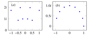
Figure 1: The figure shows the eigenvalues and the norming constant for an $8$-soliton solutions.

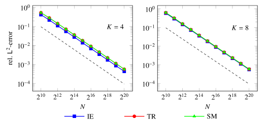
Figure 2: The figure shows the convergence analysis for the discrete Darboux transformation for $K$-soliton solutions ($K=4,8$) corresponding to the discrete spectrum defined in Sec. III with respect to the number of samples $N$. The discrete systems correspond to the implicit Euler (IE) method, the trapezoidal rule (TR) and the split-Magnus (SM) method. The dashed line depicts the $\mathop{O}(N^{-1})$ curve for reference.

III Numerical Test and Conclusion

A simple numerical test can be designed to confirm the rate of convergence of the discrete Darboux transformation derived in the earlier sections. Define

$$\bm{\theta}=\left(\frac{\pi}{3},\frac{13\pi}{30},\frac{8\pi}{15},\frac{19\pi}{30}\right),$$ (96)

and let the set of eigenvalues be $\{\exp(i\bm{\theta}),2\exp(i\bm{\theta})\}$. The corresponding norming constants are chosen as

$$b_{j}=\exp{[i(\pi/8)(j-1)]},\quad j=1,2,\ldots,8.$$ (97)

The discrete spectrum defined above is shown in Fig. 1. Let the time domain be $\Omega=[-10,10]$ and the grid be defined as $t_{n}=nh,\,n=-N/2,\ldots,N/2-1,$ where $h=20/N$. The number of samples $N$ varies within the set $\{2^{10},2^{11},\ldots,2^{20}\}$. The error in computing the $K$-soliton solutions is quantified by

$$e_{\text{rel.}}=\|q-q^{\text{num.}}\|_{\mathsf{L}^{2}(\Omega)}/\|q\|_{\mathsf{L}^{2}(\Omega)},$$ (98)

where the integrals are estimated using the trapezoidal rule. The exact solution is computed using the classical Darboux transformation. The convergence analysis for the $4$-soliton and the $8$-soliton solutions are shown in Fig. 2 which clearly indicates that rate of convergence is $\mathop{O}(N^{-1})$ for each of the methods considered.

References

- Zakharov and Shabat (1972) V. E. Zakharov and A. B. Shabat, “Exact theory of two-dimensional self-focusing and one-dimensional self-modulation of waves in nonlinear media,” Sov. Phys. JETP 34, 62–69 (1972).
- Ablowitz et al. (1974) M. J. Ablowitz, D. J. Kaup, A. C. Newell, and H. Segur, “The inverse scattering transform - Fourier analysis for nonlinear problems,” Stud. Appl. Math. 53, 249–315 (1974).
- Ablowitz and Ladik (1975) M. J. Ablowitz and J. F. Ladik, “Nonlinear differential–difference equations,” J. Math. Phys. 16, 598–603 (1975).
- Ablowitz and Ladik (1976) M. J. Ablowitz and J. F. Ladik, “Nonlinear differential–difference equations and Fourier analysis,” J. Math. Phys. 17, 1011–1018 (1976).
- Rourke (2004) D. E. Rourke, “Elementary Bäcklund transformations for a discrete Ablowitz–Ladik eigenvalue problem,” J. Phys. A: Math. Gen. 37, 2693 (2004).
- Geng (1989) X. Geng, “Darboux transformation of the discrete Ablowitz-Ladik eigenvalue problem,” Acta Math. Sci. 9, 21 – 26 (1989).
- Vaibhav (2017) V. Vaibhav, “Fast inverse nonlinear Fourier transformation using exponential one-step methods: Darboux transformation,” Phys. Rev. E 96, 063302 (2017).
- Cox and Matthews (2002) S. M. Cox and P. C. Matthews, “Exponential time differencing for stiff systems,” J. Comput. Phys. 176, 430–455 (2002).
- Vaibhav (2018a) V. Vaibhav, “Fast inverse nonlinear Fourier transform,” Phys. Rev. E 98, 013304 (2018a).
- Vaibhav (2018b) V. Vaibhav, “Higher order convergent fast nonlinear Fourier transform,” IEEE Photonics Technol. Lett. 30, 700–703 (2018b).
- Bruckstein, Levy, and Kailath (1985) A. M. Bruckstein, B. C. Levy, and T. Kailath, “Differential methods in inverse scattering,” SIAM J. Appl. Math. 45, 312–335 (1985).
- Bruckstein and Kailath (1987) A. M. Bruckstein and T. Kailath, “Inverse scattering for discrete transmission-line models,” SIAM Rev. 29, 359–389 (1987).
- Neugebauer and Meinel (1984) G. Neugebauer and R. Meinel, “General N-soliton solution of the AKNS class on arbitrary background,” Phys. Lett. A 100, 467–470 (1984).