*

Muon Ionization Cooling Experiment

RAL-P-2018-005

 

First particle-by-particle measurement of emittance in the Muon Ionization Cooling Experiment
MICE collaboration

The Muon Ionization Cooling Experiment (MICE) seeks to demonstrate the feasibility of ionization cooling, the technique by which it is proposed to cool the muon beam at a future neutrino factory or muon collider. The emittance is measured from an ensemble of muons assembled from those that pass through the experiment. A pure muon ensemble is selected using a particle-identification system that can reject efficiently both pions and electrons. The position and momentum of each muon are measured using a high-precision scintillating-fibre tracker in a 4 T solenoidal magnetic field. This paper presents the techniques used to reconstruct the phase-space distributions in the upstream tracking detector and reports the first particle-by-particle measurement of the emittance of the MICE Muon Beam as a function of muon-beam momentum.

1 Introduction

Stored muon beams have been proposed as the source of neutrinos at a neutrino factory [1, 2] and as the means to deliver multi-TeV lepton-antilepton collisions at a muon collider [3, 4]. In such facilities the muon beam is produced from the decay of pions generated by a high-power proton beam striking a target. The tertiary muon beam occupies a large volume in phase space. To optimise the muon yield for a neutrino factory, and luminosity for a muon collider, while maintaining a suitably small aperture in the muon-acceleration system requires that the muon beam be ‘cooled’ (i.e., its phase-space volume reduced) prior to acceleration. An alternative approach to the production of low-emittance muon beams through the capture of $\mu^{+}\mu^{-}$ pairs close to threshold in electron–positron annihilation has recently been proposed [5]. To realise the luminosity required for a muon collider using this scheme requires the substantial challenges presented by the accumulation and acceleration of the intense positron beam, the high-power muon-production target, and the muon-capture systems to be addressed.

A muon is short-lived, with a lifetime of 2.2 $\mu$s in its rest frame. Beam manipulation at low energy ($\leq 1$ GeV) must be carried out rapidly. Four cooling techniques are in use at particle accelerators: synchrotron-radiation cooling [6]; laser cooling [7, 8, 9]; stochastic cooling [10]; and electron cooling [11]. In each case, the time taken to cool the beam is long compared to the muon lifetime. In contrast, ionization cooling is a process that occurs on a short timescale. A muon beam passes through a material (the absorber), loses energy, and is then re-accelerated. This cools the beam efficiently with modest decay losses. Ionization cooling is therefore the technique by which it is proposed to increase the number of particles within the downstream acceptance for a neutrino factory, and the phase-space density for a muon collider [12, 13, 14]. This technique has never been demonstrated experimentally and such a demonstration is essential for the development of future high-brightness muon accelerators or intense muon facilities.

The international Muon Ionization Cooling Experiment (MICE) has been designed [15] to perform a full demonstration of transverse ionization cooling. Intensity effects are negligible for most of the cooling channels conceived for the neutrino factory or muon collider [16]. This allows the MICE experiment to record muon trajectories one particle at a time. The MICE collaboration has constructed two solenoidal spectrometers, one placed upstream, the other downstream, of the cooling cell. An ensemble of muon trajectories is assembled offline, selecting an initial distribution based on quantities measured in the upstream particle-identification detectors and upstream spectrometer. This paper describes the techniques used to reconstruct the phase-space distributions in the spectrometers. It presents the first measurement of the emittance of momentum-selected muon ensembles in the upstream spectrometer.

2 Calculation of emittance

Emittance is a key parameter in assessing the overall performance of an accelerator [17]. The luminosity achieved by a collider is inversely proportional to the emittance of the colliding beams, and therefore beams with small emittance are required.

A beam travelling through a portion of an accelerator may be described as an ensemble of particles. Consider a beam that propagates in the positive $z$ direction of a right-handed Cartesian coordinate system, $(x,y,z)$. The position of the $i^{\rm th}$ particle in the ensemble is $\mathbf{r}_{i}=(x_{i},y_{i})$ and its transverse momentum is $\mathbf{p}_{Ti}=(p_{xi},p_{yi})$; $\mathbf{r}_{i}$ and $\mathbf{p}_{Ti}$ define the coordinates of the particle in transverse phase space. The normalised transverse emittance, $\varepsilon_{N}$, of the ensemble approximates the volume occupied by the particles in four-dimensional phase space and is given by

$$\varepsilon_{N}=\frac{1}{m_{\mu}}\sqrt[4]{\det\mathcal{C}}\,,$$ (1)

where $m_{\mu}$ is the rest mass of the muon, $\mathcal{C}$ is the four-dimensional covariance matrix,

$$\mathcal{C}=\left(\begin{matrix}\sigma_{xx}&\sigma_{xp_{x}}&\sigma_{xy}&\sigma_{xp_{y}}\\ \sigma_{xp_{x}}&\sigma_{p_{x}p_{x}}&\sigma_{yp_{x}}&\sigma_{p_{x}p_{y}}\\ \sigma_{xy}&\sigma_{yp_{x}}&\sigma_{yy}&\sigma_{yp_{y}}\\ \sigma_{xp_{y}}&\sigma_{p_{x}p_{y}}&\sigma_{yp_{y}}&\sigma_{p_{y}p_{y}}\end{matrix}\right)\,,$$ (2)

and $\sigma_{\alpha\beta}$, where $\alpha,\beta=x,y,p_{x},p_{y}$, is given by

$$\sigma_{\alpha\beta}=\frac{1}{N-1}\left(\Sigma_{i}^{N}\alpha_{i}\beta_{i}-\frac{\left(\Sigma_{i}^{N}\alpha_{i}\right)\left(\Sigma_{i}^{N}\beta_{i}\right)}{N}\right)\,.$$ (3)

The MICE experiment was operated such that muons passed through the experiment one at a time. The phase-space coordinates of each muon were measured. An ensemble of muons that was representative of the muon beam was assembled using the measured coordinates. The normalised transverse emittance of the ensemble was then calculated by evaluating the sums necessary to construct the covariance matrix, $\mathcal{C}$, and using equation 1.

3 The Muon Ionization Cooling Experiment

The muons for MICE came from the decay of pions produced by an internal target dipping directly into the circulating proton beam of the ISIS synchrotron at the Rutherford Appleton Laboratory (RAL) [18, 19]. The burst of particles resulting from one target dip is referred to as a ‘spill’. A transfer line of nine quadrupoles, two dipoles and a superconducting ‘decay solenoid’ selected a momentum bite and transported the beam into the experiment [20]. The small fraction of pions that remained in the beam were rejected during analysis using the time-of-flight hodoscopes, TOF0 and TOF1, and Cherenkov counters that were installed in the MICE Muon Beam line upstream of the cooling experiment [21, 22]. A ‘diffuser’ was installed at the upstream end of the experiment to vary the initial emittance of the beam by introducing a changeable amount of tungsten and brass, which are high-$Z$ materials, into the beam path [20].

A schematic diagram of the experiment is shown in figure 1. It contained an absorber/focus-coil module sandwiched between two spectrometer-solenoid modules that provided a uniform magnetic field for momentum measurement. The focus-coil module had two separate windings that were operated with the same, or opposed, polarities. A lithium-hydride or liquid-hydrogen absorber was placed at the centre of the focus-coil module. An iron Partial Return Yoke (PRY) was installed around the experiment to contain the field produced by the solenoidal spectrometers (not shown in figure 1). The PRY was installed at a distance from the beam axis such that its effect on the trajectories of particles travelling through the experiment was negligible.

Figure 1: Schematic diagram of the MICE experiment. The red rectangles represent the coils of the spectrometer solenoids and focus-coil module. The individual coils of the spectrometer solenoids are labelled E1, C, E2, M1 and M2. The various detectors (time-of-flight hodoscopes (TOF0, TOF1) [23, 24], Cherenkov counters [25], scintillating-fibre trackers [26], KLOE-Light (KL) calorimeter [20, 27], and Electron Muon Ranger (EMR) [28, 29]) are also represented. The Partial Return Yoke (PRY) is not shown.

The emittance was measured upstream and downstream of the absorber and focus-coil module using scintillating-fibre tracking detectors [26] immersed in the solenoidal field provided by three superconducting coils E1, C, and E2. The trackers were used to reconstruct the trajectories of individual muons at the entrance and exit of the absorber. The trackers were each constructed from five planar stations of scintillating fibres, each with an active radius of 150 mm. The track parameters were reported at the nominal reference plane: the surface of the scintillating-fibre plane closest to the absorber [30]. Hall probes were installed on the tracker to measure the magnetic-field strength in situ. The instrumentation up- and downstream of the spectrometer modules was used to select a pure sample of muons. The reconstructed tracks of the selected muons were then used to measure the muon-beam emittance at the upstream and downstream tracker reference planes. The spectrometer-solenoid modules also contained two superconducting ‘matching’ coils (M1, M2) that were used to match the optics between the uniform-field region and the neighbouring focus-coil module. The MICE coordinate system is such that the $z$-axis is coincident with the beam direction, the $y$-axis points vertically upward, and the $x$-axis completes a right-handed co-ordinate system. This paper discusses the measurement of emittance using only the tracker and beam-line instrumentation upstream of the absorber. The diffuser was fully retracted for the presented data, i.e. no extra material was introduced into the centre of the beam line, so that the incident particle distribution could be assessed.

4 MICE Muon Beam line

The MICE Muon Beam line is shown schematically in figure 2. It was capable of delivering beams with normalised transverse emittance in the range $3\lesssim\varepsilon_{N}\lesssim 10$ mm and mean momentum in the range $140\lesssim p_{\mu}\lesssim 240$ MeV/$c$ with a root-mean-squared (RMS) momentum spread of $\sim$20 MeV/$c$ [20] after the diffuser (figure 1).

Pions produced by the momentary insertion of a titanium target [18, 19] into the ISIS proton beam were captured using a quadrupole triplet (Q1–3) and transported to a first dipole magnet (D1), which selected particles of a desired momentum bite into the 5 T decay solenoid (DS). Muons produced in pion decay in the DS were momentum-selected using a second dipole magnet (D2) and focused onto the diffuser by a quadrupole channel (Q4–6 and Q7–9). In positive-beam running, a borated polyethylene absorber of variable thickness was inserted into the beam just downstream of the decay solenoid to suppress the high rate of protons that were produced at the target [31].

The composition and momentum spectra of the beams delivered to MICE were determined by the interplay between the two bending magnets D1 and D2. In ‘muon mode’, D2 was set to half the current of D1, selecting backward-going muons in the pion rest frame. This produced an almost pure muon beam.

Data were taken in October 2015 in muon mode at a nominal momentum of 200 MeV/$c$, with ISIS in operation at 700 MeV. These data [32] are used here to characterise the properties of the beam accepted by the upstream solenoid with all diffuser irises withdrawn from the beam. The upstream E1-C-E2 coils in the spectrometer module were energised and produced a field of 4 T, effectively uniform across the tracking region, while all other coils were unpowered. Positively charged particles were selected due to their higher production rate in 700 MeV proton-nucleus collisions.

Figure 2: (a) Top and (b) side views of the MICE Muon Beam line, its instrumentation, and the experimental configuration. A titanium target dipped into the ISIS proton synchrotron and the resultant spill of particles was captured with a quadrupole triplet (Q1–3) and transported through momentum-selecting dipoles (D1, D2). The quadrupole triplets (Q4–6, Q7–9) transported particles to the upstream spectrometer module. The time-of-flight of particles, measured between TOF0 and TOF1, was used for particle identification.

5 Simulation

Monte Carlo simulations were used to determine the accuracy of the kinematic reconstruction, to evaluate the efficiency of the response of the scintillating-fibre tracker, and to study systematic uncertainties. A sufficient number of events were generated to ensure that statistical uncertainties from the simulations were negligible in comparison to those of the data.

The beam impinging on TOF0 was modelled using G4beamline [33]. Particles were produced at the target using a parameterised particle-production model. These particles were tracked through the MICE Muon Beam line taking into account all material in and surrounding the beam line and using realistic models of the field and apertures of the various magnets. The G4beamline simulation was tuned to reproduce the observed particle distributions at TOF0.

The MICE Analysis User Software (MAUS) [34] package was used to simulate the passage of particles from TOF0 through the remainder of the MICE Muon Beam line and through the solenoidal lattice. This simulation includes the response of the instrumentation and used the input distribution produced using G4beamline. MAUS was also used for offline reconstruction and to provide fast real-time detector reconstruction and data visualisation during MICE running. MAUS uses GEANT4 [35, 36] for beam propagation and the simulation of detector response. ROOT [37] was used for data visualisation and for data storage. The particles generated were subjected to the same trigger requirements as the data and processed by the same reconstruction programs.

6 Beam selection

Data were buffered in the front-end electronics and read out at the end of each spill [20]. For the reconstructed data presented here, the digitisation of analogue signals received from the detectors was triggered by a coincidence of signals in the PMTs serving a single scintillator slab in TOF1. Any slab in TOF1 could generate a trigger.

The following cuts were used to select muons passing through the upstream tracker:

• One reconstructed space-point in TOF0 and TOF1: Each TOF hodoscope was composed of two perpendicular planes of scintillator slabs arranged to measure the $x$ and $y$ coordinates. A space-point was formed from the intersection of hits in the $x$ and $y$ projections. Figures 3a and 3b show the hit multiplicity in TOF0 plotted against the hit multiplicity in TOF1 for reconstructed data and reconstructed Monte Carlo respectively. The sample is dominated by events with one space-point in both TOF0 and TOF1. This cut removes events in which two particles enter the experiment within the trigger window.

• Relative time-of-flight between TOF0 and TOF1, $\mathit{t_{\mathrm{rel}}}$, in the range $\mathit{1\leq t_{\mathrm{rel}}\leq 6}$ ns: The time of flight between TOF0 and TOF1, $t_{01}$, was measured relative to the mean positron time of flight, $t_{e}$. Figure 3c shows the relative time-of-flight distribution in data (black, circles) and simulation (filled histogram). All cuts other than the relative time-of-flight cut have been applied in this figure. The time-of-flight of particles relative to the mean positron time-of-flight is calculated as

  $$t_{\mathrm{rel}}=t_{01}-\left(t_{e}+\delta t_{e}\right)\,,$$

  where $\delta t_{e}$ accounts for the difference in transit time, or path length travelled, between electrons and muons in the field of the quadrupole triplets [21]. This cut removes electrons from the selected ensemble as well as a small number of pions. The data has a longer tail compared to the simulation, which is related to the imperfect simulation of the longitudinal momentum of particles in the beam (see section 7.1).

• A single track reconstructed in the upstream tracker with a track-fit $\mathit{\chi^{2}}$ satisfying $\mathit{\frac{\chi^{2}}{N_{\rm DOF}}\leq 4}$: $N_{\rm DOF}$ is the number of degrees of freedom. The distribution of $\frac{\chi^{2}}{N_{\rm DOF}}$ is shown in figure 3d. This cut removes events with poorly reconstructed tracks. Multi-track events, in which more than one particle passes through the same pixel in TOF0 and TOF1 during the trigger window, are rare and are also removed by this cut. The distribution of $\frac{\chi^{2}}{N_{\rm DOF}}$ is broader and peaked at slightly larger values in the data than in the simulation.

• Track contained within the fiducial volume of the tracker: The radius of the track measured by the tracker, $R_{\rm track}$, is required to satisfy $R_{\rm track}<150$ mm to ensure the track does not leave and then re-enter the fiducial volume. The track radius is evaluated at 1 mm intervals between the stations. If the track radius exceeds 150 mm at any of these positions, the event is rejected.

• Extrapolated track radius at the diffuser, $\mathit{R_{\rm diff}\leq 90}$ mm: Muons that pass through the annulus of the diffuser, which includes the retracted irises, lose a substantial amount of energy. Such muons may re-enter the tracking volume and be reconstructed but have properties that are no longer characteristic of the incident muon beam. The aperture radius of the diffuser mechanism (100 mm) defines the transverse acceptance of the beam injected into the experiment. Back-extrapolation of tracks to the exit of the diffuser yields a measurement of $R_{\rm diff}$ with a resolution of $\sigma_{R_{\rm diff}}=1.7$ mm. Figure 3e shows the distribution of $R_{\rm diff}$, where the difference between data and simulation lies above the accepted radius. These differences are due to approximations in modelling the outer material of the diffuser. The cut on $R_{\rm diff}$ accepts particles that passed at least $5.9\sigma_{R_{\rm diff}}$ inside the aperture limit of the diffuser.

• Particle consistent with muon hypothesis: Figure 4 shows $t_{01}$, the time-of-flight between TOF0 and TOF1, plotted as a function of $p$, the momentum reconstructed by the upstream tracking detector. Momentum is lost between TOF1 and the reference plane of the tracker in the material of the detectors. A muon that loses the most probable momentum, $\Delta p\simeq 20$ MeV/$c$, is shown as the dotted (white) line. Particles that are poorly reconstructed, or have passed through support material upstream of the tracker and have lost significant momentum, are excluded by the lower bound. The population of events above the upper bound are ascribed to the passage of pions, or mis-reconstructed muons, and are also removed from the analysis.

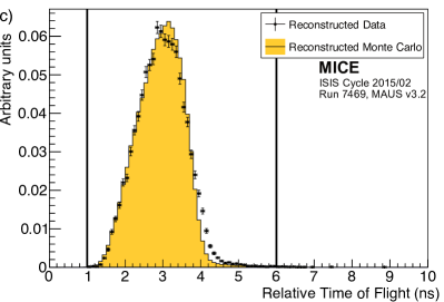
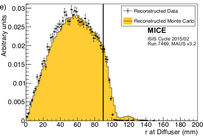
Figure 3: Distribution of the quantities that were used to select the sample used to reconstruct the emittance of the beam: a) the number of space-points in TOF0 plotted against the number of space-points in TOF1 for reconstructed data, and b) reconstructed simulation; c) distribution of the relative time-of-flight, $t_{\mathrm{rel}}$; d) distribution of $\frac{\chi^{2}}{N_{\rm DOF}}$; and e) distribution of $R_{\rm diff}$. The 1D distributions show reconstructed data as solid (black) circles and reconstructed MAUS simulation as the solid (yellow) histogram. The solid (black) lines indicate the position of the cuts made on these quantities. Events enter these plots if all cuts other than the cut under examination are passed.

A total of 24 660 events pass the cuts listed above. Table 1 shows the number of particles that survive each individual cut. Data distributions are compared to the distributions obtained using the MAUS simulation in figures 3 and 4. Despite minor disagreements, the agreement between the simulation and data is sufficiently good to give confidence that a clean sample of muons has been selected.

The expected pion contamination of the unselected ensemble of particles has been measured to be $\leq 0.4$ %[22]. Table 2 shows the number of positrons, muons, and pions in the MAUS simulation that pass all selection criteria. The criteria used to select the muon sample for the analysis presented here efficiently reject electrons and pions from the Monte Carlo sample.

Figure 4: Time of flight between TOF0 and TOF1 ($t_{01}$) plotted as a function of the muon momentum, $p$, measured in the upstream tracker. All cuts other than the muon hypothesis have been applied. Particles within the black lines are selected. The white dotted line is the trajectory of a muon that loses the most probable momentum (20 MeV/$c$) between TOF1 and the tracker in a) reconstructed data, and b) reconstructed Monte Carlo.

Table 1: The number of particles that pass each selection criterion. A total of 24 660 particles pass all of the cuts.

Cut	No. surviving particles	Cumulative surviving particles
None	53 276	53 276
One space-point in TOF0 and TOF1	37 619	37 619
Relative time of flight in range 1–6 ns	37 093	36 658
Single reconstructed track with $\frac{\chi^{2}}{N_{\rm DOF}}\leq 4$	40 110	30 132
Track within fiducial volume of tracker	52 039	29 714
Extrapolated track radius at diffuser $\leq\,90$ mm	42 592	25 310
Muon hypothesis	34 121	24 660
All	24 660	24 660

Table 2: The number of reconstructed electrons, muons, and pions at the upstream tracker that survive each cut in the Monte Carlo simulation. Application of all cuts removes almost all positrons and pions in the reconstructed Monte Carlo sample. A total of 253 504 particles pass all of the described cuts in the Monte Carlo simulation.

Cut	$e$	$\mu$	$\pi$	Total
None	14 912	432 294	1 610	463 451
One space-point in TOF0 and TOF1	11 222	353 613	1 213	376 528
Relative Time of flight in range 1–6 ns	757	369 337	1 217	379 761
Single reconstructed track with $\frac{\chi^{2}}{N_{\rm DOF}}\leq 4$	10 519	407 276	1 380	419 208
Track within fiducial volume of tracker	14 527	412 857	1 427	443 431
Tracked radius at diffuser $\leq\,90$ mm	11 753	311 076	856	334 216
Muon hypothesis (above lower limit)	3 225	362 606	411	367 340
Muon hypothesis (below upper limit)	12 464	411 283	379	424 203
Muon hypothesis (overall)	2 724	358 427	371	361 576
All	22	253 475	5	253 504

7 Results

7.1 Phase-space projections

The distributions of $x,y,p_{x},p_{y},p_{z}$, and $p=\sqrt{p^{2}_{x}+p^{2}_{y}+p^{2}_{z}}$ are shown in figure 5. The total momentum of the muons that make up the beam lie within the range $140\lesssim|p|\lesssim 260$ MeV/$c$. The results of the MAUS simulation, which are also shown in figure 5, give a reasonable description of the data. In the case of the longitudinal component of momentum, $p_{z}$, the data are peaked to slightly larger values than the simulation. The difference is small and is reflected in the distribution of the total momentum, $p$. As the simulation began with particle production from the titanium target, any difference between the simulated and observed particle distributions would be apparent in the measured longitudinal and total momentum distributions. The scale of the observed disagreement is small, and as such the simulation adequately describes the experiment. The distributions of the components of the transverse phase space ($x,p_{x},y,p_{y}$) are well described by the simulation. Normalised transverse emittance is calculated with respect to the means of the distributions (equation 2), and so is unaffected by this discrepancy.

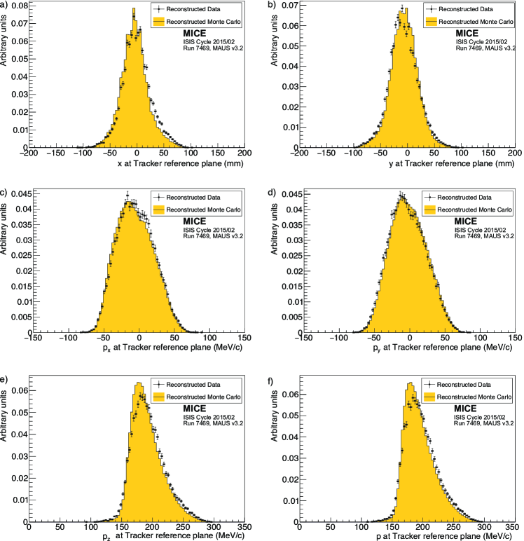
Figure 5: Position and momentum distributions of muons reconstructed at the reference surface of the upstream tracker: a) $x$, b) $y$, c) $p_{x}$, d) $p_{y}$, e) $p_{z}$, and f) $p$, the total momentum. The data are shown as the solid circles while the results of the MAUS simulation are shown as the yellow histogram.

The phase space occupied by the selected beam is shown in figure 6. The distributions are plotted at the reference surface of the upstream tracker. The beam is moderately well centred in the $(x,y)$ plane. Correlations are apparent that couple the position and momentum components in the transverse plane. The transverse position and momentum coordinates are also seen to be correlated with total momentum. The correlation in the $(x,p_{y})$ and $(y,p_{x})$ plane is due to the solenoidal field, and is of the expected order. The dispersion and chromaticity of the beam are discussed further in section 7.2.

Figure 6: Transverse phase space occupied by selected muons transported through the MICE Muon Beam line to the reference plane of the upstream tracker. a) $(x,p_{x})$, b) $(x,p_{y})$. c) $(y,p_{x})$, d) $(y,p_{y})$. e) $(x,y)$, and f) $(p_{x},p_{y})$.

7.2 Effect of dispersion, chromaticity, and binning in longitudinal momentum

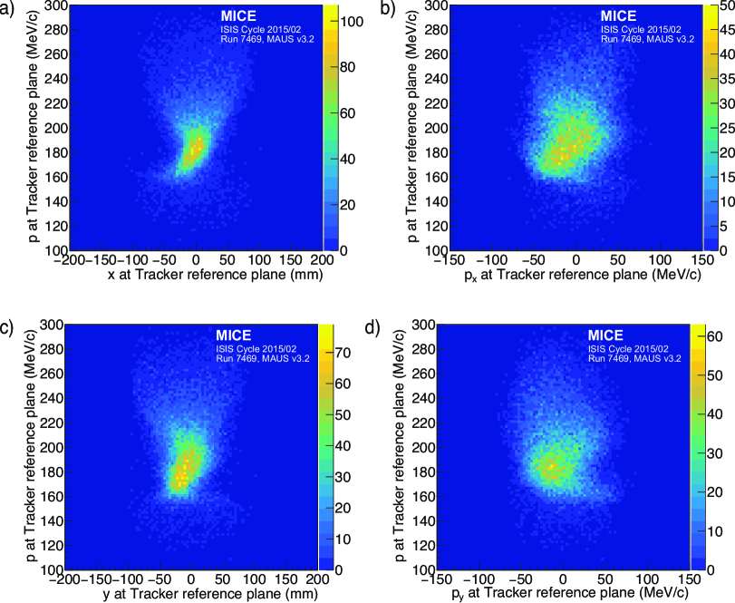
Figure 7: The effect of dispersion, the dependence of the components of transverse phase space on the momentum, $p$, is shown at the reference surface of the upstream tracker: a) $(x,p)$; b) $(p_{x},p)$; c) $(y,p)$; d) $(p_{y},p)$.

Momentum selection at D2 introduces a correlation, dispersion, between the position and momentum of particles. Figure 7 shows the transverse position and momentum with respect to the total momentum, $p$, as measured at the upstream-tracker reference plane. Correlations exist between all four transverse phase-space co-ordinates and the total momentum.

Emittance is calculated in $10$ MeV/$c$ bins of total momentum in the range $185\leq p\leq 255$ MeV/$c$. This bin size was chosen as it is commensurate with the detector resolution. Calculating the emittance in momentum increments makes the effect of the optical mismatch, or chromaticity, small compared to the statistical uncertainty. The range of $185\leq p\leq 255$ MeV/$c$ was chosen to maximise the number of particles in each bin that are not scraped by the aperture of the diffuser.

7.3 Uncertainties on Emittance Measurement

7.3.1 Statistical uncertainties

The statistical uncertainty on the emittance in each momentum bin is calculated as $\sigma_{\varepsilon}=\frac{\varepsilon}{\sqrt{2N}}$ [38, 39, 40], where $\varepsilon$ is the emittance of the ensemble of muons in the specified momentum range and $N$ is the number of muons in that ensemble. The number of events per bin varies from $\sim 4\,000$ for $p\sim 190$ MeV/$c$ to $\sim 700$ for $p\sim 250$ MeV/$c$.

7.4 Systematic uncertainties

7.4.1 Uncorrelated systematic uncertainties

Systematic uncertainties related to the beam selection were estimated by varying the cut values by an amount corresponding to the RMS resolution of the quantity in question. The emittance of the ensembles selected with the changed cut values were calculated and compared to the emittance calculated using the nominal cut values and the difference taken as the uncertainty due to changing the cut boundaries. The overall uncertainty due to beam selection is summarised in table 3. The dominant beam-selection uncertainty is in the selection of particles that successfully pass within the inner 90 mm of the diffuser aperture.

Systematic uncertainties related to possible biases in calibration constants were evaluated by varying each calibration constant by its resolution. Systematic uncertainties related to the reconstruction algorithms were evaluated using the MAUS simulation. The positive and negative deviations from the nominal emittance were added in quadrature separately to obtain the total positive and negative systematic uncertainty. Sources of correlated uncertainties are discussed below.

7.4.2 Correlated systematic uncertainties

Figure 8: The systematic bias and uncertainty on the reconstructed emittance under different magnetic field model assumptions. The bias estimate (open triangles) includes the non-uniformity bias (open squares). The variation between the models (see text) is indicated by the shaded bands.

Some systematic uncertainties are correlated with the total momentum, $p$. For example, the measured value of $p$ dictates the momentum bin to which a muon is assigned for the emittance calculation. The uncertainty on the emittance reconstructed in each bin has been evaluated by allowing the momentum of each muon to fluctuate around its measured value according to a Gaussian distribution of width equal to the measurement uncertainty on $p$. In table 3 this uncertainty is listed as ‘Binning in $p$’.

A second uncertainty that is correlated with total momentum is the uncertainty on the reconstructed $x,p_{x},y$, and $p_{y}$. The effect on the emittance was evaluated with the same procedure used to evaluate the uncertainty due to binning in total momentum. This is listed as ‘Tracker resolution’ in table 3.

Systematic uncertainties correlated with $p$ are primarily due to the differences between the model of the apparatus used in the reconstruction and the hardware actually used in the experiment. The most significant contribution arises from the magnetic field within the tracking volume. Particle tracks are reconstructed assuming a uniform solenoidal field, with no fringe-field effects. Small non-uniformities in the magnetic field in the tracking volume will result in a disagreement between the true parameters and the reconstructed values. To quantify this effect, six field models (one optimal and five additional models) were used to estimate the deviation in reconstructed emittance from the true value under realistic conditions. Three families of field model were investigated, corresponding to the three key field descriptors: field scale, field alignment, and field uniformity. The values of these descriptors that best describe the Hall-probe measurements were used to define the optimal model and the uncertainty in the descriptor values were used to determine the $1\sigma$ variations.

7.4.3 Field scale

Hall-probes located on the tracker provided measurements of the magnetic field strength within the tracking volume at known positions. An optimal field model was produced with a scale factor of 0.49 % that reproduced the Hall-probe measurements. Two additional field models were produced which used scale factors that were one standard deviation, $\pm 0.03$ %, above and below the nominal value.

7.4.4 Field alignment

A field-alignment algorithm was developed based on the determination of the orientation of the field with respect to the mechanical axis of the tracker using coaxial tracks with $p_{T}\approx 0$ [41]. The field was rotated with respect to the tracker by $1.4\pm 0.1$ mrad about the $x$-axis and $0.3\pm 0.1$ mrad about the $y$-axis. The optimal field model was created such that the simulated alignment is in agreement with the measurements. Two additional models that vary the alignment by one standard deviation were also produced.

7.4.5 Field uniformity

A COMSOL [42] model of the field was used to generate the optimal model which includes the field generated by each coil using the ‘as-built’ parameters and the partial return yoke. A simple field model was created using only the individual coil geometries to provide additional information on the effect of field uniformity on the reconstruction. The values for the simple field model were normalised to the Hall-probe measurements as for the other field models. This represents a significant deviation from the COMSOL model, but demonstrates the stability of the reconstruction with respect to changes in field uniformity, as the variation in emittance between all field models is small (less than 0.002 mm).

For each of the 5 field models, multiple 2000-muon ensembles were generated for each momentum bin. The deviation of the calculated emittance from the true emittance was found for each ensemble. The distribution of the difference between the ensemble emittance and the true emittance was assumed to be Gaussian with mean $\varepsilon$ and variance $s^{2}=\sigma^{2}+\theta^{2}$, where $\sigma$ is the statistical uncertainty and $\theta$ is an additional systematic uncertainty. The systematic bias for each momentum bin was then calculated as [43]

$$\Delta\varepsilon_{N}=\left<\varepsilon\right>-\varepsilon_{\textrm{true}}\,,$$ (4)

where $\varepsilon_{\textrm{true}}$ is the true beam emittance in that momentum bin and $\left<\varepsilon\right>$ is the mean emittance from the $N$ ensembles. The systematic uncertainty was calculated assuming that the distribution of residuals of $\varepsilon_{i}$ from the mean, $\left<\varepsilon\right>$, satisfies a $\chi^{2}$ distribution with $N-1$ degrees of freedom,

$$\chi^{2}_{N-1}=\sum_{i}^{N}\frac{(\varepsilon_{i}-\left<\varepsilon\right>)^{2}}{\sigma^{2}+\theta^{2}}\,,$$ (5)

and $\theta$ was estimated by minimising the expression $(\chi^{2}_{N-1}-(N-1))^{2}$ [43].

The uncertainty, $\theta$, was consistent with zero in all momentum bins, whereas the bias, $\Delta\varepsilon_{N}$, was found to be momentum dependent as shown in figure 8. The bias was estimated from the mean difference between the reconstructed and true emittance values using the optimal field model. The variation in the bias was calculated from the range of values reconstructed for each of the additional field models. The model representing the effects of non-uniformities in the field was considered separately due to the significance of the deviation from the optimal model.

The results show a consistent systematic bias in the reconstructed emittance of $\approx-0.015$ mm that is a function of momentum (see table 3). The absolute variation in the mean values between the models that were used was smaller than the expected statistical fluctuations, demonstrating the stability of the reconstruction across the expected variations in field alignment and scale. The effect of the non-uniformity model was larger but still demonstrates consistent reconstruction. The biases calculated from the optimal field model were used to correct the emittance values in the final calculation (Section 7.5).

Table 3: Emittance together with the statistical and systematic uncertainties and biases as a function of mean total momentum, $\langle p\rangle$.

Source	$\langle p\rangle$ (MeV/$c$)
	190	200	210	220	230	240	250
Measured emittance (mm rad)	3.40	3.65	3.69	3.65	3.69	3.62	3.31
Statistical uncertainty	$\pm$$3.8\text{\times}{10}^{-2}$	$\pm$$4.4\text{\times}{10}^{-2}$	$\pm$$5.0\text{\times}{10}^{-2}$	$\pm$$5.8\text{\times}{10}^{-2}$	$\pm$$7.0\text{\times}{10}^{-2}$	$\pm$$8.4\text{\times}{10}^{-2}$	$\pm$$9.2\text{\times}{10}^{-2}$
Beam selection:
Diffuser aperture	$\begin{subarray}{c}$4.9\text{\times}{10}^{-2}$\\ -$3.5\text{\times}{10}^{-2}$\end{subarray}$	$\begin{subarray}{c}$5.3\text{\times}{10}^{-2}$\\ $-5.1\text{\times}{10}^{-2}$\end{subarray}$	$\begin{subarray}{c}$4.9\text{\times}{10}^{-2}$\\ $-5.7\text{\times}{10}^{-2}$\end{subarray}$	$\begin{subarray}{c}$4.7\text{\times}{10}^{-2}$\\ $-5.0\text{\times}{10}^{-2}$\end{subarray}$	$\begin{subarray}{c}$4.2\text{\times}{10}^{-2}$\\ $-3.5\text{\times}{10}^{-2}$\end{subarray}$	$\begin{subarray}{c}$11.0\text{\times}{10}^{-2}$\\ $-5.0\text{\times}{10}^{-2}$\end{subarray}$	$\begin{subarray}{c}$4.4\text{\times}{10}^{-2}$\\ $-9.6\text{\times}{10}^{-2}$\end{subarray}$
$\frac{\chi^{2}}{N_{\rm DOF}}\leq 4$	$\begin{subarray}{c}$5.1\text{\times}{10}^{-3}$\\ $-4.8\text{\times}{10}^{-3}$\end{subarray}$	$\begin{subarray}{c}$2.0\text{\times}{10}^{-3}$\\ $-1.3\text{\times}{10}^{-3}$\end{subarray}$	$\begin{subarray}{c}$1.0\text{\times}{10}^{-2}$\\ $-1.8\text{\times}{10}^{-3}$\end{subarray}$	$\begin{subarray}{c}$4.1\text{\times}{10}^{-3}$\\ $-3.3\text{\times}{10}^{-3}$\end{subarray}$	$\begin{subarray}{c}$1.2\text{\times}{10}^{-3}$\\ $-2.8\text{\times}{10}^{-4}$\end{subarray}$	$\begin{subarray}{c}$5.5\text{\times}{10}^{-3}$\\ $-6.5\text{\times}{10}^{-3}$\end{subarray}$	$\begin{subarray}{c}$7.9\text{\times}{10}^{-3}$\\ $-4.7\text{\times}{10}^{-4}$\end{subarray}$
Muon hypothesis	$\begin{subarray}{c}$4.5\text{\times}{10}^{-3}$\\ $-3.2\text{\times}{10}^{-3}$\end{subarray}$	$\begin{subarray}{c}$2.2\text{\times}{10}^{-4}$\\ $-6.8\text{\times}{10}^{-3}$\end{subarray}$	$\begin{subarray}{c}$6.4\text{\times}{10}^{-3}$\\ $-8.8\text{\times}{10}^{-4}$\end{subarray}$	$\begin{subarray}{c}$3.1\text{\times}{10}^{-3}$\\ $-4.7\text{\times}{10}^{-3}$\end{subarray}$	$\begin{subarray}{c}$1.4\text{\times}{10}^{-3}$\\ $-1.1\text{\times}{10}^{-2}$\end{subarray}$	$\begin{subarray}{c}$2.6\text{\times}{10}^{-3}$\\ $-6.7\text{\times}{10}^{-2}$\end{subarray}$	$\begin{subarray}{c}$1.3\text{\times}{10}^{-3}$\\ $-4.1\text{\times}{10}^{-3}$\end{subarray}$
Beam selection (Overall)	$\begin{subarray}{c}$4.9\text{\times}{10}^{-2}$\\ $-3.6\text{\times}{10}^{-2}$\end{subarray}$	$\begin{subarray}{c}$5.3\text{\times}{10}^{-2}$\\ $-5.2\text{\times}{10}^{-2}$\end{subarray}$	$\begin{subarray}{c}$5.0\text{\times}{10}^{-2}$\\ $-5.8\text{\times}{10}^{-2}$\end{subarray}$	$\begin{subarray}{c}$4.7\text{\times}{10}^{-2}$\\ $-5.0\text{\times}{10}^{-2}$\end{subarray}$	$\begin{subarray}{c}$4.2\text{\times}{10}^{-2}$\\ $-3.9\text{\times}{10}^{-2}$\end{subarray}$	$\begin{subarray}{c}$1.1\text{\times}{10}^{-1}$\\ $-8.4\text{\times}{10}^{-2}$\end{subarray}$	$\begin{subarray}{c}$4.5\text{\times}{10}^{-2}$\\ $-9.6\text{\times}{10}^{-2}$\end{subarray}$
Binning in $p$	$\pm$1.8\text{\times}{10}^{-2}$$	$\pm$2.1\text{\times}{10}^{-2}$$	$\pm$2.3\text{\times}{10}^{-2}$$	$\pm$2.9\text{\times}{10}^{-2}$$	$\pm$3.5\text{\times}{10}^{-2}$$	$\pm$4.3\text{\times}{10}^{-2}$$	$\pm$5.2\text{\times}{10}^{-2}$$
Magnetic field misalignment
and scale:
Bias	$-1.3\text{\times}{10}^{-2}$	$-1.4\text{\times}{10}^{-2}$	$-1.5\text{\times}{10}^{-2}$	$-1.6\text{\times}{10}^{-2}$	$-1.6\text{\times}{10}^{-2}$	$-1.7\text{\times}{10}^{-2}$	$-1.6\text{\times}{10}^{-2}$
Uncertainty	$\pm$2.0\text{\times}{10}^{-4}$$	$\pm$2.9\text{\times}{10}^{-4}$$	$\pm$8.0\text{\times}{10}^{-4}$$	$\pm$4.8\text{\times}{10}^{-4}$$	$\pm$5.5\text{\times}{10}^{-4}$$	$\pm$4.8\text{\times}{10}^{-4}$$	$\pm$4.9\text{\times}{10}^{-4}$$
Tracker resolution	$\pm$1.6\text{\times}{10}^{-3}$$	$\pm$2.1\text{\times}{10}^{-3}$$	$\pm$2.8\text{\times}{10}^{-3}$$	$\pm$3.8\text{\times}{10}^{-3}$$	$\pm$5.3\text{\times}{10}^{-3}$$	$\pm$7.0\text{\times}{10}^{-3}$$	$\pm$9.5\text{\times}{10}^{-3}$$
Total systematic uncertainty	$\begin{subarray}{c}$5.2\text{\times}{10}^{-2}$\\ $-4.0\text{\times}{10}^{-2}$\end{subarray}$	$\begin{subarray}{c}$5.7\text{\times}{10}^{-2}$\\ $-5.6\text{\times}{10}^{-2}$\end{subarray}$	$\begin{subarray}{c}$5.5\text{\times}{10}^{-2}$\\ $-6.2\text{\times}{10}^{-2}$\end{subarray}$	$\begin{subarray}{c}$5.6\text{\times}{10}^{-2}$\\ $-5.8\text{\times}{10}^{-2}$\end{subarray}$	$\begin{subarray}{c}$5.5\text{\times}{10}^{-2}$\\ $-5.2\text{\times}{10}^{-2}$\end{subarray}$	$\begin{subarray}{c}$11.7\text{\times}{10}^{-2}$\\ $-9.5\text{\times}{10}^{-2}$\end{subarray}$	$\begin{subarray}{c}$6.9\text{\times}{10}^{-2}$\\ $-11.0\text{\times}{10}^{-2}$\end{subarray}$
Corrected emittance (mm rad)	3.41	3.66	3.71	3.67	3.71	3.65	3.34
Total uncertainty	$\pm 0.06$	$\pm 0.07$	$\begin{subarray}{c}+0.07\\ -0.08\end{subarray}$	$\pm 0.08$	$\pm 0.09$	$\begin{subarray}{c}+0.14\\ -0.13\end{subarray}$	$\begin{subarray}{c}+0.12\\ -0.14\end{subarray}$
Total uncertainty (%)	$\begin{subarray}{c}+1.90\\ -1.63\end{subarray}$	$\begin{subarray}{c}+1.96\\ -1.94\end{subarray}$	$\begin{subarray}{c}+2.01\\ -2.15\end{subarray}$	$\begin{subarray}{c}+2.19\\ -2.34\end{subarray}$	$\begin{subarray}{c}+2.40\\ -2.37\end{subarray}$	$\begin{subarray}{c}+3.97\\ -3.49\end{subarray}$	$\begin{subarray}{c}+3.47\\ -4.30\end{subarray}$

Figure 9: Normalised transverse emittance as a function of total momentum, $p$, for data (black, filled circle) and reconstructed Monte Carlo (red, open triangle). The inner error bars show the statistical uncertainty. The outer error bars show the quadratic sum of the statistical and systematic uncertainties.

7.5 Emittance

The normalised transverse emittance as a function of $p$ is shown in figure 9. The emittance has been corrected for the systematic bias shown in table 3. The uncertainties plotted are those summarised in table 3, where the inner bars represent the statistical uncertainty and outer bars the total uncertainty. The emittance of the measured muon ensembles (black, filled circle) is approximately flat in the range $195\leq p\leq 245$ MeV/$c$, corresponding to the design momentum of the experiment. The mean emittance in this region is $\approx 3.7$ mm. The emittance of the reconstructed Monte Carlo is consistently lower than that of the data, and therefore gives only an approximate simulation of the beam.

8 Conclusions

A first particle-by-particle measurement of the emittance of the MICE Muon Beam was made using the upstream scintillating-fibre tracking detector in a 4 T solenoidal field. A total of 24 660 muons survive the selection criteria. The position and momenta of these muons were measured at the reference plane of the upstream tracking detector. The muon sample was divided into 10 MeV/$c$ bins of total momentum, $p$, from $185$–$255$ MeV/$c$ to account for dispersion, chromaticity, and scraping in apertures upstream of the tracking detector. The emittance of the measured muon ensembles is approximately flat from $195\leq p\leq 245$ MeV/$c$ with a mean value of $\approx 3.7$ mm across this region.

The total uncertainty on this measurement ranged from $\begin{subarray}{c}+1.9\\ -1.6\end{subarray}$% to $\begin{subarray}{c}+3.5\\ -4.3\end{subarray}$%, increasing with total momentum, $p$. As $p$ increases, the number of muons in the reported ensemble decreases, increasing the statistical uncertainty. At the extremes of the momentum range, a larger proportion of the input beam distribution is scraped on the aperture of the diffuser. This contributes to an increase in systematic uncertainty at the limits of the reported momentum range. The systematic uncertainty introduced by the diffuser aperture highlights the need to study ensembles where the total momentum, $p$, is close to the design momentum of the beam line. The total systematic uncertainty on the measured emittance is larger than that on a future measurement of the ratio of emittance before and after an absorber. The measurement is sufficiently precise to demonstrate muon ionization cooling.

The technique presented here represents the first precise measurement of normalised transverse emittance on a particle-by-particle basis. This technique will be applied to muon ensembles up- and downstream of a low-$Z$ absorber, such as liquid hydrogen or lithium hydride, to measure emittance change across the absorber and thereby to study ionization cooling.

The MICE collaboration

M. Bogomilov, R. Tsenov, G. Vankova-Kirilova
Department of Atomic Physics, St. Kliment Ohridski University of Sofia, Sofia, Bulgaria

Y. Song, J. Tang
Institute of High Energy Physics, Chinese Academy of Sciences, Beijing, China

Z. Li
Sichuan University, China

R. Bertoni, M. Bonesini, F. Chignoli, R. Mazza
Sezione INFN Milano Bicocca, Dipartimento di Fisica G. Occhialini, Milano, Italy

V. Palladino
Sezione INFN Napoli and Dipartimento di Fisica, Università Federico II, Complesso Universitario di Monte S. Angelo, Napoli, Italy

A. de Bari
Sezione INFN Pavia and Dipartimento di Fisica, Pavia, Italy

D. Orestano, L. Tortora
INFN Sezione di Roma Tre and Dipartimento di Matematica e Fisica, Università Roma Tre, Italy

Y. Kuno, H. Sakamoto, A. Sato
Osaka University, Graduate School of Science, Department of Physics, Toyonaka, Osaka, Japan

S. Ishimoto
High Energy Accelerator Research Organization (KEK), Institute of Particle and Nuclear Studies, Tsukuba, Ibaraki, Japan

M. Chung, C. K. Sung
UNIST, Ulsan, Korea

F. Filthaut
Nikhef, Amsterdam, The Netherlands

D. Jokovic, D. Maletic, M. Savic
Institute of Physics, University of Belgrade, Serbia

R. Asfandiyarov, A. Blondel, F. Drielsma, Y. Karadzhov
DPNC, Section de Physique, Université de Genève, Geneva, Switzerland

G. Charnley, N. Collomb, K. Dumbell, A. Gallagher, A. Grant, S. Griffiths, T. Hartnett, B. Martlew, A. Moss, A. Muir, I. Mullacrane, A. Oates, P. Owens, G. Stokes, P. Warburton, C. White
STFC Daresbury Laboratory, Daresbury, Cheshire, UK

D. Adams, V. Bayliss, J. Boehm, T. W. Bradshaw, C. Brown, M. Courthold, C. Macwaters, A. Nichols, R. Preece, S. Ricciardi, C. Rogers, M. Tucker, T. Stanley, J. Tarrant, A. Wilson
STFC Rutherford Appleton Laboratory, Harwell Oxford, Didcot, UK

R. Bayes, J. C. Nugent, F. J. P. Soler
School of Physics and Astronomy, Kelvin Building, The University of Glasgow, Glasgow, UK

R. Gamet, P. Cooke
Department of Physics, University of Liverpool, Liverpool, UK

G. Barber, V. J. Blackmore, D. Colling, A. Dobbs, P. Dornan, C. Hunt, P.  B.  Jurj, A. Kurup, J-B. Lagrange, K. Long, J. Martyniak, S. Middleton, J. Pasternak, M. A. Uchida
Department of Physics, Blackett Laboratory, Imperial College London, London, UK

J. H. Cobb, W. Lau
Department of Physics, University of Oxford, Denys Wilkinson Building, Oxford, UK

C. N. Booth, P. Hodgson, J. Langlands, E. Overton, V. Pec, M. Robinson, P. J. Smith, S. Wilbur
Department of Physics and Astronomy, University of Sheffield, Sheffield, UK

G.  T. Chatzitheodoridis, A. J. Dick, K. Ronald, C. G. Whyte, A. R. Young
SUPA and the Department of Physics, University of Strathclyde, Glasgow, UK

S. Boyd, P. Franchini, J. R. Greis, T. Lord, C. Pidcott, I. Taylor
Department of Physics, University of Warwick, Coventry, UK

M. Ellis, R.B.S. Gardener, P. Kyberd, J. J. Nebrensky
Brunel University, Uxbridge, UK

M. Palmer, H. Witte
Brookhaven National Laboratory, NY, USA

D. Adey, A. D. Bross, D. Bowring, A. Liu, D. Neuffer, M. Popovic, P. Rubinov
Fermilab, Batavia, IL, USA

A. DeMello, S. Gourlay, D. Li, S. Prestemon, S. Virostek, M. Zisman
Lawrence Berkeley National Laboratory, Berkeley, CA, USA

B. Freemire, P. Hanlet, D. M. Kaplan, T. A. Mohayai, D. Rajaram, P. Snopok, V. Suezaki, Y. Torun
Illinois Institute of Technology, Chicago, IL, USA

L. M. Cremaldi, D. A. Sanders, D. J. Summers
University of Mississippi, Oxford, MS, USA

L. Coney , G. G. Hanson, C. Heidt, A. Klier
University of California, Riverside, CA, USA

D. Cline, X. Yang
University of California, Los Angeles, CA, USA

References

- [1] S. Geer, “Neutrino beams from muon storage rings: Characteristics and physics potential,” Phys. Rev. D57 (1998) 6989–6997, arXiv:hep-ph/9712290.
- [2] M. Apollonio et al., “Oscillation physics with a neutrino factory,” hep-ph/0210192.
- [3] D. V. Neuffer and R. B. Palmer, “A High-Energy High-Luminosity Collider,” Conf. Proc. C940627 (1995) 52–54.
- [4] R. B. Palmer, “Muon Colliders,” Rev. Accel. Sci. Tech. 7 (2014) 137–159.
- [5] M. Boscolo, M. Antonelli, O. R. Blanco-Garcia, S. Guiducci, S. Liuzzo, P. Raimondi, and F. Collamati, “Studies of a scheme for Low EMittance Muon Accelerator with production from positrons on target,” arXiv:1803.06696 [physics.acc-ph].
- [6] S. Y. Lee, Accelerator Physics (Third Edition). World Scientific Publishing Co, 2012.
- [7] S. Schröder, R. Klein, N. Boos, M. Gerhard, R. Grieser, G. Huber, A. Karafillidis, M. Krieg, N. Schmidt, T. Kühl, R. Neumann, V. Balykin, M. Grieser, D. Habs, E. Jaeschke, D. Krämer, M. Kristensen, M. Music, W. Petrich, D. Schwalm, P. Sigray, M. Steck, B. Wanner, and A. Wolf, “First laser cooling of relativistic ions in a storage ring,” Phys. Rev. Lett. 64 (Jun, 1990) 2901–2904. http://link.aps.org/doi/10.1103/PhysRevLett.64.2901.
- [8] J. S. Hangst, M. Kristensen, J. S. Nielsen, O. Poulsen, J. P. Schiffer, and P. Shi, “Laser cooling of a stored ion beam to 1 mK,” Phys. Rev. Lett. 67 (Sep, 1991) 1238–1241. http://link.aps.org/doi/10.1103/PhysRevLett.67.1238.
- [9] P. J. Channell, “Laser cooling of heavy ion beams,” Journal of Applied Physics 52 no. 6, (1981) 3791–3793, http://dx.doi.org/10.1063/1.329218. http://dx.doi.org/10.1063/1.329218.
- [10] J. Marriner, “Stochastic cooling overview,” Nucl. Instrum. Meth. A532 (2004) 11–18, arXiv:physics/0308044 [physics].
- [11] V. V. Parkhomchuk and A. N. Skrinsky, “Electron cooling: 35 years of development,” Physics-Uspekhi 43 no. 5, (2000) 433–452. http://stacks.iop.org/1063-7869/43/i=5/a=R01.
- [12] A. N. Skrinsky and V. V. Parkhomchuk, “Cooling Methods for Beams of Charged Particles. (In Russian),” Sov. J. Part. Nucl. 12 (1981) 223–247. [Fiz. Elem. Chast. Atom. Yadra12,557(1981)].
- [13] D. Neuffer, “Principles and Applications of Muon Cooling,” Conf.Proc. C830811 (1983) 481.
- [14] D. Neuffer, “Principles and Applications of Muon Cooling,” Part. Accel. 14 (1983) 75–90.
- [15] The MICE collaboration, “INTERNATIONAL MUON IONIZATION COOLING EXPERIMENT.” http://mice.iit.edu.
- [16] ISS Accelerator Working Group Collaboration, M. Apollonio et al., “Accelerator design concept for future neutrino facilities,” JINST 4 (2009) P07001, arXiv:0802.4023 [physics.acc-ph].
- [17] J. B. Rosenzweig, Fundamentals of Beam Physics. Oxford University Press, 2003.
- [18] C. N. Booth et al., “The design, construction and performance of the MICE target,” JINST 8 (2013) P03006, arXiv:1211.6343 [physics.ins-det].
- [19] C. N. Booth et al., “The design and performance of an improved target for MICE,” JINST 11 no. 05, (2016) P05006, arXiv:1603.07143 [physics.ins-det].
- [20] MICE Collaboration, M. Bogomilov et al., “The MICE Muon Beam on ISIS and the beam-line instrumentation of the Muon Ionization Cooling Experiment,” JINST 7 (2012) P05009, arXiv:1203.4089 [physics.acc-ph].
- [21] MICE Collaboration, D. Adams et al., “Characterisation of the muon beams for the Muon Ionisation Cooling Experiment,” Eur. Phys. J. C73 no. 10, (2013) 2582, arXiv:1306.1509 [physics.acc-ph].
- [22] MICE Collaboration, M. Bogomilov et al., “Pion contamination in the MICE muon beam,” JINST 11 no. 03, (2016) P03001, arXiv:1511.00556 [physics.ins-det].
- [23] MICE Collaboration, R. Bertoni et al., “The design and commissioning of the MICE upstream time-of-flight system,” Nucl.Instrum.Meth. A615 (2010) 14–26, arXiv:1001.4426 [physics.ins-det].
- [24] R. Bertoni, M. Bonesini, A. de Bari, G. Cecchet, Y. Karadzhov, and R. Mazza, “The construction of the MICE TOF2 detector.” http://mice.iit.edu/micenotes/public/pdf/MICE0286/MICE0286.pdf, 2010.
- [25] L. Cremaldi, D. A. Sanders, P. Sonnek, D. J. Summers, and J. Reidy, Jr, “A Cherenkov Radiation Detector with High Density Aerogels,” IEEE Trans. Nucl. Sci. 56 (2009) 1475–1478, arXiv:0905.3411 [physics.ins-det].
- [26] M. Ellis et al., “The design, construction and performance of the MICE scintillating fibre trackers,” Nucl. Instrum. Meth. A659 (2011) 136–153, arXiv:1005.3491 [physics.ins-det].
- [27] F. Ambrosino et al., “Calibration and performances of the KLOE calorimeter,” Nucl. Instrum. Meth. A598 (2009) 239–243.
- [28] R. Asfandiyarov et al., “The design and construction of the MICE Electron-Muon Ranger,” JINST 11 no. 10, (2016) T10007, arXiv:1607.04955 [physics.ins-det].
- [29] MICE Collaboration, D. Adams et al., “Electron-Muon Ranger: performance in the MICE Muon Beam,” JINST 10 no. 12, (2015) P12012, arXiv:1510.08306 [physics.ins-det].
- [30] A. Dobbs, C. Hunt, K. Long, E. Santos, M. A. Uchida, P. Kyberd, C. Heidt, S. Blot, and E. Overton, “The reconstruction software for the MICE scintillating fibre trackers,” JINST 11 no. 12, (2016) T12001, arXiv:1610.05161 [physics.ins-det].
- [31] S. Blot, “Proton Contamination Studies in the MICE Muon Beam Line,” Proceedings 2nd International Particle Accelerator Conference (IPAC 11) 4-9 September 2011, San Sebastian, Spain (2011) .
- [32] The MICE Collaboration, “The MICE RAW Data.” doi:10.17633/rd.brunel.3179644. MICE/Step4/07000/07469.tar.
- [33] T. Roberts et al., “G4beamline; a “Swiss Army Knife” for Geant4, optimized for simulating beamlines.” http://public.muonsinc.com/Projects/G4beamline.aspx.
- [34] D. Rajaram and C. Rogers, “The mice offline computing capabilities.” http://mice.iit.edu/micenotes/public/pdf/MICE0439/MICE0439.pdf, 2014. MICE Note 439.
- [35] GEANT4 Collaboration, S. Agostinelli et al., “Geant4: A simulation toolkit,” Nuclear Instruments and Methods in Physics Research A 506 (2003) 250–303.
- [36] J. Allison et al., “Geant4 developments and applications,” IEEE Trans. Nucl. Sci. 53 (2006) 270–278.
- [37] R. Brun and F. Rademakers, “ROOT: An object oriented data analysis framework,” Nucl. Instrum. Meth. A389 (1997) 81–86.
- [38] J. Cobb, “Statistical Errors on Emittance Measurements.” http://mice.iit.edu/micenotes/public/pdf/MICE341/MICE268.pdf, 2009.
- [39] J. Cobb, “Statistical Errors on Emittance and Optical Functions.” http://mice.iit.edu/micenotes/public/pdf/MICE341/MICE341.pdf, 2011.
- [40] J. H. Cobb, “Statistical errors on emittance.” Private communication, 2015.
- [41] C. Hunt, “Private communication,”.
- [42] HTTP://WWW.COMSOL.COM/.
- [43] L. Lyons, “On estimating systematic errors from repeated measurements,” Journal of Physics A: Mathematical and General 25 no. 7, (1992) 1967. http://stacks.iop.org/0305-4470/25/i=7/a=035.