Hamilton-Green Solver for the Forward and Adjoint Problems in Photoacoustic Tomography

Abstract

The majority of the solvers for the acoustic problem in Photoacoustic Tomography (PAT) rely on full solution of the wave equation, which makes them less suitable for real-time and dynamic applications where only partial data is available. This is in contrast to other tomographic modalities, e.g. X-ray tomography, where partial data implies partial cost for the application of the forward and adjoint operators. In this work we present a novel solver for the forward and adjoint wave equations for the acoustic problem in PAT. We term the proposed solver Hamilton-Green as it approximates the fundamental solution to the respective wave equation along the trajectories of the Hamiltonian system resulting from the high frequency asymptotic approximate solution for the wave equation. This approach is flexible and scalable in the sense that it allows computing the solution for each sensor independently at a fraction of the cost of the full wave solution. The theoretical foundations of our approach are rooted in results available in seismics and ocean acoustics. To demonstrate the feasibility of our approach we present results for 2D domains with homogeneous and heterogeneous sound speeds and evaluate them against a full wave solution obtained with a pseudospectral finite difference method implemented in the k-Wave toolbox [70].

1 Photoacoustic tomography

Photoacoustic tomography (PAT) is a hybrid imaging technique based on the photoacoustic effect. In PAT, the biological tissue is irradiated with a laser pulse [78, 38]. Part of the energy of this pulse is absorbed in the form of heat, which is then released through thermoelastic expansion and emission of an ultrasonic wave. This wave propagates outwards, where a set of detectors placed at the boundary of the tissue records the ultrasonic pressure over time. This data is then used to reconstruct the initial pressure (PAT image). The main advantage of this modality is its ability to simultaneously obtain high spatial resolution of the ultrasonic wave and the high contrast of the optical absorption of the laser pulse. To make PAT quantitative requires a solution of a coupled acoustic and optical problem, where the initial acoustic pressure constitutes the “interior data” for the optical problem [23]. In this work we focus on the acoustic problem.

1.1 Acoustic propagation in PAT

The forward problem in PAT is modeled by the initial value problem for the wave equation in free space $\mathbb{R}^{d}$ see e.g.  [38, 4]

$$\square^{2}u(t,x):=\frac{1}{c^{2}(x)}\frac{\partial^{2}u(t,x)}{\partial t^{2}}-\Delta u(t,x) =0, (t,x)\in(0,\infty)\times\mathbb{R}^{d},$$ (1a)

$$u_{t}(0,x) =0, x\in\mathbb{R}^{d},$$ (1b)

$$u(0,x) =u_{0}(x), x\in\mathbb{R}^{d},$$ (1c)

where $c(x)\in\mathcal{C}^{\infty}(\mathbb{R}^{d})$ denotes the sound speed in $\mathbb{R}^{d}$. Reconstruction of the PAT image amounts to recovery of the initial pressure $u(0,x)=u_{0}(x)$ from pressure over time measurements at a set of ideal (isotropic and point-like) detectors $\Gamma=\{x_{0}^{m}\in\operatorname{\mathbb{R}}^{d},\;m=1,\dots,M\}$. The detectors are typically placed on the boundary of the object, covering the boundary fully or, more frequently, in part, the latter scenario potentially resulting in a limited view problem. Other factors like limited propagation time or trapping sound speed may also result in incomplete data. We denote the data obtained at the sensors over a finite measuring time $T>0$ with

$$g(t,y)=u(t,y),\quad(t,y)\in(0,T)\times\Gamma.$$ (2)

We define the forward operator $\mathcal{P}$ for PAT with sensors placed on $\Gamma$ and the measurement time $T$ as

$$\mathcal{P}:\mathcal{C}_{0}^{\infty}(\operatorname{\mathbb{R}}^{d}) \longrightarrow\mathcal{C}_{0}^{\infty}(0,T)\times\Gamma$$

$$u_{0}(x) \longmapsto\omega(t)g(t,y),$$

with $g(t,y)$ given by (2) and an aperture function $\omega(t)\in C^{\infty}_{0}(0,T)$ which applies a smooth cut off to the measurement time. The corresponding adjoint operator $\mathcal{P}^{*}$ is defined as

$$\mathcal{P}^{*}:\mathcal{C}_{0}^{\infty}(0,T)\times\Gamma \longrightarrow\mathcal{C}_{0}^{\infty}(\operatorname{\mathbb{R}}^{d})$$

$$g(t,y) \longmapsto v(x,T),$$

where $v$ is the solution to the wave equation with a time varying source supported on $(0,T)\times\Gamma$

$$\square^{2}v(t,x) =\sum_{m=1}^{M}\frac{\partial}{\partial t}\Big{(}g(T-t,x_{0}^{m})\,\omega(T-t)\Big{)}\delta(x-x_{0}^{m}),\quad (t,x)\in(0,T)\times\operatorname{\mathbb{R}}^{d},$$ (3a)

$$v_{t}(0,x) =0, x\in\mathbb{R}^{d},$$ (3b)

$$v(0,x) =0, x\in\mathbb{R}^{d},$$ (3c)

evaluated at the time $t=T$, $v(T,x)$ [4, 8]. Thus, in the adjoint problem the time reversed sensor measurements $g(T-t,x_{0}^{m})\,\omega(T-t),\,m=1,\dots,M$ act as time dependent point mass sources. In contrast, a popular technique for PAT inversion known as time reversal consists of enforcing the same time reversed measurements $g(T-t,x_{0}^{m})\,\omega(T-t),\,m=1,\dots,M$ as constraints, see e.g. [38, 68], and yields an approximate-inverse operator to $\mathcal{P}$ [32, 77]. The iterated variant of time reversal proposed in [57] effectively restores partially visible singularities which arise in limited view problems (e.g. trapping sound speed, limited time, limited angle). However, when the measured data is sparse, i.e. relatively few sensors are used, we increasingly encounter invisible singularities. Variational methods provide a simple way of incorporating prior knowledge to fill in the missing information in the data. Moreover, the adjoint operator to a sparse data problem can be directly obtained and used in the framework of variational methods with readily available convergence results. Finally, we would like to remark that we altered the functional framework introduced in [4] to suit the proposed ray based approach. The adjoint operator from [4] follows analogously where all the spatial integrals are evaluated in the sense of the definition of the Green’s function

$$\square^{2}G(t,x\mid t_{0},x_{0})=\delta(x-x_{0})\,\delta(t-t_{0}),$$

which is the framework we adapt in this paper.

1.2 Motivation

The complexity of the full wave solvers such as [35, 31] is independent from the number of sensors. For instance, for the pseudospectral finite difference solver on a cube-shaped domain of size $n^{3}$ we have a complexity of $\mathcal{O}(n^{4}\log n)$. The analogous scenario for the here proposed Hamilton-Green (HG) solver corresponds to the complete data case (with some abuse of notation as the sensor is finite) i.e. collecting $n^{2}$ measurements on one side of the cube, which results in the complexity of $\mathcal{O}(n^{5})$. Thus, at the first glance, our new method has a worse theoretical complexity than the existing full wave solvers. However, the Hamilton-Green solver also offers a number of advantages with respect to the full wave solvers which could make it competitive in scenarios with e.g. incomplete / sparse data, various region of interest problems and in conjunction with ultrasound tomography:

• Solution for each sensor is computed independently at a much lower cost, i.e. $\mathcal{O}(n^{3})$, than the full wave solution;

• In contrast to the finite difference or pseudospectral solvers, it can take advantage of irregular or multiscale grids;

• The solution can be computed on a part of the domain (a region of interest) at a largely reduced computational cost;

• The coupling of the homogeneous and inhomogeneous parts of the domain is inherent and efficiently accomplished via the step size choice;

• The Hamiltonian system underlying the trajectories computed by the Hamilton-Green solver is the one of the transmission ultrasound problem, rendering the PAT solution essentially free when coupled with ultrasound tomography.

Below we discuss a few scenarios which could benefit from the aforementioned advantages of the flexible ray based Hamilton-Green solver.

1.2.1 Joint Photoacoustic Tomography and Ultrasound Tomography Reconstruction

The quality of the PAT reconstruction hinges upon the accurate knowledge of the speed of sound in the domain. In the absence of sound speed measurements, there are two commonly taken approaches: i) assume the sound speed homogeneous and potentially fit its value via optimization; ii) deduce an inhomogeneous sound speed model from a priori information obtained from another non-acoustic modality (e.g. MRI as in [41]). The first approach hits its limitations when the inhomogeneity becomes pronounced, which occurs even in soft tissue, with differences up to 10% between different tissue types [44]. Assuming sound speed difference as in [44], imaging to 7 [cm] depth in breast disregarding the inhomogeneity between the fat and muscle, will result in an aberration on the order of mm and cause artefacts in the reconstruction. The second needs an extra scan which is potentially expensive, time consuming, requires registration of the images and the conversion of the other contrast to speed of sound is potentially difficult to justify. Therefore, recently there has been an interest in developing integrated ultrasound (US) / PAT scanners, capable of simultaneous acquisition of the US and PAT data and hence providing a registered set of measurements from which both the speed of sound and PAT image can be reconstructed e.g. [45, 46]. As the forward solve for the complete data transmission US problem requires solution of $\mathcal{O}(n^{2})$ full wave problems, the standard approach is to settle for the time of travel tomography i.e. first time of arrival e.g. [39, 25]. The Hamiltonian system underlying the bent ray tomography approaches such as [39, 25] is the same as the one used in Hamilton-Green PAT solver thus the PAT solution can be obtained essentially for “free” when solving the transmission US problem.

1.2.2 Region of Interest

The advances in the scanner hardware led to miniature endoscopic devices which can be deployed to guide surgical intervention such as e.g. the separation of the twin fetuses involving separation of veins in the placenta. In this case, the probe can be at a substantial distance from the target. This region is usually filled with a clear fluid. Furthermore, the measurements have to be acquired almost instantaneously. The region of interest tomography, to the best of our knowledge, has not been widely considered in the context of PAT. The existing full wave solvers cannot take advantage of this scenario as the wave has to be propagated through the entire domain containing the region of interest and all the sensors. On the other hand, the Hamilton-Green solver is inherently flexible and it is sufficient to restrict the propagation domain for each sensor to this sensor and the region of interest. Furthermore, as the clear fluid region can be assumed to have a homogeneous sound speed, and hence in the fluid the rays are straight lines, such a hybrid problem can be efficiently handled by simply increasing the time step in this region without deteriorating the quality of the solution.

1.2.3 Stochastic Methods and Subsampled Data

The data acquisition time in PAT presents a bottleneck in pre- and clinical environment. Hence the recent interest in studying subsampling schemes and compressed sensing to reduce the acquisition time. The computational cost of the full wave solvers is nearly independent of the number of sensors, while the cost of Hamilton-Green solver scales linearly with the number of sensors. Furthermore, stochastic methods have been shown to outperform their deterministic counterparts in applications such as PET [26, 20]. Stochastic methods use partial operators i.e. a subset of the sensors in each iteration and so are particularly well suited for the Hamilton-Green solver.

1.3 Contribution

The main theoretical contribution of this paper is a new way to construct an approximation to the solution of the time-domain wave equation which arises in forward and adjoint problems in PAT. We term our solver Hamilton-Green (HG), as it effectively approximates the time derivative of the unknown Green’s function of the underlying acoustic problem along the trajectories of the Hamiltonian system resulting from the high frequency asymptotic approximation to the solution of the wave equation. The bulk of the paper is devoted to establishing the mathematical foundations of the proposed Hamilton-Green solver. The main building blocks of the solver are derived from methods used in seismic and underwater acoustics, including the computation of phase and amplitude along the rays.

Based on this approximation we develop a novel acoustic solver for the forward and adjoint PAT problems for homogeneous and heterogeneous sound speeds. The proposed method is inherently ray based which enables evaluation of partial forward/adjoint operators (for each sensor or even each ray) at a fractional cost which is not possible with full-wave solvers and is a common and desirable feature of tomographic problems exploited by many algebraic reconstruction methods.

We discuss the approximation error of the Hamilton-Green solver for the forward and adjoint problems for PAT and support our conclusions with 2D examples in domains with homogeneous and heterogeneous sounds speeds. We compare our results to full-wave solution obtained with a pseudo-spectral finite difference method implemented in k-Wave, a well established and widely used toolbox for biomedical PAT and ultrasonic simulations.

We consider full-data problems which, as alluded to in section 1.2, while native to the full-wave solvers are not a realistic deployment scenario for our HG solver. However, we stress that our purpose here is not to compete with the full-wave solver in this context, nor to produce PAT image reconstruction, but to evaluate the impact of the approximation underlying the HG solver on both the forward and the adjoint problems. This is also the reason for restricting ourselves to 2D domains which allow for a better visualization.

In future work, the HG solver will be deployed in a number of realistic 3D scenarios which can benefit from the additional flexibility it offers.

1.4 Outline

The remainder of this paper is organized as follows. In section 2 we recall the high frequency approximation to the solution of the wave equation including the equations for the phase, the amplitude and two methods for computation of the Jacobian of the change of coordinates between the Cartesian and ray based coordinates (which corresponds to the inverse ray density). Furthermore, we derive expressions for the reversed quantities needed by the adjoint Hamilton-Green solver. Section 3 constitutes the core of the paper where we introduce the novel Hamilton-Green acoustic solver for the forward and adjoint problems in PAT. In Section 4 we analyse the error of the forward and adjoint Hamilton-Green solver. In section 5 we report simulations for both the forward and the adjoint problems. We illustrate HG convergence in homogeneous case, and evaluate HG error in inhomogeneous case against solutions obtained with the first order finite difference pseudo-spectral method implemented in k-Wave toolbox. Section 6 summarizes the contributions and conclusions of the paper and provides outlook on future research. Technical details of the solver pertaining mapping between Cartesian and ray based grids and Green’s function derivative approximation are postponed to A. A case study of the effect of caustics on HG solver on an acoustic lens example is provided in B.

2 High frequency approximate solution to the wave equation

We consider the linear scalar wave equation

$$u_{tt}-c^{2}(x)\Delta u=0,\quad(t,x)\in(0,\infty)\times\mathbb{R}^{d},$$ (4)

with $d=2,3$ and appropriate initial / boundary conditions to be specified later, where $c(x)$ is the speed of the wave in the medium. In some scenarios, the initial/boundary/source conditions induce relatively high (with respect to the size of the domain) essential frequencies [28] in the propagating waves. Accurate resolution of such high frequencies would require correspondingly fine discretization, rendering the problem computationally infeasible.

In the high frequency limit $\omega\rightarrow\infty$, one can consider the following approximation to (4). Let $u$ admit a series expansion of the form

$$u(t,x)=e^{i\omega\phi(t,x)}\sum_{k=0}^{\infty}A_{k}(t,x)(i\omega)^{-k},$$ (5)

where $\phi(t,x)$ is the phase, $A_{k}$ the coefficients of the amplitude and $\omega$ the frequency of the oscillating wave. In this representation we expect the phase $\phi$ and the amplitude coefficients $A_{k}$ to vary at a much lower temporal and spatial rate than the wave field $u$ since they are independent of $\omega$.

The geometrical optics equations are obtained by substituting the WKB expansion (5) into the wave equation (4) and equating terms of the same order to ensure that (4) holds down to $\mathcal{O}(\omega)$: terms $\mathcal{O}(\omega^{2})$ result in the eikonal equation, while terms $\mathcal{O}(\omega^{1})$ result in the transport equation.

The literature on solution of the geometrical optics equations is rich, thus the following list is necessarily incomplete. We particularly mention Beylkin’s seminal work on Fourier integral operators [9], phase-space methods for solution of eikonal equation with multi-valued phases [11, 21, 30, 27] and methods that solve for both the multi-valued phases and amplitudes [55, 56, 57] and finally ray tracing methods which solve the Hamiltonian system and the transport equation [73, 75]. Our solver is based on ray tracing approach, which has immediate parallels to other tomographic modalities, most prominently X-ray computed tomography, and has been studied extensively both theoretically and numerically, in particular in the context of seismic imaging [60, 18, 72] and ocean acoustics [37, 54].

The immediate role of the ray equations in our approach is as means to reparametrisation of the domain $\Omega\subset\operatorname{\mathbb{R}}^{d}$. Therefore we assume a fully implicit time dependence of the amplitude and phase, i.e. solely through the time dependence of the trajectory $x(t)$

$$u(t,x(t))=A(x(t))\exp^{i\omega\phi(x(t))}$$

and solve the frequency domain version of the eikonal and transport equations.

2.1 Phase

The frequency domain version of the eikonal equation reads

$$\|\nabla\phi\|=1/c=\eta,$$ (6)

where $\eta(x)=1/c(x)$ is the slowness of the medium. Following the construction in [63], we introduce the Hamiltonian $H(x,p)=c(x)\|p\|$ defined in the phase space $\mathbb{R}^{d}\times\mathbb{R}^{d}$ of double the dimensionality of the ambient space, $d$. Let $(x(t),p(t))$ be a bicharacteristic pair associated with this Hamiltonian. The Hamiltonian $H$ is constant along these bicharacteristics and is set to the initial value $H(x_{0},p_{0})=1$, which corresponds to $\|p\|=\eta$. Therefore we have

$$\dfrac{\textrm{d}x}{\textrm{d}t}=\nabla_{p}H(x,p)=\dfrac{p}{\eta^{2}}, x(0)=x_{0},$$ (7a)

$$\dfrac{\textrm{d}p}{\textrm{d}t}=-\nabla_{x}H(x,p)=\dfrac{\nabla\eta}{\eta}, p(0)=p_{0},\qquad\|p_{0}\|=\eta(x_{0}),$$ (7b)

where $(x(0),p(0))=(x_{0},p_{0})$ are the initial conditions for the Hamiltonian system (7). The point $x_{0}\in\mathbb{R}^{d}$ is the origin of the ray and should be chosen on a non-characteristic hypersurface $S\subset\mathbb{R}^{d}$.

Method of characteristics

Consider $\phi(x)$ smooth such that

$$H(x,\nabla\phi(x))=1.$$ (8)

Due to the uniqueness of the solution of (7), applying the method of characteristics we find that $(x(t),\nabla\phi(x(t)))$ is a bicharacteristic pair of $H$ with $p(t)=\nabla\phi(x(t))$. This pair can be interpreted as follows: $x(t)$ represents the trajectory in the domain, while the slowness vector $p(t)$ is the direction of propagation at each point along that trajectory. Furthermore, for $\phi(t,x)=\phi(x(t))$ the eikonal equation (6) implies a linear relation between the time and phase

$$\phi(x(t))=\phi(x_{0})+t.$$ (9)

The independence of bicharacteristic pairs (corresponding to different initial conditions for the bicharacteristic system (7)) naturally accommodates multiple phase solutions, in contrast to the inherently single phased viscosity solution (first time of arrival). The system of ODEs (7) is numerically solved using a 2nd order Runge-Kutta method. The details of the interpolation between the Cartesian and ray based grids are given in A.

2.2 Amplitude

To compute the amplitude we solve the frequency domain version of the transport equation

$$2\nabla\phi\cdot\nabla A+\Delta\phi A=0.$$ (10)

The solution of the first order equation (10) for the bicharacteristic pair $(x(t;x_{0}),p(t;p_{0}))$ at a point $x(t;x_{0})$ can be explicitly written as

$$A(x(t;x_{0}))=A(x_{0})\frac{\eta(x_{0})}{\eta(x(t;x_{0}))}\sqrt{\frac{q(0;x_{0})}{q(t;x_{0})}},$$ (11)

where $q$ is the determinant of the Jacobian $J$ of $x$ with respect to the initial data,

$$q(t;x_{0})=\det J:=\det D_{x_{0}}x(t;x_{0})=\det\left(\cfrac{\partial x(t;x_{0})}{\partial x_{0,i}}\right).$$ (12)

2.3 Jacobian determinant

For completeness we describe two methods for numerical evaluation of the determinant of the Jacobian, $q$, along the ray trajectory [28, 18]. We restrict our presentation to 2D as 3D follows analogously.

ODE method

The time evolution of the determinant $q$ can be computed solving the ODE system obtained by differentiating the Hamiltonian with respect to the initial conditions [28] and changing the order of the differentiation

$$\frac{\textrm{d}}{\textrm{d}t}\begin{pmatrix}D_{x_{0}}x\\ D_{x_{0}}p\end{pmatrix}=\begin{pmatrix}D^{2}_{px}H&D^{2}_{pp}H\\ -D^{2}_{xx}H&-(D^{2}_{px}H)^{T}\end{pmatrix}\begin{pmatrix}D_{x_{0}}x\\ D_{x_{0}}p\end{pmatrix}$$ (13)

with the initial conditions

$$D_{x_{0}}x(0;x_{0})=I,\quad D_{x_{0}}p(0;x_{0})=D^{2}\phi(x_{0}).$$ (14)

For this $t$ parametrization of the Hamiltonian, $H=c(x)\|p\|$, the entries of the system matrix (13) are

$$D^{2}_{px}H=c\left(p\nabla^{T}c\right),\qquad D^{2}_{xx}H=cD^{2}c,\qquad D^{2}_{pp}H=c^{2}\left[I-c^{2}(pp^{T})\right].$$

It remains to specify the second initial condition, $D^{2}\phi(x_{0})$. Assuming $c$ to be constant in a neighborhood of $x_{S}$, the origin of the ray or shooting point, results in an out-propagating spherical wave (phase). Setting $\phi(x_{S})=0$ we have

$$\phi(x)=\frac{\|x-x_{S}\|}{c}.$$

Furthermore, without loss of generality choosing the wave centered at the origin $x_{S}=(0,0)^{T}$ we obtain

$$\phi(x)=\frac{\|x\|}{c}=\frac{\sqrt{x_{1}^{2}+x_{2}^{2}}}{c},$$ (15)

with $x=(x_{1},x_{2})^{T}$ the Cartesian coordinates of $x$. The Hessian of (15)

$$D^{2}(\phi(x))=\frac{1}{c(x_{1}^{2}+x_{2}^{2})^{3/2}}\begin{pmatrix}x_{2}^{2}&-x_{1}x_{2}\\ -x_{1}x_{2}&x_{1}^{2}\end{pmatrix}$$

has a singularity at the shooting point $x_{S}$. To circumvent this issue we assume that the initial conditions are evaluated at a nearby point $x_{0}$ further down the ray. To be precise, the initial point $x_{0}$ at a distance $\Delta x$ in the shooting direction $p_{0}$ (see figure 1)

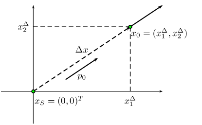
Fig. 1: The relation of the origin (shooting point) of the ray $x_{S}$ to its initial point $x_{0}$ as used to calculate the initial conditions for the ODE system (14).

$$x_{0}=\Delta x\dfrac{p_{0}}{\|p_{0}\|}=\begin{pmatrix}x_{1}^{\Delta}\\ x_{2}^{\Delta}\end{pmatrix}.$$ (16)

The Hessian at $x_{0}$

$$D^{2}\phi(x_{0})=\frac{1}{c((x^{\Delta}_{1})^{2}+(x^{\Delta}_{2})^{2})^{3/2}}\begin{pmatrix}(x^{\Delta}_{2})^{2}&-x^{\Delta}_{1}x^{\Delta}_{2}\\ -x^{\Delta}_{1}x^{\Delta}_{2}&(x^{\Delta}_{1})^{2}\end{pmatrix}.$$

is not singular but it depends on the initial point $x_{0}$ and hence implicitly on $\Delta x$, the distance from $x_{0}$ to the origin of the ray, $x_{S}$.

Proximal ray method

Inspired by an analogous construction in [18], we use a nearby ray to construct a finite difference approximation to the Jacobian $J$.

Let $\{\theta,\tau\}$ be a local coordinate system anchored at the initial point $x(0)=x_{0}$ of the ray $x(\tau)$, with $\theta$ the shooting angle and $\tau$ the parameter along the ray. We can write the Jacobian with respect to the initial conditions $x_{0}$ as

$$J_{\tau}(x)=\begin{pmatrix}\dfrac{\partial x}{\partial\theta}&\dfrac{\partial x}{\partial\tau}\end{pmatrix}$$

and approximate the derivatives with forward finite differences

$$\dfrac{\partial x(\tau,p_{0};x_{0})}{\partial\theta}\approx\dfrac{x(\tau,p_{0}^{\theta};x_{0})-x(\tau,p_{0};x_{0})}{\Delta\theta},$$

$$\dfrac{\partial x(\tau,p_{0};x_{0})}{\partial\tau}\approx\dfrac{x(\tau+\Delta\tau,p_{0};x_{0})-x(\tau,p_{0};x_{0})}{\Delta\tau}.$$

Here $x(\tau,p_{0};x_{0})$ denotes the main ray, $x(\tau,p_{0}^{\theta};x_{0})$ an auxiliary ray shot at the angle $p_{0}^{\theta}=p_{0}+\Delta\theta$ and $\Delta\tau$ is the step length along the ray (chosen equal to the step length used while solving for the trajectories). With this notation, we have the determinant of the Jacobian $q$ [18]

$$q_{\tau}(\tau;x_{0})=\begin{vmatrix}\dfrac{x(\tau,p_{0}^{\theta};x_{0})-x(\tau,p_{0};x_{0})}{\Delta\theta}&\dfrac{x(\tau+\Delta\tau,p_{0};x_{0})-x(\tau,p_{0};x_{0})}{\Delta\tau}\end{vmatrix}.$$ (17)

The determinant admits an interpretation as the area of the parallelogram spanned by the vectors $\left\{\dfrac{\partial x}{\partial\theta},\dfrac{\partial x}{\partial\tau}\right\}$ (dashed area in figure 2).

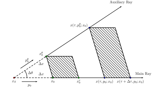
Fig. 2: The relation of the origin (shooting point) of the ray $x_{S}$ to its initial point $x_{0}$ in the proximal ray method for the determinant of the Jacobian.

The amplitude (11) requires the evaluation of the Jacobian (17) at the ray initial point $x_{0}$, at which the determinant is singular. We circumvent the problem analogously as in the ODE method by shifting the origin of the ray to a nearby point $x_{S}=x_{0}-\Delta x\cdot p_{0}/\|p_{0}\|$ (see figure 2), which yields $x_{S}=x(-\Delta\tau,p_{0};x_{0}),\,x_{0}^{\tau}=x(\Delta\tau,p_{0};x_{0})\,$ and $\,x_{0}^{\theta}=x(\Delta\tau,p_{0}^{\theta};x_{S})$ and the non-singular approximation to the determinant

$$q_{\tau}(0;x_{S})\approx\begin{vmatrix}\cfrac{x_{0}^{\theta}-x_{0}}{\Delta\theta}&\cfrac{x_{0}^{\tau}-x_{0}}{\Delta\tau}\end{vmatrix}.$$

Finally, the point $x_{0}^{\theta}$ corresponds to a rotation of $x_{0}$ by an angle $\Delta\theta$ around the origin of the ray $x_{S}$,

$$x_{0}^{\theta}=x_{S}+\Delta x\dfrac{p_{0}^{\theta}}{\|p_{0}^{\theta}\|},\quad p_{0}^{\theta}=\begin{pmatrix}\cos\Delta\theta&-\sin\Delta\theta\\ \sin\Delta\theta&\cos\Delta\theta\end{pmatrix}p_{0}.$$

We observe that $q$ (and hence the amplitude $A$) depends on the choice of the ray origin $x_{S}$, which is determined by the increment $\Delta x$. In a homogeneous 2D medium, the amplitude decays as $A(x)\sim\sqrt{\Delta x}/\sqrt{\Delta x+\|x\|}$. Assuming $\Delta x\ll\|x\|$, the amplitude behaves as $A(x)\approx\sqrt{\Delta x}/\sqrt{\|x\|}$ indicating that the shift by $\Delta x$ essentially corresponds to a scaling factor.

2.4 Reversing rays

The computation of the ray trajectories is at the core of our Hamilton-Green (HG) solver. For the solver to handle both the forward and the adjoint problems, it has to be capable of propagating the pressure wave both from the domain towards the sensors and from the sensors back into the domain. A naive approach would entail treating these two problems separately i.e. computing the ray trajectories for each independently. However, here the natural choice is to shoot the rays from the sensors into the domain. In the following we show that such trajectories are reversible. Hence, they can be used to propagate the wave in both directions. We derive an expression for the reversed phase $\phi_{R}$ and the reversed amplitude $A_{R}$ over the reversed ray $x_{R}(t)$ in terms of the original phase $\phi$ and amplitude $A$ over the original ray $x(t)$.

2.4.1 Reversed trajectory and phase

Given a ray $x(t)$ shot from $x(0)=x_{A},\,p(0)=p_{A}$ to $x(T)=x_{B},p(T)=p_{B}$, we obtain its reversed ray as

$$x_{R}(t)=x(T-t),\qquad p_{R}(t)=-p(T-t).$$

Following the principle of reciprocity, we observe that the reversed ray also satisfies the Hamiltonian system with the initial conditions $x_{R}(0)=x_{B},p_{R}(0)=-p_{B}$. Summarising, for $x$ and $x_{R}$ it holds

$$x_{R}(0)=x(T)=x_{B}, x_{R}(T)=x(0)=x_{A},$$

$$p_{R}(0)=-p(T)=-p_{B}, p_{R}(T)=-p(0)=-p_{A}.$$

Recalling that the phase is essentially the propagation time (c.f. change of variables $t^{\prime}=T-t$), we immediately obtain

$$\phi_{R}(t)=\phi(x(T-t))=T-t+\phi(x_{0}).$$ (18)

2.4.2 Reversed amplitude

In the same spirit we would like to express the reversed amplitude $A_{R}(x_{R}(t))$ along the reversed ray $x_{R}(t)$ in terms of the original trajectory $x$, phase $\phi$ and the inverse ray density (Jacobian determinant) $q$. From the first principle the reversed inverse ray density, $q_{R}$, is the determinant of the Jacobian of $x_{R}$ w.r.t. the initial point of $x_{R}$ (which is the end point of $x$) i.e. $x_{T}:=x(T;x_{0})=x_{R}(0;x_{T})$

$$q_{R}(t;x_{T})=\left|D_{x_{T}}x_{R}(t;x_{T})\right|,$$ (19)

with

$$x_{R}(t;x_{T}):=x(T-t;x_{0})$$ (20)

Substituting (20) into (19), applying the chain rule and the determinant calculus yields

$$q_{R}(t;x_{T})=|D_{x_{T}}x(T-t;x_{0})|=|D_{x_{0}}x(T-t;x_{0})|\left|\frac{\partial x_{0}}{\partial x_{T}}\right|,$$

where $|D_{x_{0}}x(T-t;x_{0})|=q(T-t;x_{0})$ by definition and

$$|\partial x_{0}/\partial x_{T}|=|\left.\partial x(t;x_{0})/\partial x_{0}\right|_{t=T}|^{-1}=|\left.D_{x_{0}}x(t;x_{0})\right|_{t=T}|^{-1}=1/q(T;x_{0}).$$

Thus we expressed $q_{R}$ in terms of $q$

$$q_{R}(t;x_{T})=\frac{q(T-t;x_{0})}{q(T;x_{0})}.$$ (21)

The reversed amplitude $A_{R}(x_{R}(t;x_{T}))$ along the reversed ray $x_{R}(t)$ in terms of reversed quantities follows immediately from (11)

$$A_{R}(x_{R}(t;x_{T}))=A_{0}(x_{T})\sqrt{\frac{q_{R}(0;x_{T})}{q_{R}(t;x_{T})}}\frac{\eta(x_{T})}{\eta(x_{R}(t;x_{T}))}.$$ (22)

Substituting the reversed quantities with (20) and (21) we obtain an expression in terms of the original quantities $x$ and $q$

$$A_{R}(x_{R}(t;x_{T}))=A_{0}(x_{T})\sqrt{\frac{q(T;x_{0})}{q(T-t;x_{0})}}\frac{\eta(x_{T})}{\eta(x(T-t;x_{0}))}.$$

2.5 Caustics and shadow regions

We finish this section with the discussion of the two limitations of the ray tracing approach, the caustics and the shadow regions.

Caustics

A caustic is a set of points at which the determinant of the Jacobian of the coordinate change, (12), becomes singular.

As the determinant of the Jacobian (12) is in the denominator of the amplitude formula (11), the latter becomes unbounded at caustics. Thus (11) cannot be used to compute the amplitude directly at and beyond the caustic. The following modification has been proposed beyond the caustic (but not at the caustic itself)

$$A(x(t,x_{0}))=A(x_{0})\frac{\eta(x_{0})}{\eta(x(t;x_{0}))}\sqrt{\left|\frac{q(0;x_{0})}{q(t;x_{0})}\right|}e^{-im(t)\frac{\pi}{2}},$$ (23)

where $m(t)$ is the Keller-Maslov index which counts the number of times the ray crosses a caustic (see e.g. [63]). To control the numerical integration error of the amplitude in the neighborhood of the caustic point, we set the ray amplitudes $A(x(t,x_{0}))$ to 0 for all times for which $|q(t;x_{0})|<\epsilon$ with a small parameter $\epsilon=q(0;x_{0})$. Once the determinant magnitude becomes large enough $|q(t;x_{0})|\geq\epsilon$, we compute the amplitudes $A(x(t,x_{0}))$ behind the caustic according to (23) neglecting the complex factor $\exp(-im(t)\pi/2)$ which is essentially a phase shift experienced by the rays that cross the caustic. Taking the absolute value of $q(t;x_{0})$ in (23) annihilates the reversing of the associated ray tube coordinate system due to the caustic. A solution which holds at and beyond the caustic could be obtained e.g. using dynamic ray tracing or Gaussian beams, which are out of scope of this manuscript but will be explored in future work.

Shadow regions

In geometrical optics a shadow region is defined with respect to a point (here we choose $x_{0}\not\in\Omega$). A shadow region is a subset of the domain $\Omega_{x_{0}}^{S}\subset\Omega$ which cannot be reached along any ray trajectory originating from $x_{0}$, in other words we cannot “illuminate” it with rays shot from $x_{0}$. Consequently, any pressure propagating from a shadow region will not affect the pressure at the sensor located at $x_{0}$ when using the Hamilton-Green solver.

Therefore, in the sequel we assume that the sound speed $c(x)$ in $\Omega$ is non-trapping [38], that is for any phase space point $(x_{0},p_{0})$ there exists a finite time $T$ such that the ray $x(t,x_{0})$ with shooting angle $p_{0}$, satisfies $x(t,x_{0})\notin\Omega\,\;\forall T>t$. Due to relatively small variation of the sound speed in soft tissue, with a high probability a domain in a typical PAT experiment will be non-trapping. However, in the numerical simulations the issue can become more subtle. Even in absence of a shadow region there can be a region with only few rays. Such low penetration region can in turn become an effective numerical shadow region, when we cannot illuminate it with rays given a fixed numerical precision. In such case, adaptive techniques should be deployed to ensure that all the domain is covered with rays sufficiently densely. Such methods could employ inserting new rays into the cone if divergence is observed. For inspirational ideas we refer to the literature on wavefront tracking methods [64, 65, 74]. It is not immediately clear how adaptive methods can be implemented maintaining the efficiency of the one shot methods discussed here and a detailed study will be subject of future research.

3 Hamilton-Green solver for the forward and adjoint problems

In this section we derive the Hamilton-Green solver for the forward and adjoint problems in PAT. Our approach can be viewed as approximating the time derivative of the unknown heterogeneous Green’s function in the Green’s integral solution of the respective forward/adjoint wave equation along the rays via the ray equations. We note that the PAT sensors provide the natural shooting points for the rays. As shown in section 2.4 the same trajectories can be used in both the forward and the adjoint problem. In particular, in the proposed Hamilton-Green solver, the adjoint problem solution follows the ray trajectories while the forward formula uses the reversed ray trajectories.

We see the following benefits of our formulation against direct approximation of the pressure along rays: i) the resulting integral formulations highlight the parallels to the forward and adjoint/inverse transforms in ray based tomography e.g. X-ray CT, ii) the Green integral in ray coordinates is a convenient and natural formulation for PAT where we integrate along isotemporal surfaces, iii) our formulation allows to seamlessly plug in any numerical approximation to the homogeneous Green’s function $G_{0}$ which makes the ray approach more directly comparable to the numerical method used to obtain that approximation to $G_{0}$ and makes explicit the point source normalisation used, iv) the asymptotic error $\mathcal{O}(1/\omega)$ is confined to the approximation of the time derivative of the Green’s function $\tilde{G}^{\prime}:=\partial G/\partial t$, $\tilde{G}^{\prime}=G^{\prime}+\mathcal{O}(1/\omega)$ which leads to a higher order asymptotic error for the solution of both the forward and adjoint problems than when these solutions are directly approximated using ray equations.

3.1 Green’s solution to the wave equation

The general form of the fundamental solution of the wave equation for bounded and unbounded domains can be found e.g. in [6]. Here we restrict the presentation to the initial value and the source problem for the unbounded domain which are relevant to PAT, see section 1.

The Green’s solution to the initial value problem for the inhomogeneous wave equation with the density source term $\rho$

$$\square^{2}u =\rho(t,x),$$ (24a)

$$u(0,x) =\psi(x),$$ (24b)

$$u_{t}(0,x) =\psi_{0}(x),$$ (24c)

can be written as

$$u(t,x)=f(t,x)+h_{1}(t,x)+h_{2}(t,x)$$ (25)

with

$$f(t,x) =\int_{0}^{t^{+}}\int_{\operatorname{\mathbb{R}}^{d}}G(t,x\mid t^{\prime},x^{\prime})\rho(t^{\prime},x^{\prime})\,\textrm{d}x^{\prime}\,\textrm{d}t^{\prime},$$ (26a)

$$h_{1}(t,x) =\int_{\operatorname{\mathbb{R}}^{d}}\frac{1}{c^{2}(x^{\prime})}G(t,x\mid 0,x^{\prime}){\color[rgb]{0,0. 0}\psi_{0}(x^{\prime}})\,\textrm{d}x^{\prime},$$ (26b)

$$h_{2}(t,x) =\int_{\operatorname{\mathbb{R}}^{d}}\frac{1}{c^{2}(x^{\prime})}\frac{\partial G}{\partial t}(t,x\mid 0,x^{\prime}){\color[rgb]{0,0. 0}\psi(x^{\prime})}\,\textrm{d}x^{\prime}.$$ (26c)

Here $G$ is the corresponding free space Green’s function in $\mathbb{R}^{d}$ and $f$ and $h=h_{1}+h_{2}$ independently solve

• : $\square^{2}f=\rho(t,x),\quad f(0,x)=0,\;f_{t}(0,x)=0,$

• : $\square^{2}h=0,\quad h(0,x)=\psi(x),\;h_{t}(0,x)=\psi_{0}(x).$

In acoustically homogeneous medium the free space Green’s functions can be calculated analytically

$$\operatorname{\mathbb{R}}^{2}:\quad G_{0}^{2}(t,x\mid t^{\prime},x^{\prime})=\frac{c}{2\pi}\frac{H(c(t-t^{\prime})-\|x-x^{\prime}\|)}{\sqrt{c^{2}(t-t^{\prime})^{2}-\|x-x^{\prime}\|^{2}}},\qquad$$ (27)

where $H(t)$ is the Heaviside step function

$$H(t)=\left\{\begin{array}[]{ll}0&t<0,\\ 1&t\geq 0,\end{array}\right.$$

and

$$\operatorname{\mathbb{R}}^{3}:\quad G_{0}^{3}(t,x\mid t^{\prime},x^{\prime})=\frac{\delta(c(t-t^{\prime})-\|x-x^{\prime}\|)}{4\pi\|x-x^{\prime}\|},$$ (28)

where $\delta(t)$ denotes the Dirac delta distribution with the usual weak definition

$$\int_{-\infty}^{\infty}\delta(t)\zeta(t)dt=\zeta(0)$$ (29)

holds for any Schwarz test function $\zeta$, see e.g. [6].

In subsections 3.3, 3.4 we will make use of the following invariances of (in general heterogeneous) free space Green’s functions

$$G(t,x\,|\,t^{\prime},x^{\prime}) =G(-t^{\prime},x^{\prime}\,|\,-t,x)\quad\quad\mbox{(time reversal)}$$ (30a)

$$G(t,x\,|\,t^{\prime},x^{\prime}) =G(t+T,x\,|\,t^{\prime}+T,x^{\prime}),\quad T>0\quad\quad\mbox{(time shift)}.$$ (30b)

3.2 Strong approximation to the Green’s function

In order to implement the Green’s formula within the ray tracing algorithm we need a strong approximation of the Green’s function and its derivative. For strict comparability, in the numerical experiments in section 5 we are using the Green’s function obtained numerically using k-Wave [70]. We note that such obtained Green’s function is not strictly shift invariant which will contribute to the discrepancies between the results obtained with k-Wave and the proposed Hamilton-Green solver.

3.3 Forward problem

We recall the PAT forward problem introduced in (1)

$$\square^{2}u =0, (t,x)\in(0,\infty)\times\mathbb{R}^{d},$$ (1a)

$$u_{t}(0,x) =0, x\in\mathbb{R}^{d},$$ (1b)

$$u(0,x) =u_{0}(x), x\in\mathbb{R}^{d},$$ (1c)

which is an initial value problem for the wave equation with heterogeneous sound speed $c\in\mathcal{C}^{\infty}(\operatorname{\mathbb{R}}^{d})$.

In the Hamilton-Green forward solver the time dependent pressure is obtained at each of the sensors separately using the cone of rays originating from this particular sensor. Using Green’s formula (26c) the pressure $u(t,x_{0})$ at a given time $t$ at a sensor location point $x_{0}$ can be written as

$$u(t,x_{0})=\int_{\mathbb{R}^{d}}\frac{1}{c^{2}(x^{\prime})}\frac{\partial}{\partial t}G(t,x_{0}\mid 0,x^{\prime})u_{0}(x^{\prime})\textrm{d}x^{\prime},$$ (32)

where $G(t,x\mid t^{\prime},x^{\prime})$ is an, in general, heterogeneous free-space Green’s function. Furthermore, for any $u_{0}$ compactly supported on $\Omega$ the integration can be restricted to the domain $\Omega$. Let $(\ell,\theta)\in\operatorname{\mathbb{R}}_{0+}\times\mathcal{S}^{d-1}$ be ray based coordinates for the rays originating from $x_{0}\not\in\Omega$. Assuming that these rays do not intersect in $\Omega$, they form a coordinate system in $\Omega$ and we can perform a formal change of coordinates in (32). However, the ray based coordinates parametrisation yields a useful approximation to (32) even if the rays intersect. In this parametrisation (32) becomes

$$u(t,x_{0})=\int_{0}^{T}\int_{\mathcal{S}^{d-1}}\frac{1}{c^{2}(x(\ell,\theta;x_{0}))}\frac{\partial}{\partial t}G(t,x_{0}\mid 0,x(\ell,\theta;x_{0}))\,u_{0}(x(\ell,\theta;x_{0}))\left|\frac{\textrm{d}x^{\prime}}{\textrm{d}(\ell,\theta)}\right|\,\textrm{d}(\ell,\theta).$$ (33)

The acquisition time $T\in\operatorname{\mathbb{R}}_{+}$ is chosen sufficiently large so that all the rays in the cone have left the domain i.e. $x(\ell,\theta;x_{0})\notin\Omega\,\,\forall\ell>T,\theta\in\mathcal{S}^{d-1}$. Furthermore, by the definition, the determinant of the Jacobian of the change of coordinates

$$\left|\frac{\textrm{d}x}{\textrm{d}(\ell,\theta)}\right|_{x(0)=x_{0}}=q(\ell,\theta;x_{0}).$$ (34)

Using the combined time reversal and shift invariances of Green’s functions (30) we can rewrite the Green’s function with the source at the sensor

$$G(t,x_{0}\,|\,0,x(\ell,\theta;x_{0}))=G(t,x(\ell,\theta;x_{0})\,|\,0,x_{0}).$$ (35)

Substituting (34) and (35) into (33) we obtain

$$u(t,x_{0})=\int_{0}^{T}\int_{\mathcal{S}^{d-1}} \frac{1}{c^{2}(x(\ell,\theta;x_{0}))}\frac{\partial}{\partial t}G(t,x(\ell,\theta;x_{0})\,|\,0,x_{0})\,u_{0}(x(\ell,\theta;x_{0}))\,q(\ell,\theta;x_{0})\,\textrm{d}(\ell,\theta).$$ (36)

As the Green’s function for heterogeneous domain $G$ is generally unknown, we propose the following approximation in (36). Assuming a constant sound speed in a small neighborhood $\mathcal{N}(x_{0})$ of $x_{0}$, we can locally approximate the heterogeneous Green’s function $G(t,x\,|\,0,x_{0})$ with the homogeneous Green’s function $G_{0}(t,x\,|\,0,x_{0})$ with sound speed $c_{0}$ equal to sound speed at the emission point $x_{0}$ i.e. $c_{0}=c(x_{0})$,

$$G(t,x\,|\,0,x_{0})\approx G_{0}(t,x\,|\,0,x_{0}),\quad x\in\mathcal{N}(x_{0}).$$

Equation (36) however, requires $G$ everywhere and the homogeneous function approximation is not valid outside of $\mathcal{N}(x_{0})$. To simplify notation we short hand the attenuation along the ray from $x_{0}$ to $x(\ell,\theta;x_{0})$ in the amplitude formula (11) as

$$\mu(\ell,\theta;x_{0})=\frac{\eta(x_{0})}{\eta(x(\ell,\theta;x_{0}))}\sqrt{\frac{q(0,\theta;x_{0})}{q(\ell,\theta;x_{0})}}.$$ (37)

Now, the ray based coordinate system allows us to extend the approximation propagating the homogeneous free space Green’s function $G_{0}(t,x_{0}\,|\,0,x_{0})$ along the ray $(x_{0},\theta)$ from $x_{0}$ to $x(\ell,\theta;x_{0})$ and compute the corresponding amplitude according to (11)

$$G(t,x(\ell,\theta;x_{0})\mid 0,x_{0})\approx G_{0}(t-\ell,x_{0}\mid 0,x_{0})\,\mu(\ell,\theta;x_{0}).$$ (38)

Assuming the time parametrization along the ray, $\ell$ is the time of propagation from $x_{0}$ to $x(\ell,\theta;x_{0})$ which directly corresponds to the phase (9). The latter effects a time shift in the Green’s function due to its explicit dependence on time (note that throughout our derivation the time dependence has been implicit through the parametrization of the trajectory).

We note that the choice of the approximation point to be the evaluation point, here the sensor $x_{0}$, is not coincidental but necessary for the appropriate speed of sound $c_{0}$ and hence time scaling of the homogeneous Green’s function $G_{0}$. This indeed was the reason for reversing the Green’s function in (35). Substituting (38) and (37) into (36) and rearranging the integration to reflect functional dependencies we arrive at

$$u(t,x_{0})=\eta(x_{0})\int^{T}_{0}\frac{\partial}{\partial t}G_{0}(t-\ell,x_{0}\mid 0,x_{0})\int_{\mathcal{S}^{d-1}}\eta(x(\ell,\theta;x_{0}))\sqrt{q(0,\theta;x_{0})q(\ell,\theta;x_{0})}\,u_{0}(x(\ell,\theta;x_{0}))\,\textrm{d}\theta\,\textrm{d}\ell.$$ (39)

Below we summarize the steps necessary to numerically evaluate (39) which corresponds to solving the forward problem (1) for a sensor located at $x_{0}$.

• Trace ray trajectories from $x_{0}$ such that they cover the domain $\Omega$ sufficiently densely (figure 3).

• Interpolate $u_{0}$ and $\eta$ at equitemporal points along the ray trajectories ($q$ is already available at these points), see A.1.

• Numerically evaluate the spherical integral along the isotemporal surfaces, $\ell=\mbox{const}$. Using mid-point rule this corresponds to summing the appropriately weighted contributions from all rays from $x_{0}$ at $\ell$.

• Convolve the result with the time derivative of the homogeneous Green’s function at $x_{0}$, $\frac{\partial}{\partial t}G_{0}(t,x_{0}\mid 0,x_{0})$.

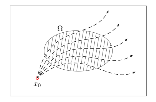
Fig. 3: Cone of rays from $x_{0}$ covering the domain $\Omega$ where the initial pressure $u_{0}$ is compactly supported.

3.4 Adjoint problem

The adjoint problem in PAT (3) is a time varying source problem for the free space wave equation with homogeneous initial conditions. Due to the linearity of the wave equation (3), the solution is a superposition of the corresponding solutions for each individual point mass source located at the sensor $x_{0}^{m},\;m=1,\dots,M$. Similarly as for the forward problem, in the adjoint Hamilton-Green solver we solve the adjoint problem for each mass source separately using the ray cone originating from the sensor $x_{0}$

$$\square^{2}v =\frac{\partial}{\partial t}\Big{(}g(T-t,x)\,\omega(T-t)\Big{)}\delta(x-x_{0}), (t,x)\in(0,T) \times\operatorname{\mathbb{R}}^{d},$$ (3a’)

$$v_{t}(0,x) =0, x \in\operatorname{\mathbb{R}}^{d},$$ (3b’)

$$v(0,x) =0, x \in\operatorname{\mathbb{R}}^{d}.$$ (3c’)

Analogously as for the forward problem, we start from the corresponding Green’s representation to the solution of the source problem (26a) evaluated at $t=T$

$$v(T,x)=\int_{\operatorname{\mathbb{R}}^{d}}\int_{0}^{T}G(T,x\mid t^{\prime},x^{\prime})\,\frac{\partial}{\partial t^{\prime}}\Big{(}g(T-t^{\prime},x^{\prime})\,\omega(T-t^{\prime})\Big{)}\delta(x^{\prime}-x_{0})\,\textrm{d}t^{\prime}\textrm{d}x^{\prime}.$$ (41)

Upon the change to ray based coordinate system (41) becomes

$$v(T,x(\ell,\theta;x_{0}))=\int_{0}^{T}\int_{\mathcal{S}^{d-1}} \underbrace{\int_{0}^{T}G(T,x\mid t^{\prime},x(\ell^{\prime},\theta^{\prime};x_{0}))\,\frac{\partial}{\partial t^{\prime}}\Big{(}g(T-t^{\prime},x(\ell^{\prime},\theta^{\prime};x_{0}))\,\omega(T-t^{\prime})\Big{)}\textrm{d}t^{\prime}}_{(\star)}$$

$$\times\underbrace{\delta(\ell^{\prime}-0)\delta(\theta^{\prime}-\theta)}_{=\delta(x(\ell^{\prime},\theta^{\prime};x_{0})-x(0,\theta;x_{0}))}q(\ell^{\prime},\theta^{\prime};x_{0})\,\textrm{d}\theta^{\prime}\textrm{d}\ell^{\prime},$$ (42)

where we chose to represent $x_{0}=x(0,\theta;x_{0})$ using the ray through $x=x(\ell,\theta;x_{0})$. Integrating $(\star)$ by parts, using the time shift invariance of the Green’s function to set the emission time to 0 and the variable change $t=T-t^{\prime}$ yields

$$(\star)= -\int_{0}^{T}\frac{\partial}{\partial t^{\prime}}G(T,x\mid t^{\prime},x(\ell^{\prime},\theta^{\prime};x_{0}))\,g(T-t^{\prime},x(\ell^{\prime},\theta^{\prime};x_{0}))\,\omega(T-t^{\prime})\textrm{d}t^{\prime}$$

$$+G(T,x,\mid T,x(\ell^{\prime},\theta^{\prime};x_{0}))g(0,x(\ell^{\prime},\theta^{\prime};x_{0}))\underbrace{\omega(0)}_{=0}$$

$$-G(T,x,\mid 0,x(\ell^{\prime},\theta^{\prime};x_{0}))g(T,x(\ell^{\prime},\theta^{\prime};x_{0}))\underbrace{\omega(T)}_{=0}$$

$$= \int_{0}^{T}\frac{\partial}{\partial t}G(t,x\mid 0,x(\ell^{\prime},\theta^{\prime};x_{0}))\,g(t,x(\ell^{\prime},\theta^{\prime};x_{0}))\,\omega(t)\textrm{d}t.$$ (43)

Substituting (3.4) into (42) and using the distributional calculus to evaluate the ray cone integral against the $\delta(\ell^{\prime}-0)\delta(\theta^{\prime}-\theta)$, we obtain

$$v(T,x(\ell,\theta;x_{0}))=q(0,\theta;x_{0})\int_{0}^{T}\frac{\partial}{\partial t}G(t,x\mid 0,x_{0})\,g(t,x_{0})\,\omega(t)\textrm{d}t.$$ (44)

To approximate the unknown heterogeneous Green’s function we again make use of a ray based approximation setting

$$G(t,x\mid 0,x(\ell,\theta;x_{0}))\approx G_{0}(t,x\mid 0,x(\ell,\theta;x_{0})),\quad x\in\mathcal{N}(x(\ell,\theta;x_{0})),$$

and outside of $\mathcal{N}(x(\ell,\theta;x_{0}))$ (in particular at the sensor $x_{0}$)

$$G(t,x_{0}\mid 0,x(\ell,\theta;x_{0}))\approx G_{0}(t-\ell,x(\ell,\theta;x_{0})\mid 0,x(\ell,\theta;x_{0}))\,\mu_{R}(\ell,\theta;x_{0}),$$

where $\mu_{R}$ is the analogously defined reversed attenuation in (22) i.e. attenuation between $x(\ell,\theta;x_{0})$ and $x_{0}$ along the reversed ray

$$\mu_{R}(\ell,\theta;x_{0}) =\frac{\eta(x(\ell,\theta;x_{0}))}{\eta(x_{0})}\sqrt{\frac{q_{R}(0,\theta;x(\ell,\theta;x_{0}))}{q_{R}(\ell,\theta;x(\ell,\theta;x_{0}))}}$$

$$=\frac{\eta(x(\ell,\theta;x_{0}))}{\eta(x_{0})}\sqrt{\frac{q(\ell,\theta;x_{0})}{q(0,\theta;x_{0})}}\phantom{x(\ell,\theta;x_{0})}=\frac{1}{\mu(\ell,\theta;x_{0})}.$$ (45)

Using the combined time shift and reversal invariances of Green’s function we rephrase the Green’s function in (44) with a source at the evaluation point $x(\ell,\theta;x_{0})$

$$v(T,x(\ell,\theta;x_{0}))=q(0,\theta;x_{0})\int_{0}^{T}\frac{\partial}{\partial t}G(t,x_{0}\mid 0,x(\ell,\theta;x_{0}))\,g(t,x_{0})\,\omega(t)\textrm{d}t$$ (46)

which will guarantee the correct speed of sound $c_{0}=c(x(\ell,\theta;x_{0})))$ for the homogeneous Green’s function $G_{0}$. Substituting the ray approximation and $\mu_{R}$ from (3.4) we arrive at the Hamilton-Green approximation to the adjoint solution

$$v(T,x(\ell,\theta;x_{0}))\approx\frac{\eta(x(\ell,\theta;x_{0}))}{\eta(x_{0})}\sqrt{q(0,\theta;x_{0})q(\ell,\theta;x_{0})}\int_{0}^{T}\frac{\partial}{\partial t}G_{0}(t-\ell,x(\ell,\theta;x_{0})\mid 0,x(\ell,\theta;x_{0}))\,g(t,x_{0})\,\omega(t)\textrm{d}t.$$ (47)

Equation (47) is naturally defined in ray based coordinates and needs to be interpolated on the Cartesian grid as described in the A.2. Summing over all sensors we obtain the adjoint of the original equation (3)

$$v(T,x)\approx \sum_{m=1}^{M}v(T,x(\ell^{m},\theta^{m};x_{0}^{m})).$$ (48)

The steps necessary for numerical evaluation of (47) which corresponds to the adjoint problem with one sensor located at $x_{0}$ are summarized below. We note that steps 1,2 are the same as for the forward problem and will be executed only once in an efficient implementation.

• Trace ray trajectories from $x_{0}$ such that they cover the domain $\Omega$ sufficiently densely (figure 3).

• Interpolate $\eta$ at equitemporal points in the domain ($q$ is already available at these points).

• Numerically evaluate the time integral. Using mid-point rule this corresponds to summing the data time series weighted by a shifted derivative of the homogeneous Green’s function $G_{0}$ with a sound speed $c_{0}=c(x(\ell,\theta;x_{0}))$. The details of efficient evaluation of $G_{0}$ are given in the A.3.

4 Error analysis of the Hamilton-Green solver

In this section we identify and quantify various contributions to the error of the Hamilton-Green approximation to the solution of the forward and adjoint PAT problems.

Asymptotic error in approximation of $G^{\prime}:=\partial G/\partial t$

The HG solver uses the first term of the WKB expansion to approximate the time derivative of the unknown (heterogeneous) Green’s function $G$, $G^{\prime}:=\partial G/\partial t$, on the domain along the rays. This implies that the asymptotic error of the approximation of $G^{\prime}$ is $\tilde{G}^{\prime}=G^{\prime}+\mathcal{O}(1/\omega)$.

The solution $u$ of the forward problem (39) is a convolution of the derivative of the Green’s function $G^{\prime}$ with the initial pressure $u_{0}$. Using the approximate $\tilde{G}^{\prime}$ instead, results in an approximation $\tilde{u}$. Switching to Fourier domain, we have the following asymptotic for this approximate solution $\left(\tilde{u}\right)^{\wedge}=\left(\tilde{G}^{\prime}\right)^{\wedge}\left(u_{0}\right)^{\wedge}=\left(\left(G^{\prime}\right)^{\wedge}+\mathcal{O}(1/\omega)\right)\left(u_{0}\right)^{\wedge}=\left(G^{\prime}\right)^{\wedge}\left(u_{0}\right)^{\wedge}+\mathcal{O}(1/\omega)\left(u_{0}\right)^{\wedge}=\left(u\right)^{\wedge}+\mathcal{O}(1/\omega)\left(u_{0}\right)^{\wedge}$ as opposed to $\left(\breve{u}\right)^{\wedge}=\left(u\right)^{\wedge}+\mathcal{O}(1/\omega)$ when the solution is approximated directly by the ray equations. Making a conservative assumption that $u_{0}$ is compactly supported of bounded variation, implies the decay of its Fourier transform $|\left(u_{0}(\xi)\right)^{\wedge}|=\mathcal{O}(1/|\xi|)$ as $|\xi|\rightarrow\infty$ yielding a higher order asymptotic error for the HG solution $\tilde{u}=u+\mathcal{O}(\omega^{-1}|\xi|^{-1})=u+\mathcal{O}(\omega^{-2})$.

When we assume $u_{0}\in C_{0}^{\infty}(\mathbb{R}^{d})$ (as we do here), its Fourier transform decays faster than any polynomial $|\left(u_{0}(\xi)\right)^{\wedge}|=o(|\xi|^{-n}),\;\forall n\in\mathbb{N}$ as $|\xi|\rightarrow\infty$ and consequently so does the asymptotic error of the HG solution $\tilde{u}=u+o(\omega^{-n})$.

As the asymptotic error of $\tilde{G}^{\prime}$ enters the adjoint problem (47) in the same way i.e. the solution of (47) also contains the convolution of $G^{\prime}$ but this time with the PAT data $g$, the same argument holds for the asymptotic error of the solution to the adjoint problem with analogous smoothness assumptions on data $g$.

Accuracy of numerical integration of the ray trajectories

The solution to the Hamiltonian system (7) results in ray trajectories $x(t)$, which are an essential building block of our solver. These ray trajectories are computed using a second order Runge-Kutta method. Assuming that the exact sound speed is known, the error commited at each step is $\mathcal{O}(h^{3})$, where $h$ is the step size [5]. Therefore, the accumulated overall error for the whole trajectory is $\mathcal{O}(h^{2})$.

Grid interpolation error

Another source of error is the interpolation between Cartesian and ray grids. We use nearest-neighbour interpolation in both directions: from Cartesian to ray and from ray to Cartesian (see A). For a Cartesian grid with spacing $h$, the order of the error using nearest-neighbour interpolation is $\mathcal{O}(h)$. Conversely, the order of the error when converting from the ray grid to a Cartesian grid is $\mathcal{O}(h)$, where $h$ describes the maximum distance between neighbouring points along the trajectory or neighbouring points on the wavefront.

Accuracy of approximation of free space Green’s function $G_{0}$ and its time derivative $G_{0}^{\prime}$

The forward (39) and adjoint (47), (48) formulae require an approximation of the free space Green’s function $G_{0}$ or its time derivative $G_{0}^{\prime}$ . The free space Green’s function is a distribution with a singularity at the origin (cf. equations (27) and (28)) which we compute as an impulse response to a strong approximation to $\delta$. The so approximated $G_{0}$ is has no singularities and is finite (when e.g. using Gaussian strong approximation with small tail truncation). Alternatively, $G_{0}$ can be obtained solving the wave equation with a numerical method and an approximation of $\delta$ consistent with the method, see also A.3. As the $G_{0}$ approximation is obtained independently, we can tune it to be of the same or lower order as the interpolation errors. The approximation of the derivative $G_{0}^{\prime}$ follows analogously.

Error resulting from reflections, caustics and shadow regions

When a wave traverses an interface between two media, part of its energy is reflected back and part of its energy is transmitted. The strength of the reflection depends on the smoothness of the sound speed respective to the wave length. The Hamilton-Green solver does not account for the reflected part, since it only propagates the pressure at the wavefront. As discussed in Subsection 2.5 the presence of caustics also limits the accuracy of our solver, since the determinant becomes singular and amplitude blows up at caustics. To control this error, we set to 0 the amplitudes along the rays in the neighbourhood of a caustic region. As no rays pass through numerical shadow regions, no contribution to pressure is recorded from these regions. These regions however, naturally correspond to very low ray densities and their contribution should be minimal.

In B we study the effect of the caustics in an acoustic lens which however highly exaggerates the issue. We performed no dedicated studies bounding the error introduced by reflections and shadow regions. However, we know that caustics, reflections and shadow regions are absent in the homogeneous case thus there we have control over all other errors (ray trajectories, grid interpolation and Green’s function), our solver converges in the homogeneous case at the order determined by the lowest order of the numerical scheme. Finally, we expect the errors introduced by reflections, caustics and shadow regions to be small when the changes of sound speed in the domain are subtle, which is in general the case in soft tissue [44].

5 Evaluation of the Hamilton-Green solver

In this section we evaluate the accuracy of the Hamilton-Green solver (HG) for the forward and adjoint PAT problems. We first discuss the numerical convergence of the solver for homogeneous sound speeds and then move to heterogeneous sound speed phantom emulating vessels embedded in a soft tissue. The HG solutions are compared against the first order pseudospectral method implemented in k-Wave toolbox [70]. The acoustic solver in k-Wave was extensively validated and its performance compared against analytical solutions [71, 43], other numerical models [24, 62] and experimental measurements [61, 76]. Our examples are restricted to 2D for ease of visualisation. An efficient GPU implementation enabling handling large image volumes will be the subject of a sequel paper along with the integration of the solver with iterative methods which can take full benefit of its flexibility. Therefore, we defer the discussion of the computational efficiency to that later work.

5.1 Error Analysis of the Forward Problem

We consider a discretised rectangular domain $\Omega$ of dimensions 512$\times$1024 with grid spacing $\Delta x=25$ [$\mu$m] and homogeneous sound speed $c_{0}=1,500$ [m/s]. We compute the solutions for three smooth initial pressure conditions $u_{i}$, $i\in\{1,2,3\}$

$$u_{i}(x,y)=e^{-\frac{(x-x_{i})^{2}+(y-y_{i})^{2}}{\sigma^{2}}},$$ (49)

where $(x_{1},y_{1})=(6.35,10.25)$ [mm], $(x_{2},y_{2})=(6.35,15.35)$ [mm] and $(x_{3},y_{3})=(6.35,20.48)$ [mm] and $\sigma=400$ [$\mu$m]. The Gaussian serves as a smooth alternative to a ball allowing to bypass the use of the smoothing filter in k-Wave simulations and reduce the errors at the boundary. For compactness of visualisation, a superposition of these individual initial pressure conditions, $\sum_{i}u_{i}$, is shown in figure 4(a).

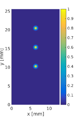
((a))

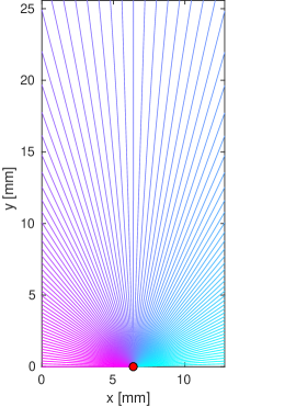
((b))

Fig. 4: Homogeneous sound speed. (a) Sum of initial pressure conditions $\sum u_{i}$. (b) Subset of ray trajectories from $x_{0}=(6.35,0)$ [mm].

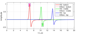
((a))

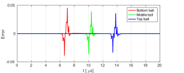
((b))

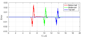
((c))

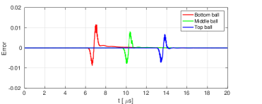
((d))

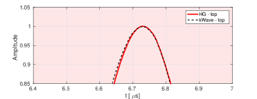
((e))

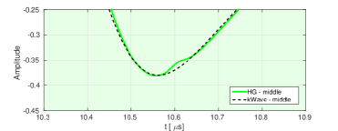
((f))

Fig. 5: Homogeneous sound speed. Comparison between HG and k-Wave forward solutions at $x_{0}$ for decreasing time step length $\Delta t\in\{8,4,2\}$ [ns].

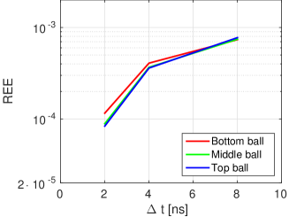
((a))

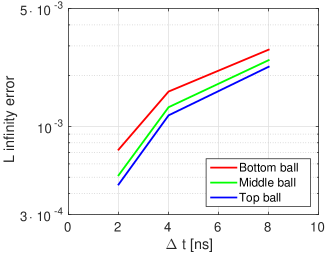
((b))

Fig. 6: Homogeneous sound speed. Convergence of the forward HG solver with decreasing time step $\Delta t\in\{8,4,2\}$ [ns] in terms of (a) REE and (b) $\ell_{\infty}$ error.

We place a single sensor at $x_{0}=(6.35,0)$ [mm] and shoot 4,000 rays in directions equisampling the angle range $[0,\pi]$. A subset of the trajectories obtained is shown in figure 4(b). These trajectories are straight lines, as expected in the homogeneous case. We denote with $g^{kW}_{i}=\mathcal{P}_{kW}(u_{i})$ and $g^{HG}_{i}=\mathcal{P}_{HG}(u_{i})$ the k-Wave and HG solutions of the forward problem for the initial pressure $u_{i}$. We evaluated both methods for time step lengths $\Delta t\in\{2,4,8\}$ [ns]. In figure 5(a) we plot the solutions at $x_{0}$ for each of the initial conditions individually. The HG solution (thick line) is superposed over k-Wave solution (thin line), the time step length is $\Delta t=8$ [ns]. We colour coded the initial conditions: bottom (the ball closest to the sensor) in red, middle in green and top in blue. Even for this coarse step, both solutions differ by at most 5% (see figure 5(b)). All pressure time series were normalised by $\ell_{\infty}$ norm of the k-Wave solution for the bottom ball, $\|g^{kW}_{1}\|_{\infty}=0.062$.

Figures 5(b-d) show the difference between the k-Wave and HG solutions for decreasing time steps $\Delta t\in\{8,4,2\}$ [ns]. We observe that halving the step essentially halves the $\ell_{\infty}$ error. This is in agreement with HG solver for homogeneous sound speed being exact up to the numerical errors due to interpolation between the grids, numerical integration and the approximation of the derivative of the Green’s function. Figure 6(a) shows the convergence of the relative energy error

$$REE^{\textnormal{forward}}(g^{HG})=\frac{\sum_{t_{i}\in(0,T)}(g^{kW}(t_{i})-g^{HG}(t_{i}))^{2}}{\sum_{t_{i}\in(0,T)}(g^{kW}(t_{i}))^{2}},$$ (50)

for each initial pressure with the decreasing time step length. The corresponding non-normalised $\ell_{\infty}$ errors,

$$\|g^{kW}-g^{HG}\|_{\infty},$$ (51)

are shown in figure 6(b). Both metrics behave similarly, thus henceforth we use REE with its convenient normalisation. The linear convergence is due to convergence of the grid interpolation error as the RK scheme is of higher order and the Green’s function derivative $G^{\prime}$ approximation is performed on a finer grid. Beyond time step length of $\Delta t$ = 2 [ns], the error due to spatial interpolation of $u_{i}$ with fixed grid spacing $\Delta x$ and accuracy of $G^{\prime}$ approximation become significant, and we cannot arbitrarily reduce the error solely by further time step refinement without also refining the spacial grid for $u_{0}$ and the $G^{\prime}$ approximation.

5.2 Error Analysis of the Adjoint Problem

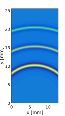
((a))

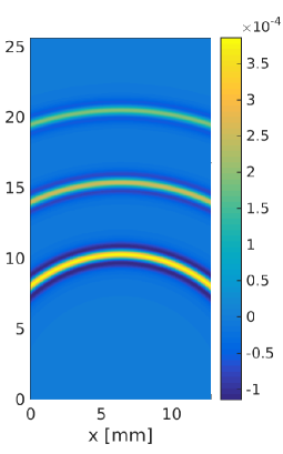
((b))

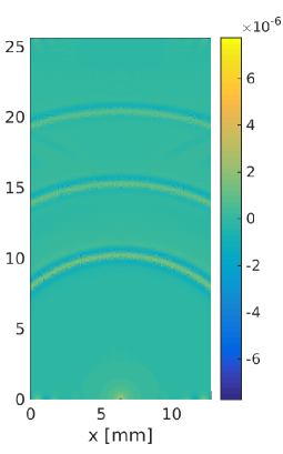
((c))

Fig. 7: Homogeneous sound speed. Time step $\Delta t=2$ [ns]. (a) Sum of adjoint k-Wave solutions $\sum_{j}\mathcal{P}_{kW}^{\star}(g^{kW}_{j})$. (b) Sum of adjoint HG solutions $\sum_{j}\mathcal{P}_{HG}^{\star}(g^{kW}_{j})$. (c) Difference between k-Wave and HG.

We solve the adjoint PAT problem for the simulated data $g^{kW}_{j},\;j\in\{1,2,3\}$ obtained with k-Wave in the previous section 5.1. The k-Wave solution is assumed to have no errors, which allows us to explore the error in our adjoint solver independently from the forward. Because of the reversibility of rays, we can reuse the ray trajectories obtained for the forward problem. In figure 7 we plot the sum of the three adjoint solutions for $g^{kW}_{j}$ obtained with k-Wave (a), HG (b) and their difference (c) for time step $\Delta t=2$ [ns]. The amplitude profile along the central cross-section $x=6.35$ [mm] is shown in Figure 8(a). Similarly, as for the forward problem, the $\ell_{\infty}$ error of the adjoint solution is in the order of 1%.

The convergence of the relative energy error for the adjoint problem for $g=g^{kW}_{j},\;j=\{1,2,3\}$

$$REE^{\textnormal{adjoint}}(g)=\frac{\sum_{x_{i}\in\Omega}((\mathcal{P}^{*}_{kW}\,g)(x_{i})-(\mathcal{P}^{*}_{HG}\,g)(x_{i}))^{2}}{\sum_{x_{i}\in\Omega}((\mathcal{P}^{*}_{kW}\,g)(x_{i}))^{2}}$$ (52)

with the decreasing time step is depicted in Figure 8(b) evidencing that HG adjoint solver is also exact for homogeneous sound speeds up to the same numerical errors as discussed for the forward problem.

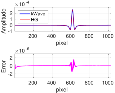
((a))

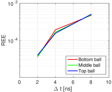
((b))

Fig. 8: Homogeneous sound speed. (a) Adjoint solution profile through $x=6.35$ [mm] for k-Wave and HG with $\Delta t=2$ [ns]. (b) Convergence of adjoint HG solver with decreasing time step $\Delta t=\{8,4,2\}$ [ns].

5.3 Simulated 2D Vessel Phantom with Heterogeneous Sound Speed

We complete our simulations with an experiment using a more realistic vessel phantom visualised in 9(a). The domain $\Omega$ was discretised with $128\times 256$ equispaced grid points with $\Delta x=100$ [$\mu$m]. The sound speed $c(x)$ shown in figure 9(c) was generated with the peaks() function in MATLAB and $c(x)\in 1,500\pm 10\%$ [m/s]. The time step was set to $\Delta t=10$ [ns] for both k-Wave and HG simulations. To avoid Gibbs phenomena in k-Wave, the initial pressure is a priori smoothed, see figure 9(b).

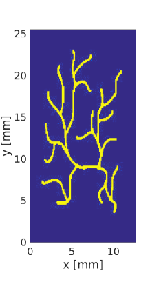
((a))

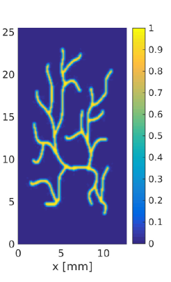
((b))

((c))

Fig. 9: (a) Initial pressure (without smoothing). (b) Initial pressure $u_{0}(x)$ (k-Wave smoothing). (c) Sound speed $c(x)$.

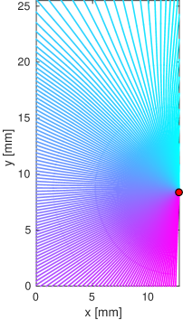
((a))

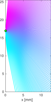
((b))

((c))

Fig. 10: Ray trajectories from 3 randomly chosen sensors.

Forward problem

We place a sensors at each grid point on the boundary of $\Omega$ amounting to 764 sensor in total. From each sensor location we shoot 4,000 rays with direction angles uniformly distributed between 0 and 2$\pi$ to ensure that we cover the entire domain. In figure 10 we exhibit a subset of trajectories for three sensors chosen at the random. Due to heterogeneity of $c$, these trajectories are no longer straight lines and present the two problematic scenarios: caustics (figure 10(c)) and shadow regions (figure 10(b-c)). We note that the pseudo-spectral finite difference method in k-Wave is a full wave solver and as such not affected neither by caustics nor shadow regions. In figure 11 we plot the sinograms for k-Wave, HG and their difference. The sinograms were normalised to 1 using the $\ell_{\infty}$ norm of the k-Wave solution, $\|g^{kW}\|_{\infty}=0.9329$. The $\ell_{\infty}$ error of the HG sinogram is significantly larger than in the homogeneous case (albeit $\ell_{\infty}$ appears a pessimistic metric in this case) while its REE is 1.99%.

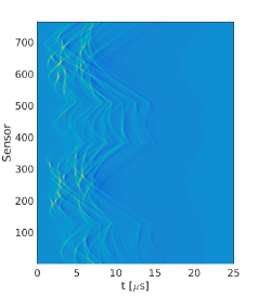
((a))

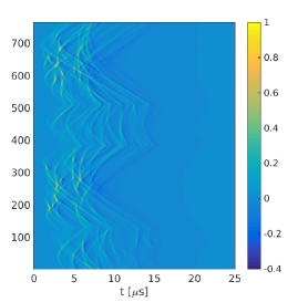
((b))

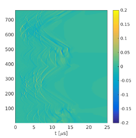
((c))

Fig. 11: (a) k-Wave sinogram. (b) HG sinogram. (c) Difference between k-Wave and HG sinograms.

Consistent forward-adjoint

We compute the k-Wave adjoint with the k-Wave forward data and the HG adjoint with its corresponding HG forward data. The results for these simulations are shown in figures 12(a-b). The overall structure of the adjoints is the same, containing similar artefacts for both methods. However, we observe more significant differences in the bottom left part of the image (c.f. figure 12(c)). The $\ell_{\infty}$ norm of the HG adjoint is on the order of 20%, although the large errors are concentrated in small region of the image. Here, the REE is equal to 2.23%.

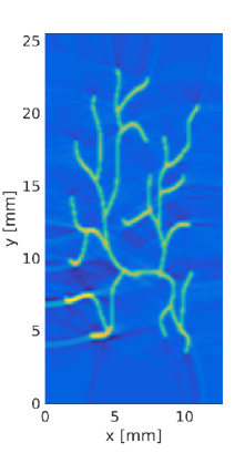
((a))

((b))

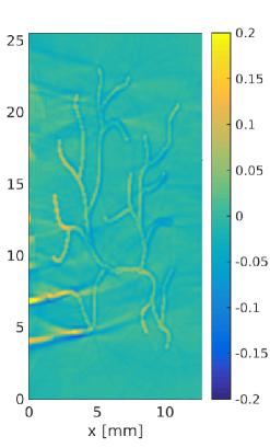
((c))

((d))

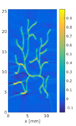
((e))

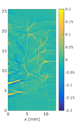
((f))

Fig. 12: (a) k-Wave adjoint (gold standard). (b) HG adjoint. (c) Difference between k-Wave and HG adjoints (same as error of HG adjoint). (d) k-Wave adjoint - HG data. (e) HG adjoint - k-Wave data. (f) Difference between mixed adjoints.

Mixed forward-adjoint

We solve two additional adjoint problems combining HG forward data with k-Wave adjoint solver and vice-versa to isolate forward/adjoint errors. Figure 12(d) shows the k-Wave solution of adjoint problem with HG forward data and figure 12(e) the HG adjoint with the k-Wave forward data. Both solutions have similar structure and artefacts also similar to the consistent case. The difference between the two mixed adjoints is shown in figure 12(f), with $\ell_{1}$ norm of around 20%. The REE for the combination HG forward data / k-Wave adjoint is 0.74% and for k-Wave forward data / HG adjoint is 1.79%, both lower than the REE for the consistent forward-adjoint, as one would expect.

6 Conclusions and outlook

In this paper we presented a novel acoustic Hamilton-Green solver for the forward and adjoint problems in PAT. The name is derived from the two main ingredients of the solver: the Hamiltonian system and the Green’s integral formula for the solution of the wave equation with initial data and time varying sources. The solver can be viewed as a ray tracing approximation of the heterogeneous Green’s function (more precisely its time derivative) in the Green’s integral formula evaluated on the ray induced grid. The main benefit of this approach is that the solution is computed for each sensor independently, opening to PAT the realm of ray based solvers which are well established for other tomographic modalities e.g. X-ray CT or PET. Furthermore, ray based solvers allow the flexibility to efficiently deal with sparse sensors and regions of interest thus potentially enabling online/real-time or dynamic reconstructions.

We analysed the error the proposed Hamilton-Green method, discussed its convergence in the homogeneous case and evaluated its accuracy in heterogeneous case on a 2D numerical vessel phantom against an established finite difference pseudo-spectral method implemented in k-Wave toolbox [70].

There are many open questions that need addressing to advance understanding and performance of the Hamilton-Green solver. A theoretical challenge is to find solution that holds valid in the presence of caustics without compromising the computational efficiency. In this context we are currently investigating two promising approaches: the dynamical ray tracing and Gaussian beams which both can be integrated with the Hamilton-Green solver. We are also working on an efficient implementation on GPU hardware which is imperative to apply the solver to large scale 3D real data problems. A particularly challenging implementation aspect is adaptive inserting and removing rays into and from the cone to control the impact of the changing ray density while maintaining the efficiency offered by one shot methods. Furthermore, we are working on coupling the Hamilton-Green solver with iterative methods for variational reconstruction which performance hinges on the ability to independently evaluate partial operators such as for instance the stochastic primal-dual hybrid gradient method recently proposed in [26].

Appendix A Implementation details

A.1 Interpolation: from Cartesian to ray based grid

When interpolating a function specified on Cartesian grid at a point in a ray based grid, $x(\ell,\theta;x_{0})$, we use the Cartesian grid point closest to $x(\ell,\theta;x_{0})$ in the $\ell_{2}$ sense.

Quantities in the code interpolated from Cartesian to ray based grid are: slowness $\eta$ and its gradient $\nabla\eta$, initial pressure $u_{0}$.

A.2 Interpolation: from ray based to Cartesian grid

When interpolating a function specified on ray based grid at a point in Cartesian grid, $x$, we use the the ray based grid point closest to $x$ in the $\ell_{2}$ sense.

Quantities in the code interpolated from ray based to Cartesian grid are: the solution of the adjoint problem (47), the reversed phase (propagation time), the reversed amplitude attenuation ($\mu_{R}$) used in the computation of the adjoint. To be precise, the latter can be obtained according to equations (18) and (3.4) from the (non-reversed) phase and amplitude attenuation (or ray density), respectively.

A.3 Approximating the homogeneous Green’s function at a point in the domain

Equation (47) requires knowledge of time derivative of the homogeneous Green’s function $G_{0}$ for a sound speed value $c_{0}=c(x(\ell,\theta;x_{0}))$. Obtaining $G_{0}$ for an exact value of $c_{0}=c(x(\ell,\theta;x_{0}))$ (in particular if $c$ was interpolated on the rays using an interpolation formula of an order higher than the nearest neighbour) would undue increase the computational cost. Instead, we precompute the Green’s function $G_{0}$ for a range of sound speeds $c_{\textrm{min}}\leq c(x)\leq c_{\textrm{max}},\forall x\in\Omega$ at equal increments, $\Delta c$ fine enough and use the tabulated $G_{0}$ with the closest sounds speed value to approximate $G_{0}$ with $c_{0}=c(x(\ell,\theta;x_{0}))$. The time derivative of $G_{0}$ is precomputed analogously.

Appendix B Effect of caustics on the HG forward solution in an acoustic lens

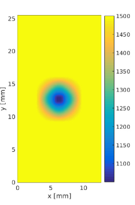
((a))

((b))

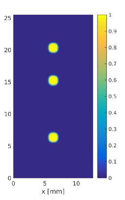
((c))

Fig. 13: (a) Acoustic lens sound speed $c(x)$. (b) Ray trajectories with a caustic in vicinity of $(6.35,15)$ [mm]. (c) Superposition of $\sum_{i}u_{i}$, each $u_{i}$ is an independent initial condition to the forward PAT problem.

To illustrate the effect of caustics we compute the forward propagation through an acoustic lens. We would like to stress, that the construction relies on a large variation of the speed of sound (here some 33%), hence such scenario is unrealistic to transpire in soft tissue where variations of sound speed are on the order of 5-10%.

Let $\Omega$ be a rectangular domain which we discretise with $N_{x}\times N_{y}=128\times 256$ equispaced grid points, $\Delta x$ = 100 [$\mu$m] with mostly homogeneous sound speed $c=1,500$ [m/s] which dips in the centre to $c_{\min}=1,050$ [m/s] forming an acoustic lens depicted in figure 13(a). This lens has the effect of focusing the rays.

We place a single sensor $x_{0}$ at the point $(6.35,0)$ [mm] on the boundary and compute the PAT data for this sensor for three initial pressures $u_{i}(x)$, $i\in\{b,m,t\}$, each $u_{i}(x)$, up to smoothing, assumes value 1 on a shifted ball of radius 8$\Delta x$. Figure 13(c), for compactness, shows their superposition $\sum_{i}u_{i}$.

To evaluate the impact of the caustic on HG solver, we compare the respective solutions at the sensor to the full wave solutions obtained with k-Wave. Both solvers use the same time step $\Delta t=10$ [ns].

HG solver shoots 4,000 rays from the sensor $x_{0}$ evenly sampling the angular range $[\pi/4,3\pi/4]$ to cover the relevant part of the domain. The ray cone is illustrated in figure 13(b). The inner trajectories focus in the vicinity of $(6.35,15)[mm]$. These rays form the caustic while the outer trajectories bend around that point and hence are unaffected by the caustic. The balls, $u_{i}$, were placed so to illustrate the differences in accuracy of the solution at the sensor in dependence of their location relative to the caustic: the bottom ball $u_{b}(x)$ is seen before any focusing, the middle ball $u_{m}(x)$ overlaps with the focus point and the top ball $u_{t}(x)$ is seen after a subset of rays passed the caustic.

The solutions at the sensor for each initial condition $u_{i}(x)$ computed with HG and k-Wave are plotted in 14(a), and their difference in 14(b). The results in 14(b) demonstrate that the solution for the initial pressure before the caustic is not affected (bottom ball, $u_{b}$). The error is largest for the initial pressure at the caustic (middle ball, $u_{b}$). This is mainly due to setting to 0 the ray amplitudes $A(x(t,x_{0}))$ for all times for which $|q(t;x_{0})|<\epsilon$ with a small parameter $\epsilon=q(0;x_{0})$ (note that the pulse shape is essentially preserved). The initial pressure behind the caustic is also affected but to a lesser degree (top ball, $u_{t}$). The amplitude contributions carried by the subset of rays that bends around the caustic are not affected at all, while the amplitude contribution of rays passing though the caustic undergo a phase shift (note the stretching of the pulse) according to (23). HG solution after the caustic does not account for the complex factor $\exp(-im(t)\pi/2)$ but it compensates for the caustic induced reversing of the associated ray tube coordinate system by taking the absolute value of $q(t;x_{0})$.

Figure 15(a) shows the trajectories of a small subset of rays in the transition region between the inner rays which form the caustic in $\Omega$ (light green) and the outer rays that bend around the caustic (dark blue). In the top of figure 15(b) we plot the corresponding determinants as functions of time $q(t;x_{0})$. $q(t;x_{0})$ are linear increasing until the rays reach the lens, for $t\approx 8$ [$\mu$s]. Thereafter, the determinants $q(t;x_{0})$ for different rays diverge, with $q(t;x_{0})$ for the three light green trajectories bending downwards and eventually becoming negative. As $q(t;x_{0})$ approach 0, the individual amplitudes blow up and become unbounded for $q(t;x_{0})=0$, as illustrated in the bottom of figure 15(b). Numerically, these amplitudes will be set to 0 for all $t:\;|q(t;x_{0})|<\epsilon$ thus this interval will not contribute to the solution at the sensor. Once $|q(t;x_{0})|\geq\epsilon$, these amplitudes will again contribute to the solution.

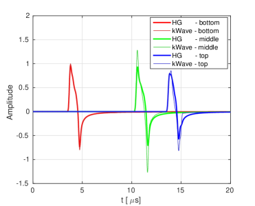
((a))

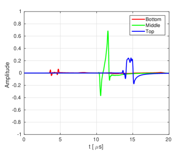
((b))

Fig. 14: (a) Forward solution $u(t,x_{0})$ at $x_{0}$ for initial conditions $u_{i},\;i\in\{b,m,t\}$ computed with HG and k-Wave. (b) Difference between HG and k-Wave solutions.

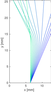
((a))

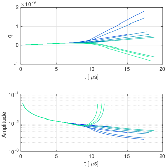
((b))

Fig. 15: (a) Subset of ray trajectories shot from $x_{0}$ illustrating the transition between the rays which form the caustic (light green) and those which bend around it (dark blue). (b) $q(t;x_{0})$ (top) and $A(x(t;x_{0}))$ (bottom) corresponding to the subset of ray trajectories in (a).

References

- [1] Rémi Abgrall and Jean-David Benamou. Big ray-tracing and eikonal solver on unstructured grids: Application to the computation of a multivalued traveltime field in the marmousi model. Geophysics, 64(1):230–239, 1999.
- [2] Mark Agranovsky and Peter Kuchment. Uniqueness of reconstruction and an inversion procedure for thermoacoustic and photoacoustic tomography with variable sound speed. Inverse Problems, 23(5):2089, 2007.
- [3] Simon Arridge, Paul Beard, Marta Betcke, Ben Cox, Nam Huynh, Felix Lucka, Olumide Ogunlade, and Edward Zhang. Accelerated high-resolution photoacoustic tomography via compressed sensing. Physics in Medicine and Biology, 61(24):8908, 2016.
- [4] Simon R Arridge, Marta M Betcke, Ben T Cox, Felix Lucka, and Brad E Treeby. On the adjoint operator in photoacoustic tomography. Inverse Problems, 32(11):115012, 2016.
- [5] Uri M Ascher and Linda R Petzold. Computer methods for ordinary differential equations and differential-algebraic equations, volume 61. Siam, 1998.
- [6] Gabriel Barton. Elements of Green’s functions and propagation: potentials, diffusion, and waves. Oxford University Press, 1989.
- [7] Amir Beck and Marc Teboulle. A fast iterative shrinkage-thresholding algorithm for linear inverse problems. SIAM journal on imaging sciences, 2(1):183–202, 2009.
- [8] Z. Belhachmi, T. Glatz, and O. Scherzer. A direct method for photoacoustic tomography with inhomogeneous sound speed. Inverse Probl., 32(4):045005, 2016.
- [9] G Beylkin. Imaging of discontinuities in the inverse scattering problem by inversion of a causal generalized radon transform. Journal of Mathematical Physics, 26(1):99–108, 1985.
- [10] Jean-David Benamou. Big ray tracing: Multivalued travel time field computation using viscosity solutions of the eikonal equation. Journal of Computational Physics, 128(2):463–474, 1996.
- [11] Jean-David Benamou and Ian Solliec. An eulerian method for capturing caustics. Journal of Computational Physics, 162(1):132–163, 2000.
- [12] Marta Betcke, Ben Cox, Nam Huynh, Edward Zhang, Paul Beard, and Simon R Arridge. Acoustic wave field reconstruction from compressed measurements with application in photoacoustic tomography. IEEE Transactions on Computational Imaging, 2017.
- [13] Max Born and Emil Wolf. Principles of optics: electromagnetic theory of propagation, interference and diffraction of light. Elsevier, 2013.
- [14] John Charles Butcher. Numerical methods for ordinary differential equations. John Wiley & Sons, 2016.
- [15] Shunhua Cao and Stewart Greenhalgh. Finite-difference solution of the eikonal equation using an efficient, first-arrival, wavefront tracking scheme. Geophysics, 59(4):632–643, 1994.
- [16] Vlastislav Červený, Mikhail M Popov, and Ivan Pšenčík. Computation of wave fields in inhomogeneous media—gaussian beam approach. Geophysical Journal International, 70(1):109–128, 1982.
- [17] V. Červený. Ray tracing algorithms in three-dimensional laterally varying layered structures, pages 99–133. Springer Netherlands, Dordrecht, 1987.
- [18] Vlastislav Červený. Seismic ray theory. Cambridge university press, 2005.
- [19] Antonin Chambolle and Thomas Pock. An introduction to continuous optimization for imaging. Acta Numerica, 25:161–319, 2016.
- [20] Antonin Chambolle, Matthias J. Ehrhardt, Peter Richtárik, and Carola-Bibiane Schönlieb. Stochastic Primal-Dual Hybrid Gradient Algorithm with Arbitrary Sampling and Imaging Applications. (ii):1–25, 2017.
- [21] Li-Tien Cheng, SJ Osher, and Jianliang Qian. Level set based eulerian methods for multivalued traveltimes in both isotropic and anisotropic media. In 73rd Annu. Int. Mtg., Soc. Expl. Geophys., Expanded abstracts, pages 1801–1804. Citeseer, 2002.
- [22] David Colton and Rainer Kress. Inverse acoustic and electromagnetic scattering theory, volume 93. Springer Science & Business Media, 2012.
- [23] BT Cox, JG Laufer, and PC Beard. The challenges for quantitative photoacoustic imaging. In Proc. SPIE, volume 7177, page 717713, 2009.
- [24] L Demi, BE Treeby, and MD Verweij. Comparison between two different full-wave methods for the computation of nonlinear ultrasound fields in inhomogeneous and attenuating tissue. In 2014 IEEE International Ultrasonics Symposium, pages 1464–1467. IEEE, 2014.
- [25] Nebojsa Duric, Peter Littrup, Alex Babkin, David Chambers, Stephen Azevedo, Arkady Kalinin, Roman Pevzner, Mikhail Tokarev, Earle Holsapple, Olsi Rama, and Robert Duncan. Development of ultrasound tomography for breast imaging: Technical assessment. Medical Physics, 32(5):1375–1386, 2005.
- [26] Matthias J Ehrhardt, Pawel Markiewicz, Antonin Chambolle, Peter Richtárik, Jonathan Schott, and Carola-Bibiane Schönlieb. Faster pet reconstruction with a stochastic primal-dual hybrid gradient method. In Wavelets and Sparsity XVII, volume 10394, page 103941O. International Society for Optics and Photonics, 2017.
- [27] Björn Engquist, Olof Runborg, and Anna-Karin Tornberg. High-frequency wave propagation by the segment projection method. Journal of Computational Physics, 178(2):373–390, 2002.
- [28] Björn Engquist and Olof Runborg. Computational high frequency wave propagation. Acta numerica, 12:181–266, 2003.
- [29] David Finch and Sarah K Patch. Determining a function from its mean values over a family of spheres. SIAM Journal on Mathematical Analysis, 35(5):1213–1240, 2004.
- [30] Sergey Fomel and James A Sethian. Fast-phase space computation of multiple arrivals. Proceedings of the National Academy of Sciences, 99(11):7329–7334, 2002.
- [31] P Gerstoft. Cabrillo 1.0: acoustic, elastic and poroelastic finite difference modelling, 2004.
- [32] Dan Givoli. Time Reversal as a Computational Tool in Acoustics and Elastodynamics. Journal of Computational Acoustics, 22(3):1430001, 2014.
- [33] Pierre A Gremaud and Christopher M Kuster. Computational study of fast methods for the eikonal equation. SIAM journal on scientific computing, 27(6):1803–1816, 2006.
- [34] Zijian Guo, Changhui Li, Liang Song, and Lihong V Wang. Compressed sensing in photoacoustic tomography in vivo. Journal of biomedical optics, 15(2):021311–021311, 2010.
- [35] Sverre Holm. Ultrasim-a toolbox for ultrasound field simulation. University of Oslo, 2001.
- [36] Nam Huynh, Edward Zhang, Marta Betcke, Simon Arridge, Paul Beard, and Ben Cox. A real-time ultrasonic field mapping system using a fabry–pérot single pixel camera for 3d photoacoustic imaging. In Proc. SPIE, volume 9323, pages 93231O–1, 2015.
- [37] Finn B Jensen, William A Kuperman, Michael B Porter, and Henrik Schmidt. Computational ocean acoustics. Springer Science & Business Media, 2000.
- [38] Peter Kuchment and Leonid Kunyansky. Mathematics of photoacoustic and thermoacoustic tomography. In Handbook of Mathematical Methods in Imaging, pages 817–865. Springer, 2011.
- [39] Cuiping Li, Nebojsa Duric, Peter Littrup, and Lianjie Huang. In vivo Breast Sound-Speed Imaging with Ultrasound Tomography. Ultrasound in Medicine and Biology, 35(10):1615–1628, 2009.
- [40] Hailiang Liu, Olof Runborg, and Nicolay Tanushev. Error estimates for gaussian beam superpositions. Mathematics of Computation, 82(282):919–952, 2013.
- [41] Yang Lou, Weimin Zhou, Thomas P Matthews, Catherine M Appleton, and Mark A Anastasio. Generation of anatomically realistic numerical phantoms for photoacoustic and ultrasonic breast imaging. Journal of biomedical optics, 22(4):041015, 2017.
- [42] Wangtao Lu, Jianliang Qian, and Robert Burridge. Babich’s expansion and the fast huygens sweeping method for the helmholtz wave equation at high frequencies. Journal of Computational Physics, 313:478–510, 2016.
- [43] Eleanor Martin, Yan To Ling, and Bradley E Treeby. Simulating focused ultrasound transducers using discrete sources on regular cartesian grids. IEEE transactions on ultrasonics, ferroelectrics, and frequency control, 63(10):1535–1542, 2016.
- [44] T Douglas Mast. Empirical relationships between acoustic parameters in human soft tissues. Acoustics Research Letters Online, 1(2):37–42, 2000.
- [45] Thomas P Matthews and Mark A Anastasio. Joint reconstruction of the initial pressure and speed of sound distributions from combined photoacoustic and ultrasound tomography measurements. Inverse problems, 33(12):124002, 2017.
- [46] Thomas P Matthews and Mark A Anastasio. Joint reconstruction of the sound speed and initial pressure distributions for ultrasound computed tomography and photoacoustic computed tomography. In Medical Imaging 2017: Ultrasonic Imaging and Tomography, volume 10139, page 101390B. International Society for Optics and Photonics, 2017.
- [47] Philip McCord Morse and K Uno Ingard. Theoretical acoustics. Princeton university press, 1968.
- [48] Linh V Nguyen. On singularities and instability of reconstruction in thermoacoustic tomography. Tomography and inverse transport theory, Contemporary Mathematics, 559:163–170, 2011.
- [49] Stanley Osher and James A Sethian. Fronts propagating with curvature-dependent speed: algorithms based on hamilton-jacobi formulations. Journal of computational physics, 79(1):12–49, 1988.
- [50] VWHK Pereyra, WHK Lee, and HB Keller. Solving two-point seismic-ray tracing problems in a heterogeneous medium part 1. a general adaptive finite difference method. Bulletin of the Seismological Society of America, 70(1):79–99, 1980.
- [51] V Pereyra. Ray tracing methods for inverse problems. Inverse Problems, 16(6):R1, 2000.
- [52] MM Popov, Ivan Pšenčík, and V Červenỳ. Computation of ray amplitudes in inhomogeneous media with curved interfaces. Studia Geophysica et Geodaetica, 22(3):248–258, 1978.
- [53] MM Popov and I Pšenčík. Ray amplitudes in inhomogeneous media with curved interfaces. Geofys. sb, 24:118–129, 1978.
- [54] Michael B Porter and Homer P Bucker. Gaussian beam tracing for computing ocean acoustic fields. The Journal of the Acoustical Society of America, 82(4):1349–1359, 1987.
- [55] Jianliang Qian and William W Symes. An adaptive finite-difference method for traveltimes and amplitudes. Geophysics, 67(1):167–176, 2002.
- [56] Jianliang Qian and Shingyu Leung. A local level set method for paraxial geometrical optics. SIAM Journal on Scientific Computing, 28(1):206–223, 2006.
- [57] Jianliang Qian, Plamen Stefanov, Gunther Uhlmann, and Hongkai Zhao. An efficient neumann series–based algorithm for thermoacoustic and photoacoustic tomography with variable sound speed. SIAM Journal on Imaging Sciences, 4(3):850–883, 2011.
- [58] James Ralston. Gaussian beams and the propagation of singularities. Studies in partial differential equations, 23:206–248, 1982.
- [59] Kui Ren, Hao Gao, and Hongkai Zhao. A hybrid reconstruction method for quantitative pat. SIAM Journal on Imaging Sciences, 6(1):32–55, 2013.
- [60] Paul G Richards and Keiiti Aki. Quantitative seismology: theory and methods. Freeman, 1980.
- [61] James Robertson, Eleanor Martin, Ben Cox, and Bradley E Treeby. Sensitivity of simulated transcranial ultrasound fields to acoustic medium property maps. Physics in Medicine and Biology, 62(7):2559–2580, mar 2017.
- [62] James LB Robertson, Ben T Cox, J Jaros, and Bradley E Treeby. Accurate simulation of transcranial ultrasound propagation for ultrasonic neuromodulation and stimulation. The Journal of the Acoustical Society of America, 141(3):1726–1738, 2017.
- [63] Olof Runborg. Mathematical models and numerical methods for high frequency waves. Commun. Comput. Phys, 2(5):827–880, 2007.
- [64] J. A. Sethian. A fast marching level set method for monotonically advancing fronts. Proceedings of the National Academy of Sciences, 93(4):1591–1595, 1996.
- [65] James A Sethian. Fast marching methods. SIAM review, 41(2):199–235, 1999.
- [66] J. A. Sethian. Fast Marching Methods and Level Set Methods for Propagating Interfaces. Computational Fluid Mechanics, 1998.
- [67] Wojciech Śmigaj, Timo Betcke, Simon Arridge, Joel Phillips, and Martin Schweiger. Solving boundary integral problems with bem++. ACM Transactions on Mathematical Software (TOMS), 41(2):6, 2015.
- [68] Plamen Stefanov and Gunther Uhlmann. Thermoacoustic tomography with variable sound speed. Inverse Problems, 25(7):075011, 2009.
- [69] Nicolay M Tanushev et al. Superpositions and higher order gaussian beams. Communications in Mathematical Sciences, 6(2):449–475, 2008.
- [70] Bradley E Treeby and Benjamin T Cox. k-wave: Matlab toolbox for the simulation and reconstruction of photoacoustic wave fields. Journal of biomedical optics, 15(2):021314–021314, 2010.
- [71] Bradley E Treeby, Jiri Jaros, Alistair P Rendell, and BT Cox. Modeling nonlinear ultrasound propagation in heterogeneous media with power law absorption using ak-space pseudospectral method. The Journal of the Acoustical Society of America, 131(6):4324–4336, 2012.
- [72] Junho Um and Clifford Thurber. A fast algorithm for two-point seismic ray tracing. Bulletin of the Seismological Society of America, 77(3):972–986, 1987.
- [73] Vlastislav Červenỳ and Ivan Pšenčík. Ray amplitudes of seismic body waves in laterally inhomogeneous media. Geophysical Journal International, 57(1):91–106, 1979.
- [74] Vetle Vinje. Traveltime and amplitude estimation using wavefront construction. Geophysics, 58(8):1157, 1993.
- [75] AL Virovlyansky. Ray travel times at long ranges in acoustic waveguides. The Journal of the Acoustical Society of America, 113(5):2523–2532, 2003.
- [76] Kejia Wang, Emily Teoh, Jiri Jaros, and Bradley E Treeby. Modelling nonlinear ultrasound propagation in absorbing media using the k-wave toolbox: experimental validation. In 2012 IEEE International Ultrasonics Symposium, pages 523–526. IEEE, 2012.
- [77] Yuan Xu and Lihong V Wang. Application of time reversal to thermoacoustic tomography. In Proceedings of SPIE, volume 5320, pages 257–263, 2004.
- [78] Minghua Xu and Lihong V Wang. Photoacoustic imaging in biomedicine. Review of scientific instruments, 77(4):041101, 2006.