Tilt estimator for 3D non-rigid pendulum based on a tri-axial accelerometer and gyrometer

Abstract

The paper presents a new observer for tilt estimation of a 3-D non-rigid pendulum. The system can be seen as a multibody robot attached to the environment with a ball joint for which there is no sensor. The estimation of tilt, i.e. roll and pitch angles, is mandatory for balance control for a humanoid robot and all tasks requiring verticality. Our method obtains tilt estimations using joints encoders and inertial measurements given by an IMU equipped with tri-axial accelerometer and gyrometer mounted in any body of the robot. The estimator takes profit from the kinematic coupling resulting from the pivot constraint and uses the entire signal of accelerometer including linear accelerations. Almost Global Asymptotic convergence of the estimation errors is proven together with local exponential stability. The performance of the proposed observer is illustrated by simulations.

I Introduction

One predominant goal of robotics is to be able to perform versatile interactions with the environment. In some cases, contact point constitute a link between the floating base of the robot and the environment, one example is legged locomotion, but also environment-related tasks such as torquing or drilling. Most of these tasks require the contact point to remain at a precise position and not to detach or slip. The observance of such a constraint generates a kinematic coupling allowing to model the robot as a kinematic chain attached to the environment with an unactuated joint. This can be simply summarized as a pendulum with the contact as the pivot point.

One main issue regarding this class of systems is that beside the unactuation, there is usually no direct measurement of the configuration of this pivot. Of course, properly estimating this configuration is of crucial importance in most tasks. Nevertheless, several kinds of sensors are sensitive to this configuration, and may be used to estimate it. The most broadly used ones are tri-axial accelerometer and gyrometer. This set of sensors provides invariant signals relative to different rotations around the gravitational field direction. This means that this orientation, usually called yaw angle, is not observable using this sensing system [1].

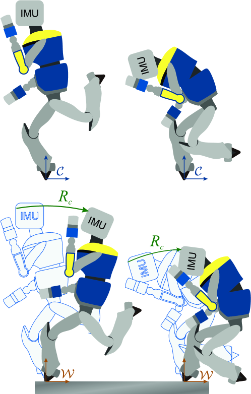
Figure 1: Top figures: the robot is attached to the environment through a 3D pivot joint. The encoders only provide the configuration in a local frame called control frame and represented by $\mathcal{C}$. Bottom figures: In the world frame $\mathcal{W}$ the configuration of the real robot is rotated compared to its value in the control frame (light wireframe robot). Only the IMU can provide data about this rotation, $R_{c}$. We need to account for encoders in this estimation, to distinguish local kinematics from pivot positions. For example the rotation $R_{c}$ is here identical in the right and the left lower figures with different IMU configurations.

Nevertheless, in robotics there is often a specific need for a precise estimation of the two other degrees of freedom, which can be referred to as roll and pitch angles, or simply tilt. These two degrees of freedom describe the configuration of the pivot relative to the gravitational field. They are then essential for maintaining balance for humanoid robots [15].

In this paper we provide a state estimator which aims at addressing this problem by providing a state estimator for the tilt of a pendulum which uses an accelerometer and a gyrometer, (i) without neglecting linear accelerations compared to gravity, (ii) well suited for articulated robot, and (iii) with a proven Lyapunov stability. Furthermore, this estimator reaches local exponential stability performances, which makes it particularly suitable for the use as a state feedback for closed-loop control. The idea behind this estimator is close to the recent development of Hua et al [5], who propose a tilt estimation when having a velocity measurement. The gyrometer and the kinematics constitute the velocity measurement in our case. But the estimator we develop is simpler and has better convergence properties in both theoretical and simulation points of view.

The section II presents the issue treated in this paper together with the model of the system and the sensors. The section III presents the development of the state estimator. The section IV analyzes the stability of the estimation error. Section V shows the performances of the estimator in simulation, and finally the section VI discusses the results and the properties of this estimator.

II Problem statement

The system is a robot linked to the environment through a ball joint called pivot. Without loss of generality we consider that the pivot is located at the origin of the inertial world frame ($\mathcal{W}$). The configuration of the pivot is a pure 3D rotation describing a transformation between the global frame and the local frame of the robot, also called control frame ($\mathcal{C}$). We represent this rotation by the rotation matrix $R_{c}\in\mathbb{R}^{3\times 3}$. For instance, the sensor $s$ located at position ${}^{c}p_{s}\in\mathbb{R}^{3}$ and orientation ${}^{c}R_{s}\in\mathbb{R}^{3\times 3}$ in $\mathcal{C}$ is actually at $p_{s}=R_{c}{}^{c}p_{s}$ and has the orientation $R_{s}=R_{c}{}^{c}R_{s}$ in $\mathcal{W}$. This problem is sketched in Figure 1.

There is no sensor providing the pivot configuration. Instead, the robot is equipped with an IMU consisting in an accelerometer and a gyrometer, both of them are on three axes. The position of this IMU may be not rigidly linked to the ball joint, and can be located in another body of the robot. Since the robot can modify its actuated joint kinematics the IMU may move in the control frame. Therefore, we have to consider its position $\,{}^{c}p_{s}\in\mathbb{R}^{3}$, its orientation represented by the orthogonal matrix $\,{}^{c}R_{s}\in\mathbb{R}^{3\times 3}$, together with their respective first-order time-derivatives $\,{}^{c}\dot{p}_{s}\in\mathbb{R}^{3}$ and $\,{}^{c}\omega_{s}\in\mathbb{R}^{3}$ such that $\,{}^{c}\dot{R}_{s}=S(^{c}\omega_{s})\,^{c}R_{s}$, where $S$ is the skew-symmetric operator.

The values of $\,{}^{c}\dot{p}_{s}$, $\,{}^{c}R_{s}^{T}$ , $\,{}^{c}\dot{p}_{s}$ and $\,{}^{c}\omega_{s}$ can be obtained through the positions and velocities of the joint encoders and are often the outcome of a motion controller. Therefore, these values are considered to be perfectly known.

The accelerometer provides the sum of the gravitational field and the linear acceleration of the sensor, expressed in the sensor frame. In other words we have

$$y_{a}=\,R_{s}^{T}\left(g_{0}e_{z}+\ddot{p}_{s}\right),$$ (1)

where $y_{a}$, $p_{s}$, $R_{s}$, $g_{0}$ and $e_{z}$ are respectively the accelerometer measurements, the position and the orientation of the IMU, standard gravity constant and a unit vector such that $-g_{0}e_{z}$ is the gravitational field.

The gyrometer provides the angular velocity of the IMU, expressed in the sensor frame. In other words

$$y_{g}=\,R_{s}^{T}\omega_{s},$$ (2)

where $\omega_{s}$ is the angular velocity vector of the sensor in the global frame such that $\dot{R}_{s}=S(\omega_{s})\,R_{s}$.

We can see from these equations that the measurements are invariant regarding rotations around the vector $e_{z}$ aligned with the gravitational field. Therefore, the orientation that can be estimated through this sensing system is incomplete. Nevertheless, we show here that one partial information is observable and consists in $R_{c}^{T}e_{z}$, the direction of the gravitational field in the local frame of the robot. This data is the most important variable required to control balance and may be considered as a measure of “verticality” in general.

By replacing $R_{s}$ and $p_{s}$ by $R_{c}{}^{c}R_{s}$ and $R_{c}{}^{c}p_{s}$ respectively and performing time-derivations and identification with (2) and (1) obtain

$$y_{g}= \,{}^{c}R_{s}^{T}\,{}^{c}\omega_{s}+\,^{c}R_{s}^{T}R_{c}^{T}\omega_{c},$$ (3)

$$y_{a}= \,{}^{c}R_{s}^{T}\left(\left(S(R_{c}^{T}\dot{\omega}_{c})+S^{2}(R_{c}^{T}\omega_{c})\right)\,^{c}p_{s}+2S(R_{c}^{T}\omega_{c})\,^{c}\dot{p}_{s}\right)$$

$$+\,^{c}R_{s}^{T}{}^{c}\ddot{p}_{s}+g_{0}\,^{c}R_{s}^{T}R_{c}^{T}e_{z}.$$ (4)

where $\omega_{c}$ is the angular velocity vector of the pendulum such that $\dot{R}_{c}=S(\omega_{c})\,R_{c}$.

In the following section we develop the state observer for the estimation of $R_{c}^{T}e_{z}$.

III State estimator

III-A State definition

The first variable we define is the pivot angular velocity expressed in the control frame $y_{1}=R_{c}^{T}\omega_{c}$. Replacing this in (3) we have

$$y_{1}= {}^{c}R_{s}\left(y_{g}-{}^{c}R_{s}^{T}\,{}^{c}\omega_{s}\right),$$ (5)

and since all the rightmost variables are known or measured we may consider $y_{1}$ as measured.

Let’s define also the following state variables:

$$x_{1} = S(^{c}p_{s})y_{1}-\,^{c}\dot{p}_{s},$$ (6)

$$x_{2} = R_{c}^{T}e_{z},$$ (7)

with $x_{1}\in\mathbb{R}^{3}$ and $x_{2}\in\mathbb{S}^{2}$, with the set $\mathbb{S}^{2}\subset\mathbb{R}^{3}$ is the unit sphere centered at the origin, and defined as

$$\mathbb{S}^{2}=\left\{x\in\mathbb{R}^{3}/\left\|x\right\|=1\right\}.$$

The variable $x_{2}$ is the state we aim at estimating and cannot be obtained algebraically. On the contrary, the variable $x_{1}$ is considered measured since we know ${}^{c}p_{s}$ , ${}^{c}\dot{p}_{s}$ and $y_{1}$, and is the opposite of the linear velocity of the IMU expressed in the local frame $x_{1}=-R_{c}^{T}\dot{p}_{s}$. In this study we use this data to build a tilt estimator able to distinguish gravity from accelerations, similarly to [5].

By left-multiplying Equation (4) by ${}^{c}R_{s}$ and replacing the expression of $y_{1}$ of equation (5) we get

$$S(^{c}p_{s})R_{c}^{T}\dot{\omega}_{c}+S(\,^{c}\dot{p}_{s})y_{1}-{}^{c}\ddot{p}_{s}=$$

$$\qquad\;\;\;-S(y_{1})\left(S(\,^{c}p_{s})y_{1}-\,^{c}\dot{p}_{s}\right)+g_{0}R_{c}^{T}e_{z}-{}^{c}R_{s}y_{a}.$$ (8)

We notice that the left member of equation (8) is the first order time-derivative of $x_{1}$. This, together with the time-differentiation of $x_{2}$, provide us with the following dynamic equations

$$\begin{cases}\dot{x}_{1}&=-S(y_{1})x_{1}+g_{0}x_{2}-{}^{c}R_{s}y_{a},\\ \dot{x}_{2}&=-S(y_{1})x_{2}.\end{cases}$$ (9)

The system ((9)) is suitable for the observer synthesis.

III-B State-observer and error dynamics:

In order to estimate $x_{2}=R_{c}^{T}e_{z}$, we propose the following state-observer

$$\begin{cases}\dot{\hat{x}}_{1}&=-S(y_{1})\hat{x}_{1}+g_{0}\hat{x}_{2}-{}^{c}R_{s}y_{a}+\alpha(x_{1}-\hat{x}_{1}),\\ \dot{\hat{x}}_{2}&=-S(y_{1}-\beta S(\hat{x}_{2})(x_{1}-\hat{x}_{1}))\hat{x}_{2},\end{cases}$$ (10)

where $\alpha$, $\beta$ are positive scalar gains which verify the condition $\beta g_{0}<\alpha^{2}$ and $\hat{x}_{1}$ and $\hat{x}_{2}$ are the estimations of $x_{1}$ and $x_{2}$ respectively.

The initial value of $\hat{x}_{2}$ should be in $\mathbb{S}^{2}$. Then the dynamics of the last equation ensures that the norm of this vector remains constant in time. The initial value for $\hat{x}_{1}$ on its side could be anywhere in $\mathbb{R}^{3}$.

We define the following estimation errors $\tilde{x}_{1}=x_{1}-\hat{x}_{1}$ and $\tilde{x}_{2}=x_{2}-\hat{x}_{2}$, a time-differentiation of these expressions provide us with the following error dynamics:

$$\begin{cases}\dot{\tilde{x}}_{1}&=-S(y_{1})\tilde{x}_{1}-\alpha\tilde{x}_{1}+g_{0}\tilde{x}_{2},\\ \dot{\tilde{x}}_{2}&=-S(y_{1})\tilde{x}_{2}+\beta S^{2}(\hat{x}_{2})\tilde{x}_{1}.\end{cases}$$ (11)

To run the analysis of errors, we set $z_{i}=R_{c}\tilde{x}_{i}$. We notice also that $\dot{R}_{c}=R_{c}S(R_{c}^{T}\omega_{c})=R_{c}S(y_{1})$ and $R_{c}(\tilde{x}_{2}+\hat{x}_{2})=e_{z}$, we obtain this new error dynamics

$$\begin{cases}\dot{z}_{1}&=-\alpha z_{1}+g_{0}z_{2},\\ \dot{z}_{2}&=\beta S^{2}(e_{z}-z_{2})z_{1}.\end{cases}$$ (12)

The nice property of this new dynamics is that it is autonomous and defines a time-invariant ordinary differential equation (ODE) which simplifies drastically the stability analysis. In fact, if one define the state $\xi:=\left(z_{1},z_{2}\right)$ and the state space $\varUpsilon:=\mathbb{R}^{3}\times\mathbb{S}_{e_{z}}$ with $\mathbb{S}_{e_{z}}=\left\{z\in\mathbb{R}^{3}|\left(e_{z}-z\right)\in\mathbb{S}^{2}\right\}$, one can write (12) as $\dot{\xi}=F\left(\xi\right)$ where $F$ gathers the right-hand side of (12) and defines a smooth vector field on $\varUpsilon$.

IV Stability analysis

IV-A Asymptotic stability

Let’s consider the following positive-definite differentiable function $V:\varUpsilon\rightarrow\mathbb{R}^{+}$

$$V = \frac{\left\|\alpha z_{1}-g_{0}z_{2}\right\|^{2}}{2}+g_{0}^{2}\frac{\left\|z_{2}\right\|^{2}}{2},$$ (13)

which is radially unbounded over $\varUpsilon$.

Theorem 1

The time-invariant ODE defined by (12) verifies the following

1. It admits two equilibrium points namely the origin $(0,0)$ and $(\frac{2g_{0}}{\alpha}e_{z},2e_{z})$.

2. All trajectories of (12) converge to one of the equilibrium points defined in item 1.

3. The equilibrium ($0,0$) is locally asymptotically stable with a domain of attraction containing the set

   $$V_{c}:=\left\{\xi=\left(z_{1},z_{2}\right)\in\varUpsilon\mid V\left(\xi\right)<2g_{0}^{2}\right\}.$$ (14)

4. The system (12) is almost globally stable with respect to the origin in the following sense: there exists an open dense subset $\varUpsilon_{0}\subset\varUpsilon$ such that, for every initial condition $\xi_{0}\in\varUpsilon_{0}$, the corresponding trajectory converges asymptotically to ($0,0$).

Proof:

Let’s prove the four items of the theorem

1. The equilibria are calculated by solving the equation $F\left(\xi\right)=0$, where $F$ is the nonlinear function describing (12), we get the following

   $$\begin{cases}0&=-\alpha z_{1}+g_{0}z_{2},\\ 0&=\beta S^{2}(e_{z}-z_{2})z_{1}.\end{cases}$$ (15)

   The trivial solution is $(0,0)$ and the second solution is calculated if we consider that $\left(z_{1},z_{2}\right)\neq\left(0,0\right)$, so we can write

   $$z_{1} = \frac{g_{0}}{\alpha}z_{2},$$ (16)

   $$0 = \beta\frac{g_{0}}{\alpha}S(e_{z}-z_{2})S(e_{z})z_{2}.$$ (17)

   We know that $z_{2}\in\mathbb{S}_{e_{z}}$, so the only solution of (17) is $z_{2}=2e_{z}$, which gives from (16) that $z_{1}=\frac{2g_{0}}{\alpha}e_{z}$. This completes the proof of item 1.

2. The time derivative of (13) in view of (12) yields

   $$\dot{V}= -\frac{g_{0}\beta}{\alpha}\left(\alpha z_{1}-g_{0}z_{2}\right)^{T}S^{2}(e_{z}-z_{2})\left(\alpha z_{1}-g_{0}z_{2}\right)$$

   $$-\alpha\left\|\alpha z_{1}-g_{0}z_{2}\right\|^{2}+\frac{g_{0}^{3}\beta}{\alpha}z_{2}^{T}S^{2}(e_{z}-z_{2})z_{2}$$

   $$= -\alpha\left(1-G_{0}\right)\left\|\alpha z_{1}-g_{0}z_{2}\right\|^{2}+\alpha g_{0}^{2}G_{0}z_{2}^{T}S^{2}(e_{z})z_{2}$$

   $$\qquad-\alpha G_{0}\left(\left(\alpha z_{1}-g_{0}z_{2}\right)^{T}(e_{z}-z_{2})\right)^{2}.$$ (18)

   where $G_{0}=\frac{\beta g_{0}}{\alpha^{2}}$, one easily verifies that within the gain condition $\beta g_{0}<\alpha^{2}$ we have $\dot{V}<0$ if $(z_{1},z_{2})$ is not an equilibrium. Since (12) is autonomous and $V$ is radially unbounded, one can use LaSalle’s invariance theorem. Therefore, every trajectory converges to a trajectory along which $\dot{V}\equiv 0$.

3. Since $V$ is non-increasing, $V\left(\xi\right)<2g_{0}^{2}$ at $t=0$, implies that $\left\|z_{2}(t)\right\|<2$ for every $t\geq 0$. Since the trajectory converges to one of the two equilibrium points, it must be ($0,0$) because this is the only one contained in $V_{c}$.

4. The linearized system around the equilibrium $(\frac{2g_{0}}{\alpha}e_{z},2e_{z})$ is given by the following dynamics

   $$\dot{X}=AX,$$ (19)

   with $X=\left(\begin{array}[]{cc}\left(z_{1}-\frac{2g_{0}}{\alpha}e_{z}\right)^{T}&\left(z_{2}-2e_{z}\right)^{T}\end{array}\right)^{T}$ and $A$ is a constant matrix having the form

   $$A=\left[\begin{array}[]{ccc}-\alpha I&&g_{0}I\\ \\ \beta S^{2}(e_{z})&&-2\alpha G_{0}S^{2}(e_{z})\end{array}\right]$$ (20)

The characteristic polynomial of the matrix $A$ is given by

$$P(\lambda)=\lambda\left(\lambda+\alpha\right)\left(\lambda^{2}+\alpha\left(1-2G_{0}\right)\lambda-g_{0}\beta\right)^{2}.$$ (21)

We find that this polynomial has at least one positive root, which is given by

$$\lambda=\alpha\frac{\sqrt{\left(1+4G_{0}^{2}\right)}-\left(1-2G_{0}\right)}{2}>0,$$ (22)

which means that the equilibrium $(\frac{2g_{0}}{\alpha}e_{z},2e_{z})$ is unstable. This completes the proof of the theorem. ∎

IV-B Local exponential convergence

From equation (18) we can write the following

$$\dot{V}\leq-\alpha\left(1-G_{0}\right)\left\|\alpha z_{1}-g_{0}z_{2}\right\|^{2}+\alpha g_{0}^{2}G_{0}z_{2}^{T}S^{2}(e_{z})z_{2}$$ (23)

In order to find the conditions of exponential convergence, let’s observe the following relations

$$z_{2}^{T}S^{2}(e_{z})z_{2}=-\left\|z_{2}\right\|^{2}+\frac{1}{4}\left(\left\|z_{2}\right\|^{2}\right)^{2}$$ (24)

$$\dot{V} \leq-\alpha\left(1-G_{0}\right)\left\|\alpha z_{1}-g_{0}z_{2}\right\|^{2}$$ (25)

$$\qquad-\alpha g_{0}^{2}G_{0}\left(1-\frac{1}{4}\left\|z_{2}\right\|^{2}\right)\left\|z_{2}\right\|^{2}$$

In the case of $\left\|V(\xi)\right\|<2g_{0}^{2}$ at $t=0$, we can say it exists a fixed $\epsilon>0$ such that $1-\frac{1}{4}\left\|z_{2}(t)\right\|^{2}>\epsilon$, since the equilibrium which correspond to $\left\|z_{2}\right\|=2$ is non attractive, so we can write the following

$$\dot{V}\leq-\alpha\left(1-G_{0}\right)\left\|\alpha z_{1}-g_{0}z_{2}\right\|^{2}-\alpha g_{0}^{2}G_{0}\epsilon\left\|z_{2}\right\|^{2}$$ (26)

$$\dot{V}\leq-min(\left(1-G_{0},G_{0}\epsilon\right)\alpha\left(\left\|\alpha z_{1}-g_{0}z_{2}\right\|^{2}+g_{0}^{2}\left\|z_{2}\right\|^{2}\right)$$ (27)

which can be written as

$$\dot{V}\leq-2min\left(1-G_{0},G_{0}\epsilon\right)\alpha V$$ (28)

which gives the following inequality

$$V(t) \leq V(0)e^{-2min\left(1-G_{0},G_{0}\epsilon\right)\alpha t}$$ (29)

This leads to the local exponential convergence of the errors to the equilibrium $(0,0)$.

V Simulations

In this section, we present simulation results showing the effectiveness of the proposed estimator. We generated the signal ${}^{c}\omega_{s}$ with trigonometric functions and generated the trajectory of ${}^{c}R_{s}$ by integration. Figure 2 shows time plot of ${}^{c}R_{s}$ represented by roll, pitch and yaw angles. We generated the trajectory of ${}^{c}p_{s}$ by integrating the signal ${}^{c}\dot{p}_{s}$ which is the sum of filtered noise and a linear feedback loop to maintain ${}^{c}p_{s}$ around the value $\left(0,0,1.3\right)$. Finally we generated $\dot{\omega}_{c}$ signals using trigonometric functions and obtained $\omega_{c}$ and $R_{c}$ trajectories by integration. Afterwards we generated the measurement signals $y_{a}$ for accelerometer and $y_{g}$ for gyrometer using equations (3) and (4).

We have considered for the simulations the initial conditions for the estimator which correspond to the initial errors $\tilde{x}_{1}(0)=0$ and $\tilde{x}_{2}(0)=\left(\begin{array}[]{ccc}-1.87&0.28&0.39\end{array}\right)^{T}$. The parameters of the estimator have been chosen as $\alpha=19.8$ and $\beta=10$, so the condition ($G_{0}=\frac{g_{0}\beta}{\alpha^{2}}<1$) is verified. We performed two simulation tests, one without considering noise and one with white centered Gaussian noise with standard deviation of $0.04$ (normalized) added to the three elements of vector measurements $y_{g}$ and with standard deviation of $0.2$ (normalized) added to the three elements of vector measurements $y_{a}$.

Figure 3 on top and bottom shows the evolution of the estimation errors $\tilde{x}_{1}$ without noise and with noise, respectively. Figure 4 and Figure 5 show the estimation tracking of the variable $x_{2}$ and the estimation errors $\tilde{x}_{2}$ with respect to time, without and with noise respectively. We can see that the estimation error converges to zero in about one second. For the noisy case, even if the estimation error $\tilde{x}_{1}$ shows some sensitivity, we see that the error $\tilde{x}_{2}$ filters this noise in a relatively efficient way. These two figures, 4 and 5 compare also our results with the observer of Hua et al [5] with equivalent gains ($K_{1}^{v}=\alpha=19.80\text{, }K_{2}^{r}=\alpha=19.80\text{, and }K_{1}^{r}=\beta=10$, with $K_{1}^{v}\text{, }K_{2}^{r}\text{, and }K_{1}^{r}$ parameters of their estimator), labeled as ‘comparison’. We see clearly that the performances of that estimator are not as good, in both clean and noisy cases, as the presented one, with twice longer convergence times.

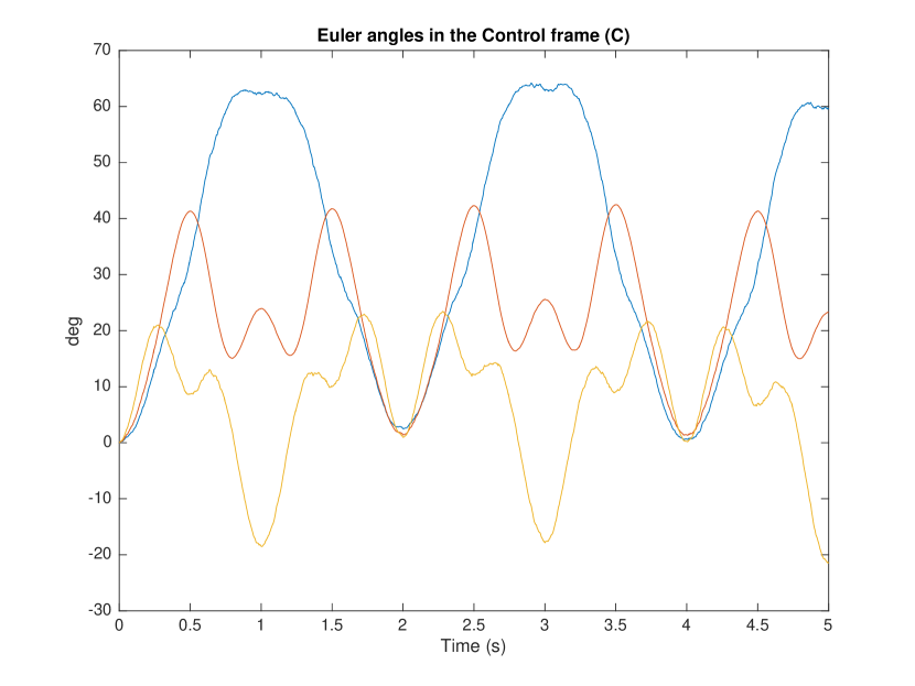
Figure 2: Plot showing the values of the orientation of the IMU in the control frame $\left(\mathcal{C}\right)$ expressed using Euler angles (blue: roll, red: pitch, orange: yaw)

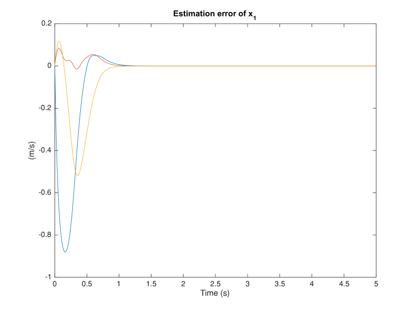
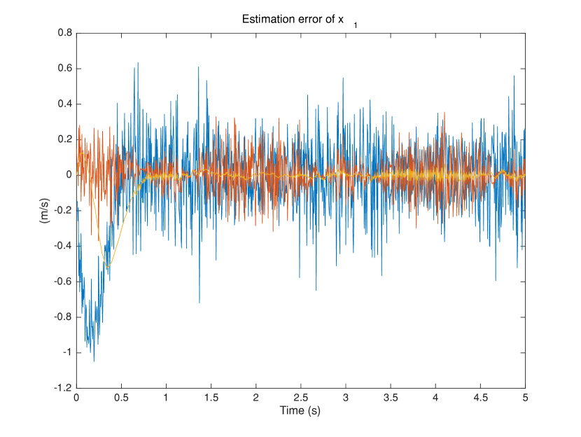
Figure 3: Plot showing the estimation error for $x_{1}$. On the top, the case where there is no noise, and on the bottom the noisy case. The colors blue, red, orange represent the three components of this vector respectively.

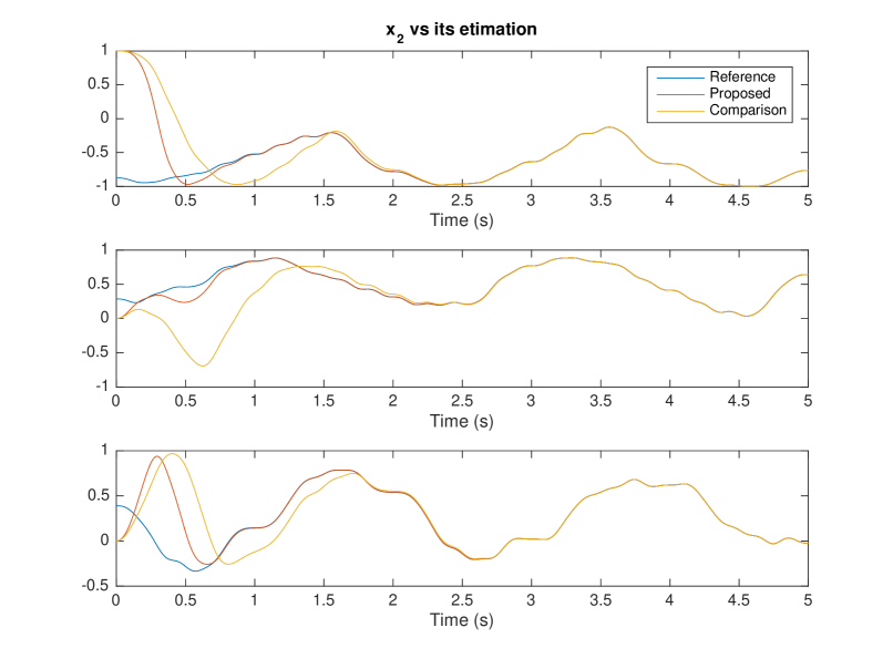
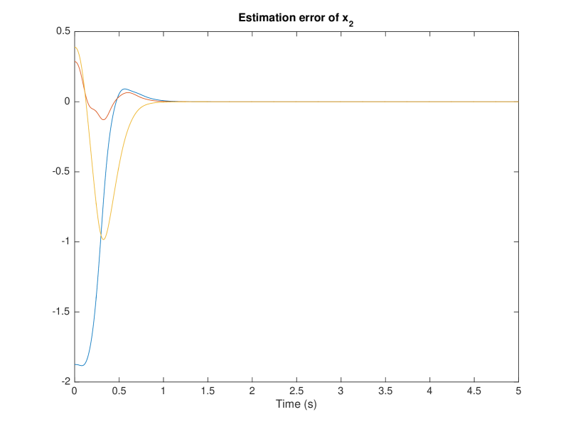
Figure 4: Estimation of $x_{2}$ in the case without noise. On the top, three plots showing a comparison between respective components of $x_{2}$ in blue, its estimation $\hat{x}_{2}$ in red and a comparison with Hua’s observer in yellow. On the bottom we see the evolution of our estimation error. The colors blue, red, orange represent the three components of this vector respectively.

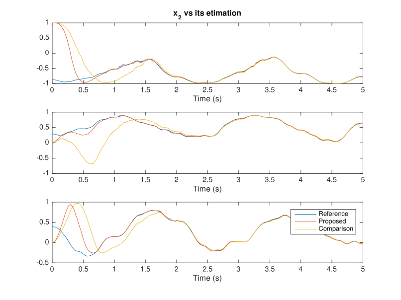
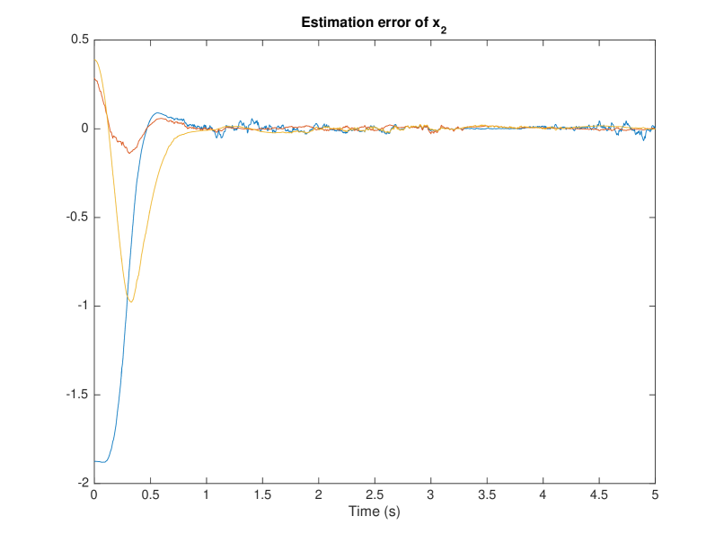
Figure 5: Estimation of $x_{2}$ in the noisy case. On the top, three plots showing a comparison between respective components of $x_{2}$ in blue and its estimation $\hat{x}_{2}$ in red and a comparison with Hua’s observer in yellow. On the bottom we see the evolution of our estimation error $\tilde{x}_{2}$. The colors blue, red, orange represent the three components of this vector respectively.

VI Discussion and conclusion

Attitude estimation is a topic of active research, especially when IMU signals are used. Accelerometers are at the core of this problem mainly because their signal contains the value of the gravitational field in the frame of the sensor. In static cases, this property allows for algebraic tilt measurements. However, in the dynamic cases, this measurement is mixed with the linear acceleration in an algebraically indistinguishable way. In many works the acceleration is considered negligible compared to gravity field [16], and is therefore considered as a noise. Filtering approaches are commonly used to remove this signal [7]. Accelerometers are also commonly used together with gyrometers. Gyrometers provide rotation velocities in the local reference frame. Their signals are commonly merged with accelerometers using Kalman Filtering [8], but are often exploited to correct the filtered accelerometer signals using complementary filtering [9].

Several other works rely on the presence of additional data to reconstruct the attitude. For instance, magnetometers [11] or vision [10] can be used to retrieve redundant attitude signals allowing to reduce the effect of accelerometer errors. Finally, a fusion with external measurements such as GPS [3] or landmark relative position [14] allow to better distinguish the linear acceleration from gravitational field measurements and allows to observe the linear part of the kinematics.

We see through this summary that the translational component of the motion of the IMU is commonly considered either as a noise that requires to be deleted or as an independent dynamics which needs to be observed. However, in the specific case of the pendulum, this linear part of the kinematics is coupled with the angular motion which explains the presence of the angular velocity and event angular acceleration in the signals of the accelerometer (see Equation (4)). This enables us to use this signal without any need of filtering and to still be able to reconstruct tilt despite a high level noise level. The translation-rotation coupling is entirely due to the presence of the anchor point of pivot. However, in several works addressing cases similar to pivot link position estimation are still resorting to classical methods where the IMU is considered as an unconstrained floating object, even if the reconstructed attitude are merged with encoder data afterwards [6]. It is worth to note that in addition to orientation, the orientation estimation of a pendulum provides also data on the position of the limbs of the robot, because of the pivot constraint. This relationship allows also to design position controllers on the base of attitude estimators, similarly to hand position compensation presented in [1].

Only few works dealt with attitude estimation taking into account the pivot constraints. One example is the tilt estimation for rigid pendulum around the pivot using multiple accelerometers [13]. This observer was used especially for balancing the reaction wheel cube on edges and corners [4]. In addition to the requirement of multiple accelerometers at different locations is only limited to rigid pendulum cases. Another work from legged robotics community considers also contact information [2]. This estimator considers the case of multiple contacts and uses an extended Kalman Filter. The contact information is introduced in the model kinematics but only at the prediction step rather than as a constraint. Their model is intended to take into account the cases of contact slippage, but this variable is not observable using inertial sensors. Another work uses also extended Kalman Filtering for a humanoid robot having flexible contacts with the environment [1]. The contact information was introduced as pseudo measurements in order to allow the pivot constraint to be slightly violated. This observer was extended to take into account the dynamical model of the flexibility [12]. However the use of extended Kalman filtering only provides the guarantee of optimality around the linearized dynamics around the predicted state and gives no proof of convergence.

To our knowledge, our estimator is the only one providing almost globally convergent tilt estimation for non-rigid pendulum system. In fact the only work we know which can be adapted to these cases is the observer of [5] where velocity data are used to allow tilt estimation. However, this estimator is more complex than the observer we propose and its convergence properties are weaker, since no minimal set is provided to guarantee the exponential convergence. We could see also that their gain condition for stability lead the system to converge slower than our estimator.

With this kind of estimators the only orientation data missing is the orientation around the gravitational field direction, or yaw angle. This orientation is proven to be out of reach of this measurement system. Therefore, the involvement of other sensors such as magnetometers are necessary to obtain this estimate. The addition of this kind of sensors is the topic of a possible improvement of the presented method.

Finally, the introduction of a model for the dynamics of the pivot could also increase the quality of the observation, specifically by creating coupling between the measurement data of the IMU and other values which are non-observable otherwise. These values include yaw angle without needing additional data, but may go to the estimation of contact forces with the environment [12]. This is also the topic of next developments regarding this kind of systems.

References

- [1] M. Benallegue and F. Lamiraux. Humanoid flexibility deformation can be efficiently estimated using only inertial measurement units and contact information. In International Conference on Humanoid Robots, pages 246–251, 2014.
- [2] M. Bloesch, M. Hutter, M. Hoepflinger, S. Leutenegger, C. Gehring, C. D. Remy, and R. Siegwart. State Estimation for Legged Robots - Consistent Fusion of Leg Kinematics and {IMU}. In Proceedings of Robotics: Science and Systems, Sydney, Australia, 2012.
- [3] F. Caron, E. Duflos, D. Pomorski, and P. Vanheeghe. GPS/IMU data fusion using multisensor Kalman filtering: introduction of contextual aspects. Information fusion, 7(2):221–230, 2006.
- [4] M. Gajamohan, M. Muehlebach, T. Widmer, and R. D ’andrea. The Cubli: A Reaction Wheel Based 3D Inverted Pendulum. 2013.
- [5] M.-D. Hua, P. Martin, and T. Hamel. Stability analysis of velocity-aided attitude observers for accelerated vehicles. Automatica, 63:11–15, jan 2016.
- [6] S. Khandelwal and C. Chevallereau. Estimation of the trunk attitude of a humanoid by data fusion of inertial sensors and joint encoders. In The 16th International Conference on Climbing and Walking Robots, pages 822–830, 2013.
- [7] H. J. Luinge and P. H. Veltink. Inclination measurement of human movement using a 3-D accelerometer with autocalibration. IEEE Transactions on Neural Systems and Rehabilitation Engineering, 12(1):112–121, mar 2004.
- [8] H. J. Luinge, P. H. Veltink, and C. T. M. Baten. Estimation of orientation with gyroscopes and accelerometers. In Proceedings of the First Joint BMES/EMBS Conference., volume 2, page 844, 1999.
- [9] R. Mahony, T. Hamel, and J. M. Pflimlin. Nonlinear Complementary Filters on the Special Orthogonal Group. IEEE Transactions on Automatic Control, 53(5):1203–1218, jun 2008.
- [10] A. Martinelli and R. Siegwart. Vision and IMU Data Fusion: Closed-Form Determination of the Absolute Scale, Speed, and Attitude. In Handbook of Intelligent Vehicles, pages 1335–1354. Springer, 2012.
- [11] N. Metni, J.-M. Pflimlin, T. Hamel, and P. Soueres. Attitude and gyro bias estimation for a VTOL UAV. Control Engineering Practice, 14(12):1511–1520, 2006.
- [12] A. Mifsud, M. Benallegue, and F. Lamiraux. Estimation of Contact Forces and Floating Base Kinematics of a Humanoid Robot Using Only Inertial Measurement Units. In IEEE/RSJ International Conference on Intelligent Robots and Systems, page 6p., sep 2015.
- [13] S. Trimpe and R. D’Andrea. Accelerometer-based tilt estimation of a rigid body with only rotational degrees of freedom. In 2010 IEEE International Conference on Robotics and Automation, pages 2630–2636. IEEE, may 2010.
- [14] J. Fernandes Vasconcelos, R. Cunha, C. Silvestre, and P. Oliveira. A nonlinear position and attitude observer on SE (3) using landmark measurements. Systems & Control Letters, 59(3):155–166, 2010.
- [15] P.-B. Wieber, R. Tedrake, and S. Kuindersma. Springer Handbook of Robotics, chapter Modeling and Control of Legged Robots, pages 1203–1234. Springer International Publishing, Cham, 2016.
- [16] Q. Zheng, Y. Zhang, Y. Lei, J. Song, and Y. Xu. Haircell-inspired capacitive accelerometer with both high sensitivity and broad dynamic range. Proceedings of IEEE Sensors, pages 1468–1473, 2010.