Don’t forget, there is more than forgetting: new metrics for Continual Learning

Abstract

Continual learning consists of algorithms that learn from a stream of data/tasks continuously and adaptively thought time, enabling the incremental development of ever more complex knowledge and skills. The lack of consensus in evaluating continual learning algorithms and the almost exclusive focus on forgetting motivate us to propose a more comprehensive set of implementation independent metrics accounting for several factors we believe have practical implications worth considering in the deployment of real AI systems that learn continually: accuracy or performance over time, backward and forward knowledge transfer, memory overhead as well as computational efficiency. Drawing inspiration from the standard Multi-Attribute Value Theory (MAVT) we further propose to fuse these metrics into a single score for ranking purposes and we evaluate our proposal with five continual learning strategies on the iCIFAR-100 continual learning benchmark.

1 Introduction and Related Work

Catastrophic forgetting (McCloskey and Cohen,, 1989; French,, 1999) refers to the well-known phenomenon of a neural network experiencing a rapid overriding of previously learned knowledge when trained sequentially on new data (McCloskey and Cohen,, 1989). Since, by definition, continual learning algorithms deal with a sequence of data or tasks, eliminating catastrophic forgetting is an important objective often quantified for naturally assessing the quality of novel approaches (Serrà et al.,, 2018; Lopez-Paz and Ranzato,, 2017; Hayes et al.,, 2018; Farquhar and Gal,, 2018). However, the almost exclusive focus on forgetting, motivates us to propose a set of comprehensive metrics for evaluating different factors worth considering in the development of systems that learn continuously, such as accuracy or performance over time, backward and forward knowledge transfer, memory overhead, as well as computational efficiency. For ranking purposes, we also propose a continual learning score ($CL_{score}$) which is flexible enough to be used with different weighting schemes depending on the specific application and needs. The aim of this paper is to stimulate the research community for a more methodical and comprehensive evaluation of continual learning algorithms and convey novel issues and constraints worth considering with respect to “static” machine learning setting.

For an exhaustive evaluation, we can assume to have access to a series of test sets $Te_{i}$ over time. The aim is to assess and disentangle the performance of our learning hypothesis $h_{i}$ as well as to evaluate if it is representative of the knowledge that should be learned by the correspondent training batch $Tr_{i}$. However, as discussed in (Lopez-Paz and Ranzato,, 2017), a different granularity of the evaluation at the task level can as well be achieved by having the same test batch for many $Tr_{i}$.

An overall performance $\Omega$ in a supervised classification setting was proposed in (Hayes et al.,, 2018) based on the relative performance of an incrementally trained algorithm with respect to an off-line trained one (which has access to all the data at once, and acts as an upper bound). Serrà et al., (2018), instead, try to directly model forgetting with a proposed forgetting ratio metric $\rho$ that considers a vector of test accuracies for each $Te_{i}$ at random initialization that represents a lower bound on accuracy. In the same setting, in (Lopez-Paz and Ranzato,, 2017) other three important metrics are proposed: Average Accuracy (ACC), Backward Transfer (BWT), Forward Transfer (FWT). In this case, after the model finishes learning about the training set $Tr_{i}$, its performance is evaluated on all (even future) test batches. The higher these metrics, the better the model. If two models have similar ACC, the most preferable one is the one with larger BWT and FWT. While forgetting and knowledge transfer could be quantified and evaluated in various ways (Farquhar and Gal,, 2018; Hayes et al.,, 2018), these may not suffice for a robust evaluation of CL strategies in practice. We thus propose a comprehensive set of metrics that expands and complements existing ones.

2 Proposed Metrics for Continual Learning

In Continual Learning, $\mathcal{D}$ can be thought of a potentially infinite sequence of unknown distributions $\mathcal{D}=\{D_{1},\dots,D_{n}\}$ over $X\times Y$ we encounter over time, with $X$ and $Y$ as input and output random variables respectively. Given $h^{*}$ as the general target function (i.e. our ideal prediction model), a task $T$ is defined by a unique task label $t$ and its target function $g_{\hat{t}}^{*}(x)\equiv h^{*}(x,t=\hat{t})$, i.e., the objective of its learning. A CL algorithm $A^{CL}$ is an algorithm with the following signature:

$$\forall D_{i}\in\mathcal{D},\hskip 20.0ptA^{CL}_{i}:\ \ <h_{i-1},Tr_{i},M_{i-1},t>\rightarrow<h_{i},M_{i}>$$ (1)

Where $h_{i}$ is the model, $Tr_{i}$ is the training set of examples drawn from the respective $D_{i}$ distribution, $M_{i}$ is an external memory where we can store previous training examples and $t$ is a task label. For simplicity, we can assume $N$ as the number of tasks, one for each $Tr_{i}$.

In this CL framework, we propose algorithm ranking metrics according to different desiderata attainable in CL divided on seven criteria. In order to provide bounds to each metric (originally lying in $f:[0,\infty[$), we map it to a $[0,1]$ range (as it is commonly done, e.g., in Multi-Attribute Value Theory (MAVT) (Keeney and Raiffa,, 1993)) and formulate it so that its optimal value is given by its maximization. This is to preserve interpretability of the proposed aggregating $CL_{score}$ metric, and allow to evaluate CL algorithms with respect to multiple criteria, rank them from best to worst, and accommodate weighting schemes according to constraints and desiderata.

Accuracy: Given the train-test accuracy matrix $R\in\mathds{R}^{N\times N}$, which contains in each entry $R_{i,j}$ the test classification accuracy of the model on task $t_{j}$ after observing the last sample from task $t_{i}$ (Lopez-Paz and Ranzato,, 2017), Accuracy (A) considers the average accuracy for training set $Tr_{i}$ and test set $Te_{j}$ by considering the diagonal elements of $R$, as well as all elements below it (see Table 2):

$$A=\frac{\sum_{i\geq j}^{N}R_{i,j}}{\frac{N(N+1)}{2}}$$ (2)

While the A criteria was originally defined to asses the performance of the model at the end of the last task (Lopez-Paz and Ranzato,, 2017), we believe that an accuracy metric that takes into account the performance of the model at every timestep i in time better characterizes the dynamic aspects of CL. The same idea is applied to the modified BWT and FWT metrics introduced below.

Backward Transfer (BWT) measures the influence that learning a task has on the performance on previous tasks (Lopez-Paz and Ranzato,, 2017). The motivation arises when an agent needs to learn in a multi-task or data stream setting. The lifelong abilities to both improve and not degrade performance are important and should be evaluated throughout its lifetime. It is defined as the accuracy computed on $Te_{i}$ right after learning $Tr_{i}$ as well as at the end of the last task on the same test set. (see Table 2). Here, as in the accuracy metric, we expand it to consider the average of the backward transfer after each task:

$$BWT=\frac{\sum_{i=2}^{N}\sum_{j=1}^{i-1}(R_{i,j}-R_{j,j})}{\frac{N(N-1)}{2}}$$ (3)

Because the original meaning of BWT assumed positive values for backward transfer and negative values to define (catastrophic) forgetting, in order to map BWT to also lie on $[0,1]$ and give more importance to two semantically different concepts, BWT is broken into two different clipped terms: The originally negative (forgetting) BWT (now positive), i.e., Remembering, as $REM=1-|min(BWT,0)|$. and (the originally positive) BWT, i.e., improvement over time Positive Backward Transfer $BWT^{+}=max(BWT,0)$.

Forward Transfer: FWT measures the influence that learning a task has on the performance of future tasks (Lopez-Paz and Ranzato,, 2017). Following the spirit of the previous metrics we modify it as the average accuracy for the train-test accuracy entries $R_{i,j}$ above the principal diagonal of R, excluding it (see elements accounted in Table 2 in light gray and additional information in the appendix). Forward transfer can occur when the model is able to perform zero-shot learning. We therefore redefine FWT as:

$$FWT=\frac{\sum_{i<j}^{N}R_{i,j}}{\frac{N(N-1)}{2}}$$ (4)

Model size efficiency: The memory size of model $h_{i}$ quantified in terms of parameters $\theta$ at each task $i$, $Mem(\theta_{i})$, should not grow too rapidly with respect to the size of the model that learned the first task, $Mem(\theta_{1})$. Model size (MS) is thus:

$$MS=min(1,\frac{\sum_{i=1}^{N}\frac{Mem(\theta_{1})}{Mem(\theta_{i})}}{N})$$ (5)

Samples storage size efficiency: Many CL approaches save training samples as a replay strategy to not forget. The memory occupation in bits by the samples storage memory $M$, $\mathit{Mem}(M)$, should be bounded by the memory occupation of the total number of examples encountered at the end of the last task, i.e. the cumulative sum of $Tr_{i}$ here defined as the lifetime dataset $D$ (associated to the set of all distributions $\mathcal{D}$). Thus, we define Samples Storage Size (SSS) efficiency as:

$$SSS=1-min(1,\frac{\sum_{i=1}^{N}\frac{\mathit{Mem}(M_{i})}{\mathit{Mem}(D)}}{N})$$ (6)

Computational efficiency: Since the computational efficiency (CE) is bounded by the number of multiplication and addition operations for the training set $Tr_{i}$, we can define the average CE across tasks as:

$$CE=min(1,\frac{\sum_{i=1}^{N}\frac{\mathit{Ops}\uparrow\downarrow(Tr_{i})\cdot\varepsilon}{\mathit{Ops}(Tr_{i})}}{N})$$ (7)

where $Ops(Tr_{i})$ is the number of (mul-adds) operations needed to learn $Tr_{i}$, and $Ops\uparrow\downarrow$($Tr_{i}$) is the number of operations required to do one forward and one backward (backprop) pass on $Tr_{i}$. When the value of $Ops\uparrow\downarrow$($Tr_{i}$) is negligible w.r.t. $Ops(Tr_{i})$, a scaling factor associated to the number of epochs needed to learn $Tr_{i}$, $\varepsilon$ larger than a default value of 1, can be used to make CE more meaningful (i.e. avoiding compression of the values very near to zero). Since we are essentially moving the lower bound of the computation, which depends on the benchmark complexity, this adjustment also translates on better interpretability of CE (Fig. 1)

In order to assess a CL algorithm $A^{CL}$, following (Ishizaka and Nemery,, 2013), each criterion $c_{i}\in\mathcal{C}$ (where $c_{i}\in[0,1]$) is assigned a weight $w_{i}\in[0,1]$ where $\sum_{i}^{\mathcal{C}}w_{i}=1$. Each $c_{i}$ should be the average of $r$ runs. Therefore, the final $CL_{score}$ to maximize is computed as:

$$CL_{score}=\sum_{i=1}^{\#\mathcal{C}}w_{i}c_{i}$$ (8)

where each criterion $c_{i}$ that needs to be minimized is transformed to $c_{i}=1-c_{i}$ to preserve increasing monotonicity of the metric (for overall maximization of all criteria in $\mathcal{C}$). $CL_{stability}$ is thus:

$$CL_{stability}=1-\sum_{i=1}^{\#\mathcal{C}}w_{i}\mathit{stddev}(c_{i})$$ (9)

3 Experiments and Conclusions

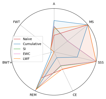
Figure 1: a) Spider chart: CL metrics per strategy (larger area is better). b) Accuracy per CL strategy computed over the fixed test set as proposed in (Lomonaco and Maltoni,, 2017; Maltoni and Lomonaco,, 2018).

We evaluate the CL metrics on cumulative and naïve baseline strategies as in (Maltoni and Lomonaco,, 2018), Elastic Weight Consolidation (EWC) (Kirkpatrick et al.,, 2016), Synaptic Intelligence (SI) (Zenke et al.,, 2017) and Learning without Forgetting (LwF) (Li and Hoiem,, 2016). iCIFAR-100 (Rebuffi et al.,, 2018) dataset is used: each task consists of a training batch of 10 (disjoint) classes at a time.

Results for each proposed metric are illustrated in Table 1 (each criterion $c_{i}$ reports the average over 3 runs); Fig. 1 illustrates the CL metrics variability for each criterion reflecting a desirable property of CL algorithms, as well as the needs of novel techniques addressing different aspects than accuracy and forgetting, that can be important depending on the application. For simplicity, we chose an homogeneous configuration of criteria weights that values each CL metric equally (i.e., each $w_{i}=\frac{1}{\#\mathcal{C}}$). However, the Appendix shows results on other possible configurations.

While the $CL_{score}$ is optional to report, the aim of the metrics and results is to stimulate comprehensive evaluation practices. In future work we plan to refine these metrics and assess more strategies in more exhaustive evaluation settings.

Table 1: CL metrics and $CL_{score}$ for each CL strategy evaluated (higher is better).

Strategy	A	REM	BWT+	FWT	MS	SSS	CE	$\bm{CL_{score}}$	$\bm{CL_{stability}}$
Naïve	0.3825	0.6664	0.0000	0.1000	1.0000	1.0000	0.4492	0.5140	0.9986
Cumul.	0.7225	1.0000	0.0673	0.1000	1.0000	0.5500	0.1496	0.5128	0.9979
EWC	0.5940	0.9821	0.0000	0.1000	0.4000	1.0000	0.3495	0.4894	0.9972
LWF	0.5278	0.9667	0.0000	0.1000	1.0000	1.0000	0.4429	0.5768	0.9986
SI	0.5795	0.9620	0.0000	0.1000	0.4000	1.0000	0.3613	0.4861	0.9970

4 Acknowledgements

We acknowledge Matteo Brunelli and Dmitry Ponomarev for their brainstorm support.

Appendix A Implementation Details

A.1 Metrics and benchmark illustration

Table 2: Elements in $R$ accounted to compute the Accuracy (white and cyan elements), BWT (in cyan), and FWT (in light gray) criteria. $R^{*}=R_{ii}$, $Tr_{i}$ = training, $Te_{i}$= test tasks.

R	$Te_{1}$	$Te_{2}$	$Te_{3}$
$Tr_{1}$	$R^{*}$	$R_{ij}$	$R_{ij}$
$Tr_{2}$	$R_{ij}$	$R^{*}$	$R_{ij}$
$Tr_{3}$	$R_{ij}$	$R_{ij}$	$R^{*}$

Matrix $R\in\mathds{R}^{N\times N}$ contains in each entry $R_{i,j}$ the test classification accuracy of the model on task $j$ after observing the last sample from task $i$ (Lopez-Paz and Ranzato,, 2017). $N$ is the number of tasks; here for simplicity we make the number of distributions $n$ equal to $N$. Table 2 shows the elements in the accuracy matrix used for each metric for an example matrix of $N=3$ tasks. $R^{*}=R_{ii}$ coincides with the (normally) optimal accuracy right after using training set $Tr_{i}$ and testing on test set $Te_{i}$.

Note that in order to compute Accuracy, we do not only consider as (Lopez-Paz and Ranzato,, 2017) the last row of the accuracy matrix $R$, but also steps in between each new training set learned, to acknowledge the degradation and improvement through every time step in time.

In FWT, the substraction term (vector $b_{i}$ of test accuracies for each task at random initialization) in the original FWT formula in (Lopez-Paz and Ranzato,, 2017) was removed in our definition of FWT in order to guarantee non negative values (i.e. in case of negative FWT) and allow for potential positive transfer, as they demonstrate it is possible to happen with a shared output space. The idea is supporting the fact that algorithms can do worse than random accuracy for some strategies (we refer the reader to (Lopez-Paz and Ranzato,, 2017) for cases of positive FWT).

The original BWT (Lopez-Paz and Ranzato,, 2017) would return domains for $BWT^{-}\in[0,0.5)$, and for $BWT^{+}\in[0.5,1]$, respectively which, through the clipping, are transformed, as the rest of criteria in the CL metric, to stay in [0,1].

Criteria weights setting and experiments Despite the experiments showing the $CL_{score}$ to be optional and context dependent; the aggregation score is most meaningful when a community agrees on a particular evaluation criteria (similarly to the mAP metric), or in specific settings where the weights for the different criteria are clearly definable. Our experiments use three weight configurations $W$ = [$w_{A},w_{MS},w_{SSS},w_{CE},w_{BWT},w_{Rem},w_{FWT}$]. The first one used homogeneous weights (each $w_{i}=\frac{1}{\#\mathcal{C}}$) and the second and third use $W_{2}$ = [0.4, 0.1, 0.1, 0.1, 0.2, 0.05, 0.05] and $W_{3}$ = [0.4, 0.05, 0.2, 0.2, 0.05, 0.05, 0.05], as particular examples aiming at reflecting what the recent CL literature has roughly been valuing the most; however, any configuration could be used.

Model: The CNN model used in this experiment is the same used in (Zenke et al.,, 2017) and (Maltoni and Lomonaco,, 2018) and consists of 4 convolutional + 2 fully connected layers (details available in Appendix A of (Zenke et al.,, 2017)). Hyper-parameters are chosen to maximize the accuracy metric $A$ for each strategy.

Benchmark: CIFAR-100 (Krizhevsky,, 2009) classification dataset has 100 classes containing 600 natural images (32$\times$32) each (500 training + 100 test). The CL setting of iCIFAR-100 splits the 100 classes in groups. In this paper we consider groups of 10 classes, and therefore obtain 10 incremental batches.

Baselines: The lower and upper bound CL strategies are naïve and cumulative learning, respectively. The naïve learning strategy starts at $Tr_{1}$ and learns continuously the coming training sets $Tr_{2},...,Tr_{N}$ simply tuning the model across batches without any specific mechanism to control forgetting, except early stopping. The cumulative strategy starts from scratch every time, learning from the accumulation of $Tr_{1},...,Tr_{i-1},Tr_{i}$ retrained with the patterns from the current batch and all previous batches (only in this approach we assume that all previous data can be stored and reused). This cumulative method is a sort of upper bound, or ideal performance that CL strategies should try to reach (Maltoni and Lomonaco,, 2018).

Spider chart in Fig 1 shows all objective criteria, where the larger the area occupied under the CL algorithm curve, the highest $CL_{score}$ (more optimal) it is. Fig. 2 shows each of the main CL strategies put in context compared with the considered lower and upper bounds respectively, i.e., naïve, and cumulative strategies. The farther away the evaluated strategy is from the cumulative (blue) surface, the larger room for improvement for the CL strategy.

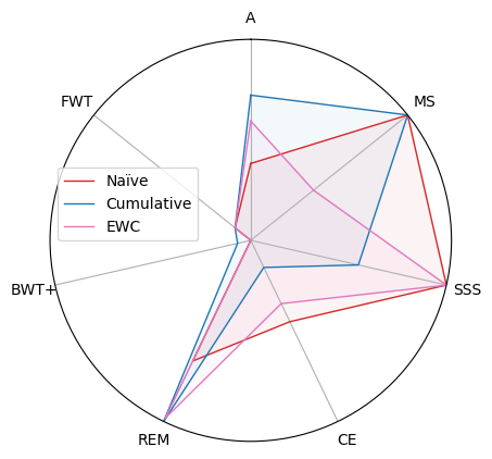
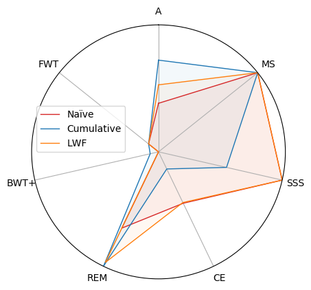
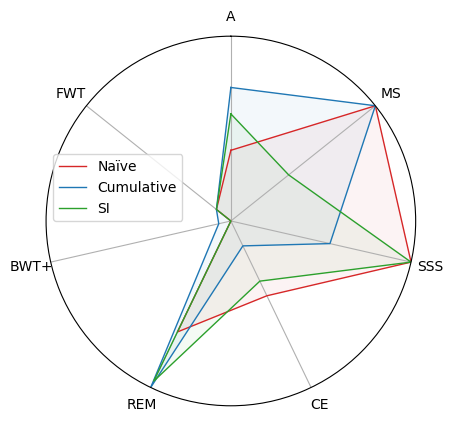
Figure 2: Spider chart with CL metrics showing CL strategies EWC, LWF and SI with their respective lower and upper bound (Naïve and Cumulative resp.) as reference baselines (to properly visualize Fig. 1). The weight configuration for each criterion used is $W_{1}$ where $w_{i}=\frac{1}{7}$ for each $w_{i}\in W$.

Table 3: $CL_{score}$ and $CL_{stability}$ for all CL strategies according to different weighting configurations $W_{i}$ = [$w_{A},w_{MS},w_{SSS},w_{CE},w_{REM^{+}},w_{BWT},w_{FWT}$], where $W_{1}$ sets $w_{i}=\frac{1}{7}$ for each $w_{i}\in W$. The second setting of a concrete metric weights is $W_{2}$ = [0.4, 0.05, 0.2, 0.1, 0.15, 0.05, 0.05]. A third arbitrary configuration is $W_{3}$ = [0.4, 0.05, 0.2, 0.2, 0.05, 0.05, 0.05].

Strategy/CL Metric	$\bm{CL_{score}}$			$\bm{CL_{stability}}$
	$W_{1}$	$W_{2}$	$W_{3}$	$W_{1}$	$W_{2}$	$W_{3}$
Naïve	0.5140	0.5529	0.5312	0.9986	0.9969	0.9973
Cumulative	0.5128	0.6223	0.5373	0.9979	0.9976	0.9964
EWC	0.4894	0.6449	0.5816	0.9972	0.9976	0.9940
LWF	0.5768	0.6554	0.6030	0.9986	0.9990	0.9972
SI	0.4861	0.6372	0.5772	0.9970	0.9945	0.9927

References

- Farquhar and Gal, (2018) Farquhar, S. and Gal, Y. (2018). Towards robust evaluations of continual learning. arXiv preprint arXiv:1805.09733.
- French, (1999) French, R. M. (1999). Catastrophic forgetting in connectionist networks. Trends in Cognitive Sciences, 3(4):128–135.
- Hayes et al., (2018) Hayes, T. L., Cahill, N. D., and Kanan, C. (2018). New Metrics and Experimental Paradigms for Continual Learning. pages 1–4.
- Ishizaka and Nemery, (2013) Ishizaka, A. and Nemery, P. (2013). Multi-criteria decision analysis: methods and software. John Wiley & Sons.
- Keeney and Raiffa, (1993) Keeney, R. and Raiffa, H. (1993). Decision with multiple objectives, preferences and value tradeoffs.
- Kirkpatrick et al., (2016) Kirkpatrick, J., Pascanu, R., Rabinowitz, N., Veness, J., Desjardins, G., Rusu, A. A., Milan, K., Quan, J., Ramalho, T., Grabska-Barwinska, A., Hassabis, D., Clopath, C., Kumaran, D., and Hadsell, R. (2016). Overcoming catastrophic forgetting in neural networks. ArXiv e-prints.
- Krizhevsky, (2009) Krizhevsky, A. (2009). Learning Multiple Layers of Features from Tiny Images. PhD thesis.
- Li and Hoiem, (2016) Li, Z. and Hoiem, D. (2016). Learning without Forgetting. ArXiv e-prints.
- Lomonaco and Maltoni, (2017) Lomonaco, V. and Maltoni, D. (2017). Core50: a new dataset and benchmark for continuous object recognition. In Levine, S., Vanhoucke, V., and Goldberg, K., editors, Proceedings of the 1st Annual Conference on Robot Learning, volume 78 of Proceedings of Machine Learning Research, pages 17–26. PMLR.
- Lopez-Paz and Ranzato, (2017) Lopez-Paz, D. and Ranzato, M. (2017). Gradient Episodic Memory for Continual Learning. ArXiv e-prints.
- Maltoni and Lomonaco, (2018) Maltoni, D. and Lomonaco, V. (2018). Continuous learning in single-incremental-task scenarios. arXiv preprint arXiv:1806.08568.
- McCloskey and Cohen, (1989) McCloskey, M. and Cohen, N. J. (1989). Catastrophic interference in connectionist networks: The sequential learning problem. In Psychology of learning and motivation, volume 24, pages 109–165. Elsevier.
- Rebuffi et al., (2018) Rebuffi, S.-A., Bilen, H., and Vedaldi, A. (2018). Efficient parametrization of multi-domain deep neural networks. pages 8119–8127.
- Serrà et al., (2018) Serrà, J., Surís, D., Miron, M., and Karatzoglou, A. (2018). Overcoming catastrophic forgetting with hard attention to the task. CoRR, abs/1801.01423.
- Zenke et al., (2017) Zenke, F., Poole, B., and Ganguli, S. (2017). Continual learning through synaptic intelligence. In Precup, D. and Teh, Y. W., editors, Proceedings of the 34th International Conference on Machine Learning, volume 70 of Proceedings of Machine Learning Research, pages 3987–3995, International Convention Centre, Sydney, Australia. PMLR.