Planar $N$-body central configurations with a homogeneous potential

Abstract.

Central configurations give rise to self-similar solutions to the Newtonian $N$-body problem, and play important roles in understanding its complicated dynamics. Even the simple question of whether or not there are finitely many planar central configurations for $N$ positive masses remains unsolved in most cases. Considering central configurations as critical points of a function $f$, we explicity compute the eigenvalues of the Hessian of $f$ for all $N$ for the point vortex potential for the regular polygon with equal masses. For homogeneous potentials including the Newtonian case we compute bounds on the eigenvalues for the regular polygon with equal masses, and give estimates on where bifurcations occur. These eigenvalue computations imply results on the Morse indices of $f$ for the regular polygon. Explicit formulae for the eigenvalues of the Hessian are also given for all central configurations of the equal mass 4-body problem with a homogeneous potential. Classic results on collinear central configurations are also generalized to the homogeneous potential case. Numerical results, conjectures, and suggestions for future work in the context of a homogeneous potential are given.

1. Introduction

The classical dynamics of $N$ point particles with masses $m_{i}$ interacting via a central potential $U$ are given by:

$$m_{i}\ddot{q}_{i;j}=\frac{\partial U}{\partial q_{i;j}},\ \ i\in\{0,\ldots N-1\},\ \ j\in\{1,\ldots,d\}$$

where $q_{i}\in\mathbf{R}^{d}$ is the position of particle $i$ with components $q_{i;j}$, and

$$U=\sum_{i<k}m_{i}m_{k}/r_{i,k}^{A-2}$$

is the potential with a real parameter $A>2$, and $r_{i,k}$ is the distance between $q_{i}$ and $q_{k}$. The case of Newtonian gravity is $A=3$ [103], and provides the primary motivation for studying this more general problem. We can extend this potential to the case $A=2$ by using the logarithmic potential

$$U=\sum_{i<k}m_{i}m_{k}\log(r_{i,k})$$

which arises in a simplified model of fluid vortices [64, 69, 13]. In the vortex model case the parameters $m_{i}$ represent the strength of a vortex rotation, and can be any real value. However our main interest is the Newtonian case, for which we usually assume non-negative mass parameters.

In this article we focus our attention on configurations with the special property that each particle is accelerated towards the center of mass of the system at a rate uniformly proportional to its distance from the center of mass, i.e.

$$m_{i}\ddot{q}_{i;j}=\lambda(q_{i;j}-q_{C,j})$$

with $q_{C}=\frac{1}{M}\sum m_{i}q_{i}$ the center of mass, and $M=\sum m_{i}$ is the total mass. Such configurations are called central configurations (as well as permanent or stationary configurations in some older literature). In the planar case they also account for the relative equilibria, which are equilibria in a uniformly rotating reference frame. Central configurations are important in the $N$-body problem for a number of reasons, including the study of multiple body collisions [89, 67, 38, 93] and the topology of the phase space for a fixed energy [25, 40, 1, 88]. Understanding of the dynamics near central configurations was critical in the proof of chaotic behavior in the three-body problem [94].

For more background on central configurations we highly recommend the recent summary by Moeckel [99], as well as earlier surveys [119, 95, 41, 70, 120].

A longstanding open problem about central configurations is whether or not there are finitely many equivalence classes of central configurations for a particular choice of $N$ positive masses (usually restricted to the Newtonian case of $A=3$). The most famous version of this problem further restricts the configurations to $\mathbf{R}^{2}$, and was highlighted by Stephen Smale as the sixth of his ‘Mathematical problems for the next century’ [134]. Smale himself considered the problem [132, 133], and introduced a topological viewpoint that we will consider in the next section. This problem was also formulated earlier by Wintner [140] and Chazy [28], and highlighted more recently in [6]. We follow the usual convention of considering two planar configurations equivalent if there is a direct isometry between them (i.e. an orientation-preserving rigid motion).

The difficulty of the finiteness problem was underscored by the discovery of a counter-example in the 5-body problem if a negative mass is allowed [112]. This example has been extended to more general settings [52]. The existence of positive dimensional sets of central configurations for some negative mass parameters makes many approaches using algebraic geometry challenging, since methods based on complex varieties are incapable of ruling these out. Indeed, although there have been numerous successful applications of methods from classical and real algebraic geometry and tropical geometry to the finiteness problem [98, 74, 61, 62, 57, 59, 10], we believe that solving the finiteness problem in general requires additional tools.

The primary hypothesis of this manuscript is that studying the central configurations for a homogeneous potential (more general than the Newtonian) will more naturally develop mathematical tools that will advance the Newtonian case, analogously to the use of tools from complex analysis in solving real-analytic problems (e.g. contour integrals). In particular we believe it would be valuable to develop a framework for central configurations in the limiting case of $A\rightarrow\infty$.

In what follows we consider central configurations as critical points of the function

$$f=\frac{MI}{2}+\frac{U}{A-2},$$

where $I$ is the moment of inertia

$$I=\sum_{i=1}^{N}m_{i}r_{i}^{2}$$

where $r_{i}=|q_{i}|$ is the distance from the $i$th point to the origin. If the center of mass is at the origin, then

$$I=\frac{1}{M}\sum_{i<j}m_{i}m_{j}r_{i,j}^{2}.$$

Because the potential function $U$ is invariant under translation, all critical points of $f$ will have their center of mass at the origin. In contrast to some other formulations of central configurations, our $f$ is homogeneous in the mass parameters but not in the distance variables. We have in effect set a preferred scale from the beginning in order to have an unconstrained problem. We find this approach simplest, but there are many other formulations of the problem [73, 4, 99, 48].

The idea of studying a more general potential, even if we are mainly interested in the Newtonian case, is an old one [136, 71, 4, 8, 33]. We would like to especially highlight the study of the behavior of central configurations for large values of $A$, which has not recieved much attention in the literature before.

We briefly review the relevant topology for using Morse theory in the $N$-body problem.

The configuration space we will use is $\mathcal{C}_{N}=(\mathbb{R}^{2N}\backslash\Delta)/S^{1}$, where $\Delta$ is the subset of collisions ($q_{i}=q_{j}$ for $i\neq j$) and the quotient is taken with respect to proper rotations around the origin treating $\mathbb{R}^{2N}$ as $(\mathbb{R}^{2})^{N}$. The function $f$ is well-defined on this quotient since both $I$ and $U$ are rotationally invariant.

The simplest versions of Morse theory concern the behavior of a smooth function on a compact manifold, with the extra condition that the critical points of the function are nondegenerate (i.e. the Hessian is nondegenerate). Although our function $f$ is not defined on a compact manifold (because of the removal of the set $\Delta$), this can be remedied without too much effort because the gradient of $f$ will always become outward pointing close to $\Delta$. This was made precise by Shub [129]. Assuming $f$ is nondegenerate, its level sets change in topology at each critical value. If the topology of the manifold is non-trivial, such changes in the level sets are inevitable. The index of a critical point is the dimension of the largest subspace on which the Hessian of $f$ is negative definite. Let the number of critical points with index $j$ be $n_{j}$, and encode this information in the Morse polynomial:

$$M(t)=\sum_{j=0}^{dim(\mathcal{C}_{N})}n_{j}t^{j}$$

where $t$ is an auxiliary variable. The Poincaré polynomial for a manifold is defined as $P(t)=\sum\beta_{j}t^{j}$, where $\beta_{j}$ is the $j$th Betti number. Morse theory relates these polynomials by

$$M(t)=P(t)+(1+t)R(t),$$

where $R(t)$ is a polynomial with non-negative integer coefficients. This not only puts a lower bound on the number of critical points, but also provides constraints on the possible $n_{j}$.

For more background on Morse theory we recommend [92, 21].

The Poincaré polynomial for the manifold $\mathcal{C}_{N}$ is $P_{N}(t)=\prod_{j=1}^{N-1}(1+jt)$ [16]. The corresponding result in the spatial case was first computed in [105]; in dimension $d$, $P_{N,d}(t)=\prod_{j=1}^{N-1}(1+jt^{d-1})$ [99].

It is not completely clear how much the index of a critical point influences the more general dynamical behavior of orbits near the central configuration, although there are some results connecting these [66, 20]. Not many cases of exact calculations of linear stability are available. The general problem was made precise by Andoyer [12]. Particular cases have been studied for three bodies [50, 117, 115, 121], four bodies [111, 22, 116, 135], restricted cases (i.e. with one or more infinitesimal masses) [107], and polygonal and $N+1$ ring systems [53, 125, 96, 114, 26, 19]; more could be done, especially numerically, in our setting of a variable exponent potential. A particularly interesting example is the lower bound for instability of equal mass relative equilbria found by Roberts [113] in the Newtonian case.

A recent result of Montaldi [101] uses only the existence of a minimum of $f$ to derive the existence of a large family of symmetric central configurations; in many settings this result could be strengthened using Morse theory (assuming the function $f$ is non-degenerate). The existing upper and lower bounds for central configurations are far from sharp, despite some substantial effort [80, 87, 90, 5].

2. The regular polygon in the N-body problem

We can prove some properties of the Morse index of central configurations for the regular polygon in the $N$-body problem for varying $A$, and speculate on some others. Quite a few results for regular polygon central configurations are known for the Newtonian ($A=3$) and vortex $(A=2)$ cases [85, 109, 91, 27].

These configurations are well suited to polar coordinates, so we will express the position of the $i$th particle as

$$q_{i}=(r_{i}\cos(\theta_{i}),r_{i}\sin(\theta_{i}))$$

For the regular polygon centered at the origin, all of the radii are equal ($r_{i}=r$ for some $r$) and $\theta_{i}=\frac{2\pi i}{N}$ where we will index the particles starting at $i=0$. In what follows we denote the evaluation of a function at the equal mass regular polygon by a superscript circle, e.g. $f^{\circ}$. For the interparticles distances we define $p_{i,j}=ru_{i,j}=(r_{i,j})^{\circ}$, where

$$u_{i,j}=\sqrt{2-2\cos\left[\frac{2\pi(j-i)}{N}\right]}=2\sin(\frac{\pi|j-i|}{N})$$

are the distances between points $i$ and $j$ on the unit radius regular polygon.

As before we consider central configurations as critical points of the function $f=\frac{MI}{2}+\frac{U}{A-2}$. To calculate derivatives of $f$ we will need the partial derivatives of the interparticle distances with respect to $r_{i}$ and $\theta_{i}$:

$$\frac{\partial r_{i,j}}{\partial r_{i}}=\frac{r_{i}-r_{j}\cos(\theta_{j}-\theta_{i})}{r_{i,j}}$$

$$\frac{\partial r_{i,j}}{\partial\theta_{i}}=\frac{-r_{i}r_{j}\sin(\theta_{j}-\theta_{i})}{r_{i,j}}.$$

Evaluated on the regular polygon, we have

$$\left(\frac{\partial r_{i,j}}{\partial r_{i}}\right)^{\circ}=\frac{1-\cos(\theta_{j}-\theta_{i})}{u_{i,j}}=u_{i,j}/2$$

$$\left(\frac{\partial r_{i,j}}{\partial\theta_{i}}\right)^{\circ}=-r\frac{\sin(\theta_{j}-\theta_{i})}{u_{i,j}}=-r\cos\left(\frac{\pi|j-i|}{N}\right).$$

The gradient of $f$ with respect to $r_{i}$ and $\theta_{i}$ has components

$$\frac{\partial f}{\partial r_{i}}=m_{i}Mr_{i}-m_{i}\sum_{j\neq i}m_{j}r_{i,j}^{-A}(r_{i}-r_{j}\cos(\theta_{j}-\theta_{i}))$$

and

$$\frac{\partial f}{\partial\theta_{i}}=m_{i}\sum_{j\neq i}m_{j}r_{i,j}^{-A}r_{i}r_{j}\sin(\theta_{j}-\theta_{i}).$$

Evaluated at the equal mass regular polygon these are

$$\left(\frac{\partial f}{\partial r_{i}}\right)^{\circ}=Nr-r\sum_{j\neq i}p_{i,j}^{-A}(1-\cos(\theta_{j}-\theta_{i}))$$

$$\left(\frac{\partial f}{\partial\theta_{i}}\right)^{\circ}=r^{2}\sum_{j\neq i}p_{i,j}^{-A}\sin(\theta_{j}-\theta_{i})=0.$$

where the second quantity is zero because $\sin(t)$ is odd and $p_{i,j}$ is even.

To be a critical point of $f$, $(\frac{\partial f}{\partial r_{0}})^{\circ}=0$, which can be solved for the radius:

$$r=\left(\frac{\sum_{j=1}^{N-1}u_{0,j}^{2-A}}{2N}\right)^{1/A}$$

As $A$ increases, this radius increases to the limit value $r_{\infty}(N)=(2\sin(\pi/N))^{-1}$, for which $p_{i,i+1}=1$. For $A=2$, the radius is equal to $\sqrt{\frac{N-1}{2N}}$.

Now to compute the Morse index of $f$ for regular polygons we need the components of the Hessian of $f$. In expressions involving indices $i$ and $j$, it is assumed that $i\neq j$. In the final form shown for each expression we use the radius $r$ and unit polygon distances $u_{i,j}$ as much as possible.

$$\frac{\partial^{2}f}{\partial r_{i}\partial r_{j}}=m_{i}m_{j}r_{i,j}^{-A-2}\left(A(r_{i}-r_{j}\cos(\theta_{j}-\theta_{i}))(r_{j}-r_{i}\cos(\theta_{j}-\theta_{i}))+r_{i,j}^{2}\cos(\theta_{j}-\theta_{i})\right)$$

$$R_{i,j}:=\left(\frac{\partial^{2}f}{\partial r_{i}\partial r_{j}}\right)^{\circ}=p_{i,j}^{-A}\left[\frac{A}{2}(1-\cos\left(\frac{2\pi(j-i)}{N}\right))+\cos\left(\frac{2\pi(j-i)}{N}\right)\right]$$

which simplifies to

$$R_{i,j}=r^{-A}u_{i,j}^{-A}\left(u_{i,j}^{2}\frac{A-2}{4}+1\right)$$

$$\frac{\partial^{2}f}{\partial r_{i}^{2}}=m_{i}(M-\sum_{j\neq i}m_{j}r_{i,j}^{-A-2}\left[r_{i,j}^{2}-A(r_{i}-r_{j}\cos(\theta_{j}-\theta_{i}))^{2}\right])$$

$$R_{i,i}:=\left(\frac{\partial^{2}f}{\partial r_{i}^{2}}\right)^{\circ}=N-\sum_{j\neq i}p_{i,j}^{-A}\left(1-\frac{Ap_{i,j}^{2}}{4r^{2}}\right)$$

or

$$R_{i,i}=N\left(1+\frac{A}{2}-2\frac{\sum_{j\neq i}u_{i,j}^{-A}}{\sum_{j\neq i}u_{i,j}^{-A+2}}\right)=r^{-A}\sum_{j\neq i}u_{i,j}^{-A}\left(u_{i,j}^{2}(\frac{A}{4}+\frac{1}{2})-1\right)$$

(for these identities we use the explicit formula for the radius $r$, e.g. to rewrite $N=r^{-A}\sum_{j=1}^{N-1}u_{0,j}^{2-A}/2$).

$$\frac{\partial^{2}f}{\partial r_{i}\partial\theta_{j}}=-m_{i}m_{j}r_{i,j}^{-A-2}r_{j}\sin(\theta_{j}-\theta_{i})\left[r_{i,j}^{2}-Ar_{i}(r_{i}-r_{j}\cos(\theta_{j}-\theta_{i}))\right]$$

$$W_{i,j}:=\left(\frac{\partial^{2}f}{\partial r_{i}\partial\theta_{j}}\right)^{\circ}=p_{i,j}^{-A}r\sin\left(\frac{2\pi(j-i)}{N}\right)(\frac{A}{2}-1)$$

or equivalently

$$W_{i,j}=r^{-A+1}\left(\frac{A}{2}-1\right)u_{i,j}^{-A+1}\sqrt{1-\frac{u_{i,j}^{2}}{4}}$$

$$\frac{\partial^{2}f}{\partial r_{i}\partial\theta_{i}}=m_{i}\sum_{j\neq i}m_{j}r_{i,j}^{-A-2}r_{j}\sin(\theta_{j}-\theta_{i})\left[-Ar_{i}(r_{i}-r_{j}\cos(\theta_{j}-\theta_{i}))+r_{i,j}^{2}\right]$$

$$W_{i,i}:=\left(\frac{\partial^{2}f}{\partial r_{i}\partial\theta_{i}}\right)^{\circ}=\sum_{j\neq i}p_{i,j}^{-A}r\sin\left(\frac{2\pi(j-i)}{N}\right)(1-A/2)=0$$

$$\frac{\partial^{2}f}{\partial\theta_{i}\partial\theta_{j}}=m_{i}m_{j}r_{i,j}^{-A-2}r_{i}r_{j}\left[-Ar_{i}r_{j}\sin^{2}(\theta_{j}-\theta_{i})+r_{i,j}^{2}\cos(\theta_{j}-\theta_{i})\right]$$

$$T_{i,j}:=\left(\frac{\partial^{2}f}{\partial\theta_{j}\partial\theta_{i}}\right)^{\circ}=r^{2}p_{i,j}^{-A-2}\left[-Ar^{2}\sin^{2}\left(\frac{2\pi(j-i)}{N}\right)+p_{i,j}^{2}\cos\left(\frac{2\pi(j-i)}{N}\right)\right]$$

$$=r^{-A+2}u_{i,j}^{-A}\left[-A\left(1-\frac{u_{i,j}^{2}}{4}\right)+\left(1-\frac{u_{i,j}^{2}}{2}\right)\right]$$

$$\frac{\partial^{2}f}{\partial\theta_{i}^{2}}=m_{i}\sum_{j\neq i}m_{j}r_{i}r_{j}r_{i,j}^{-A-2}\left[Ar_{i}r_{j}\sin^{2}(\theta_{j}-\theta_{i})-r_{i,j}^{2}\cos(\theta_{j}-\theta_{i})\right]$$

$$T_{i,i}:=\left(\frac{\partial^{2}f}{\partial\theta_{i}^{2}}\right)^{\circ}=\sum_{j\neq i}r^{2}p_{i,j}^{-A-2}\left[Ar^{2}\sin^{2}(\frac{2\pi(j-i)}{N})-p_{i,j}^{2}\cos(\frac{2\pi(j-i)}{N})\right]=-\sum_{j\neq i}T_{i,j}$$

In terms of these newly defined quantities, with respect to the variables $(r_{0},r_{1},\ldots r_{N-1},$ $\theta_{0},\theta_{1},\ldots\theta_{N-1})$, the Hessian is

$$D^{2}f^{\circ}=\left(\begin{array}[]{c|c}R&W\\ \hline\cr-W&T\\ \end{array}\right)$$

In a similar way to that in [58], we can exploit the circulant structure of the Hessian submatrices to compute its eigenvalues. The submatrices $R$ and $T$ are circulant and symmetric, while $W$ is circulant and anti-symmetric. Let $C$ be the $N$ by $N$ matrix with $C_{i,j}=e^{2\mathbb{I}ij/n}$, where $\mathbb{I}=\sqrt{-1}$, and $i,j\in\{0,\ldots,N-1\}$. This matrix $C$ orthogonally diagonalizes any circulant matrix of the same dimension. Thus we have

$$H=\left(\begin{array}[]{c|c}C^{-1}&0\\ \hline\cr 0&C^{-1}\\ \end{array}\right)\left(\begin{array}[]{c|c}R&W\\ \hline\cr-W&T\\ \end{array}\right)\left(\begin{array}[]{c|c}C&0\\ \hline\cr 0&C\\ \end{array}\right)=\left(\begin{array}[]{c|c}P&S\\ \hline\cr-S&Q\\ \end{array}\right)$$

in which the subblocks of $H$ are all diagonal, $P$ and $Q$ are real, and $S$ is purely imaginary. We can express the entries of $P$,$Q$, and $S$ in terms of the first rows of $R$, $T$, and $W$ respectively:

$$P_{i,i}=\sum_{j=0}^{N-1}R_{0,j}C_{j,i}$$

$$=R_{0,0}+\sum_{j=1}^{\left\lfloor{(N-1)/2}\right\rfloor}2\cos(\frac{2\pi ij}{N})R_{0,j}+\left\{\begin{array}[]{c}0\ \text{for $N$ \ odd }\\ (-1)^{i}(2r)^{-A}(A-1)\ \text{for $N$ \ even }\end{array}\right.$$

or more explicitly

(1) $$P_{i,i}= r^{-A}\sum_{j=1}^{\left\lfloor{(N-1)/2}\right\rfloor}u_{0,j}^{-A}\left(u_{0,j}^{2}\left[\frac{A}{2}+1+(\frac{A}{2}-1)\cos(\frac{2\pi ij}{N})\right]-2+2\cos(\frac{2\pi ij}{N})\right)$$

(4) $$+\left\{\begin{array}[]{c}0\ \text{for $N$ \ odd }\\ (2r)^{-A}((-1)^{i}(A-1)+(A+1))\ \text{for $N$ \ even }\end{array}\right.$$

$$Q_{i,i}=\sum_{j=0}^{N-1}T_{0,j}C_{j,i}=T_{0,0}+\sum_{j=1}^{\left\lfloor{(N-1)/2}\right\rfloor}2\cos(\frac{2\pi ij}{N})T_{0,j}+\left\{\begin{array}[]{c}0\ \text{for $N$ \ odd }\\ (-1)^{i}r^{2}(2r)^{-A}\ \text{for $N$ \ even }\end{array}\right.$$

which can be written as

(5) $$Q_{i,i}=2r^{-A+2}\sum_{j=1}^{\left\lfloor{(N-1)/2}\right\rfloor}u_{0,j}^{-A}\left(1-\cos\left(\frac{2\pi ij}{N}\right)\right)\left(\frac{A-2}{2}\left(1+\cos\left(\frac{2\pi j}{N}\right)\right)+1\right).$$

The latter form of $Q_{i,i}$ makes it clear that $Q_{i,i}>0$ for $A\geq 2$ (each term of the sum is non-negative).

Finally

$$S_{i,i}=\sum_{j=0}^{N-1}W_{0,j}C_{j,i}=\mathbb{I}\sum_{j=1}^{\left\lfloor{(N-1)/2}\right\rfloor}2\sin(\frac{2\pi ij}{N})W_{0,j}$$

so

(6) $$S_{i,i}=2r^{-A+1}\frac{A-2}{2}\ \mathbb{I}\ \sum_{j=1}^{\left\lfloor{(N-1)/2}\right\rfloor}\sin(\frac{2\pi ij}{N})\sin(\frac{2\pi j}{N})u_{0,j}^{-A}$$

where $\mathbb{I}=\sqrt{-1}$.

Now we can compute the eigenvalues of the Hessian of $f$ in pairs from the two by two matrices

(7) $$E_{i}=\left(\begin{array}[]{c|c}P_{i,i}&S_{i,i}\\ \hline\cr-S_{i,i}&Q_{i,i}\\ \end{array}\right)$$

We will denote the two eigenvalues of this block by

$$\lambda_{(N,i,\pm)}=\frac{1}{2}\left(P_{i,i}+Q_{i,i}\pm\sqrt{(P_{i,i}-Q_{i,i})^{2}-4S_{i,i}^{2}}\right)$$

2.1. The regular polygon in the vortex case

Now we consider the regular polygon configurations, starting with the extreme case of $A=2$.

Theorem 1.

For $A=2$, $Q_{i,i}|_{A=2}=\left\lfloor\frac{i}{2}N-\frac{i^{2}}{2}\right\rfloor$.

Proof.

We will prove this by induction on $i$. First note that we can specialize equation (5) for $A=2$ to

(8) $$Q_{i,i}|_{A=2}=\sum_{j=1}^{\lfloor\frac{N-1}{2}\rfloor}\frac{1-\cos(\frac{2\pi ij}{N})}{1-\cos(\frac{2\pi j}{N})}$$

The base cases we need are for $i\in\{0,1,2,3\}$. The first two:

$$Q_{0,0}|_{A=2}=0$$

$$Q_{1,1}|_{A=2}=\lfloor\frac{N-1}{2}\rfloor$$

follow directly from (8). For $i=2$ and $i=3$ we rewrite the numerator in terms of $\cos(\frac{2\pi j}{N})$, and in each case the denominator appears as a factor we can cancel.

$$Q_{2,2}|_{A=2}=\sum_{j=1}^{\lfloor\frac{N-1}{2}\rfloor}\frac{1-\cos(\frac{4\pi j}{N})}{1-\cos(\frac{2\pi j}{N})}=\sum_{j=1}^{\lfloor\frac{N-1}{2}\rfloor}\frac{2-2\cos(\frac{2\pi j}{N})^{2}}{1-\cos(\frac{2\pi j}{N})}$$

$$=2\sum_{j=1}^{\lfloor\frac{N-1}{2}\rfloor}\left(1+\cos(\frac{2\pi j}{N})\right)=N-2$$

$$Q_{3,3}|_{A=2}=\sum_{j=1}^{\lfloor\frac{N-1}{2}\rfloor}\frac{1-\cos(\frac{6\pi j}{N})}{1-\cos(\frac{2\pi j}{N})}=\sum_{j=1}^{\lfloor\frac{N-1}{2}\rfloor}(1+2\cos(\frac{2\pi j}{N}))^{2}=\left\lfloor\frac{3N-9}{2}\right\rfloor$$

The final form in each of the above cases can be summed using standard properties of Chebyshev polynomials. We will briefly review some of the properties of Chebyshev polynomials used there and in what follows. We define $T_{j}(\cos(\theta))=\cos(j\theta)$, and $U_{j}(\cos(\theta))\sin(\theta)=\sin((j+1)\theta)$. The polynomials $T_{j}$ and $U_{j}$ satisfy many known relations including the composition formula $T_{j}(T_{k}(\theta))=T_{jk}(\theta)$, and the summation formulae

$$\sum_{j=0}^{m}T_{2j+1}(x)=\frac{U_{2m+1}(x)}{2}$$

$$\sum_{j=0}^{m}T_{2j}(x)=\frac{U_{2m}(x)+1}{2}$$

For the induction step we consider the double difference

$$D_{i}=(Q_{i+2,i+2}-Q_{i,i})-(Q_{i,i}-Q_{i-2,i-2})=Q_{i+2,i+2}-2Q_{i,i}+Q_{i-2,i-2}$$

After writing all the cosines in terms of $\cos(\frac{2\pi j}{N})$, we can eventually simplify $D_{i}$ to

$$D_{i}=4\sum_{j=1}^{\lfloor\frac{N-1}{2}\rfloor}(1+\cos(\frac{2\pi j}{N}))\ T_{i}(\cos(\frac{2\pi j}{N}))=-4$$

Now we can conclude the induction; assume that $Q_{i,i}|_{A=2}=\left\lfloor\frac{i}{2}N-\frac{i^{2}}{2}\right\rfloor$ for $i<j+2$. Then

$$Q_{j+2,j+2}|_{A=2}=2Q_{j,j}|_{A=2}-Q_{j-2,j-2}|_{A=2}$$

$$=2\left\lfloor\frac{j}{2}N-\frac{j^{2}}{2}\right\rfloor-\left\lfloor\frac{j-2}{2}N-\frac{(j-2)^{2}}{2}\right\rfloor-4=\left\lfloor\frac{j+2}{2}N-\frac{(j+2)^{2}}{2}\right\rfloor$$

∎

Theorem 2.

For $A=2$,

$$P_{i,i}|_{A=2}=(2-i)N+\frac{(i^{2}-i)N}{N-1}$$

Proof.

From (1) we have

$$P_{i,i}|_{A=2}=r^{-2}\sum_{j=1}^{\lfloor\frac{N-1}{2}\rfloor}u_{0,j}^{-2}\left(2u_{0,j}^{2}-2+2\cos(\frac{2\pi ij}{N})\right)+\left\{\begin{array}[]{c}0\ \text{for $N$ \ odd }\\ (2r)^{-2}((-1)^{i}+3)\ \text{for $N$ \ even }\end{array}\right.$$

$$=\left(\frac{2N}{N-1}\right)\left[\sum_{j=1}^{\lfloor\frac{N-1}{2}\rfloor}\left(2-\frac{1-\cos(\frac{2\pi ij}{N})}{1-\cos(\frac{2\pi j}{N})}\right)+\left\{\begin{array}[]{c}0\ \text{for $N$ \ odd }\\ ((-1)^{i}+3)/4\ \text{for $N$ \ even }\end{array}\right.\right]$$

$$=\left(\frac{2N}{N-1}\right)\left[2\lfloor\frac{N-1}{2}\rfloor-Q_{i,i}+\left\{\begin{array}[]{c}0\ \text{for $N$ \ odd }\\ ((-1)^{i}+3)/4\ \text{for $N$ \ even }\end{array}\right.\right]$$

and the result follows easily from the previous theorem once we consider all the particular cases of $N$ and $i$ being odd or even. ∎

So it becomes possible to completely determine the eigenvalues of the Hessian for the regular polygon configuration in the vortex case.

Theorem 3.

The eigenvalues of the Hessian of $f$ in the case $A=2$ are $(2-i)N+\frac{(i^{2}-i)N}{N-1}$ and $\left\lfloor\frac{i}{2}N-\frac{i^{2}}{2}\right\rfloor$ for $0\leq i\leq N-1$. In the quotient configuration space $\mathcal{C}_{N}$, the regular polygon has Morse index of $0$ for $N\in\{3,4,5,6\}$, it is degenerate for $N=7$, and has a Morse index of $N-5$ for $N\geq 8$.

Proof.

It is immediate from the general formula (6) for $S_{i,i}$ that $S_{i,i}|_{A=2}=0$, so the eigenvalues of the Hessian are simply $Q_{i,i}|_{A=2}$ and $P_{i,i}|_{A=2}$ as given in the previous theorems. The remainder of the theorem follows from considering the sign of these expressions: since the eigenspace blocks are orthogonal the Morse index is simply the number of negative eigenvalues of all the blocks.

∎

The fact that the heptagon has a degenerate Hessian in the vortex case is interesting in comparison to the dynamical stability results in [26], in which the heptagon was also a degenerate case.

2.2. The regular polygon for $A>2$

Now we prove a theorem characterizing the Morse index of the regular polygon for larger values of $A$. A previous related result specialized to the Newtonian ($A=3$) case is that the regular $N$-gon does not have index $0$ for $N\geq 6$ [91, 131, 141].

Lemma 1.

For $N\geq 2$,

$$\lambda_{(N,0,+)}>NA,\ \ \ \ \lambda_{(N,0,-)}=0$$

$$\text{and }\ \ \lambda_{(N,1,\pm)}>0.$$

Proof.

The result for $i=0$ follows immediately from our expressions for $P_{0,0}$, $Q_{0,0}$, and $S_{0,0}$.

For $i=1$, we can calculate the determinant

$$P_{1,1}Q_{1,1}+S_{1,1}^{2}= r^{-2A+2}\sum_{j=1}^{\lfloor\frac{N-1}{2}\rfloor}\sum_{k=1}^{\lfloor\frac{N-1}{2}\rfloor}u_{0,j}^{-A}u_{0,k}^{-A}(1-\cos(\frac{2\pi j}{N}))(1-\cos(\frac{2\pi k}{N}))\left\{\right.$$

$$(A-2)^{2}(\cos(\frac{2\pi j}{N})-\cos(\frac{2\pi k}{N}))(\cos(\frac{2\pi j}{N})+1)$$

$$\left.+\ 4(A-2)(\cos(\frac{2\pi j}{N})+1)+4\right\}$$

and we see the coefficients of $(A-2)^{2}$ will cancel out (under the interchange of $j$ and $k$), and the remaining terms are positive. Thus the two eigenvalues are either both negative or both positive. The trace can be simplified into a form that makes it clearly positive:

$$P_{1,1}+Q_{1,1}=r^{-A}\left(r^{2}+2\right)\sum_{j=1}^{\lfloor\frac{N-1}{2}\rfloor}u_{0,j}^{-A}\left(1-\cos\left(\frac{2\pi j}{N}\right)\right)\left(\left(A-2\right)\left(1+\cos\left(\frac{2\pi j}{N}\right)\right)+2\right)$$

so the two eigenvalues of the $i=1$ block must be positive. ∎

For $i\in\{1,\ldots N-1\}$, $\lambda_{(N,i,\pm)}=\lambda_{(N,N-i,\pm)}$ for each sign choice and so we can restrict our attention to $1\leq i\leq\lfloor\frac{N}{2}\rfloor$. Apart from the special cases of small $N$, it turns out that the interesting eigenvalue of the Hessian is always $\lambda_{(N,2,-)}$ (which equals $\lambda_{(N,N-2,-)}$).

Theorem 4.

For each $N\geq 5$ there is a value of $A=A_{N}$, and $i\in\{1,\ldots\lfloor\frac{N}{2}\rfloor\}$, such that the eigenvalues of the Hessian of $f$ for the equal-mass regular polygon satisfy

$$\lambda_{(N,i,+)}>0,$$

and

$$\lambda_{(N,i,-)}>0\text{ for }i<2,\ \ \ \lambda_{(N,i,-)}<0\text{ for }i\geq 2$$

for all $A>A_{N}$ so the Morse index of $f$ for the regular polygon on the quotient configuration space $\mathcal{C}_{N}$ is $N-3$ for $A>A_{N}$.

Proof.

For the purposes of the Morse index we only need to determine the sign of the eigenvalues of the Hessian of $f$, so for each two by two block $E_{i}$ (cf. Eq. (7)) we need to know the sign of $P_{i,i}Q_{i,i}+S_{i,i}^{2}$. If this is negative then the eigenvalues will have opposite signs. So we examine the terms of the sums in our expression for $P_{i,i}Q_{i,i}+S_{i,i}^{2}$.

In order to make the following rather large expressions more managable we use the notations $\theta=\frac{2\pi}{N}$, $c_{i}=\cos(i\theta)$, and $s_{i}=\sin(i\theta)$; it will also be convenient to use $B=A-2$ as well as $A$ because of the structure of $S_{i,i}^{2}$. With these we have:

$$P_{i,i}Q_{i,i}+S_{i,i}^{2}= -r^{-2A+2}\sum_{j=1}^{\lfloor\frac{N-1}{2}\rfloor}\sum_{k=1}^{\lfloor\frac{N-1}{2}\rfloor}u_{0,j}^{-A}u_{0,k}^{-A}\left\{4(1-u_{0,j}^{2}-c_{ij})(1-c_{ik})\right.$$

$$+ B(1-c_{ik})(u_{0,j}^{2}u_{0,k}^{2}-c_{ij}u_{0,j}^{2}+c_{ij}u_{0,k}^{2}-5u_{0,j}^{2}-u_{0,k}^{2}-4c_{ij}+4)$$

$$+ \frac{B^{2}}{4}\left(4s_{ij}s_{ik}s_{j}s_{k}-c_{ij}c_{ik}u_{0,j}^{2}u_{0,k}^{2}+c_{ij}u_{0,j}^{2}u_{0,k}^{2}-c_{ik}u_{0,j}^{2}u_{0,k}^{2}\right.$$

$$+ \left.\left.4c_{ij}c_{ik}u_{0,j}^{2}+u_{0,j}^{2}u_{0,k}^{2}-4c_{ij}u_{0,j}^{2}+4c_{ik}u_{0,j}^{2}-4u_{0,j}^{2}\right)\right\}$$

which fortunately simplifies a little after using the fact that $u_{0,j}^{2}=2-2\cos(j\theta)=2-2c_{j}$:

$$P_{i,i}Q_{i,i}+S_{i,i}^{2}= -r^{-2A+2}\sum_{j=1}^{\lfloor\frac{N-1}{2}\rfloor}\sum_{k=1}^{\lfloor\frac{N-1}{2}\rfloor}u_{0,j}^{-A}u_{0,k}^{-A}\left\{-4(1-c_{ik})(1+c_{ij}-2c_{j})\right.$$

$$+ \ 2B(1-c_{ik})(c_{ij}c_{j}-c_{ij}c_{k}+2c_{j}c_{k}-2c_{ij}+3c_{j}-c_{k}-2)$$

$$+ \left.B^{2}\left(s_{ij}s_{ik}s_{j}s_{k}-(1+c_{ij})(1-c_{ik})(1-c_{j})(1+c_{k})\right)\right\}$$

Next we separate out the diagonal terms, since the $B^{2}$ coefficient vanishes for those, and we want to estimate the leading term:

$$P_{i,i}Q_{i,i}+S_{i,i}^{2}= -r^{-2A+2}\left[\sum_{j=1}^{\lfloor\frac{N-1}{2}\rfloor}u_{0,j}^{-2A}\left\{-4(1-c_{ij})(1+c_{ij}-2c_{j})\right.\right.$$

$$\left.+4B(1-c_{ij})(c_{j}^{2}-c_{ij}+c_{j}-1)\right\}$$

$$+\sum_{j=1}^{\lfloor\frac{N-1}{2}\rfloor}\sum_{k=1,k\neq j}^{\lfloor\frac{N-1}{2}\rfloor}u_{0,j}^{-A}u_{0,k}^{-A}\left\{-4(1-c_{ik})(1+c_{ij}-2c_{j})\right.$$

$$+ \ 2B(1-c_{ik})(c_{ij}c_{j}-c_{ij}c_{k}+2c_{j}c_{k}-2c_{ij}+3c_{j}-c_{k}-2)$$

$$+ \left.\left.B^{2}\left(s_{ij}s_{ik}s_{j}s_{k}-(1+c_{ij})(1-c_{ik})(1-c_{j})(1+c_{k})\right)\right\}\right]$$

For a fixed $N$, the leading term ($j=k=1$) expanded in $\theta$ dominates for large enough $A$:

$$P_{i,i}Q_{i,i}+S_{i,i}^{2}=-r^{-2A+2}u_{0,1}^{-2A}\left[(i^{2}-3)(A-2)i^{2}\theta^{4}+O(N^{2}A^{2}\theta^{A+4})\right]$$

and for such $A$ it is negative for $i\geq 2$.

∎

Our numerical investigations suggest a stronger version which we have been unable to prove.

Conjecture 1.

We conjecture that the previous theorem can be strengthened to say that there exists a unique value $A_{N}$ for each $N>4$ such that for $A<A_{N}$ the Morse index of $f$ for the regular polygon on the quotient configuration space $\mathcal{C}_{N}$ is $N-5$, and the Morse index is $N-3$ for $A>A_{N}$. Furthermore, the $A_{N}$ are monotonically decreasing in $N$ with $\lim_{N\rightarrow\infty}A_{N}=2$.

To illustrate this conjecture a little more precisely we found an ad-hoc Padé approximation to $A_{N}$ which appears to have a relative error of less than 1% for $5\leq N\leq 200$:

$$A_{N}\approx\frac{2\,N^{3}-2.46\,N^{2}+0.713\,N-91.5}{N^{3}-3.3\,N^{2}-17.17\,N+58.5}$$

It is an interesting curiousity that $A_{7}$ (from Conjecture 1) is exactly equal to $4$; we did not prove this in detail (i.e. it remains to show the uniqueness of the zero eigenvalue for $A=4$) but the key fact is not difficult to show:

Lemma 2.

$\lambda_{(7,2,-)}|_{A=4}$ is exactly equal to $0$.

Proof.

This is a straightforward calculation; we have the explicit formulae 1, 5, and 6, from which we can compute the eigenvalues of the Hessian of $f$. In the case that $N=7$, these expressions are in terms of trigonometric functions of multiples of $\frac{\pi}{7}$. These quantities can be calculated as cubic roots (and square roots of cubic roots), for example:

$$\cos(\frac{\pi}{7})={\left(\frac{7}{144}\mathbb{I}\,\sqrt{3}-\frac{7}{432}\right)}^{\frac{1}{3}}+\frac{7}{36\,{\left(\frac{7}{144}\mathbb{I}\,\sqrt{3}-\frac{7}{432}\right)}^{\frac{1}{3}}}+\frac{1}{6}.$$

These identities let us simplify:

$$P_{2,2}|_{A=4,N=7}=\frac{7}{4},$$

$$Q_{2,2}|_{A=4,N=7}=\sqrt{\frac{4375}{8}}$$

and

$$S_{2,2}|_{A=4,N=7}=\mathbb{I}\sqrt[4]{\frac{214375}{128}}$$

and so $\lambda_{(7,2,-)}|_{A=4}=\frac{1}{2}(P_{2,2}+Q_{2,2}\sqrt{(P_{2,2}-Q_{2,2})^{2}-4S_{2,2}^{2}})|_{A=4,N=7}=0$.

∎

3. Equal mass central configurations for small $N$

In this section we survey equal mass central configurations for small $N$ (up to $N=9$) for our variable homogeneous potential. Apart from some new results in the four-body problem, the section primarily contains conjectures.

3.1. The three-body problem

For the Newtonian three-body problem the central configurations are well known, being characterized by Euler [44] and Lagrange [72] for all positive masses. Very little about these configurations changes as the potential exponent is changed (i.e. for $A\in[2,\infty)$): the equilateral triangle is always a central configuration and a minimum for $f$, and there is a symmetric collinear central configuration with index $1$. There are two distinct equivalence classes of equilateral triangles (multiplicity 2), and three distinct equivalence classes of collinear configurations (multiplicity 3). Configurations are considered equivalent if there is an orientation-preserving isometry (rigid motion) between them. For all $A\in[2,\infty)$, the Poincaré polynomial of the reduced configuration space is $P(t)=1+2t$, and the Morse polynomial of $f$ is $M(t)+(1+t)=2+3t$.

3.2. The four-body problem

Although unsolved problems remain, for the Newtonian ($A=3$) and vortex case ($A=2$) of the four-body problem the central configurations are well understood, with many particular results for configurations with some special symmetry or other properties [77, 39, 86, 49, 15, 104, 54, 84, 55, 61, 75, 108, 9, 62, 110, 128, 35, 143, 11, 18, 63, 43, 37, 46, 30, 122]. The equal mass case is especially well characterized. The investigations of Simó [130] strongly indicate that the equal mass case has the largest number of central configurations for the Newtonian case, although a formal proof of that is still unavailable. Some of the bifurcations found by Simó have been rigorous analyzed more recently [118].

Albouy [2] proved for a rather general potential function (which includes our homogeneous potential for $A\in[2,\infty)$) that for four bodies of equal mass the planar central configurations always have at least an axis of symmetry. For the special cases of $A=2$ and $A=3$ he completely characterized the central configurations [3]. For $A=2$, the square is the only strictly planar convex central configuration, and the equilateral triangle with a central fourth mass is the only concave central configuration. For $A=3$ there is a second concave central configuration with a central mass on the axis of symmetry of an isosceles triangle. Albouy conjectured that for $A>2$ there are no additional central configurations compared to the $A=3$ case. In this section we show this conjecture is true at least for $A>3$, and furthermore characterize the Morse indices of $f$ of the equal-mass four-body central configurations for all $A>3$. These configurations are shown for $A=3$ and $A=20$ in Figure (1).

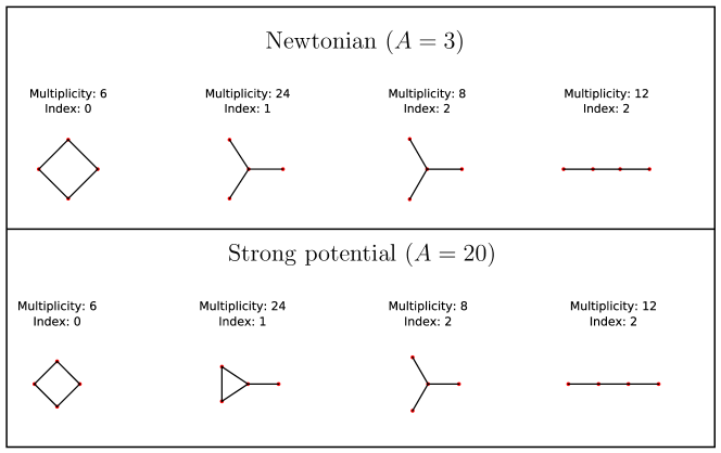
Figure 1. Central configurations of the equal-mass four-body problem for $A=3$ and $A=20$.

For the regular polygon central configuration with $N=4$ (the square), we can compute the radius $r$:

$$r=\left(\frac{2(\sqrt{2})^{2-A}+2^{2-A}}{8}\right)^{\frac{1}{A}}=\left(2^{-1-A}[2^{A/2}+1]\right)^{\frac{1}{A}}$$

(this is a special case of the general result given in Section 2).

We can find the Morse index of the square by explicitly computing the eigenvalues of the Hessian of $f$. The first two of the eight eigenvalues of the Hessian of $f$ are $\lambda_{(4,0,+)}=4A$ and $\lambda_{(4,0,+)}=0$. The other six are more complicated. There are two equal pairs $\lambda_{(4,1,\pm)}=\lambda_{(4,3,\pm)}$, for which

$$P_{1,1}=P_{3,3}=2\left(\frac{2^{A/2}A+2}{1+2^{A/2}}\right)$$

$$Q_{1,1}=Q_{3,3}=\frac{{\left(2^{\frac{1}{2}A+1}A+4\right)}\left({\left(2^{\frac{1}{2}\,A}+2^{A}\right)}2^{-\frac{3}{2}\,A-1}\right)^{\frac{2}{A}}}{1+2^{A/2}}$$

$$S_{1,1}=S_{3,3}=\frac{2(A-2)((2^{A/2}+2^{A})2^{-3A/2-1})^{1/A}}{1+2^{-A/2}}$$

and with these in hand it is not difficult to show that $\lambda_{(4,1,\pm)}=\lambda_{(4,3,\pm)}>0$ for all $A\geq 2$.

Finally $\lambda_{(4,2,\pm)}$ is determined by

$$P_{2,2}=\frac{4A}{1+2^{A/2}}$$

$$Q_{2,2}=\frac{2^{A/2+2}\left({\left(1+2^{A/2}\right)}2^{-A-1}\right)^{\frac{2}{A}}A}{1+2^{A/2}}$$

$$S_{2,2}=0$$

and since the diagonal entries of this block are always positive $\lambda_{(4,2,\pm)}>0$ for all $A\geq 2$.

Thus in the quotient space $\mathcal{C}_{4}$ the eigenvalues are positive and the square is always a minimum of $f$. The same conclusion was reached by Jersett [68] using different methods. Under the direct isometry equivalence relation there are 6 distinct labelings of the square, so it has multiplicity 6.

The equilateral triangle with a mass at its center was also studied in this context by Jersett [68]. It has eigenvalues $0,4,4,4A$ and two pairs of eigenvalues

$$\lambda_{\pm}=\frac{6+3A+(5A-6)3^{A/2}}{3+3^{A/2}}\pm\frac{\sqrt{(16A^{2}+9(A-2)^{2})3^{A}+9(A-2)^{2}(1-2\cdot 3^{A/2})}}{3+3^{A/2}}$$

The pair of eigenvalues $\lambda_{-}$ are negative [68] for all $A\geq 2$, so the Morse index of this configuration is always 2. Any of the four masses can be at the center, and then there are only 2 distinct ways to label the outer triangle (under the orientation-preserving equivalence relation), so the equilateral triangle with a mass at its center has multiplicity 8.

The isosceles central configurations of the four-body problem, which have two pairs of equal mutual distances, are unfortunately much more complicated to analyze. Its lack of rotational symmetry means it has multiplicity 24.

Using the Albouy-Chenciner equations [7, 99] for the isosceles configuration, we excluded most of the mutual distance and $A$-parameter space using interval analysis. After refining the parameter intervals, we then also used a method from [127] to prune interval sets which could not contain a bifurcation (i.e. where the Jacobian of our system must have maximal rank). To summarize this method (Theorem 5 in [127]): for an interval matrix $A$ with entries $[\underline{a},\overline{a}]$, we define the midpoint and radius matrices $mid(A)=(\underline{A}+\overline{A})/2$ and $rad(A)=(\overline{A}-\underline{A})/2$. Then any matrix with entries contained in the interval entries of $A$ has full rank if $\sigma_{max}(rad(A))<\sigma_{min}(mid(A))$, where the $\sigma$ denote the singular values of the singular value decomposition of each matrix; as the inequality on singular values is an exact result, it needs to be strengthened slightly to account for the computational precision.

This interval arithmetic method worked very well for $A>5$, and sufficiently well to exclude bifurcations for $A>3$. However, for $A<3$ it became prohibitively computationally expensive due to the bifurcation at $A=2$ where $f$ is no longer nondegenerate.

Since we know that for $N=4$ the Poincaré polynomial of the configuration space $\mathcal{C}_{4}$ is $P(t)=1+5t+6t^{2}$ [99], the above analysis implies

Theorem 5.

For $A\geq 3$, the Morse polynomial of $f$ is

$$M=P+(1+t)(5+14t)=6+24t+20t^{2}.$$

All of our numerical analysis strongly supports the following conjecture (a slightly stronger version of a speculation in [3]), which we are unable to rigorously prove at this time:

Conjecture 2.

For $A>2$, the Morse polynomial of $f$ is

$$M=P+(1+t)(5+14t)=6+24t+20t^{2}.$$

For our purposes, the case of four equal masses is a somewhat special case in that we believe the Morse indices of the critical points do not change in the interval $(2,\infty)$, although there is a degeneracy for $A=2$. We will see below that for $N>4$ there are bifurcations as $A$ is varied.

3.3. The five-body problem

Much less is known about 5-body central configurations in general compared to $N=4$. In the Newtonian case, the earliest systematic attempt was by Williams [139], who attempted to extend the approach that MacMillan and Bartky [86] pioneered for $N=4$ on convex configurations for general (not necessarily equal) masses; the work of Williams was later improved by Chen and Hsiao [29]. There are limited results on configurations with particular symmetries [56, 81, 57, 51, 83, 32]. Albouy and Kaloshin proved that there are finitely many five-body central configurations in the Newtonian case, apart from some exceptional cases determined by polynomials in the mass parameters for which the result is unknown [10].

For equal masses the central configurations of the five-body problem in the Newtonian case was completely characterized with a homotopy continuation method in [76]. We can use our formula for the eigenvalues of the Hessian of $f$ to compute the Morse index of the regular pentagon. Then using numerical results we speculate on the complete Morse structure of the problem for $A\in[2,\infty)$.

The central configurations for $A=3$, $A=7$, and $A=20$ are shown in Figure 2.

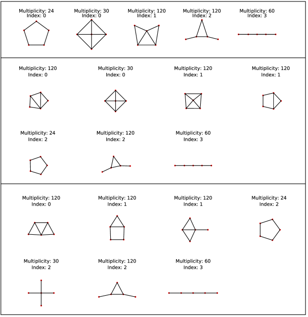
Figure 2. Central configurations of the five-body problem for $A=3$, $A=7$, and $A=20$.

The Hessian of $f$ for the regular pentagon has a bifurcation for some $A\in(6.755,6.756)$. As $A$ increases through this bifurcation value, the regular pentagon goes from having Morse index 0 to Morse index 2, and two new central configurations are created. The first new configuration has index 0, and as $A$ increases its shape becomes close to being three equilateral triangles packed in a row (see Figure 2). The second new configuration has Morse index 1, and its shape approaches a square topped by an equilateral triangle.

An interesting bifurcation occurs at $A\approx 7.5637$. For $A$ below this bifurcation value, there are index-1 central configurations which are symmetric trapezoids with a fifth mass symmetrically placed in the interior of the trapezoid, and the symmetric cross has index 0. At the bifurcation the trapezoid becomes a square, and the symmetric cross becomes degenerate. After the bifurcation (for larger values of $A$) the symmetric cross has index 2, and instead of symmetric trapezoids there are symmetric concave kites with index 1.

We summarize our numerical results by the following conjecture

Conjecture 3.

There are unique values $A_{5}\in(6.755,6.756)$ and $A_{c}\in(7.5636,7.5638)$ such that for $2\leq A<A_{5}$, the Morse polynomial of $f$ on $\mathcal{C}_{5}$ is

$$M(t)=54+120t+120t^{2}+60t^{3}=P(t)+(1+t)(53+58t+36t^{2})$$

for $A_{5}<A<A_{c}$:

$$M(t)=150+240t+144t^{2}+60t^{3}=P(t)+(1+t)(149+82t+36t^{2})$$

and finally for $A_{c}<A$:

$$M(t)=120+240t+174t^{2}+60t^{3}=P(t)+(1+t)(119+112t+36t^{2})$$

(For the 5-body problem the Poincaré polynomial for the reduced configuration space is $P(t)=1+9t+26t^{2}+24t^{3}$.)

3.4. The six-body problem

In Figure 3 we show central configurations of the six-body problem for $A=3$ and $A=20$.

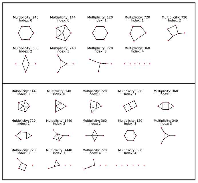
Figure 3. Conjectured central configurations of the six-body problem for $A=3$ and $A=20$.

The Newtonian configuration close in shape to the regular hexagon is a twisted crown; the existence and uniqueness of the relative equilbria with this type of symmetry has been studied in some detail [100, 144, 17].

In the equal-mass case for $A=2$ and $A=3$, it seems from several numerical experiments that the first time a central configuration without any symmetry appears is $N=8$ [14, 47]; in this context it is interesting that as $A$ increases several asymmetric configurations are created from bifurcations already for $N=6$.

Let us consider the asymmetric index-2 central configuration, the seventh in Figure (3), as a case study in what a theory of central configurations for the limit $A\rightarrow\infty$ might look like. Our choice of $f$ was motivated partly by the desire that in the limit $A\rightarrow\infty$, the nearest-neighbor distance would approach $1$. The limiting configuration in question would then be a rhombus composed of equilateral triangles with two masses attached to a single edge. For large $A$, these masses only effectively interact with their single nearest neighbor. Assuming that the core rhombus is robust to small perturbations, we need only determine positions for the single-edge masses so that their single interaction direction is parallel to their position (i.e. pointing towards the center of mass). Denote the rhombus positions by $q_{1},\ldots,q_{4}$, and assume $q_{5}$ only interacts with $q_{1}$, and $q_{6}$ with $q_{2}$, so that $q_{5}=q_{1}+e^{\mathbb{I}\theta_{1}}$ and $q_{6}=q_{2}+e^{\mathbb{I}\theta_{2}}$ . Then (assuming equal masses) the additional constraints on this limit configuration are

$$\sum_{i=1}^{6}q_{i}=0$$

$$\mu_{1}e^{\mathbb{I}\theta_{1}}=q_{5},\ \ \ \mu_{2}e^{\mathbb{I}\theta_{2}}=q_{6}$$

where the $\mu_{i}$ and $\theta_{i}$ are real. This can be converted into a polynomial system with $q_{i}=(x_{i},y_{i})$, which we solved with computer assistance by computing a Gröbner basis using Singular [36] within Sage [137]. Although these equations are much simpler than those of a central configuration for finite $A$, we were somewhat surprised that they require finding roots of sixth-degree polynomials; for example, the position $y_{1}$ is a root of

$$11583+44505y_{1}-9238y_{1}^{2}-71696y_{1}^{3}+52212y_{1}^{4}-21692y_{1}^{5}+7448y_{1}^{6}=0$$

with $y_{1}\approx=1.33$.

For the six-body problem the Poincaré polynomial is $P(t)=1+14t+71t^{2}+154t^{3}+120t^{4}$, and corresponding to Figure (3) we have the following conjectures:

Conjecture 4.

For $6$ bodies, for sufficiently large $A$,

$$M(t)=384+1440t+2520t^{2}+2520t^{3}+1080t^{4}=P(t)+(1+t)(383+1043t+1406t^{2}+960t^{3})$$

and for $A=3$

$$M(t)=384+840t+1080t^{2}+960t^{3}+360t^{4}=P(t)+(1+t)(383+443t+566t^{2}+240t^{3})$$

Support for this comes from the independent investigations of Ferrario [47], who found consistent sets of central configurations in the Newtonian case using a fixed-point method for $N\in\{6,7,8,9\}$.

3.5. The {7, 8, 9}-body problems

For larger $N$, it becomes difficult to find all of the equal mass central configurations for large $A$. For the Newtonian case we have the following conjectures which agree with the numerical results of Ferrario [47] (apart from what may be a typo: the 26th central configuration of the 9-body problem listed by Ferrario should have isotropy 1, rather than the $\frac{1}{2}$ stated there, corresponding to a multiplicity of $9!$ rather than $2\cdot 9!$). In the vortex case ($A=2$) there appear to be exactly 12 central configurations [45], so at least one bifurcations occur between $A=2$ and $A=3$.

Conjecture 5.

The Morse polynomials of $f$ for $A=3$ are

$$\text{for }N=7,\ \ M(t)=120(7+84t+132t^{2}+105t^{3}+84t^{4}+35t^{5})$$

$$\text{for }N=8,\ \ M(t)=720(8+56t+224t^{2}+301t^{3}+210t^{4}+112t^{5}+28t^{6})$$

$$\text{for }N=9,\ \ M(t)=5040(81+216t+384t^{2}+732t^{3}+746t^{4}+396t^{5}+168t^{6}+36t^{7})$$

These conjectured central configurations are pictured in Figures (4), (5), and (6).

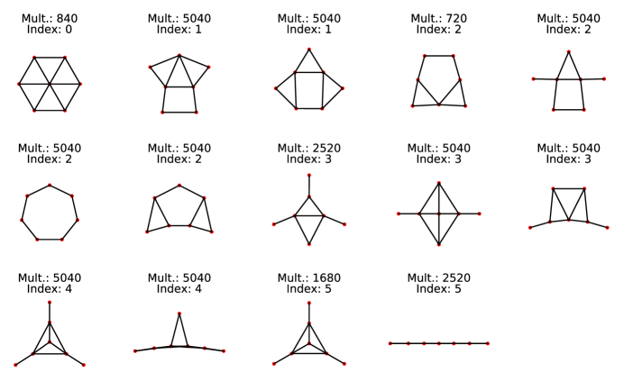
Figure 4. Conjectured central configurations of the equal-mass seven-body problem for $A=3$, with Morse indices and multiplicities.

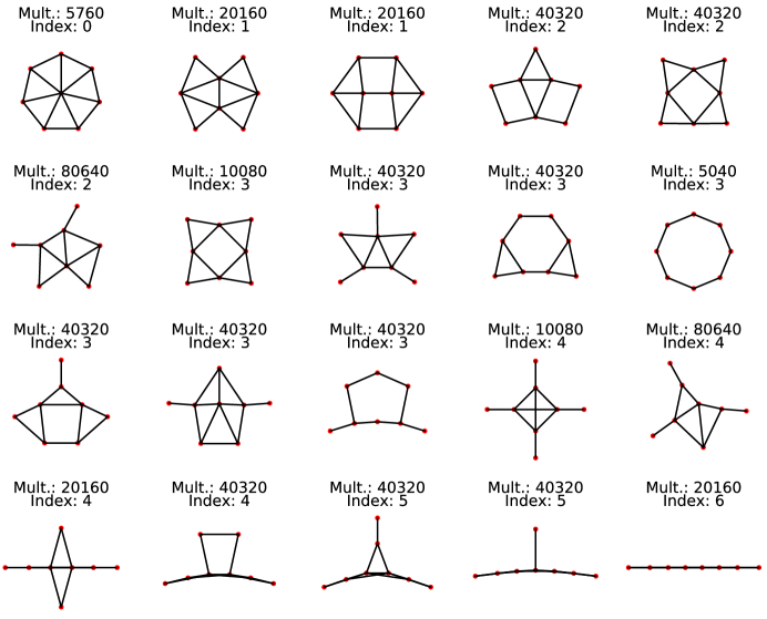
Figure 5. Conjectured central configurations of the equal-mass eight-body problem for $A=3$, with Morse indices and multiplicities.

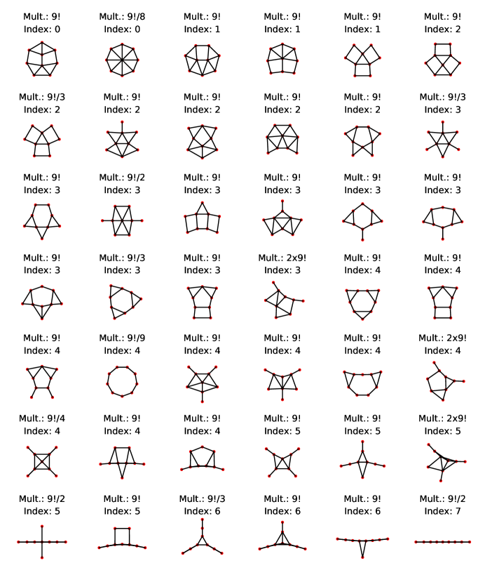
Figure 6. Conjectured central configurations of the equal-mass nine-body problem for $A=3$, with Morse indices and multiplicities.

Our experience so far has also suggested another conjecture:

Conjecture 6.

The number of equal-mass central configurations never decreases as the exponent $A$ increases.

This conjecture may also be true for unequal mass central configurations, but we lack the intuition to be confident in stating this stronger form.

4. Collinear central configurations

Fortunately, results from the Newtonian case on the collinear central configurations can be easily extended to $A\in[2,\infty)$. The following result is something of a folk theorem, I do not know of a reference that explicitly states it:

Theorem 6.

For any $A\in[2,\infty)$, for each ordering of $N$ positive masses on a line there is a unique central configuration, and its (planar) Morse index is $N-2$.

Proof.

The uniqueness of the collinear configurations for a given ordering can be proved as an easy generalization of the argument in [99] (section 2.9 of that work), which shows that the function $f$ is convex on each connected component of the collinear configuration equivalence classes (an elegant proof improving on the original result of Moulton [102]). There is also a proof by Ferrario for homogeneous potentials [47] using a fixed-point method. The statement of the Morse index being $N-2$ can be proved by generalizing the creative argument of C. Conley presented in [105] and [99], as the exponent being $A=3$ plays no essential role in that proof.

∎

The idea of the proof of Conley, which uses an auxiliary dynamical system that converges to collinear configurations, may have inspired a paper of Buck [24] on Newtonian collinear configurations, which would be interesting to generalize to $A\in[2,\infty)$.

5. Future Directions

In addition to the various conjectures given in this article we would like to highlight some more general goals.

1. A similar analysis to the one given here for the regular polygon could be carried out for the $N+1$ problem of a regular polygon with a central mass. If the problem is restricted to all equal masses (i.e. including the central mass), the central mass should become inconsequential for large $N$ and $A$. Much is also already known about nested and ‘twisted’ regular polygon configurations [42, 100, 145, 126, 78, 82, 31, 27, 144, 17, 138, 146] which would be another relatively easy extension.

2. Numerically complete an analysis of all bifurcations in the equal mass $N$-body problem as the potential exponent $A$ is varied in $[2,\infty)$ for $N\in\{6,\ldots,10\}$ (and higher if possible).

3. Find a consistent (within Morse theory) set of central configurations for the equal mass $7$-body problem.

4. Extend any of these results to non-equal masses; even a perturbative analysis near the equal mass case would be a significant advance. It may also be relatively easy to extend to restricted problems (where some of the masses are infinitesimal compared to others), which already have a rich literature of results in the Newtonian case [79, 124, 65, 106, 107, 49, 15, 142, 97, 34, 75, 123, 125, 18, 60].

5. Derive equations, or a combinatorial/linear-algebraic framework, for central configurations in the limiting case of $A\rightarrow\infty$. Compared to the Newtonian case (cf. [23]) it should be much easier to characterize possible central configurations for all $N$. We strongly believe that the development of such a framework is acheivable and will shed useful light on the problem for all $A\geq 2$.

Conflicts of interest

The author declares that he has no conflict of interest.

References

- [1] A. Albouy, Integral manifolds of the -body problem, Invent. math. 114 (1993), 463–488.
- [2] by same author, Symetrie des configurations centrales de quatre corps, C. R. Acad. Sci. Paris Soc. I 320 (1995), no. 2, 217–220.
- [3] by same author, The symmetric central configurations of four equal masses, Hamiltonian dynamics and celestial mechanics, Contemp. Math., vol. 198, Amer. Math. Soc, Providence, RI, 1996, pp. 131–135.
- [4] by same author, On a paper of Moeckel on central configurations, Regular & Chaotic Dynamics. International Scientific Journal 8 (2003), no. 2, 133–142.
- [5] by same author, Open problem 1: Are Palmore’s “ignored estimates” on the number of planar central configurations correct?, Qualitative theory of dynamical systems 14 (2015), no. 2, 403–406.
- [6] A. Albouy, H. E. Cabral, and A. A. Santos, Some problems on the classical n-body problem, Cel. Mech. Dyn. Astron. 113 (2012), no. 4, 369–375.
- [7] A. Albouy and A. Chenciner, Le problème des n corps et les distances mutuelles, Invent. math. 131 (1997), no. 1, 151–184.
- [8] A. Albouy and Y. Fu, Euler configurations and quasi-polynomial systems, Regular and Chaotic Dynamics 12 (2007), 39–55.
- [9] A. Albouy, Y. Fu, and S. Sun, Symmetry of planar four-body convex central configurations, Proceedings of the Royal Society A: Mathematical, Physical and Engineering Sciences 464 (2008), no. 2093, 1355–1365.
- [10] A. Albouy and V. Kaloshin, Finiteness of central configurations of five bodies in the plane, Annals of Math 176 (2012), no. 1, 535–588.
- [11] M. Alvarez-Ramírez and J. Llibre, The symmetric central configurations of the 4-body problem with masses m1= m2 m3= m4, Applied Mathematics and Computation 219 (2013), no. 11, 5996–6001.
- [12] H. Andoyer, Sur l’équilibre relatif de n corps, Bull. Astron. V. 23 (1906), 50–59.
- [13] H. Aref, N. Rott, and H. Thomann, Gröbli’s solution of the three-vortex problem, Annual Review of Fluid Mechanics 24 (1992), no. 1, 1–21.
- [14] H. Aref and D. L. Vainchtein, Point vortices exhibit asymmetric equilibria, Nature 392 (1998), no. 6678, 769.
- [15] R. F. Arenstorff, Central configurations of four bodies with one inferior mass, Cel. Mech. 28 (1982), 9–15.
- [16] V. I. Arnold, The cohomology ring of the colored braid group, Vladimir I. Arnold-Collected Works, Springer, 1969, pp. 183–186.
- [17] E. Barrabés and J. M. Cors, On central configurations of twisted crowns, arXiv:1612.07135.
- [18] J. F. Barros and E. S. G. Leandro, Bifurcations and enumeration of classes of relative equilibria in the planar restricted four-body problem, SIAM J. Math. Anal. 46 (2014), no. 2, 1185–1203.
- [19] A. M. Barry, G. R. Hall, and C. E. Wayne, Relative equilibria of the (1 +n)-vortex problem, J. Nonlinear Science 22 (2012), 63–83.
- [20] V. L. Barutello, R. D. Jadanza, and A. Portaluri, Linear instability of relative equilibria for n-body problems in the plane, J. of Diff. Eq. 257 (2014), no. 6, 1773–1813.
- [21] R. Bott, Morse theory indomitable, Publications Mathématiques de l’Institut des Hautes Études Scientifiques 68 (1988), no. 1, 99–114.
- [22] V. A Brumberg, Permanent configurations in the problem of four bodies and their stability., 1957, pp. 57–79.
- [23] G. Buck, On clustering in central configurations, Proc. Amer. Math. Soc. 108 (1990), no. 3, 801–810.
- [24] by same author, The collinear central configuration of n equal masses, Cel. Mech. Dyn. Astron. 51 (1991), no. 4, 305–317.
- [25] H. E. Cabral, On the integral manifolds of the -body problem, Invent. math. 20 (1973), no. 1, 59–72.
- [26] H. E. Cabral and D. S. Schmidt, Stability of relative equilibria in the problem of vortices, SIAM J. Math. Anal. 31 (1999), no. 2, 231–250.
- [27] M. Celli, E. A. Lacomba, and E. Pérez-Chavela, On polygonal relative equilibria in the n-vortex problem, Journal of Mathematical Physics 52 (2011), no. 10, 103101.
- [28] J. Chazy, Sur certaines trajectoires du problème des n corp, Bull. Astronom. 35 (1918), 321–389.
- [29] K.-C. Chen and J.-S. Hsiao, Strictly convex central configurations of the planar five-body problem, Trans. of the AMS 370 (2018), no. 3, 1907–1924.
- [30] M. Corbera, J. M. Cors, and G. E. Roberts, A four-body convex central configuration with perpendicular diagonals is necessarily a kite, Qualitative Theory of Dynamical Systems (2018), 1–8.
- [31] M. Corbera, J. Delgado, and J. Llibre, On the existence of central configurations of p nested n-gons, Qual. Theory of Dynamical Systems 8 (2009), no. 2, 255–265.
- [32] J. L. Cornelio, M. Álvarez-Ramírez, and J. M. Cors, A family of stacked central configurations in the planar five-body problem, Celestial Mechanics and Dynamical Astronomy 129 (2017), no. 3, 321–328.
- [33] J. M. Cors, G. R. Hall, and G. E. Roberts, Uniqueness results for co-circular central configurations for power-law potentials, Physica D: Nonlinear Phenomena 280 (2014), 44–47.
- [34] J. M. Cors, J. Llibre, and M. Ollé, Central configurations of the planar coorbital satellite problem, Cel. Mech. and Dyn. Astron. 89 (2004), no. 4, 319.
- [35] J. M. Cors and G. E. Roberts, Four-body co-circular central configurations, Nonlinearity 25 (2012), no. 2, 343.
- [36] W. Decker, G.-M. Greuel, G. Pfister, and H. Schönemann, Singular 4-1-0 — a computer algebra system for polynomial computations, 2016, http://www.singular.uni-kl.de.
- [37] Yiyang Deng, Bingyu Li, and Shiqing Zhang, Four-body central configurations with adjacent equal masses, Journal of Geometry and Physics 114 (2017), 329–335.
- [38] R. L. Devaney, Triple collision in the planar isosceles three body problem, Invent. math. 60 (1980), no. 3, 249–267.
- [39] O. Dziobek, Über einen merkwürdigen Fall des Vielkörperproblem, Astron. Nachr. 152 (1900), 33–46.
- [40] R. Easton, Some topology of -body problems, J. Diff. Eq. 19 (1975), 258–269.
- [41] M. S. ElBialy, Collision singularities in celestial mechanics, SIAM J. Math. Anal. 21 (1990), no. 6, 1563–1593.
- [42] B. Elmabsout, Nouvelles configurations d’équilibre relatif dans le problème des n corps. I, Comptes rendus de l’Académie des sciences. Série 2, Mécanique, Physique, Chimie, Sciences de l’univers, Sciences de la Terre 312 (1991), no. 5, 467–472.
- [43] B. Érdi and Z. Czirják, Central configurations of four bodies with an axis of symmetry, Cel. Mech. Dyn. Astron. 125 (2016), no. 1, 33–70.
- [44] L. Euler, De motu rectilineo trium corporum se mutuo attrahentium, Novi Comm. Acad. Sci. Imp. Petrop 11 (1767), 144–151.
- [45] J.-C. Faugère and J. Svartz, Solving polynomial systems globally invariant under an action of the symmetric group and application to the equilibria of n vortices in the plane, Proceedings of the 37th International Symposium on Symbolic and Algebraic Computation, ACM, 2012, pp. 170–178.
- [46] A. C. Fernandes, J. Llibre, and L. F. Mello, Convex central configurations of the 4-body problem with two pairs of equal adjacent masses, Archive for Rational Mechanics and Analysis 226 (2017), no. 1, 303–320.
- [47] D. L. Ferrario, Central configurations, symmetries and fixed points, arXiv preprint math/0204198 (2002), 1–47.
- [48] by same author, Central configurations and mutual differences, SIGMA. Symmetry, Integrability and Geometry: Methods and Applications 13 (2017), 021.
- [49] J. R. Gannaway, Determination of all central configurations in the planar four-body problem with one inferior mass, Ph.D. thesis, Vanderbilt University, TN, 1981.
- [50] M. Gascheau, Examen d’une classe d’équations différentielles et application à un cas particulier du probl’éme des trois corps, Compt. Rend. 16 (1843), 393–394.
- [51] M. Gidea and J. Llibre, Symmetric planar central configurations of five bodies: Euler plus two, Cel. Mech. and Dyn. Astron. 106 (2010), no. 1, 89.
- [52] J. Hachmeister, J. Little, J. McGhee, R. Pelayo, and S. Sasarita, Continua of central configurations with a negative mass in the -body problem, Cel. Mech. Dyn. Astron. 115 (2013), 427–438.
- [53] G. R. Hall, Central configurations in the planar 1+ body problem, preprint, Boston University, 1988.
- [54] M. Hampton, Concave central configurations in the four-body problem, Ph.D. thesis, University of Washington, Seattle, WA, 2002.
- [55] by same author, Co-circular central configurations in the four-body problem, EQUADIFF 2003, World Sci. Publ., Hackensack, NJ, 2005, pp. 993–998.
- [56] by same author, Stacked central configurations: new examples in the planar five-body problem, Nonlinearity 18 (2005), no. 5, 2299–2304.
- [57] by same author, Finiteness of kite relative equilibria in the Five-Vortex and Five-Body problems, Qualitative Theory of Dynamical Systems 8 (2010), no. 2, 349–356.
- [58] by same author, Splendid isolation: local uniqueness of the centered co-circular relative equilibria in the n-body problem, Cel. Mech. Dyn. Astron. 124 (2016), 145–153.
- [59] M. Hampton and A. N. Jensen, Finiteness of spatial central configurations in the five-body problem, Cel. Mech. Dyn. Astron. 109 (2011), no. 4, 321–332.
- [60] by same author, Finiteness of relative equilibria in the planar generalized -body problem with fixed subconfigurations, J. Geom. Mech. 7 (2015), 35–42.
- [61] M. Hampton and R. Moeckel, Finiteness of relative equilibria of the four-body problem, Invent. math. 163 (2005), no. 2, 289–312.
- [62] by same author, Finiteness of stationary configurations of the four-vortex problem, Trans. of the AMS 361 (2009), no. 3, 1317–1332.
- [63] M. Hampton, G. E. Roberts, and M. Santoprete, Relative equilibria in the four-body problem with two pairs of equal vorticities, J. Nonlinear Sci. 24 (2014), 39–92.
- [64] H. Helmholtz, Uber integrale der hydrodynamischen gleichungen, welche den wirbelbewegungen entsprechen, Crelle’s Journal für Mathematik 55 (1858), 25–55, English translation by P. G. Tait, P.G., On the integrals of the hydrodynamical equations which express vortex-motion, Philosophical Magazine, (1867) 485-51.
- [65] C. Holtom, Permanent configurations in the n-Body problem, Trans. Amer. Math. Soc. 54 (1943), no. 3, 520–543.
- [66] X. Hu and S. Sun, Stability of relative equilibria and Morse index of central configurations, C. R. Acad. Sci. Paris 347 (2009), 1309–1312.
- [67] N. Hulkower, The zero energy three body problem, Indiana University Mathematics Journal 27 (1978), 409–447.
- [68] N. J. Jersett, Planar central configurations of the 4-body problem, Master’s thesis, University of Minnesota Duluth, 2018.
- [69] G. Kirchhoff, Vorlesungen über mathematische physik, B.G. Teubner, 1883.
- [70] E. A. Lacomba, Singularities and chaos in classical and celestial mechanics, Developments in Mathematical and Experimental Physics, Springer, 2003, pp. 89–97.
- [71] E. A. Lacomba and L. A. Ibort, Origin and infinity manifolds for mechanical systems with homogeneous potentials, Acta Applicandae Mathematica 11 (1988), no. 3, 259–284.
- [72] J. L. Lagrange, Essai sur le problème des trois corps, Œuvres, vol. 6, Gauthier-Villars, Paris, 1772.
- [73] E. Laura, Sulle equazioni differenziali canoniche del moto di un sistema di vortici elementari rettilinei e paralleli in un fluido incomprensibile indefinito, Atti della Reale Accad. Torino 40 (1905), 296–312.
- [74] E. S. G. Leandro, Finiteness and bifurcations of some symmetrical classes of central configurations, Arch. Rat. Mech. Anal. 167 (2003), no. 2, 147–177.
- [75] by same author, On the central configurations of the planar restricted four-body problem, J. Diff. Eq. 226 (2006), no. 1, 323–351.
- [76] T. L. Lee and M. Santoprete, Central configurations of the five-body problem with equal masses, Cel. Mech. and Dynam. Astron. 104 (2009), 369–381.
- [77] R. Lehmann-Filhés, Ueber zwei Fälle des Vielkörperproblems., Astron. Nachr. 127 (1891), no. 9, 137–143.
- [78] J. Lei and M. Santoprete, Rosette central configurations, degenerate central configurations and bifurcations, Cel. Mech. Dyn. Astron. 94 (2006), no. 3, 271–287.
- [79] M. Lindlow, Ein Spezialfall des Vierkörperproblems, Astron. Nachr. 216 (1922), 233–248.
- [80] J. Llibre, On the number of central configurations in the n-body problem, Cel. Mech. Dyn. Astron. 50 (1990), no. 1, 89–96.
- [81] J. Llibre and L. F. Mello, New central configurations for the planar 5-body problem, Cel. Mech. Dynam. Astron. 100 (2008), no. 2, 141–149.
- [82] by same author, Triple and quadruple nested central configurations for the planar n-body problem, Physica D: Nonlinear Phenomena 238 (2009), no. 5, 563–571.
- [83] J. Llibre, L. F. Mello, and E. Perez-Chavela, New stacked central configurations for the planar 5-body problem, Celestial Mechanics and Dynamical Astronomy 110 (2011), no. 1, 43.
- [84] Y. Long and S. Sun, Four-body central configurations with some equal masses, Arch. Rat. Mech. Anal. 162 (2002), no. 1, 25–44.
- [85] W. R. Longley, Some particular solutions in the problem of n-bodies, Bull. Am. Math. Soc. 7 (1907), 324–335.
- [86] W. D. MacMillan and W. Bartky, Permanent configurations in the problem of four bodies, Trans. Amer. Math. Soc. 34 (1932), 838–875.
- [87] C. K. McCord, Planar central configuration estimates in the n-body problem, Ergodic Theory and Dynamical Systems 16 (1996), no. 5, 1059–1070.
- [88] C. K. McCord, K. R. Meyer, and Q. Wang, The integral manifolds of the three body problem, vol. 628, American Mathematical Society, 1998.
- [89] R. McGehee, Triple collision in the collinear three-body problem, Invent. math. 27 (1974), no. 3, 191–227.
- [90] J. C. Merkel, Morse theory and central configurations in the spatial n-body problem, J. of Dyn. and Diff. Eq. 20 (2008), no. 3, 653–668.
- [91] K. R. Meyer and D. S. Schmidt, Bifurcations of relative equilibria in the N-body and Kirchhoff problems, SIAM J. Math. Anal. 19 (1988), no. 6, 1295–1313.
- [92] J. Milnor, Morse theory, vol. 51, Princeton University press, 2016.
- [93] R. Moeckel, Orbits of the three-body problem which pass infinitely close to triple collision, American Journal of Mathematics 103 (1981), no. 6, 1323–1341.
- [94] by same author, Chaotic dynamics near triple collision, Arch. Rat. Mech. Anal. 107 (1989), no. 1, 37–69.
- [95] by same author, On central configurations, Mathematische Zeitschrift 205 (1990), no. 1, 499–517.
- [96] by same author, Linear stability of relative equilibria with a dominant mass, J. Dyn. and Diff. Eq. 6 (1994), 37–51.
- [97] by same author, Relative equilibria with clusters of small masses, J. Dyn. Diff. Eq. 9 (1997), 507–533.
- [98] by same author, Generic finiteness for Dziobek configurations, Trans. Amer. Math. Soc. 353 (2001), no. 11, 4673–4686.
- [99] by same author, Central Configurations, Central Configurations, Periodic Orbits, and Hamiltonian Systems, Springer, 2015.
- [100] R. Moeckel and C. Simó, Bifurcation of spatial central configurations from planar ones, SIAM J. Math. Anal. 26 (1995), no. 4, 978–998.
- [101] J. Montaldi, Existence of symmetric central configurations, Cel. Mech. Dyn. Astr. 122 (2015), 405–418.
- [102] F. R. Moulton, The straight line solutions of the problem of N bodies, The Annals of Mathematics 12 (1910), no. 1, 1–17.
- [103] I. Newton, Philosophiæ naturalis principia mathematica, Royal Society, London, 1687.
- [104] K. A. O’Neil, Stationary configurations of point vortices, Trans. of the AMS 302 (1987), no. 2, 383–425.
- [105] F. Pacella, Central configurations of the n-body problem via the equivariant Morse theory, Arch. Rat. Mech. Anal. 97 (1987), 59–74.
- [106] P. Pedersen, Librationspunkte im restringierten vierkoerperproblem, Publikationer og mindre Meddeler fra Kobenhavns Observatorium 137 (1944), 1–80.
- [107] by same author, Stabilitätsuntersuchungen im restringierten vierkörperproblem, Publikationer og mindre Meddeler fra Kobenhavns Observatorium 159 (1952), 1–38.
- [108] E. Perez-Chavela and M. Santoprete, Convex four-body central configurations with some equal masses, Archive for rational mechanics and analysis 185 (2007), no. 3, 481–494.
- [109] L. M. Perko and E. L. Walter, Regular polygon solutions of the n-body problem, Proc. Amer. Math. Soc. 94 (1985), 301–309.
- [110] E. Piña and P. Lonngi, Central configurations for the planar Newtonian four-body problem, Cel. Mech. Dyn. Astron. 108 (2010), no. 1, 73–93.
- [111] A. S. Rayl, Stability of permanent configurations in the problem of four bodies, Ph.D. thesis, University of Chicago, Chicago, IL, 1939.
- [112] G. E. Roberts, A continuum of relative equilibria in the five-body problem, Physica D: Nonlinear Phenomena 127 (1999), no. 3-4, 141–145.
- [113] by same author, Spectral instability of relative equilibria in the planar -body problem, Nonlinearity 12 (1999), no. 4, 757–769.
- [114] by same author, Linear stability in the -gon relative equilibrium, Hamiltonian systems and celestial mechanics (Pátzcuaro, 1998), World Sci. Monogr. Ser. Math., vol. 6, World Sci. Publ., River Edge, NJ, 2000, pp. 303–330.
- [115] by same author, Linear stability of the elliptic Lagrangian triangle solutions in the three-body problem, J. of Diff. Eq. 182 (2002), 191–218.
- [116] by same author, Stability of relative equilibria in the planar -vortex problem, SIAM J. Applied Dynamical Systems 12 (2013), 1114–1134.
- [117] E. J. Routh, On Laplace’s three particles with a supplement on the stability of their motion, Proc. London Math. Soc. 6 (1875), 86–97.
- [118] D. Rusu and M. Santoprete, Bifurcations of central configurations in the four-body problem with some equal masses, SIAM Journal on Applied Dynamical Systems 15 (2016), no. 1, 440–458.
- [119] D. G. Saari, On the role and properties of -body central configurations, Cel. Mech. 21 (1980), 9–20.
- [120] by same author, Collisions, rings, and other Newtonian -body problems, American Mathematical Society, 2005.
- [121] M. Santoprete, Linear stability of the Lagrangian triangle solutions for quasihomogeneous potentials, Cel. Mech. and Dyn. Astron. 94 (2006), 17–35.
- [122] by same author, Four-body central configurations with one pair of opposite sides parallel, Journal of Mathematical Analysis and Applications 464 (2018), no. 1, 421–434.
- [123] A. A. Santos and C. Vidal, Symmetry of the restricted 4+ 1 body problem with equal masses, Regular and Chaotic Dynamics 12 (2007), no. 1, 27–38.
- [124] W. Schaub, Über einen speziellen fall des fünfkörperproblems, Astronomische Nachrichten 236 (1929), no. 3-4, 33–54.
- [125] D. J. Scheeres and N. X. Vinh, Linear stability of a self-gravitating ring, Cel. Mech. Dyn. Astron. 51 (1991), no. 1, 83–103.
- [126] M. Sekiguchi, Bifurcation of central configuration in the 2n+ 1 body problem, Cel. Mech. Dyn. Astron. 90 (2004), no. 3-4, 355–360.
- [127] S. P. Shary, On full-rank interval matrices, Numerical Analysis and Applications 7 (2014), 241–254.
- [128] J. Shi and Z. Xie, Classification of four-body central configurations with three equal masses, Journal of Mathematical Analysis and Applications 363 (2010), no. 2, 512–524.
- [129] M. Shub, Appendix to Smale’s paper: Diagonals and relative equilibria, Manifolds—Amsterdam 1970, Springer, 1971, pp. 199–201.
- [130] C. Simo, Relative equilibrium solutions in the four body problem, Cel. Mech. Dyn. Astron. 18 (1978), no. 2, 165–184.
- [131] E. E. Slaminka and K. D. Woerner, Central configurations and a theorem of Palmore, Cel. Mech. Dyn. Astron. 48 (1990), no. 4, 347–355.
- [132] S. Smale, Topology and mechanics. i, Invent. math. 10 (1970), no. 4, 305–331.
- [133] by same author, Topology and mechanics. II, Invent. math. 11 (1970), no. 1, 45–64.
- [134] by same author, Mathematical problems for the next century, Mathematical Intelligencer 20 (1998), 7–15.
- [135] W. L. Sweatman, Orbits near central configurations for four equal masses, Cel. Mech. Dyn. Astron. 119 (2014), no. 3-4, 379–395.
- [136] J. L. Synge, The apsides of general dynamical systems, Trans. of the AMS 34 (1932), no. 3, 481–522.
- [137] The Sage Developers, Sagemath, the Sage Mathematics Software System (Version 8.3), 2018, http://www.sagemath.org.
- [138] Z. Wang and F. Li, A note on the two nested regular polygonal central configurations, Proc. of the AMS 143 (2015), no. 11, 4817–4822.
- [139] W. L. Williams, Permanent configurations in the problem of five bodies, Trans. of the AMS 44 (1938), no. 3, 563–579.
- [140] A. Wintner, The analytical foundations of celestial mechanics, Princeton University Press, Princeton, NJ, 1941.
- [141] K. D. Woerner, The -gon is not a local minimum of for , Cel. Mech. Dyn. Astron. 49 (1990), no. 4, 413–421.
- [142] Z. Xia, Central configurations with many small masses, J. Diff. Eq. 91 (1991), 168–179.
- [143] Z. Xie, Isosceles trapezoid central configurations of the Newtonian four-body problem, Proceedings of the Royal Society of Edinburgh Section A: Mathematics 142 (2012), no. 3, 665–672.
- [144] X. Yu and S. Zhang, Twisted angles for central configurations formed by two twisted regular polygons, J. of Diff. Eq. 253 (2012), no. 7, 2106–2122.
- [145] S. Zhang and Q. Zhou, Nested regular polygon solutions for planar -body problems, Science in China Series A: Mathematics 45 (2002), no. 8, 1053–1058.
- [146] F. Zhao and J. Chen, Central configurations for -body problems, Cel. Mech. Dyn. Astron. 121 (2015), no. 1, 101–106.