An Online-Learning Approach to Inverse Optimization

Abstract

In this paper, we demonstrate how to learn the objective function of a decision-maker while only observing the problem input data and the decision-maker’s corresponding decisions over multiple rounds. We present exact algorithms for this online version of inverse optimization which converge at a rate of $\mathcal{O}(1/\sqrt{T})$ in the number of observations $T$ and compare their further properties. Especially, they all allow taking decisions which are essentially as good as those of the observed decision-maker already after relatively few iterations, but are suited best for different settings each. Our approach is based on online learning and works for linear objectives over arbitrary feasible sets for which we have a linear optimization oracle. As such, it generalizes previous approaches based on KKT-system decomposition and dualization. We also introduce several generalizations, such as the approximate learning of non-linear objective functions, dynamically changing as well as parameterized objectives and the case of suboptimal observed decisions. When applied to the stochastic offline case, our algorithms are able to give guarantees on the quality of the learned objectives in expectation. Finally, we show the effectiveness and possible applications of our methods in indicative computational experiments.

Keywords: Learning Objective Functions, Online Learning, Inverse Optimization, Multiplicative Weights Update Algorithm, Online Gradient Descent, Mixed-Integer Programming

Mathematics Subject Classification: 68Q32 - 68T05 - 90C59 - 90C11

1 Introduction

Human decision-makers are very good at taking decisions under rather imprecise specification of the decision-making problem, both in terms of constraints as well as objective. One might argue that the human decision-maker can pretty reliably learn from observed previous decisions – a traditional learning-by-example setup. At the same time, when we try to turn these decision-making problems into actual optimization problems, we often run into all types of issues in terms of specifying the model. In an optimal world, we would be able to infer or learn the optimization problem from previously observed decisions taken by an expert.

This problem naturally occurs in many settings where we do not have direct access to the decision-maker’s preference or objective function but can observe the resulting behaviour, and where the learner as well as the decision-maker have access to the same information. Natural examples are as diverse as making recommendations based on user history and strategic planning problems, where the agent’s preferences are unknown but the system is observable. Other examples include knowledge transfer from a human planner into a decision support system: often human operators have arrived at finely-tuned “objective functions” through many years of experience, and in many cases it is desirable to replicate the decision-making process both for scaling up and also for potentially including it in large-scale scenario analysis and simulation to explore responses under varying conditions.

Here, we consider the learning of preferences or objectives from an expert by means of observing the actions taken. More precisely, we observe a set of input parameters and corresponding decisions of the form $\{(p_{1},x_{1}),\dots,(p_{T},x_{T})\}$. They are such that $p_{t}\in P$ with $t=1,\ldots,T$ is a certain realization of problem parameters from a given set $P\subseteq\mathbbm{R}^{k}$. Furthermore, $x_{t}$ is an optimal solution to the optimization problem

$$\max\{c_{\text{true}}^{\top}x\mid x\in X(p_{t})\},$$

where $c_{\text{true}}\in\mathbbm{R}^{n}$ is the expert’s true but unknown objective and $X(p_{t})\subseteq\mathbbm{R}^{n}$ for some (fixed) $n$. We assume that we have full information on the feasible set $X(p_{t})$ and that we can compute $\operatorname{argmax}{\{c^{\top}x\mid x\in X(p_{t})\}}$ for any candidate objective $c\in\mathbbm{R}^{n}$ and $t=1,\dots,T$. We present an online-learning framework that allows us to learn a strategy $(c_{1},\ldots,c_{T})$ of subsequent objective function choices with the following guarantee: if we optimize according to the surrogate objective function $c_{t}$ instead of the actual unknown objective function $c_{\text{true}}$ in response to parameter realization $p_{t}$, we obtain a sequence of optimal decisions (w.r.t. to each $c_{t}$) given by

$$\bar{x}_{t}=\operatorname{argmax}{\{c_{t}^{\top}x\mid x\in X(p_{t})\}}$$

that are essentially as good as the decisions $x_{t}$ taken by the expert on average. To this end, we interpret the observations of parameters and expert solutions as revealed over multiple rounds such that in each round $t$ we are shown the parameters $p_{t}$ first, then take our optimal decision $\bar{x}_{t}$ according to our objective function $c_{t}$, afterwards we are shown the solution $x_{t}$ chosen by the expert, and finally we are allowed to update $c_{t}$ for the next round. For this setup, we will be able to show that our online-learning algorithms are able to produce a strategy of objective functions and corresponding solutions for which both the deviations in true cost $c_{\text{true}}^{\top}(x_{t}-\bar{x}_{t})\geq 0$ as well as the deviations in surrogate cost $c_{t}^{\top}(\bar{x}_{t}-x_{t})\geq 0$ can be made arbitrarily small on average under very general assumptions. This way, our approach can be understood as an online, multi-sample version of inverse optimization, where the typical task is to find an objective function which is close to a known target obective and makes a given solution optimal.

Our results show that linear objective functions over general feasible sets can be learned from relatively few observations of historical optimal parameter-solution pairs. We will derive various extensions of our scheme, such as approximately learning non-linear objective functions and learning from suboptimal decisions. We will also, briefly, discuss the case where the objective $c_{\text{true}}$ is known, but some linear constraints are unknown in this paper.

Literature Overview

The idea of learning or inferring parts of an optimization model from data is a reasonably well-studied problem under many different assumptions and applications and has gained significant attention in the optimization community over the last few years, as discussed for example in den Hertog and Postek, (2016), Lodi, (2016) or Simchi-Levi, (2014). These works argue that there would be significant benefits in combining traditional optimization models with data-derived components. Most approaches in the literature focus on deriving the objective function of an expert decision-maker in a static fashion, based on past observations of input data and the decisions he took in each instance. In almost all cases, the objective functions are learned by considering the KKT-conditions or the dual of the (parameterized) optimization problem, and as such convexity for both the feasible region and the objective function is inherently assumed; examples include Keshavarz et al., (2011); Li, (2016); Thai and Bayen, (2018). Especially, in Esfahani et al., (2018); Troutt et al., (2005, 2006) the authors study the minimization of the same regret function that we consider in the present paper. However, as their exact solution approaches are based on duality, they do not extend to the integer case like the ideas presented here. Sometimes also distributional assumptions regarding the observations are made. In Troutt et al., (2011), the authors study experimental setups for learning objectives under various stochastic assumptions, focussing on maximum likelihood estimation, which is generally the case for their line of work; we make no such assumptions. Especially, the observations can be chosen by a fully-adaptive adversary in our framework.

Closely related to learning optimization models from observed data is the subject of inverse optimization. Here the goal is to find an objective function that renders the observed solutions optimal with respect to the concurrently observed parameter realizations. Approaches in this field mostly stem from convex optimization, and they are used for inverse optimal control (Iyengar and Kang, (2005); Panchea and Ramdani, (2015); Molloy et al., (2016)), inverse combinatorial optimization (D. Burton, (1997); Burton and Toint, (1994, 1992); Sokkalingam et al., (1999); Ahuja and Orlin, (2000)), integer inverse optimization (Schaefer, (2009)) and inverse optimization in the presence of noisy data, such as observed decisions that were suboptimal (Aswani et al., (2018); Chan et al., (2019)). In this paper, we actually do inverse optimization by means of online-learning algorithms.

We remark that our work is also related to inverse reinforcement learning and apprenticeship learning, where the reward function is the target to be learned. However, in this case the underlying problem is modelled as a Markov decision process (MDP); see, for example, the results in Syed and Schapire, (2007) and Ratia et al., (2012). Typically, the obtained guarantees are therefore of a different form.

Applications of such approaches are as diverse as energy systems (Ratliff et al., (2014); Konstantakopoulos et al., (2016)), robot motion (Papadopoulos et al., (2016); Yang et al., (2014)), medicine (Sayre and Ruan, (2014)) and revenue management (Kallus and Udell, (2015); Qiang and Bayati, (2016); Chen et al., (2015); Kallus and Udell, (2016); Bertsimas and Kallus, (2016)); including situations where the observed decisions were not necessarily optimal (Nielsen and Jensen, (2004)).

Contribution

To the best of the authors’ knowledge, this is the first attempt to learn the objective function of an optimization model from data using an online-learning approach. All previous approaches heavily rely on duality and thus require convexity assumptions both for the feasible region as well as the objectives. As such, they cannot deal with more complex, possibly non-convex decision domains. This in particular includes the important case of integer-valued decisions (such as yes/no-decisions or, more generally, mixed-integer programming) and also many other non-convex setups (several of which admit efficient linear optimization algorithms). Previously, this was only possible when the structure of the feasible set could be beneficially exploited. In contrast, our approach does not make any such assumptions and only requires access to a linear optimization oracle (in short: LP oracle) for the feasible region $X$. Such an oracle is defined as a method which, given a vector $c\in\mathbbm{R}^{n}$, returns $\operatorname{argmax}{\{c^{\top}x\mid x\in X\}}$. Thus, we do not explicitly analyse the KKT-system or the dual program (in the case of linear programs (LPs); see Remark 3.2). Actually, one might consider our approach as an algorithmic analogue of the KKT-system (or dual program) in the convex case.

Classical inverse optimization only treats the offline case, where all observations are present in advance. Our new approach is based on online learning algorithms, especially the Multiplicative Weights Update (MWU) algorithm developed in Littlestone and Warmuth, (1994), Vovk, (1990) as well as Freund and Schapire, (1997) (see Arora et al., (2012); Hazan, (2016) for a comprehensive introduction; see also Audibert et al., (2013)). A similar algorithm was used in Plotkin et al., (1995) for solving fractional packing and covering problems. To generalize the applicability of our approach, we also derive a second algorithm based on Online Gradient Descent (OGD) due to Zinkevich (see Zinkevich, (2003)) and study approaches based on follow-the-leader schemes (see Hazan, (2016) for an introduction). We remark that our approaches are equivalent to Mirror Descent Nemirovski, (1979) for suitable domains and loss function, however, the interpretation here is different. We finally point out that our feedback is stronger than bandit feedback. This requirement is not unexpected as the costs chosen by the “adversary” depend on our decision; as such the bandit model (see, for example, Dani et al., (2008); Abbasi-Yadkori et al., (2011)) does not readily apply.

In an indicative set of computational experiments, we demonstrate the effectiveness and wide applicability of our algorithmic approach. To this end, we investigate its use for learning the objective functions of several combinatorial optimization problems that are relevant in practice and are able to show, among other things, that the learned objective generalizes to previously unseen data samples very well.

The present paper is the full version of a contribution to the International Conference on Machine Learning (ICML) 2017, see Bärmann et al., (2017). The follow-up works Ward et al., (2019) and Dong et al., (2018) by different authors which have been published in the meantime study a specialization of our approach to projective cone scheduling and implicit update rules respectively. The authors of Sessa et al., (2020) treat robust optimization under an uncertain objective function where a bandit approach adjusts the level of conservativeness. In the appendix, we give further analyses on the results presented here.

2 Problem Setting

We consider the following family of optimization problems $(\textrm{OPT}(p))_{p}$, which depend on parameters $p\in P\subseteq\mathbbm{R}^{k}$ for some $k\in\mathbbm{N}$:

$$\max\{c_{\text{true}}^{\top}x\mid x\in X(p)\},$$

where $c_{\text{true}}\in\mathbbm{R}^{n}$ is the objective function and $X(p)\subseteq\mathbbm{R}^{n}$ is the feasible region, which depends on the parameters $p$. Of particular interest to us will be feasible regions that arise as polyhedra defined by linear constraints and their intersections with integer lattices, i.e. the cases of LPs and MIPs:

$$X(p)=\{x\in\mathbbm{Z}^{n-l}\times\mathbbm{R}^{l}\mid A(p)x\leq b(p)\}$$

with $A(p)\in\mathbbm{R}^{m\times n}$ and $b(p)\in\mathbbm{R}^{m}$. However, our approach can also readily be applied in the case of more complex feasible regions, such as mixed-integer sets bounded by a convex function $G\colon P\times\mathbbm{Z}^{n-l}\times\mathbbm{R}^{l}\to\mathbbm{R}$:

$$X(p)=\{x\in\mathbbm{Z}^{n-l}\times\mathbbm{R}^{l}\mid G(p,x)\leq 0\},$$

or even more general settings. In fact, for any possible choice of model for the sets of feasible decisions, we only require the availability of a linear optimization oracle, i.e. an algorithm which is able to determine $\operatorname{argmax}{\{c^{\top}x\mid x\in X(p)\}}$ for any $c\in\mathbbm{R}^{n}$ and $p\in P$. We call a decision $x\in\mathbbm{R}^{n}$ optimal for $p$ if it is an optimal solution to $\textrm{OPT}(p)$.

We assume that Problem $\textrm{OPT}(p)$ models a parameterized optimization problem which has to be solved repeatedly for various input parameter realizations $p$. Our task is to learn the fixed objective function $c_{\text{true}}$ from given observations of the parameters $p$ and a corresponding optimal solution $x$ to $\textrm{OPT}(p)$. To this end, we further assume that we are given a series of observations $((p_{t},x_{t}))_{t}$ of parameter realizations $p_{t}\in P$ together with an optimal solution $x_{t}$ to $\textrm{OPT}(p_{t})$ computed by the expert for $t=1,\ldots,T$; these observations are revealed over time in an online fashion: in round $t$, we obtain a parameter setting $p_{t}$ and compute an optimal solution $\bar{x}_{t}\in X(p_{t})$ with respect to an objective function $c_{t}$ based on what we have learned about $c_{\text{true}}$ so far. Then we are shown the solution $x_{t}$ the expert with knowledge of $c_{\text{true}}$ would have taken and can use this information to update our inferred objective function for the next round. In the end, we would like to be able to use our inferred objective function to take decisions that are essentially as good as those chosen by the expert in an appropriate aggregation measure such as, for example, “on average” or “with high probability”. The quality of the inferred objective is measured in terms of cost deviation between our solutions $\bar{x}_{t}$ and the solutions $x_{t}$ obtained by the expert – details of which will be given in the next section.

To fix some useful notations, let $v(i)$ denote the $i$-th component of a vector $v$ throughout, and let $[n]\coloneqq\{1,\dots,n\}$ for any natural number $n$. Furthermore, let $\mathbbm{1}^{n}\coloneqq(1,\ldots,1)^{\top}$ denote the all-ones vector in $\mathbbm{R}^{n}$. Finally, we need a suitable measure for the diameter of a given set.

Definition 2.1.

The $\ell_{p}$-diameter of a set $S\subseteq\mathbbm{R}^{n}$, denoted by $\operatorname{diam}_{p}(S)$, is the largest distance between any two points $x_{1},x_{2}\in S$, measured in the $p$-norm, $1\leq p\leq\infty$, i.e. $\operatorname{diam}_{p}(S)\coloneqq\max_{x_{1},x_{2}\in S}\lVert x_{1}-x_{2}\rVert_{p}$.

As a technical assumption, we further demand that $c_{\text{true}}\in F$ for some convex, compact and non-empty subset $F\subseteq\mathbbm{R}^{n}$ which is known beforehand. This is no actual restriction, as $F$ could be chosen to be any ball according to some $p$-norm, $1\leq p\leq\infty$, for example. In particular, this ensures that we do not have to deal with issues that arise when rescaling our objective.

3 Learning Objectives

One approach to find a candidate for the true objective function $c_{\text{true}}$ is to solve the following optimization problem:

$$\min_{c\in F}\sum_{t\in[T]}\left(\left(\max_{x\in X(p_{t})}c^{\top}x\right)-c^{\top}x_{t}\right),$$ (1)

where $\lVert\cdot\rVert\colon\mathbbm{R}^{n}\to\mathbbm{R}_{+}$ is an arbitrary norm on $\mathbbm{R}^{n}$ and $x_{t}\in X(p)$ is the optimal decision taken by the expert in round $t$. The true objective function $c_{\text{true}}$ is an optimal solution to Problem (1) with objective value $0$. This is because any solution $\hat{c}\in F$ is feasible and produces non-negative summands $\left(\max_{x\in X(p_{t})}\hat{c}^{\top}x\right)-\hat{c}^{\top}x_{t}$ for $t\in[T]$, as we assume $x_{t}\in X(p_{t})$ to be optimal for $p_{t}$ with respect to $c_{\text{true}}$.

When solving Problem (1), we are interested in an objective function vector $c\in F$ that delivers a consistent explanation for why the expert chose $x_{t}$ as his response to the parameters $p_{t}$ in round $t\in[T]$. We call an objective function $c\in F$ consistent with the observations $(p_{t},x_{t})$, $t\in[T]$, if it is optimal for Problem (1). The following result shows that Problem (1) is convex and allows for an explicit statement of subgradients:

Proposition 3.1.

For each $t\in[T]$, the function $f_{t}(c)\coloneqq\max_{x\in X(p_{t})}c^{\top}x-c^{\top}x_{t}$ is convex. Furthermore, for any $\hat{c}\in F$ and $\bar{x}_{t}\coloneqq\operatorname{argmax}{\{\hat{c}^{\top}x\mid x\in X(p_{t})\}}$ the vector $(\bar{x}_{t}-x_{t})$ is a subgradient in $\hat{c}$.

Proof.

Consider $t\in[T]$, $c_{1},c_{2}\in F$ and $\lambda\in[0,1]$. Then we find

$$f_{t}(\lambda c_{1}+(1-\lambda)c_{2}) =\max_{x\in X(p_{t})}(\lambda c_{1}+(1-\lambda)c_{2})^{\top}x-(\lambda c_{1}+(1-\lambda)c_{2})^{\top}x_{t}$$

$$\leq\lambda\max_{x\in X(p_{t})}c_{1}^{\top}x-c_{1}^{\top}x+(1-\lambda)\max_{x\in X(p_{t})}c_{2}^{\top}x-c_{2}^{\top}x$$

$$=\lambda f_{t}(c_{1})+(1-\lambda)f_{t}(c_{2}).$$

We also see that for any $c\in F$ and a fixed $\hat{c}\in F$, we have

$$f_{t}(c)-f_{t}(\hat{c}) =\left(\max_{x\in X(p_{t})}c^{\top}x\right)-c^{\top}x_{t}-\left(\max_{x\in X(p_{t})}\hat{c}^{\top}x\right)+\hat{c}^{\top}x_{t}$$

$$\geq c^{\top}\bar{x}_{t}-c^{\top}x_{t}-\hat{c}^{\top}\bar{x}_{t}+\hat{c}^{\top}x_{t}=(\bar{x}_{t}-x_{t})^{\top}(c-\hat{c}).$$

∎

As the objective function of Problem (1) is the sum of the individual convex functions $f_{t}(c)$, it is convex as well, and a subgradient in any $\hat{c}\in F$ is given by $\sum_{t\in[T]}(\bar{x}_{t}-x_{t})$. Thus, we can determine the true objective function $c_{\text{true}}$ via a subgradient method in which we compute the subgradients by making calls to the linear optimization oracle in order to solve the $T$ instances of the maximization subproblem

$$\max\{c^{\top}x\mid x\in X(p_{t})\}.$$ (2)

The offline case, where all feasible sets and the corresponding expert solutions are known at once, is therefore solvable at a sublinear rate of convergence.

Remark 3.2.

Note that in the case of polyhedral feasible regions, i.e. observations $p_{t}=(A_{t},b_{t})\in\mathbbm{R}^{m\times n}\times\mathbbm{R}^{m}$ and $X(p_{t})=\{x\in\mathbbm{R}^{n}\mid A_{t}x\leq b_{t}\}$ for $t\in[T]$, as well as a polyhedral region $F=\{c\in\mathbbm{R}^{n}\mid Bc\leq d\}$, Problem (1) can be reformulated as a linear program by dualizing the $T$ instances of Subproblem (2). This yields

$$\min\left\{\sum_{t\in[T]}(b_{t}^{\top}y_{t}-c^{\top}x_{t})\ \colon\ A_{t}^{\top}y_{t}=c,y_{t}\geq 0,(\forall t\in[T]),Bc\leq d\right\},$$ (3)

where the $y_{t}$ are the corresponding dual variables and the $x_{t}$ are the observed decisions from the expert (i.e. the latter are part of the input data). This problem asks for a primal objective function vector $c$ that minimizes the total duality gap summed over all primal-dual pairs $(x_{t},y_{t})$ while all $y_{t}$’s shall be dual feasible, which makes the $x_{t}$’s the respective primal optimal solutions. Thus, Problem (1) can be seen as a direct generalization of the linear primal-dual optimization problem. In fact, our approach also covers non-convex cases, e.g. mixed-integer linear programs.

For our main contribution in this paper, the consideration of the online case, we replace Problem (1) by a game over $T$ rounds between a player who guesses an objective function $c_{t}$ in round $t\in[T]$ and a player who knows the true objective function $c_{\text{true}}$ and chooses the observations $(p_{t},x_{t})$ in a potentially adversarial way. The payoff of the latter player in each round $t$ is equal to $c_{t}^{\top}(\bar{x}_{t}-x_{t})\geq 0$, i.e. the difference in cost between the player’s solution $\bar{x}_{t}$ and the expert’s solution $x_{t}$ as given by our guessed objective function $c_{t}$.

To this end, we will design online-learning algorithms that, rather than finding an optimal objective $c$, find a strategy of objective functions $(c_{1},c_{2},\ldots,c_{T})$ to play in each round whose error in solution quality as compared to the true objective function is as small as possible. Our aim will then be to give a quality guarantee for this strategy in terms of the number of observations. The framework we present here will provide even stronger guarantees in some cases, such as the one described in Section 3.2, showing that we can replicate the decision-making behaviour of the expert.

From a meta perspective, our approach works as outlined in Algorithm 1.

Algorithm 1 Online Objective Function Learning

0:  Observations $(p_{t},x_{t})$ for $t\in[T]$

0:  Sequence of objectives $(c_{1},c_{2},\ldots,c_{T})$

1:  Choose initial objective function $c_{1}\in F$

2:  for $t=1,\ldots,T$ do

3:     Observe parameters $p_{t}$

4:     Compute $\bar{x}\in X(p_{t})$ as an optimum to Subproblem (2) with objective $c_{t}$

5:     Observe expert solution $x_{t}\in X(p_{t})$

6:     Compute an updated objective $c_{t+1}\in F$

7:  end for

8:  return $(c_{1},c_{2},\ldots,c_{T})$.

It chooses an arbitrary objective in the first round, as there is no better indication of what to do at this point. Then, in each round $t\in[T]$, it computes an optimal solution over $X(p_{t})$ with respect to the current guess of objective function $c_{t}$. Upon the following observation of the expert’s solution, it updates its guess of objective function to use it in the next round.

Clearly, the accumulated objective value of a strategy $(c_{1},\ldots,c_{T})$ over $T$ rounds is given by $\sum_{t\in[T]}c_{t}^{\top}\bar{x}_{t}$, while that of $c_{\text{true}}$ would be $\sum_{t\in[T]}c_{\text{true}}^{\top}x_{t}$. Via the proposed scheme, it would be overly ambitious to demand $\lim_{T\to\infty}c_{T}=c_{\text{true}}$, or even $\lim_{T\to\infty}(c_{T}^{\top}\bar{x}_{T}-c_{\text{true}}^{\top}x_{T})=0$, as the following example shows.

Example 3.3.

Consider the case $c_{\text{true}}=(0,1)^{\top}$ and $X(p_{t})\subset\{x\in\mathbbm{R}^{2}\mid x(1)=0\}$ compact for $t\in[T]$. If the first player chooses $c_{t}=(1-\varepsilon,\varepsilon)^{\top}$ for any $0<\varepsilon\leq 1$ as his objective function guess in each round $t\in[T]$, he will obtain optimal solutions $\bar{x}_{t}$ with respect to $c_{\text{true}}$. However, both the objective functions $c_{t}$ and the objective values $c_{t}^{\top}\bar{x}_{t}$ will be far off. Indeed, when taking the $1$-norm, for example, we have $\lVert c_{\text{true}}-c_{t}\rVert_{1}=\lVert(\varepsilon-1,1-\varepsilon)^{\top}\rVert_{1}\to 2$ for $\varepsilon\to 0$. And if $X(p_{t})=\{(0,1)^{\top}\}$ for all $t\in[T]$, we additionally have $c_{\text{true}}^{\top}(0,1)^{\top}=1$, but $c_{t}^{\top}(0,1)^{\top}=\varepsilon\to 0$ for $\varepsilon\to 0$.

Altogether, we cannot expect to approximate the true objective function $c_{\text{true}}$ or the true optimal values $c_{\text{true}}^{\top}x_{t}$ in general. Neither can we expect to approximate the solutions $x_{t}$, because even if we have the correct objective function $c_{t}=c_{\text{true}}$ in each round, the optima do not not necessarily have to be unique.

As a more appropriate measure of quality, we will show that our algorithms based on online learning produce strategies $(c_{1},\ldots,c_{T})$ with

$$\lim_{T\to\infty}\frac{1}{T}\sum_{t\in[T]}(c_{t}-c_{\text{true}})^{\top}(\bar{x}_{t}-x_{t})=0,$$ (4)

of which we will see that it directly implies both

$$\lim_{T\to\infty}\frac{1}{T}\sum_{t\in[T]}c_{t}^{\top}(\bar{x}_{t}-x_{t})=0\quad\text{and}\quad\lim_{T\to\infty}\frac{1}{T}\sum_{t\in[T]}c_{\text{true}}^{\top}(x_{t}-\bar{x}_{t})=0,$$ (5)

with non-negative summands for all rounds $t$ in all three expressions. The objective error given by $\sum_{t\in[T]}c_{t}^{\top}(\bar{x}_{t}-x_{t})$ is the objective function of Problem (1) when relaxing the requirement to play the same objective function in each round and instead passing to a strategy of objective functions. Equation (5) states that the average objective error over all observations converges to zero with the number of observations going to infinity. The same holds for the average solution error $\sum_{t\in[T]}c_{\text{true}}^{\top}(x_{t}-\bar{x}_{t})$, which is the cumulative suboptimality of the solutions $\bar{x}_{t}$ compared to the optimal solutions $x_{t}$ with respect to the true objective function. This means it is possible to take decisions $\bar{x}_{t}$ which are essentially as good as the decisions $x_{t}$ of the expert with respect to $c_{\text{true}}$ over the long run. We will call the sum of these two errors the total error.

This total error is derived from the notion of regret, which is commonly used in online learning to characterize the quality of a learning algorithm: given an algorithm $A$ which plays solutions $c_{t}\in F$ for some decision set $F$ in response to loss functions $f_{t}\colon F\to R$ observed from an adversary over rounds $t\in[T]$, it is given by $R(A)\coloneqq\sum_{t\in[T]}f_{t}(c_{t})-\min_{c\in F}f_{t}(c)$. Minimizing the regret of a sequence of decisions thus aims to find a strategy that perfoms at least as good as the best fixed decision in hindsight, i.e. the best static solution that can be played with full advance-knowledge of the loss functions the adversary will play. See e.g. Hazan, (2016) for a broad introduction to regret minimization in online learning.

In our approach, a learning algorithms chooses an objective $c_{t}$ from the set of possible objective functions $F$ in each round $t\in[T]$, which is evalutated using the loss function $f(c_{t})\coloneqq(\bar{x}_{t}-x_{t})^{\top}c_{t}$. The average regret against $c_{\text{true}}$ is then given by $1/T\sum_{t\in[T]}(c_{t}-c_{\text{true}})^{\top}(\bar{x}_{t}-x_{t})$, and Equation (4) states that it tends to zero as the number of observations increases. Note that $c_{\text{true}}$ is not necessarily the best fixed objective in hindsight – the latter would be given by a standard unit vector $e_{i}$, where $i\in\operatorname{argmin}{\{i\in{1,\ldots,n\mid\sum_{t\in[T]}(\bar{x}_{t}(i)-x_{t}(i))}\}}$, which is rather meaningless here.

In the following, we derive online-learning algorithms for which Equation (4) holds provably. Furthermore, we study their convergence properties under different assumptions as well as possible applications and draw connections between the online and the offline case.

3.1 An Algorithm based on Multiplicative Weights Updates

A classical algorithm in online learning is the multiplicative weights update (MWU) algorithm, which solves the following problem: given a set of $n$ decisions, a player is required to choose one of these decisions in each round $t\in[T]$. Each time, after the player has chosen a decision, an adversary reveals the costs $m_{t}\in[-1,1]^{n}$ of all decisions in the current round. The objective of the player is to minimize the overall cost $\sum_{t\in[T]}m_{t}^{\top}w_{t}$ over the time horizon $T$. The MWU algorithm solves this problem by maintaining weights $w_{t}\in\mathbbm{R}_{+}^{n}$ which are updated from round to round, starting with the initial weights $w_{1}=\mathbbm{1}^{n}$. These weights are used to derive a probability distribution $p_{t}\coloneqq w_{t}/\lVert p_{t}\rVert$. In round $t$, the player samples a decision $i$ from $\{1,\ldots,n\}$ according to $p_{t}$. Upon observation of the costs $m_{t}$, the player updates his weights according to the update rule $w_{t+1}=w_{t}-\eta(w_{t}\odot m_{t})$. Here, $0<\eta<\frac{1}{2}$ is a suitably chosen step size, in online learning also called learning rate, and $a\odot b\coloneqq(a_{1}\cdot b_{1},\ldots,a_{n}\cdot b_{n})$ denotes the componentwise multiplication of two vectors $a,b\in\mathbbm{R}^{n}$. The expected cost of the player in round $t$ is then given by $m_{t}^{\top}p_{t}$, and the total expected cost is given by $\sum_{t\in[T]}m_{t}^{\top}p_{t}$. MWU attains the following regret bound against any fixed distribution:

Lemma 3.4 (Arora et al., (2012, Corollary 2.2)).

The MWU algorithm guarantees that after $T$ rounds, for any distribution $p$ on the decisions, we have

$$\sum_{t\in[T]}m_{t}^{\top}p_{t}\leq\sum_{t\in[T]}(m_{t}+\eta\lvert m_{t}\rvert)^{\top}p+\frac{\ln n}{\eta},$$

where the $\lvert m_{t}\rvert$ is to be understood componentwise.

We will now reinterpret the distributions $p_{t}$ as well as the cost vectors $m_{t}$ in MWU in a way that will allow us to learn an objective function from observed solutions. Namely, we will identify the distributions $p_{t}$ with the objective functions $c_{t}$ in the strategy of the player and the distribution $p$ on the right-hand side with the actual objective function $c_{\text{true}}$. The (normalized) difference between the optimal solution $\bar{x}_{t}$ computed by the player and the optimal solution $x_{t}$ of the expert will then act as the cost vector $m_{t}$. Naturally, this limits us to $F=\Delta_{n}\coloneqq\{c\in\mathbbm{R}_{+}^{n}\mid\lVert c\rVert_{1}=1\}$, i.e. the objective functions have to lie in the positive orthant (while normalization is without loss of generality). However, whenever this restriction applies, we obtain a very lightweight method for learning the objective function of an optimization problem. In Section 3.3, we will present an algorithm which works without this assumption on $F$.

Our application of MWU to learning the objective function of an optimization problem proceeds as outlined in Algorithm 2.

Algorithm 2 Objective Function Learning via Multiplicative Weights Updates

0:  Observations $(p_{t},x_{t})$ for $t=1,\ldots,T$

0:  Sequence of objectives $(c_{1},c_{2},\ldots,c_{T})$

1:  $\eta\leftarrow\sqrt{\frac{\ln n}{T}}$ [l]COMMENT{Set learning rate}

2:  $w_{1}\leftarrow\mathbbm{1}^{n}$ [l]COMMENT{Initialize weights}

3:  for $t=1,\ldots,T$ do

4:     $c_{t}\leftarrow\frac{w_{t}}{\lVert w_{t}\rVert_{1}}$ [l]COMMENT{Normalize weights}

5:     Observe parameters $p_{t}$

6:     $\bar{x}_{t}\leftarrow\operatorname{argmax}{\{c_{t}^{\top}x\mid X(p_{t})\}}$ [l]COMMENT{Solve Subproblem (2)}

7:     Observe expert solution $x_{t}$

8:     if $\bar{x}_{t}=x_{t}$ then

9:        $y_{t}\leftarrow 0$

10:     else

11:        $y_{t}\leftarrow\frac{\bar{x}_{t}-x_{t}}{\lVert\bar{x}_{t}-x_{t}\rVert_{\infty}}$

12:     end if

13:     $w_{t+1}\leftarrow w_{t}-\eta(w_{t}\odot y_{t})$ [l]COMMENT{Update weights}

14:  end for

15:  return $(c_{1},c_{2},\ldots,c_{T})$.

For the series of objective functions $(c_{1},c_{2},\ldots,c_{T})$ it returns, we can establish the following guarantee:

Theorem 3.5.

Let $K\geq 0$ with $\operatorname{diam}_{\infty}X(p_{t})\leq K$ for all $t\in[T]$. Then we have

$$0\leq\frac{1}{T}\sum_{t\in[T]}(c_{t}-c_{\text{true}})^{\top}(\bar{x}_{t}-x_{t})\leq 2K\sqrt{\frac{\ln n}{T}},$$

and in particular it also holds:

1. $0\leq\frac{1}{T}\sum_{t\in[T]}c_{t}^{\top}(\bar{x}_{t}-x_{t})\leq 2K\sqrt{\frac{\ln n}{T}}$,

2. $0\leq\frac{1}{T}\sum_{t\in[T]}c_{\text{true}}^{\top}(x_{t}-\bar{x}_{t})\leq 2K\sqrt{\frac{\ln n}{T}}$.

Proof.

According to the standard performance guarantee of MWU as stated in Lemma 3.4, Algorithm 2 attains the following bound on the average total cost of the secuence $(c_{1},c_{2},\ldots,c_{T})$ compared to $c_{\text{true}}$ with respect to the cost vectors $y_{t}$:

$$\frac{1}{T}\sum_{t\in[T]}c_{t}^{\top}y_{t}\leq\frac{1}{T}\sum_{t\in[T]}c_{\text{true}}^{\top}(y_{t}+\eta\lvert y_{t}\rvert)+\frac{\ln n}{\eta T}.$$

Using that each entry of $\lvert y_{t}\rvert$ is at most $1$ and that $c_{\text{true}}\in F$, we can conclude

$$\frac{1}{T}\sum_{t\in[T]}c_{t}^{\top}y_{t}-\frac{1}{T}\sum_{t\in[T]}c_{\text{true}}^{\top}y_{t}\leq\eta+\frac{\ln n}{\eta T}.$$

The right-hand side attains its minimum for $\eta=\sqrt{\frac{\ln n}{T}}$, which yields the bound

$$\frac{1}{T}\sum_{t\in[T]}c_{t}^{\top}y_{t}-\frac{1}{T}\sum_{t\in[T]}c_{\text{true}}^{\top}y_{t}\leq 2\sqrt{\frac{\ln n}{T}}.$$

Substituting back for the $y_{t}$’s and using

$$\max_{t\in[T]}\lVert\bar{x}_{t}-x_{t}\rVert_{\infty}\leq\max_{t\in[T]}\operatorname{diam}\nolimits_{\infty}(X(p_{t}))\leq K,$$

we obtain

$$\frac{1}{T}\sum_{t\in[T]}c_{t}^{\top}(\bar{x}_{t}-x_{t})+\frac{1}{T}\sum_{t\in[T]}c_{\text{true}}^{\top}(x_{t}-\bar{x}_{t})\leq 2K\sqrt{\frac{\ln n}{T}}.$$

Observe that for each summand $t\in[T]$ we have $c_{t}^{\top}(\bar{x}_{t}-x_{t})\geq 0$ as $\bar{x}_{t},x_{t}\in X(p_{t})$ and $\bar{x}_{t}$ is the maximum over this set with respect to $c_{t}$. With a similar argument, we see that $c_{\text{true}}^{\top}(x_{t}-\bar{x}_{t})\geq 0$ for all $t\in[T]$. Thus, we have

$$0\leq\frac{1}{T}\sum_{t\in[T]}(c_{t}-c_{\text{true}})^{\top}(\bar{x}_{t}-x_{t})\leq 2K\sqrt{\frac{\ln n}{T}},$$

and, in consequence, the same for the separate terms. This establishes the claim. ∎

Note that by using exponential updates of the form

$$w_{t+1}(i)\leftarrow w_{t}(i)e^{-\eta y_{t}(i)}$$

in Line 13 of the algorithm, we could attain essentially the same bound, cf. (Arora et al.,, 2012, Theorem 2.3). Secondly, we remark that our choice of the learning rate $\eta$ requires the number of rounds $T$ to be known beforehand; if this is not the case, we can use the standard doubling trick (see Cesa-Bianchi and Lugosi, (2006)) or use an anytime variant of MWU.

From the above theorem, we can conclude that the average error over all observations $(p_{t},x_{t})$ for $t\in[T]$ when choosing objective function $c_{t}$ in iteration $t$ of Algorithm 2 instead of $c_{\text{true}}$ converges to $0$ with an increasing number of observations $T$ at a rate of roughly $\mathcal{O}(1/\sqrt{T})$:

Corollary 3.6.

Let $K\geq 0$ with $\operatorname{diam}_{\infty}X(p_{t})\leq K$ for all $t\in[T]$. This implies

1. $\lim_{T\to\infty}\frac{1}{T}\sum_{t\in[T]}c_{t}^{\top}(\bar{x}_{t}-x_{t})=0$  and

2. $\lim_{T\to\infty}\frac{1}{T}\sum_{t\in[T]}c_{\text{true}}^{\top}(x_{t}-\bar{x}_{t})=0$.

In other words, both the average error incurred from replacing the actual objective function $c_{\text{true}}$ by the estimation $c_{t}$ as well as the average error in solution quality with respect to $c_{\text{true}}$ tend to $0$ as $T$ grows.

Moreover, using Markov’s inequality we also obtain the following quantitative bound on the deviation by more than a given $\varepsilon>0$ from the average cost:

Corollary 3.7.

Let $\varepsilon>0$. Then, for any $0<p<1$, we have that after

$$T\geq\ln n\left(\frac{(1-p)2K}{p\varepsilon}\right)^{2}$$

observations at most the fraction $p$ of observations $x_{t}$ has a cost

$$c_{\text{true}}^{\top}(x_{t}-\bar{x}_{t})\geq\frac{\varepsilon}{1-p}\geq 2K\sqrt{\frac{\ln n}{T}}+\varepsilon.$$

Proof.

Markov’s inequality states $\lvert\{x\in X\mid f(x)\geq a\}\rvert\leq\frac{1}{a}\sum_{x\in X}\lvert f(x)\rvert$ for a finite set $X$, a function $f\colon X\to\mathbbm{R}$ and $a>0$. With $X=[T]$, $f(t)=c_{\text{true}}^{\top}(x_{t}-\bar{x}_{t})$ for $t\in[T]$ as well as $a=2K\sqrt{(\ln n)/T}+\varepsilon$, we obtain the desired upper bound on the fraction of high deviations. The second part follows from solving

$$1-\frac{\varepsilon}{2K\sqrt{\frac{\ln n}{T}}+\varepsilon}\leq p$$

for $T$ and plugging in values. ∎

Remark 3.8.

It is straightforward to extend the result from Theorem 3.5 to a more general setup, namely the learning of an objective function which is linearly composed from a set of basis functions. To this end, we consider the problem

$$\max\left\{c_{\text{true}}^{\top}f(x)\ \colon\ x\in X(p)\right\},$$

where $c_{\text{true}}\in\mathbbm{R}_{+}^{n}$ with $\lVert c_{\text{true}}\rVert_{1}=1$, $f\colon D\to\mathbbm{R}^{m}$ on $D\subset\mathbbm{R}^{n}$ compact and $X(p)$ parameterized in $p\in P$ as above. In order to apply Theorem 3.5 to this case, the $\ell_{\infty}$-diameter of the image of $f$ additionally needs to be finite, which is naturally the case, for example, if $f$ is Lipschitz continuous with respect to the maximum norm with Lipschitz constant $L$. Then we can change the cost function in Line 11 of Algorithm 2 to

$$y_{t}=\frac{f(\bar{x}_{t})-f(x_{t})}{\lVert f(\bar{x}_{t})-f(x_{t})\rVert_{\infty}}.$$

For $K=L\cdot\max_{1,\ldots,T}\operatorname{diam}_{\infty}(X(p_{t}))$, this yields a guarantee of

$$0\leq\frac{1}{T}\sum_{t\in[T]}(c_{t}-c_{\text{true}})^{\top}(f(\bar{x}_{t})-f(x_{t}))\leq 2K\sqrt{\frac{\ln n}{T}}.$$

We would like to point out that the requirement to observe optimal solutions $x_{t}$ to learn the objective function $c_{\text{true}}$ which produced them can be relaxed in all the above considerations. Assume that we observe $(1-\varepsilon)$-optimal solutions $\hat{x}_{t}\in X(p_{t})$ instead, i.e. they satisfy $c_{\text{true}}^{\top}\hat{x}_{t}\geq(1-\varepsilon)c_{\text{true}}^{\top}x_{t}$ for all $t\in[T]$ and some $\varepsilon\geq 0$. In this case, the upper bound

$$\frac{1}{T}\sum_{t\in[T]}(c_{t}-c_{\text{true}})^{\top}(\bar{x}_{t}-\hat{x}_{t})\leq 2K\sqrt{\frac{\ln n}{T}},$$

which is analoguous to what we derived in Theorem 3.5, still holds, as it does not depend on the optimality of the observed solutions. On the other hand, we have

$$\frac{1}{T}\sum_{t\in[T]}(c_{t}-c_{\text{true}})^{\top}(\bar{x}_{t}-\hat{x}_{t})\geq\frac{1}{T}\sum_{t\in[T]}c_{\text{true}}^{\top}(\hat{x}_{t}-\bar{x}_{t})\geq\frac{1}{T}\sum_{t\in[T]}c_{\text{true}}^{\top}((1-\varepsilon)x_{t}-\bar{x}_{t})$$

due to the optimality of the $\bar{x}_{t}$’s with respect to the $c_{t}$’s and the $(1-\varepsilon)$-optimality of the $\hat{x}_{t}$’s. Altogether, this yields

$$\frac{1}{T}\sum_{t\in[T]}c_{\text{true}}^{\top}\bar{x}_{t}\geq\frac{1}{T}\sum_{t\in[T]}(1-\varepsilon)c_{\text{true}}^{\top}x_{t}-2K\sqrt{\frac{\ln n}{T}},$$

such that in the limit, our solutions $x_{t}$ become $(1-\varepsilon)$-optimal on average. Note that a similar result can be obtained if we assume an additive error in the observed solutions $\hat{x}_{t}$ instead of a multiplicative one.

3.2 The Stable Case

While in most applications it is sufficient to be able to produce solutions via the surrogate objectives that are essentially equivalent to those for the true objective, we will show now that under slightly strengthened assumptions we can obtain significantly stronger guarantees for the convergence of the solutions: we will show that in the long run we learn to emulate the true optimal solutions provided that the problems have unique solutions as we will make precise now.

We say that the sequence of feasible regions $(X(p_{t}))_{t}$ is $\Delta$-stable for $c_{\text{true}}$ for some $\Delta>0$ if for any $t\in[T]$, $c\in\mathbbm{R}^{n}$ with $\lVert c\rVert_{1}=1$, $c\neq c_{\text{true}}$ and $\bar{x}_{t}\coloneqq\operatorname{argmin}{\{c^{\top}x\mid x\in X(p_{t})\}}$ so that for $x_{t}\neq\bar{x}_{t}$ we have

$$c_{\text{true}}^{\top}(x_{t}-\bar{x}_{t})\geq\Delta,$$

i.e. either the two optimal solutions coincide or they differ by at least $\Delta$ with respect to $c_{\text{true}}$. In particular, optimizing $c_{\text{true}}$ over $X(p_{t})$ leads to a unique optimal solution for all $p_{t}$ with $t\in[T]$. This condition – which is well known as the sharpness of a minimizer in convex optimization – is, for example, trivially satisfied for the important case where $X(p_{t})$ with $t\in[T]$ is a polytope with vertices in $\{0,1\}$ and $c_{\text{true}}$ is a rational vector. In this case, write $c_{\text{true}}=d/\lVert d\rVert_{1}$ with $d\in\mathbbm{Z}^{n}_{+}$ and observe that the minimum change in objective value between any two vertices $x,y$ of the 0/1-polytope with $c_{\text{true}}^{\top}x\neq c_{\text{true}}^{\top}y$ is bounded by $\lvert c_{\text{true}}^{\top}(x-y)\rvert\geq 1/\lVert d\rVert_{1}$, so that $\Delta$-stability with $\Delta\coloneqq 1/\lVert d\rVert_{1}$ holds in this case. The same argument works for more general polytopes via bounding the minimum non-zero change in objective function value via the encoding length. We obtain the following simple corollary of Theorem 3.5.

Corollary 3.9.

Let $K\geq 0$ with $\operatorname{diam}_{\infty}X(p_{t})\leq K$ for all $t\in[T]$, let $(X(p_{t}))_{t}$ be $\Delta$-stable for some $\Delta>0$, and let $N_{T}\coloneqq\{t\in[T]\mid\bar{x}_{t}\neq x_{t}\}$. Then

$$\lvert N_{T}\rvert\leq 2K\sqrt{\frac{T\ln n}{\Delta}}.$$

Proof.

Via the guarantee on the solution error from Theorem 3.5, we have

$$0\leq\frac{1}{T}\sum_{t\in[T]}c_{\text{true}}^{\top}(x_{t}-\bar{x}_{t})=\frac{1}{T}\sum_{t\in N_{T}}c_{\text{true}}^{\top}(x_{t}-\bar{x}_{t})\leq 2K\sqrt{\frac{\ln n}{T}}.$$

Observe that $\Delta\leq c_{\text{true}}^{\top}(x_{t}-\bar{x}_{t})$, as $x_{t}$ was optimal for $c_{\text{true}}$ together with $\Delta$-stability. We thus obtain $1/T\lvert N_{T}\rvert\Delta\leq 2K\sqrt{(\ln n)/T}$, which yields $\lvert N_{T}\rvert\leq 2K\sqrt{T(\ln n)/\Delta}$. ∎

From the above corollary, we obtain in particular that in the $\Delta$-stable case we have $\frac{1}{T}\lvert N_{T}\rvert\leq 2K\sqrt{(\ln n)/(T\Delta)}$, i.e. the average number of times that $\bar{x}_{t}$ deviates from $x_{t}$ tends to $0$ in the long run. We hasten to stress, however, that the convergence implied by this bound can potentially be slow as it is exponential in the actual encoding length of $c_{\text{true}}$; this is to be expected given the convergence rates of our algorithm and online-learning algorithms in general.

3.3 An Algorithm based on Online Gradient Descent

The algorithm based on MWU introduced in Section 3.1 has the limitation that it is only applicable for learning non-negative objectives. In addition, it cannot make use of any prior knowledge about the structure of $c_{\text{true}}$ other than coming from the positive orthant. To lift these limitations, we will extend our approach using online gradient descent (OGD) which is an online-learning algorithm applicable to the following game over $T$ rounds: in each round $t\in[T]$, the player chooses a solution $c_{t}$ from a convex, compact and non-empty feasible set $F\subset\mathbbm{R}^{n}$. Then the adversary reveals a convex objective function $f_{t}\colon\mathbbm{R}^{n}\to\mathbbm{R}$, and the player incurs a cost of $f_{t}(x_{t})$. OGD proceeds by choosing an arbitrary $c_{1}\in F$ in the first round and updates this choice after observing $f_{t}$ via

$$c_{t+1}=P(c_{t}-\eta_{t}\nabla f_{t}(x_{t})),$$

where $P$ is the projection onto the set $F$ and $\eta_{t}$ is the learning rate. With the abbreviations $D\coloneqq\operatorname{diam}_{2}(F)$ and $G\coloneqq\sup_{c\in F,t\in[T]}\lVert\nabla f_{t}(x)\rVert_{2}^{2}$, the regret of the player can then be bounded as follows.

Lemma 3.10 (Zinkevich, (2003, Theorem 1)).

For $\eta_{t}\coloneqq 1/\sqrt{t}$, $t\in[T]$, we have

$$\sum_{t\in[T]}f_{t}(c_{t})-\min_{c\in F}\sum_{t\in[T]}f_{t}(x)\leq\frac{D^{2}\sqrt{T}}{2}+\left(\sqrt{T}-\frac{1}{2}\right)G^{2}.$$

Concerning the choice of learning rate, there are a couple of things to note. Firstly, the learning rate $\eta_{t}=1/\sqrt{t}$ in round $t$ does not depend on the total number of rounds $T$ of the game. This means that the resulting version of OGD works without prior knowledge of $T$. It is even possible to improve slightly on the above result: by choosing the learning rate $\eta_{t}=D/(G\sqrt{t})$ in round $t$, the regret bound after $T$ rounds becomes $(3/2)DG\sqrt{T}$, thus exhibiting smaller constant factors (see, for example, Hazan, (2016, Theorem 3.1)). In the case of prior knowledge of $T$, it is possible to choose the constant learning rate $\eta_{t}=D/(G\sqrt{T})$ in each round $t$, which in our computational experiments leads to a smoother convergence especially in the first iterations and again marginally improves the regret bound; it is then possible to bound it by $DG\sqrt{T}$ (cf. the proof of Zinkevich, (2003, Theorem 1)).

As before, we can reinterpret the underlying game of OGD in the context of learning objective functions: the player now plays linear objective functions $c_{t}\in F$ and the adversary answers with the linear loss function $f(c_{t})=(\bar{x}_{t}-x_{t})^{\top}c_{t}$. This leads to the learning scheme described in Algorithm 3.

Algorithm 3 Objective Function Learning via Online Gradient Descent

0:  observations $(p_{t},x_{t})$ and learning rates $\eta_{t}=\frac{D}{G\sqrt{t}}$ with $t\in[T]$

0:  sequence of objectives $c_{1},c_{2},\ldots,c_{T}$

1:  choose $y_{1}\in\mathbbm{R}^{n}$ arbitrarily

2:  for $t=1,\ldots,T$ do

3:     $c_{t}\leftarrow\operatorname{argmin}{\{\lVert y_{t}-c\rVert_{2}\mid c\in F\}}$ [l]COMMENT{Project onto $F$}

4:     Observe parameters $p_{t}$

5:     $\bar{x}_{t}\leftarrow\operatorname{argmin}{\{c_{t}^{\top}x\mid x\in X(p_{t})\}}$ [l]COMMENT{Solve Subproblem (2)}

6:     Observe expert solution $x_{t}$

7:     $y_{t}\leftarrow c_{t}-\eta_{t}(\bar{x}_{t}-x_{t})$ [l]COMMENT{Perform gradient descent step}

8:  end for

9:  return  $c_{1},c_{2},\ldots,c_{T}$.

Obviously, this second algorithm is more general than the first one – we can now learn objective functions with arbitrary coefficients – but is also more computationally involved due to the projection step in Line 3. For suitably bounded sets $F$ and $X(p_{t})$, it yields the following performance guarantee which follows directly from Lemma 3.10 and the subsequent discussion on the choice of the learning rates.

Theorem 3.11.

If $\operatorname{diam}_{2}(F)\leq L$ for some $L\geq 0$ and $\operatorname{diam}_{2}(X_{t})\leq K$, $t\in[T]$, for some $K\geq 0$, then Algorithm 3 produces a series of objective functions $(c_{1},\ldots,c_{T})$ with

$$0\leq\frac{1}{T}\sum_{t\in[T]}(c_{t}-c_{\text{true}})^{\top}(\bar{x}_{t}-x_{t})\leq\frac{3LK}{2\sqrt{T}}.$$

Via this result, it is not only possible to learn objective functions with arbitrary coefficients, and incorporate prior knowledge of its stucture, but we can also consider more general setups for learning objective functions as we demonstrate in the following.

Using the above theorem along the lines of Remark 3.8, we can now learn a best-possible approximation of an arbitrary objective function $f$ via a piecewise-defined function over a given triangulation of the feasible domain of $f$. As an example, we will consider learning a piecewise-linear approximation of a continuous objective function $f\colon[a,b]\to\mathbbm{R}$ with $n$ breakpoints. Let the breakpoints $d_{i}$ with $i=1,\ldots n$ be such that $a=d_{1}\leq\ldots\leq d_{n}=b$. Then we can choose piecewise-defined basis functions of the form

$$g_{ij}(x)=\begin{cases}x^{j},&\text{if }x\in[d_{i},d_{i+1}],\quad\quad 0,\quad\text{otherwise,}\end{cases}$$

with $i=1,\ldots n-1$ and $j=0,\ldots,j_{\max}$ for some desired maximal order $j_{\max}$. Our approximation of $f$ will then be of the form $\sum_{i=1}^{n}\sum_{j=1}^{j_{\max}}c_{\text{true},ij}g_{ij}(x)$. The set $F$ from which $c_{\text{true}}$ is assumed to originate can accordingly be chosen such that it models the boundary conditions for the continuity of the approximation via linear equations:

$$F\coloneqq\left\{c\in R^{n\cdot(j_{\max}+1)}\colon\sum_{j=1}^{j_{\max}}c_{ij}g_{ij}(d_{i})=\sum_{j=1}^{j_{\max}}c_{i+1,j}g_{i+1,j}(d_{i}),\quad i=2,\ldots,n-1\right\}.$$

This approach naturally generalizes to piecewise-defined functions in higher dimensions and higher orders of smoothness.

Using Theorem 3.11, it is also possible to learn linearly parameterized objective functions. To this end, we generalize $(OPT(p))_{p}$ by considering the family of problems $(OPT2(q,p))_{q,p}$ given by

$$\max\left\{c_{\text{true}}(q)^{\top}x:x\in X(p)\right\},$$ (6)

where $c_{\text{true}}$ is now a linear function $c_{\text{true}}\colon Q\to\mathbbm{R}^{n}$, $q\mapsto M_{\text{true}}q$ which depends on parameters $q\in Q\subset\mathbbm{R}^{m}$ via multiplication with some matrix $M_{\text{true}}\in\mathbbm{R}^{n\times m}$. The task is then to infer the matrix $M_{\text{true}}$ from the observed optimal solutions (again assuming that the model $X(p)$ of the feasible region is known).

First, observe that $c_{\text{true}}(q)=M_{\text{true}}q$ is equivalent to $c_{\text{true}}(q)=\sum_{i=1}^{m}q(i)c_{i,\text{true}}$ for some basic objective functions $c_{i,\text{true}}\in F$, $i=1,\ldots,m$. Defining $\operatorname{vec}(M)\coloneqq(c_{1,\text{true}},\ldots,c_{m,\text{true}})^{\top}\in F^{m}$ as the vector that arises by stacking the columns of $M_{\text{true}}$, and similarly defining $\operatorname{vec}(q,x)\coloneqq(q(1)x,\ldots,q(m)x)^{\top}\in\mathbbm{R}^{mn}$ for $x\in X(p_{t})$, the objective function $c_{\text{true}}(q)^{\top}x$ of Problem (6) can also be written as $\operatorname{vec}(M_{\text{true}})^{\top}\operatorname{vec}(q,x)$. We now assume that in each round $t\in[T]$, in addition to the parameter realizations $p_{t}$ determining the feasible region, we observe parameter realizations $q_{t}$ determining the objective function according to the above construction. A direct application of Algorithm 3 then allows us to learn all the $c_{i,\text{true}}$’s simultaneously, yielding the following approximation guarantee:

Corollary 3.12.

Let the sets $F$ and $X(p_{t})$, $t\in[T]$, be as in Theorem 3.11. If there is an $N\geq 0$ with $\lVert q\rVert_{2}\leq N$ for all $q\in Q$, Algorithm 3 produces a sequence of matrices $(\operatorname{vec}(M_{1}),\ldots,\operatorname{vec}(M_{T}))$ with

$$0\leq\frac{1}{T}\sum_{t\in[T]}(\operatorname{vec}(M_{t})-\operatorname{vec}(M_{\text{true}}))^{\top}(\operatorname{vec}(q_{t},\bar{x}_{t})-\operatorname{vec}(q_{t},x_{t}))\leq\frac{3\sqrt{m}NLK}{2\sqrt{T}}.$$

Proof.

This result directly follows from $\operatorname{diam}_{2}(F^{m})=\sqrt{m}\operatorname{diam}_{2}(F)\leq\sqrt{m}L$ together with $\operatorname{diam}_{2}(\bigtimes_{i=1}^{m}q_{i}X(p_{t}))\leq N\operatorname{diam}_{2}(X(p_{t}))\leq NK$ for $t\in[T]$. ∎

A further extension of our approach is that of learning a dynamic objective function where there are no parameters known which determine how it changes from round to round. Naturally, this is only possible if the change in the true objective is suitably bounded. The following result for OGD to learn a dynamic strategy is the basis for an approximation guarantee:

Lemma 3.13 (Zinkevich, (2003, Theorem 2)).

Let $\sum_{t\in[T-1]}\lVert x_{t+1}-x_{t}\rVert_{2}$ be the path length of a sequence $(x_{1},\ldots,x_{T})$ with $x_{t}\in F$, $t\in[T]$, and let $\mathcal{X}(F,T,N)$ be the set of of all sequences of $T$ vectors in $F$ with path length at most $R\geq 0$. Under the same assumptions as for Lemma 3.10 and some fixed learning rate $\eta\in\mathbbm{R}_{+}$, we have

$$\sum_{t\in[T]}c_{t}(x_{t})-\min_{(\hat{x}_{1},\ldots,\hat{x}_{T})\in\mathcal{X}(F,T,N)}\sum_{t\in[T]}c_{t}(\hat{x}_{t})\leq\frac{7R^{2}}{4\eta}+\frac{RD^{2}}{\eta}+\frac{T\eta G}{2}.$$

Using the fixed learning rate $\eta=D/(G\sqrt{T})$, we obtain an upper bound of order $\mathcal{O}(R\sqrt{T})$ in the above lemma, such that the average error vanishes if the path length grows slower asymptotically than $\sqrt{T}$. This directly translates into a guarantee for the regret when learning an dynamic objective function whose path length in $F$ is bounded by some constant $R\geq 0$. A similar parametrization approach based on MWU can be found in Ward et al., (2019).

We have seen that our algorithms based on MWU and OGD enjoy similar convergence speeds of $\mathcal{O}(T)$. The MWU-based algorithm only works for positive objectives, but there it has an exponential speed up with respect to the problem dimension $n$. In Theorem 3.5, the upper error bound for MWU is $2K\sqrt{(\ln n)/T}$. For OGD, if we set $L=\sqrt{n}$ for the diameter of the simplex in Theorem 3.11, we arrive at $3/2K\sqrt{n}/T$ as the upper bound. This shows that, theoretically, for positive objectives and for large $n$, the MWU-based algorithm should perform better.

3.4 Connections between the Online and the Offline Case

As laid out before, we can learn objectives of optimization problems in the offline case by solving Problem (1). This is generally possible via a subgradient method as long as we can solve Subproblem (2); for polyhedral feasible regions $X(p_{t})$ and a polyhedral region $F$ for the possible choices of $c$, this can even be done by solving the LP (3), which minimizes the total duality gap. In cases where the observations $(p_{t},x_{t})$ are not given all at once but are revealed sequentially, it is possible to solve Problem (1) only for the data that has been revealed so far, and to use the resulting vector $c$ as the objective function in the next round, see Algorithm 4. This strategy might be a useful heuristic for the online case, especially if in the end a consistent objective for all observations is required.

Algorithm 4 Heuristic Objective Function Learning via Follow-the-Leader

0:  Observations $(p_{t},x_{t})$ with $t\in[T]$

0:  Sequence of objectives $(c_{1},c_{2},\ldots,c_{T})$

1:  for $t=1,\ldots,T$ do

2:     $c_{t}\leftarrow\operatorname{argmin}{\left\{\sum_{\tau\in[t]}\left(\left(\max_{x\in X(p_{\tau})}c^{\top}x\right)-c^{\top}x_{\tau}\right):c\in F\right\}}$

3:     [l]COMMENT{Solve Problem (1)}

4:     Observe parameters $p_{t}$

5:     $\bar{x}_{t}\leftarrow\operatorname{argmin}{\{c_{t}^{\top}x\mid x\in X(p_{t})\}}$ [l]COMMENT{Solve Subproblem (2)}

6:     Observe expert solution $x_{t}$

7:  end for

8:  return  $(c_{1},c_{2},\ldots,c_{T})$.

Algorithm 4 is in fact an adaption of the well-known follow-the-leader (FTL) algorithm (see Kalai and Vempala, (2005); Hannan, (1957)) for our specific setting. In each round $t$, the current objective is chosen as $c_{t}\in\operatorname{argmin}{\{\sum_{\tau\in[t-1]}g_{\tau}(c)\mid c\in F\}}$, where the loss function is $g\colon F\to\mathbbm{R}$, $g_{t}(c)=\max_{x\in X(p_{t})}c^{\top}x-c^{\top}x_{t}$ (which means that in the first round an abitrary $c_{1}$ is chosen). For adversarially chosen $p_{t}$’s or expert solutions $x_{t}$, the average regret of Algorithm 4 does not necessarily converge to $0$, as counterexample A.1 in the appendix shows. It is well known that the regularized follow-the-leader algorithm (FTRL, for short), however, ensures similar regret bounds as MWU and OGD. One possible way to achieve this is by taking a strongly convex regularization function $R\colon F\to\mathbbm{R}$ and to change the update rule to $c_{t}\in\operatorname{argmin}{\{\sum_{\tau\in[t-1]}g_{\tau}(c)+R(c)\mid c\in F\}}$. This leads to a regret bound of $2GD\sqrt{2T}$, for example (see Hazan, (2016)). FTRL has the drawback that may be more computationally involved; for example, in the case of polyhedral $X(p_{t})$ and $F$, we need to solve a more general convex problem instead of a linear problem each round. Note also that for the loss function $g_{t}$, we only obtain vanishing average regret for the objective error, as the true objective $c_{\text{true}}$ produces a loss of zero. In order for the average total error to vanish, we need to choose the loss function $f_{t}$ with $f_{t}(c)=(\bar{x}_{t}-x_{t})^{\top}c$ again, which, however, does not necessarily lead to learned objectives consistent with Problem (1).

Via so-called online-to-batch conversions, we can use our previously developed online-learning algorithms to solve stochastic variants of the offline case. For the loss function $g_{t}$ from above, we can use Corollary 5.2 from Shalev-Shwartz et al., (2012) to bound the expected error produced by the objective $\bar{c}\coloneqq 1/T\sum_{t\in[T]}c_{t}$, i.e. the average of the objectives played in each round.

Theorem 3.14.

Let $\pi\coloneqq((p_{1},x_{1}),(p_{2},x_{2}),\ldots,(p_{T},x_{T}))$ be a sequence of $T$ independently sampled observations according to some distribution $D$ over the set of possible observations. For the sequence of objectives $(c_{1},c_{2},\ldots,c_{T})$ produced by either one of Algorithms 2, 3 or a strongly-convex regularized version of 4 in response to these samples and using the loss functions $g_{t}$, we obtain the following guarantee for the average objective $\bar{c}$:

$$0\leq\mathbbm{E}_{\pi}\left[\mathbbm{E}_{(p,x)\sim D}\left[\left(\max_{\bar{x}\in X(p)}\bar{c}^{\top}\bar{x}\right)-\bar{c}^{\top}x\right]\right]\leq\mathbbm{E}_{\pi}\left[\frac{1}{T}\sum_{t\in[T]}c_{t}^{\top}(\bar{x}_{t}-x_{t})\right]\in\mathcal{O}\left(\frac{1}{\sqrt{T}}\right).$$

This means that in the sense of Thereom 3.14, our online algorithms can also be used to solve the offline case. Especially, it is well justified to use them as a heuristic for Problem (1) when the observations can be assumed to be independently sampled from a common distribution. Note that the OGD-based algorithm behaves the same under both loss functions $f_{t}$ and $g_{t}$ and can accordingly be used in both the online and the offline case.

3.5 Remarks on Learning Constraints

A natural question that arises is if the same methodology we have used to learn the objective of an optimization problem can be used to learn constraints as well. We will only briefly address this case here to indicate where some obstacles lie. We consider the family of optimization problems $(\textrm{OPT3}(p))_{p}$, $p\in P\subseteq\mathbbm{R}^{k}$, given by

$$\max\left\{c(p)^{\top}x:Ax\leq b_{\text{true}},x\geq 0\right\},$$

where the objective function $c(p)\in\mathbbm{R}^{n}$ depends on the parameters $p$, $A\in\mathbbm{R}^{m\times n}$ is the constraint matrix and $b_{\text{true}}\in\mathbbm{R}^{m}$ is the right-hand side. Again we assume that the learner observes pairs of parameter realizations and corresponding optimal solutions $(p_{t},x_{t})$ in each round $t\in[T]$. Furthermore, we assume that the objective functions $c(p_{t})$ are known to both the learner and the expert. The same can be assumed for $A$ without loss of generality by standard arguments. The right-hand side $b_{\text{true}}$ is only known to the expert and to be learned from the observations.

The most natural approach for solving this learning problem is to apply Algorithm 2 to the dual of $\textrm{OPT2}(p_{t})$,

$$\min\left\{b_{\text{true}}^{\top}y:A^{\top}y\geq c(p_{t}),y\geq 0\right\},$$

where $y$ are the dual variables for the linear constraints. In the dual problem, $b_{\text{true}}$ is the unknown objective function ($b_{\text{true}}\geq 0$ without loss of generality), while the constraints to be optimized over in each round are known – the same setting as before. It is important to note though that the learner has to observe the dual optimal solutions $y_{t}$ and the guarantee will be that the dual regret tends to $0$. In addition, it remains open whether this scheme can directly be extended to also have the primal regret converge to $0$; we suspect the answer to be in the negative in general.

4 Applications

We will now show several example applications of our framework for learning objective functions from observed decisions. These are the learning of customer preferences from observed purchases, the learning of travel times in a road network and the learning of optimal delivery routes. In each case, we will study different assumptions for the nature of the objective function to learn in order to demonstrate the flexibility of our approach.

Our computational experiments have been conducted on a server comprising Intel Xeon E5-2690 3.00 GHz computers with 25 MB cache and 128 GB RAM. We have implemented our framework using the Python-API of Gurobi 8.0.1 (see Gurobi Optimization, Inc., (2018)). In the appendix, we present additional analyses to the results shown here.

4.1 Learning Customer Preferences

We consider a market where different goods can be bought by its customers. The prices for the goods can vary over time, and we assume that the goods are chosen by the customers to maximize their utility given their respective budget constraints. Each sample $(p_{t},x_{t})$ corresponds to a customer $t\in[T]$, where $p_{t}=(p_{t0},p_{t1},\ldots,p_{tn})$ contains the budget $p_{t0}\geq 0$ and the current prices $p_{ti}\geq 0$ for each good $i\in[n]$. Customer $t$ is then assumed to solve the following optimization problem $\textrm{OPT}(p_{t})$:

$$\max\left\{\sum_{i=1}^{n}u_{i}x_{i}:\sum_{i=1}^{n}p_{ti}x_{i}\leq p_{t0},\,x\in\{0,1\}^{n}\right\},$$

where the aggregate utilities $u_{i}\geq 0$ of good $i$ to the customers are unknown. Learning these utilities can, for example, help stores to take suitable assortment choices.

We consider two different setups: first, we assume that the goods are divisible, which means that the condition $x\in\{0,1\}^{n}$ is relaxed to $x\in[0,1]^{n}$; this is the linear knapsack problem. In the second case, the goods are indivisible, so that we solve the integer knapsack problem with the original constraint $x\in\{0,1\}^{n}$.

To simulate the first setup, we generated 50 random instances, in each instance considering $T=500$ observations for $n=50$ goods. The customers’ unknown utilities for the different goods are drawn as integer numbers from the interval $[1,1000]$ according to a uniform distribution and then normalized in the $1$-norm. The prices for sample $t$ are chosen to be $p_{ti}=u_{i}+100+r_{ti}$, $i=1,\ldots,n$, where $r_{ti}$ is an integer uniformly drawn from the interval $[-10,10]$. Finally, the right-hand side $p_{t0}$ is again an integer drawn uniformly from the interval $[1,\sum_{i=1}^{n}p_{ti}-1]$. Choosing utilities and weights in a strongly correlated fashion as above typically leads to harder (integer) knapsack problems, see Pisinger, (2005) for more details. Note, however, that the focus here is not the hardness of the instances but rather the non-triviality of the learning problem.

In the following, we study learning the utilities for the linear knapsack problem using three different algorithms: Algorithm 2 based on MWU, Algorithm 3 based on OGD with $F=\Delta_{n}$ and the constant learning rate $\eta_{t}=D/(G\sqrt{T})$ as well as Algorithm 4 based on heuristic sequential LP solving.

The solution error for the linear knapsack is shown in our plots over all rounds in Figure 1. They depict the arithmetic mean of the solution error over the 50 instances, together with the first and second standard deviation. We can see that the average errors converge to $0$ rather quickly, such that it is possible to take practically optimal decision after 500 rounds in all cases – with MWU and OGD performing very similarly to each other, which is explainable by the fact that the algorithms are basically the same, except for the difference in the projection step. For LP, the initially high errors lead to a lower rate of convergence in the later rounds.

(a) Solution error for MWU

(b) Solution error for OGD

(c) Solution error for LP

Figure 1: The arithmetic means and standard deviations of the different error types in each round (red) and averaged up to the current round (blue) for the linear knapsack problem with $n=50$ items over $T=500$ rounds for each of the three algorithms, with the arithmetic mean taken over 500 runs, on a doubly symmetric-logarithmic plot

We also conducted an experiment for the integer knapsack problem, using $n=1000$ and $T=1000$. This time, we considered a single instance run with MWU as well as two different versions of OGD: one with a fixed learning rate ($\eta=D/G\sqrt{T}$) and one with a dynamic learning rate ($\eta_{t}=D/G\sqrt{t}$). From Table 1, which shows the average errors after 10, 100 and 1000 rounds, we see that the behaviour of the algorithms is virtually the same as for the linear knapsack, which means that the learning task does not become significantly harder because of the integrality requirement.

Algorithm	MWU			OGD (fixed)			OGD (dynamic)
# Rounds	10	100	1000	10	100	1000	10	100	1000
$\varnothing$ obj. error	0.15	0.02	$<$0.01	0.20	0.02	$<$0.01	0.05	0.01	$<$0.01
$\varnothing$ sol. error	0.05	0.01	$<$0.01	0.06	0.01	$<$0.01	0.03	0.01	$<$0.01
$\varnothing$ total error	0.20	0.03	$<$0.01	0.26	0.03	$<$0.01	0.08	0.02	$<$0.01

Table 1: Average objective, solution and total error for the integer knapsack problem with $n=1000$ items

Next, we study the change in the learned objective function over time at the example of the integer knapsack problem. In Figure 2a, we compare the convergence behaviour of the learned objective in the $1$-norm for the MWU algorithm.

(a) MWU

(b) MWU

(c) OGD, fixed learning rate

Figure 2: (a): Distance in the $1$-norm between two consecutive objective objective functions (blue) and between the objective function in the current round and the true objective function (red) for the integer knapsack problem. (b), (c): Doubly logarithmic plot of the average total error (blue) for the integer knapsack problem against the function $f(T)=1/\sqrt{T}$ (red)

It is visible at first sight that empirically we do not converge to the true objective function; rather, the distance to the true objective function converges to about $0.1$. The two other algorithms behave similarly as we show in the appendix. As discussed in Example 3.3, there might be many different objective functions explaining the same observed solutions. From the results presented before, we have already seen that the alternative objectives we find perform about equally well than the original one.

A related question of interest is what the actual speed of convergence of the three algorithms is in comparison to their proven asymptotic behavior. Figure 2b and 2c show the MWA and OGD algorithm, respectively, for the integer knapsack, depicting the average total error up to a given round versus the asymptotic upper bound represented by the function $f(T)=1/\sqrt{T}$ on a log-log-scale. What we observe is that – over the total observation horizon – the order of convergence is basically the same as that of $f$, where, again, all algorithms perform about equally well.

Finally, we investigate the out-of-sample performances of several policies for continuing the optimization if we receive no further feedback after a given point in time.

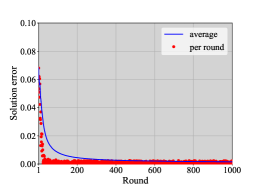
(a) $c_{100}$

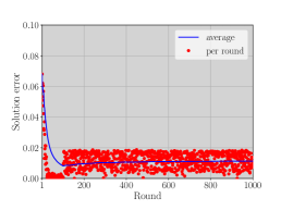
(b) $\frac{1}{100}\sum_{t=1}^{100}c_{t}$

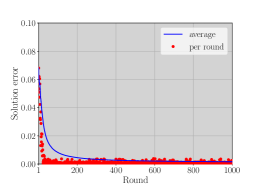
(c) Best $c_{t}$ out of $t=1,\ldots,100$

Figure 3: Comparison of the solution error for three policies to continue the optimization if the algorithm (here: MWU) receives no further update after $t=100$ rounds

To this end, we show in Figure 3 the solution error for the objectives produced by MWU for the case that there are no further updates after $100$ rounds. In Figure 3a, we use $c_{100}$ for the remaining $900$ rounds, in Figure 3b, we use $\frac{1}{100}\sum_{t=1}^{100}c_{t}$, in Figure 3c, it is the $c_{t}$ which produced the lowest error in the corresponding round $t$, over all rounds $t=1,\ldots,100$. We find that $c_{100}$ consistently produces solutions with a cost similar to that of the true objective and thus generalizes very well to the unseen data in this instance. The same holds for the best $c_{t}$, which in this case was highly non-unique, as there are many rounds where the error is $0$. Thus, we averaged over all $c_{t}$ with error $0$ and chose the resulting objective. In contrast, averaging over all $c_{t}$ from the first $100$ rounds performs much worse. Altogether, we conclude that our approach leads to objective functions which provide a consistent explanation for the observed decisions in settings with i.i.d. sampled parameters $p_{t}$ empirically, even for those observations which the algorithm has not seen before.

4.2 Learning Travel Times

In our second computational experiment, we consider a street network where the travel times on a segment may vary over the day. Each driver in the network is assumed to choose a route that leads from some origin to some destination in the shortest time possible. In other words, each driver solves a shortest-path problem on the same directed graph $G=(V,A)$. An observation $p_{t}=(p^{1}_{t},p^{2}_{t})$ for $t\in[T]$ represents a driver in the network who departs at a given time step in the observation period which we also denote by $t$, going from the starting point $p^{1}_{t}\in V$ to the end point $p^{2}_{t}\in V$. The entries of $x_{t}$ indicate the path taken by driver $t$, which are obtained by solving the following optimization problem $\textrm{OPT}(p_{t})$:

$$\min\>\>\>\> \sum_{a\in A}c_{\text{true},ta}x_{ta}$$

$$\mathrm{s.t.}\>\>\>\> \sum_{a\in\delta^{+}(v)}x_{ta}-\sum_{a\in\delta^{-}(v)}x_{ta} \;\;\;\,= \;\;\;\,\left\{\begin{array}[]{rl}1,&\text{if }v=p^{1}_{t}\\ -1,&\text{if }v=p^{2}_{t}\\ 0,&\text{otherwise}\end{array}\right. \quad\begin{array}[]{l}(\forall v\in V)\end{array}$$ (11)

$$x_{ta} \;\;\;\,\in \;\;\;\,\{0,1\}^{\lvert A\rvert}.$$ (13)

Observing the paths of each of the drivers, we want to learn the values $c_{\text{true},ta}$ corresponding to the travel times to traverse arc $a\in A$ at time step $t$. The major difference to our previous experiment is that here the objective function will be allowed to change over time, representing, for example, slowdowns due to traffic congestions.

We created instances of the problem based on a real-world street network, namely an aggregated version of the city map of Chicago. It is available as instance ChicacoSketch in Ben Stabler’s library of transportation networks (see Stabler, (2018)), and has 933 nodes and 2950 arcs (of which we ignore the 387 nodes representing “zones” as well as their incident arcs). Each arc $a$ has a certain free-flow time $c_{\text{free},a}$, which we assume to be the unknown uncongested travel time. For each driver $t$, we chose a random pair of an origin and a destination node. Furthermore, we consider 5 hours of real time and one driver per 5 minutes for creating the observations. Hence, our time horizon is $T=60$, which is also the number of drivers.

We consider three different settings. In a first step, we try to retain the free-flow times from the observed paths, i.e. we assume the travel times to be constant: $c_{\text{true},ta}\coloneqq c_{\text{free},a}$ for all $a\in A$ and $t=1,\ldots,T$. As a second test, we integrate temporary increases in the travel time induced by congestions on the most-frequently used arcs. These increases were modelled in the following way: we computed all shortest paths in the network between any two nodes and chose the top 5% of arcs with the highest number of shortest paths traversing them as bottlenecks. For each of these bottlenecks $a$, we chose the travel time at time step $t$ to be

$$c_{\text{true},ta}\coloneqq\begin{cases}c_{\text{free},a},&\text{otherwise},\ \ \ \ \ \ \ \ \ \ \ \ \ \ (\frac{t-6}{6})c_{\text{free},a},\ \ \ \ \ \text{if }t\in\{12,\ldots,18\},\\ 2c_{\text{free},a},&\text{if }t\in\{19,\ldots,29\},\ \ \ (\frac{42-t}{6})c_{\text{free},a},\ \ \ \ \text{if }t\in\{30,\ldots,36\}.\end{cases}$$

This means that at one hour of real time, the congestions on all bottleneck arcs $a$ start to build up and reach the maximal congestion within 30 minutes, staying on maximal congestion for one hour and then ebbing away within 30 minutes. Finally, we consider the case of abrupt changes in travel time as they might arise from roads which are suddenly blocked for some reason. To this end, we altered the travel times of the same arcs as before, but chose the travel time at time step $t$ as

$$c_{\text{true},ta}\coloneqq\begin{cases}1000c_{\text{free},a},&\text{if }t\in\{12,\ldots,36\},\quad c_{\text{free},a},\quad\text{otherwise.}\end{cases}$$

We then used MWU to learn the dynamically changing travel times.

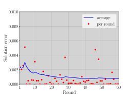
(a) No congestion

(b) Gradual congestion

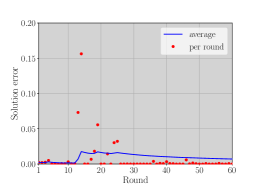
(c) Abrupt congestion

Figure 4: Solution error for each round (red) and averaged up to the current round (blue) for the shortest-path problem with $T=60$ drivers under the different congestion scenarios for MWU

Figure 4 depicts the solution error for the three cases. From Figure 4a, we can see that we achieve a very good convergence of the error already with as few as 60 observations. For a gradually building and receding congestion, we see in Figure 4b that the performance of our algorithm nearly does not deterioriate at all, which means the learned objective quickly adapts to the slowly changing travel times. In the case of abrupt congestions, we see the error spiking sharply at the point where the congestions begin, but quickly declining afterwards. After 60 rounds, the average solution error is still about 8 times higher than in the unpertubed case, which means it takes some time to recover. This behaviour is expected, as our theoretical results predict the washing out of any error $d$ in the average regret at a rate of $\mathcal{O}(d/\sqrt{T})$, cf. the discussion of Lemma 3.13. Nevertheless, the solutions we obtain from round 26 on have a loss which is significantly below the average regret. To summarize, this experiment shows that we can learn to take efficient decisions already with few observations at hand and that we can quite easily cope with small continuing changes or big but seldom changes in the target objective.

4.3 Learning Optimal Delivery Routes

Finally, we demonstrate the potential of OGD to learn objective coefficients with mixed signs. For this purpose, we consider a simple delivery problem where a company has certain customers which it serves from its depot. The delivery network is given by a complete undirected graph $G=(V\cup\{v_{0}\},E)$ with a designated node $v_{0}$ representing the depot and the nodes in $V$ representing the customers. A delivery route consists of a Hamilton tour comprising the depot as well as the subset of customers the company decides to serve in the given time step and in its preferred order. We assume that each edge $e\in E$ has a cost $c_{te}$ for traversing it, and that each customer $v\in V$ brings a revenue $r_{tv}$ if served, both unknown and varying over time steps $t\in[T]$. This uncertainty might for example arise from different traffic scenarios affecting delivery costs as well as different customer demand scenarios. Altogether, the company wants to solve the following profitable tour problem $\textrm{OPT}(p_{t})$, a prize-collecting variant of the travelling salesman problem, for each $t\in[T]$:

$$\max\>\>\>\> \sum_{v\in V}r_{tv}y_{tv}-\sum_{e\in E}c_{te}x_{te}$$

$$\mathrm{s.t.}\>\>\>\> \sum_{e\in\delta(v)}x_{te} \;\;\;\,= \;\;\;\,2y_{tv} \quad\begin{array}[]{l}(\forall v\in V\cup\{v_{0}\})\end{array}$$ (15)

$$\sum_{\begin{subarray}{c}e=(i,j)\in E:\\ i,j\in S\end{subarray}}x_{te}+y_{l} \;\;\;\,\leq \;\;\;\,1+\sum_{i\in S\setminus\{k\}}y_{i} \quad\begin{array}[]{l}\\ (\forall S\subset V\cup\{v_{0}\},2\leq\lvert S\rvert\leq\lvert V\rvert-1)\\ (\forall k\in S)(\forall l\notin S)\end{array}$$ (19)

$$y_{tv} \;\;\;\,\leq \;\;\;\,y_{tv_{0}} \quad\begin{array}[]{l}(\forall v\in V)\end{array}$$ (21)

$$x_{t} \;\;\;\,\in \;\;\;\,\{0,1\}^{\lvert E\rvert}$$ (23)

$$y_{tv} \;\;\;\,\in \;\;\;\,\{0,1\}^{\lvert V\rvert+1},$$ (25)

where $x$ models the chosen edges and $y$ the chosen customers.

For our computational experiment, we use instance berlin52-gen3-50 from Gorka Kobeaga’s OPLib, see Kobeaga, (2018), where we scale up the customer revenues by a factor of 4 to yield a non-trivial trade-off against the edge costs. Then, in each time step $t\in[T]$, we draw the edge costs uniformly from an interval of $\pm$ 10% and the customer revenues from an interval of $\pm$ 20% around these basic values which we interpret as the expected costs and revenues respectively. Thus, we want to learn to distinguish the more efficient routes from the less efficient routes and the more profitable customers from the less profitable customers. We choose $F$ to be the unit cube and $c_{1}$ as the zero vector to initialize the OGD algorithm.

Figure 5 shows the results of the experiment.

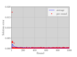
(a) Solution error

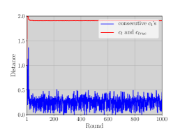
(b) $1$-norm objective distances

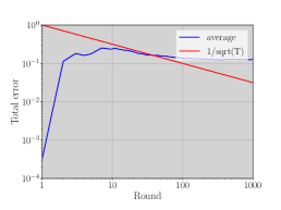
(c) Convergence

Figure 5: Solution error, objective distances and convergence for the prize-collecting travelling salesman problem for OGD

In Figure 5a, we see that the solution error falls relatively quickly after few iterations as for the other two problems. However, now the average regret does not converge to zero, but rather to the variance in the true objective which is sampled anew in each round. This is explainable by the dynamic nature of the objective function to be learned, cf. Lemma 3.13 and the corresponding discussion. We obtain a kind of “robust” objective, which tries to explain the observations produced by an actually non-constant target objective.

5 Final Remarks

We saw that algorithms derived from online-learning methods are capable of learning objective functions from optimal (and close-to-optimal) observed decisions, given knowledge of the underlying feasible set in each case. Especially, our framework provides a new online analogue of the established concept of inverse optimization, where the unknown objective may be determined via multiple samples and over time, with decisions taken in between the observations. We were able to prove that our algorithms achieve low errors with respect to the decisions based on the learned objectives. Furthermore, they are applicable in more general situations than previous methods, which required convexity of the feasible region, and they are usable in situations where the observations arrive online as a data stream, allowing to learn objectives which change over time. In computational experiments, we demonstrated that they quickly converge in practical settings, learning objectives which explain the observed decisions very well, including when testing them out-of-sample. The practical importance of this approach is evident when considering that much effort is made to come to procedures that automate model building from data. An important question in this respect is to what extent our framework can be extended to the learning of constraints (and objective functions simultaneously).

Appendix A Counterexample for the Follow-the-Leader Algorithm

In the following, we give a counterexample where the follow-the-leader scheme presented in Section 3.4 does not yield a strategy with sublinear regret.

Example A.1.

Consider the following series of feasible sets $X(p_{t})$ over rounds $t=1,\ldots,T$ for some time horizon $T>0$:

$$X(p_{t})\coloneqq\{(x_{1},x_{2})^{\top}\in\mathbbm{R}_{+}^{2}\mid x_{2}=1-\frac{1}{a_{t}}\},\quad\text{where}\quad a_{t}\coloneqq\sum_{\tau\in[t]}\left(\frac{1}{2}\right)^{\tau-1}.$$

They represent line segements going from $(0,1)^{\top}$ to $(a_{t},0)^{\top}$ in round $t$, approaching the line segment from $(0,1)^{\top}$ to $(2,0)^{\top}$ with $T\to\infty$. The true objective to learn shall be $c_{\text{true}}=(0,1)^{\top}$ and $F=\Delta_{2}$. In this setting, the optimal solution of the adversary will always be $(0,1)^{\top}$. Assuming that the player chooses objective $c_{1}=(1,0)^{\top}$ in the first round, the solution in that round will be $\bar{x}_{t}=(1,0)^{\top}$, while the adversary will play $x_{t}=(0,1)^{\top}$. In the next round, the player will thus have to play an objective whose angle to $(1,0)$ is at least as high as that between $(1,1)^{\top}$ and $(1,0)^{\top}$, i.e. a $c_{2}=(\gamma,1-\gamma)^{\top}$ with $\frac{1}{2}\leq\gamma\leq 1$. If, in general, the player chooses $c_{t}=(1/(1+a_{t-1}),a_{t-1}/(1+a_{t-1}))^{\top}$ in each round $t>1$, the point $(0,1)^{\top}$ will always be an optimal solution for all previously observed feasible sets $X(p_{t})$, but $(a_{t},0)^{\top}$ will be picked as the optimal solution in the current round. The player thus yields a regret of

$$\sum_{t\in[T]}c_{t}^{\top}(\bar{x}_{t}-x_{t})-\sum_{t\in[T]}c_{\text{true}}^{\top}(\bar{x}_{t}-x_{t}) =\sum_{t\in[T]}\begin{pmatrix}\frac{1}{1+a_{t-1}}\\ \frac{a_{t-1}}{1+a_{t-1}}\end{pmatrix}^{\top}\begin{pmatrix}a_{t}\\ -1\end{pmatrix}-\sum_{t\in[T]}\begin{pmatrix}0\\ 1\end{pmatrix}^{\top}\begin{pmatrix}a_{t}\\ -1\end{pmatrix}$$

$$=\sum_{t\in[T]}\frac{a_{t}-a_{t-1}}{1+a_{t-1}}-\sum_{t\in[T]}(-1)$$

$$=\sum_{t\in[T]}\frac{1}{2(1+a_{t-1})}+T\geq\sum_{t\in[T]}\frac{1}{6}+T=\frac{7T}{6},$$

such that neither of objective error, solution error or total error converges to zero on average with $T\to\infty$.

Appendix B Additional Results for the Knapsack Problem

Here, we give additional results for the linear and integer knapsack problem studied in Section 4.1

In Table 2, we show statistics on the computational results for the linear knapsack problem. It shows the arithmetic means and standard deviations of the average errors after 5, 50 and 500 iterations for each of the algorithms, with the arithmetic mean taken over all 50 instances.

Algorithm	MWU			OGD			LP
# Rounds	5	50	500	5	50	500	5	50	500
$\varnothing$ objective error	0.21	0.03	0.01	0.23	0.04	$<$0.01	0.15	0.03	$<$0.01
$\sigma$ objective error	0.03	$<$0.01	$<$0.01	0.04	$<$0.01	$<$0.01	0.08	0.01	$<$0.01
$\varnothing$ solution error	0.06	0.02	$<$0.01	0.06	0.01	$<$0.01	0.29	0.16	0.03
$\sigma$ solution error	0.01	$<$0.01	$<$0.01	0.01	$<$0.01	$<$0.01	0.11	0.04	0.02
$\varnothing$ total error	0.27	0.05	0.01	0.28	0.05	0.01	0.44	0.18	0.04
$\sigma$ total error	0.05	0.01	$<$0.01	0.05	0.01	$<$0.01	0.11	0.04	0.02

Table 2: Mean and standard deviation of the average errors for the linear knapsack problem with $n=50$ items and $T=500$ observations for each algorithm, rounded to two decimals, with the arithmetic mean taken over 50 runs on random instances

As can be seen, after few iterations we obtain error values close to zero for MWU und OGD, with standard deviations lowering quickly over the number of rounds played. Both perform notably better in early iterations than LP, which is, however, able to catch up, as after a couple of rounds the total error is basically always zero.

In Figure 6, the objective error, solution and total error, are shown for MWU, OGD and LP.

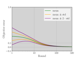
(a) Objective error for MWU

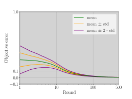
(b) Objective error for OGD

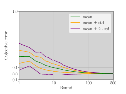
(c) Objective error for LP

(d) Solution error for MWU

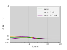
(e) Solution error for OGD

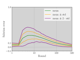
(f) Solution error for LP

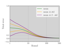
(g) Total error for MWU

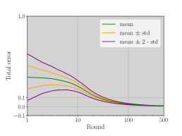
(h) Total error for OGD

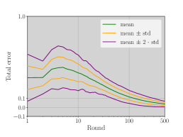
(i) Total error for LP

Figure 6: The arithmetic means and standard deviations of the different error types in each round (red) and averaged up to the current round (blue) for the linear knapsack problem with $n=50$ items over $T=500$ rounds for each of the three algorithms, with the arithmetic mean taken over 500 runs, on a doubly symmetric-logarithmic plot

As can be seen, in general after few iterations the error values reside close to zero, and the standard deviations lower quickly with the number of rounds played. The pictures for MWU and OGD are almost indistinguishable, while the mean average errors for LP are on a somewhat larger scale due to the tendentially higher errors in the very first rounds.

Figure 7 shows plots of the solution error, depicting both the error in a given round $t$ and the average total error up to round $t$ for the integer knapsack problem.

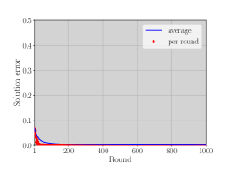
(a) MWU

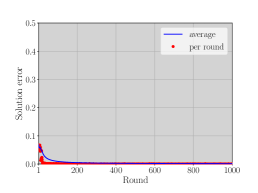
(b) OGD, fixed learning rate

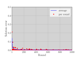
(c) OGD, dynamic learning rate

Figure 7: The solution error for each round (red) and averaged up to the current round (blue) for the integer knapsack problem with $n=1000$ items over $T=1000$ rounds for MWU and two variants of OGD

Again, the average errors fall quickly, and only few of the errors in individual rounds, mainly in the first rounds, deviate beyond the average.

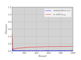
(a) MWU

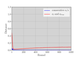
(b) OGD, fixed learning rate

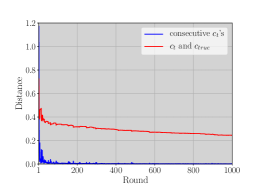
(c) OGD, dynamic learning rate

Figure 8: Distance in the $1$-norm between two consecutive objective objective functions (blue) and between the objective function in the current round and the true objective function (red) for the integer knapsack problem

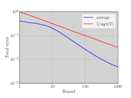
(a) MWU

(b) OGD, fixed learning rate

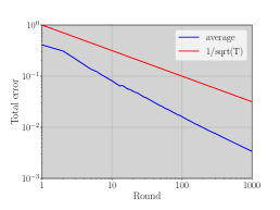
(c) OGD, dynamic learning rate

Figure 9: Doubly logarithmic plot of the average total error (blue) for the integer knapsack problem against the function $f(T)=1/\sqrt{T}$ (red)

In Figure 8, it is visible at first sight that empirically the learned objective does not converge to the true objective function. In the case of MWU, the distance to the true objective function converges to about $0.1$. For OGD with fixed learning rate $\eta=D/G\sqrt{T}$, the behaviour is very similar. When we choose the dynamic learning rate $\eta_{t}=D/G\sqrt{t}$, with a higher scale of the updates at the beginning, the convergence is slower by a factor two, which is in line with our treatment of the choice of learning rates in Section 3.3.

Finally, Figure 9 shows the MWA and two OGD algorithms for the integer knapsack, depicting the average total error up to a given round versus the asymptotic upper bound represented by the function $f(T)=1/\sqrt{T}$ on a log-log-scale. What we observe is that – over the total observation horizon – the order of convergence is basically same as that of $f$, where, again, all algorithms perform about equally well.

Appendix C Visualization of the Solution for the Learning of Travels Times

In the following, we give a visualization of the solutions produced by the original as well as the learned objective functions for the problem of learning travel times presented in Section 4.2. Figure 10a shows the graph corresponding to the Chicago street network, where we have only plotted the arcs which were actually used in a any of the shortest paths over 60 rounds, assuming the constant free-flow objective. The darker an arc is coloured, the higher is the number of actually taken paths which it is part of. We can clearly recognize several highways as well as shortcuts through the city center. In Figure 10b, we show the same figure, but with the paths learned by MWU without congestions. We see that the algorithm chooses a couple of routes which would not be chosen according to the true objective, expectably at the beginning, as it first needs to learn which ones are the good arcs (starting from the assumption that all arcs are of equal travel time). We clearly observe that the most-frequently used arcs are the same ones as with the true objective. The same holds for the cases of gradual and abrupt congestions, shown in Figures 10c and 10d respectively, with the exception that the most-frequent arcs are not chosen as often, as they take longer to traverse or are even blocked for a considerable amount of time. Instead, a few arcs belonging to detours become more interesting. This shows that our algorithm quickly adapt even after a major shift in the learning target.

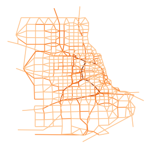
(a) True objective

(b) No congestion

(c) Gradual congestion

(d) Abrupt congestion

Figure 10: Actual paths taken in the network for the true objective and the objectives learned by MWU under the three different congestion types

References

- Abbasi-Yadkori et al., (2011) Abbasi-Yadkori, Y., Pál, D., and Szepesvári, C. (2011). Improved algorithms for linear stochastic bandits. In Advances in Neural Information Processing Systems 24, pages 2312–2320. Curran Associates, Inc.
- Ahuja and Orlin, (2000) Ahuja, R. K. and Orlin, J. B. (2000). A faster algorithm for the inverse spanning tree problem. Journal of Algorithms, 34(1):177–193.
- Arora et al., (2012) Arora, S., Hazan, E., and Kale, S. (2012). The multiplicative weights update method: A meta-algorithm and applications. Theory of Computing, 8:121–164.
- Aswani et al., (2018) Aswani, A., Shen, Z.-J. M., and Siddiq, A. (2018). Inverse optimization with noisy data. Operations Research, 66(3):870–892.
- Audibert et al., (2013) Audibert, J.-Y., Bubeck, S., and Lugosi, G. (2013). Regret in online combinatorial optimization. Mathematics of Operations Research, 39(1):31–45.
- Bertsimas and Kallus, (2016) Bertsimas, D. and Kallus, N. (2016). Pricing from observational data. Technical report, Massachusetts Institute of Technology.
- Burton and Toint, (1992) Burton, D. and Toint, P. L. (1992). On an instance of the inverse shortest paths problem. Mathematical Programming, 53(1):45–61.
- Burton and Toint, (1994) Burton, D. and Toint, P. L. (1994). On the use of an inverse shortest paths algorithm for recovering linearly correlated costs. Mathematical Programming, 63(1):1–22.
- Bärmann et al., (2020) Bärmann, A., Martin, A., Pokutta, S., and Schneider, O. (2020). Supplementary materials: An online learning approach to inverse optimization.
- Bärmann et al., (2017) Bärmann, A., Pokutta, S., and Schneider, O. (2017). Emulating the expert: Inverse optimization through online learning. In Proceedings of the 34th International Conference on Machine Learning, volume 70 of Proceedings of Machine Learning Research, pages 400–410. PMLR. Available at: http://proceedings.mlr.press/v70/barmann17a.html.
- Cesa-Bianchi and Lugosi, (2006) Cesa-Bianchi, N. and Lugosi, G. (2006). Prediction, learning, and games. Cambridge University Press.
- Chan et al., (2019) Chan, T. C. Y., Lee, T., and Terekhov, D. (2019). Inverse optimization: Closed-form solutions, geometry, and goodness of fit. Management Science.
- Chen et al., (2015) Chen, X., Owen, Z., Pixton, C., and Simchi-Levi, D. (2015). A statistical learning approach to personalization in revenue management. Technical report, New York University.
- D. Burton, (1997) D. Burton, W. R. Pulleyblank, P. L. T. (1997). Network Optimization, chapter The Inverse Shortest Paths Problem with Upper Bounds on Shortest Paths Costs, pages 156–171. Springer.
- Dani et al., (2008) Dani, V., Hayes, T. P., and Kakade, S. M. (2008). Stochastic linear optimization under bandit feedback. In Conference on Learning Theory (COLT).
- den Hertog and Postek, (2016) den Hertog, D. and Postek, K. (2016). Bridging the gap between predictive and prescriptive analytics – new optimization methodology needed. Technical report, Tilburg University, Netherlands.
- Dong et al., (2018) Dong, C., Chen, Y., and Zeng, B. (2018). Generalized inverse optimization through online learning. In Bengio, S., Wallach, H., Larochelle, H., Grauman, K., Cesa-Bianchi, N., and Garnett, R., editors, Advances in Neural Information Processing Systems 31, pages 86–95. Curran Associates, Inc.
- Esfahani et al., (2018) Esfahani, P. M., Shafieezadeh-Abadeh, S., Hanasusanto, G. A., and Kuhn, D. (2018). Data-driven inverse optimization with imperfect information. Mathematical Programming, 167(1):191–234.
- Freund and Schapire, (1997) Freund, Y. and Schapire, R. E. (1997). Adaptive game playing using multiplicative weights. Games and Economic Behavior, 29:79–103.
- Gurobi Optimization, Inc., (2018) Gurobi Optimization, Inc. (2018). Gurobi optimizer reference manual.
- Hannan, (1957) Hannan, J. (1957). Approximation to bayes risk in repeated play. In Contributions to the Theory of Games, volume 3, pages 97–139. Princeton University Press.
- Hazan, (2016) Hazan, E. (2016). Introduction to Online Convex Optimization. Now Publishers, Inc.
- Iyengar and Kang, (2005) Iyengar, G. and Kang, W. (2005). Inverse conic programming with applications. Operations Research Letters, 33(3):319–330.
- Kalai and Vempala, (2005) Kalai, A. and Vempala, S. (2005). Efficient algorithms for online decision problems. Journal of Computer and System Sciences, 71:291–307.
- Kallus and Udell, (2015) Kallus, N. and Udell, M. (2015). Learning preferences from assortment choices in a heterogeneous population. Technical report, Massachusetts Institute of Technology.
- Kallus and Udell, (2016) Kallus, N. and Udell, M. (2016). Dynamic assortment personalization in high dimensions. Technical report, Cornell University.
- Keshavarz et al., (2011) Keshavarz, A., Wang, Y., and Boyd, S. (2011). Imputing a convex objective function. In Proceedings of the 2011 IEEE International Symposium on Intelligent Control (ISIC), pages 613–619.
- Kobeaga, (2018) Kobeaga, G. (2018). OPLib. Available at: https://github.com/bcamath-ds/OPLib.
- Konstantakopoulos et al., (2016) Konstantakopoulos, I. C., Ratliff, L. J., Jin, M., Spanos, C., and Sastry, S. S. (2016). Smart building energy efficiency via social game: A robust utility learning framework for closing-the-loop. In 2016 1st International Workshop on Science of Smart City Operations and Platforms Engineering (SCOPE) in partnership with Global City Teams Challenge (GCTC) (SCOPE - GCTC), pages 1–6.
- Li, (2016) Li, J. Y.-M. (2016). Inverse optimization of convex risk functions. Technical report, University of Ottawa, Canada.
- Littlestone and Warmuth, (1994) Littlestone, N. and Warmuth, M. K. (1994). The weighted majority algorithm. Information and Computation, 108:212–261.
- Lodi, (2016) Lodi, A. (2016). Big data & mixed-integer (nonlinear) programming. Presentation, available at: https://atienergyworkshop.files.wordpress.com/2015/11/andrealodi.pdf.
- Molloy et al., (2016) Molloy, T. L., Tsai, D., Ford, J. J., and Perez, T. (2016). Discrete-time inverse optimal control with partial-state information: A soft-optimality approach with constrained state estimation. In 2016 IEEE 55th Conference on Decision and Control (CDC), pages 1926–1932.
- Nemirovski, (1979) Nemirovski, A. (1979). Efficient methods for large-scale convex optimization problems. Ekonomika i Matematicheskie Metody, 15.
- Nielsen and Jensen, (2004) Nielsen, T. D. and Jensen, F. V. (2004). Learning a decision makers’s utility function from (possibly) inconsistent behavior. Artificial Intelligence, 160:53–78.
- Panchea and Ramdani, (2015) Panchea, A. M. and Ramdani, N. (2015). Towards solving inverse optimal control in a bounded-error framework. In 2015 American Control Conference (ACC), pages 4910–4915.
- Papadopoulos et al., (2016) Papadopoulos, A. V., Bascetta, L., and Ferretti, G. (2016). Generation of human walking paths. Autonomous Robots, 40(1):55–75.
- Pisinger, (2005) Pisinger, D. (2005). Where are the hard knapsack problems? Computers & Operations Research, 32(9):2271–2284.
- Plotkin et al., (1995) Plotkin, S. A., Shmoys, D. B., and Éva Tardos (1995). Fast approximation algorithms for fractional packing and covering problems. Mathematics of Operations Research, 20(2):257–301.
- Qiang and Bayati, (2016) Qiang, S. and Bayati, M. (2016). Dynamic pricing with demand covariates. Technical report, Stanford University.
- Ratia et al., (2012) Ratia, H., Montesano, L., and Martinez-Cantin, R. (2012). On the performance of maximum likelihood inverse reinforcement learning.
- Ratliff et al., (2014) Ratliff, L. J., Dong, R., Ohlsson, H., and Sastry, S. S. (2014). Incentive design and utility learning via energy disaggregation. IFAC Proceedings Volumes.
- Sayre and Ruan, (2014) Sayre, G. A. and Ruan, D. (2014). Automatic treatment planning with convex imputing. Journal of Physics: Conference Series, 489(1).
- Schaefer, (2009) Schaefer, A. (2009). Inverse integer programming. Optimization Letters, 3(4):483–489.
- Sessa et al., (2020) Sessa, P. G., Bogunovic, I., Kamgarpour, M., and Krause, A. (2020). Mixed strategies for robust optimization of unknown objectives. Technical report, Eidgenössische Technische Hochschule Zürich.
- Shalev-Shwartz et al., (2012) Shalev-Shwartz, S. et al. (2012). Online learning and online convex optimization. Foundations and Trends® in Machine Learning, 4(2):107–194.
- Simchi-Levi, (2014) Simchi-Levi, D. (2014). OM research: From problem-driven to data-driven research. Manufacturing & Service Operations Management, 16(1):2–10.
- Sokkalingam et al., (1999) Sokkalingam, P. T., Ahuja, R. K., and Orlin, J. B. (1999). Solving inverse spanning tree problems through network flow techniques. Operations Research, 47(2):291–298.
- Stabler, (2018) Stabler, B. (2018). Transportation networks. Available at: https://github.com/bstabler/TransportationNetworks.
- Syed and Schapire, (2007) Syed, U. and Schapire, R. E. (2007). A game-theoretic approach to apprenticeship learning. In Conference on Neural Information Processing System (NIPS).
- Thai and Bayen, (2018) Thai, J. and Bayen, A. M. (2018). Imputing a variational inequality function or a convex objective function: A robust approach. Journal of Mathematical Analysis and Applications, 457(2):1675–1695.
- Troutt et al., (2011) Troutt, M. D., Gwebu, K. L., Wang, J., and Brandyberry, A. A. (2011). Some experiments on subjective optimisation. International Journal of Operational Research, 12(1):79–103.
- Troutt et al., (2006) Troutt, M. D., Pang, W.-K., and Hung-Huo, S. (2006). Behavioral estimation of mathematical programming objective function coefficients. Management Science, 52(3):422–434.
- Troutt et al., (2005) Troutt, M. D., Tadisina, S. K., Sohn, C., and Brandyberry, A. A. (2005). Linear programming system identification. European Journal on Operational Research, 161:663–672.
- Vovk, (1990) Vovk, V. G. (1990). Aggregating strategies. In Conference on Learning Theory (COLT).
- Ward et al., (2019) Ward, A., Master, N., and Bambos, N. (2019). Learning to emulate an expert projective cone scheduler. In 2019 American Control Conference (ACC), pages 292–297.
- Yang et al., (2014) Yang, I., Zeilinger, M. N., and Tomlin, C. J. (2014). Utility learning model predictive control for personal electric loads. In 53rd IEEE Conference on Decision and Control, pages 4868–4874.
- Zinkevich, (2003) Zinkevich, M. (2003). Online convex programming and generalized infinitesimal gradient ascent. Technical report, School of Computer Science, Carnegie Mellon University.