R³SGM: Real-time Raster-Respecting Semi-Global Matching for Power-Constrained Systems

Abstract

Stereo depth estimation is used for many computer vision applications. Though many popular methods strive solely for depth quality, for real-time mobile applications (e.g. prosthetic glasses or micro-UAVs), speed and power efficiency are equally, if not more, important. Many real-world systems rely on Semi-Global Matching (SGM) to achieve a good accuracy vs. speed balance, but power efficiency is hard to achieve with conventional hardware, making the use of embedded devices such as FPGAs attractive for low-power applications. However, the full SGM algorithm is ill-suited to deployment on FPGAs, and so most FPGA variants of it are partial, at the expense of accuracy. In a non-FPGA context, the accuracy of SGM has been improved by More Global Matching (MGM), which also helps tackle the streaking artifacts that afflict SGM. In this paper, we propose a novel, resource-efficient method that is inspired by MGM’s techniques for improving depth quality, but which can be implemented to run in real time on a low-power FPGA. Through evaluation on multiple datasets (KITTI and Middlebury), we show that in comparison to other real-time capable stereo approaches, we can achieve a state-of-the-art balance between accuracy, power efficiency and speed, making our approach highly desirable for use in real-time systems with limited power.

I Introduction

Numerous computer vision applications, including 3D voxel scene reconstruction [35, 14], object recognition [25], 6D camera relocalisation [43, 4], and autonomous navigation [31, 16], either rely on, or can benefit from, the availability of depth to capture 3D scene structure. Active approaches for acquiring depth, based on structured light [51] or LiDAR, produce high-quality results. However, the former performs poorly outdoors, where sunlight washes out the infrared patterns it uses, whereas the latter is generally expensive and power-hungry, whilst simultaneously only producing sparse depth. Significant attention has thus been devoted to passive methods of obtaining dense depth from either monocular or stereo images. Although recent approaches based on deep learning [27, 13] have made progress in the area, monocular approaches, which only require a single camera, struggle in determining scale [45]. Stereo approaches, as a result, are often preferred when multiple cameras can be used, with binocular stereo methods (which achieve a compromise between quality and cost) proving particularly popular.

Many binocular stereo methods estimate disparity by finding correspondences between the two images. They typically involve four phases [39]: (a) matching cost computation, (b) cost aggregation, (c) disparity optimisation, and (d) disparity refinement. At a high level, such methods can be classified into two categories, based on the subset of steps mentioned above that they focus on performing effectively, and the amount of information used to estimate the disparity for each pixel:

1. Local methods [7, 21, 22] focus on steps (a) and (b), finding correspondences between pixels in the left and right images by matching simple, window-based features across the disparity range. Whilst fast and computationally cheap, they suffer in textureless/repetitive areas, and can easily estimate incorrect disparities.

2. Global methods [44, 23, 3, 5], by contrast, are better suited to estimating accurate depths in those areas, since they enforce smoothness over disparities via the (possibly approximate) minimisation of an energy function defined over the whole image (they focus on steps (c) and (d)). However, this increased accuracy tends to come at a high computational cost, making these methods unsuitable for real-time applications.

Semi-global matching (SGM) [17] bridges the gap between local and global methods: by approximating the global methods’ image-wide smoothness constraint with the sum of several directional minimisations over the disparity range (usually 8 or 16 directions, in a star-shaped pattern), it produces reasonable depth in a fraction of the time. It has thus proved highly popular in real-world systems, and many FPGA-based approaches have been inspired by it [10, 2, 41, 20, 42, 28]. Other FPGA-based methods have also been presented [50, 37, 46, 34, 36], but, whilst typically faster than those inspired by SGM, they seldom reach the same level of accuracy. However, because the disparities that SGM computes for neighbouring pixels are based on star-shaped sets of input pixels that are mostly disjoint, SGM suffers from streaking in areas in which the data terms in some directions are weak, whilst those in other directions are strong. Recently, this problem has been partially addressed by an approach called More Global Matching (MGM) [9], which incorporates information from two directions into each of SGM’s directional minimisations; however, because this work was not designed with FPGAs in mind, it cannot be applied straightforwardly in an embedded context (it requires multiple passes over the pixels in the input images, several of them in non-raster order, to compute the bi-directional energies to be minimised).

In this paper, we present an approach inspired by MGM [9] that is much more amenable to real-time FPGA implementation, whilst achieving similar accuracy and much lower power consumption. We replace the multiple bi-directional minimisations of MGM, some of which cannot be computed in raster order, with a single four-directional minimisation based only on pixels that are available when processing the image as a stream. This allows us to process each image in raster order and in a single pass, allowing us to stream data directly from a camera connected to the FPGA and output disparity values without requiring an intermediate buffering stage, simplifying the system architecture and reducing latency.

This paper is structured as follows. In Section II, we review SGM [17] and MGM [9], the algorithms that inspired our work. In Section III, we describe our method, and show how to implement it on an FPGA. Finally, in Section IV, we evaluate our method’s accuracy on the KITTI [11, 29, 30] and Middlebury [38] datasets, and examine its power consumption and FPGA resource usage. By comparing it to other real-time stereo methods, we show that it achieves a state-of-the-art balance between accuracy, speed and power efficiency, making it desirable for use in real-time low-power systems.

II Background

II-A Semi-Global Matching (SGM)

(a)

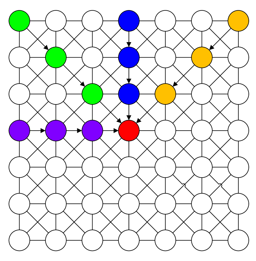
(b)

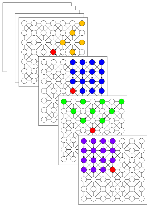
(c)

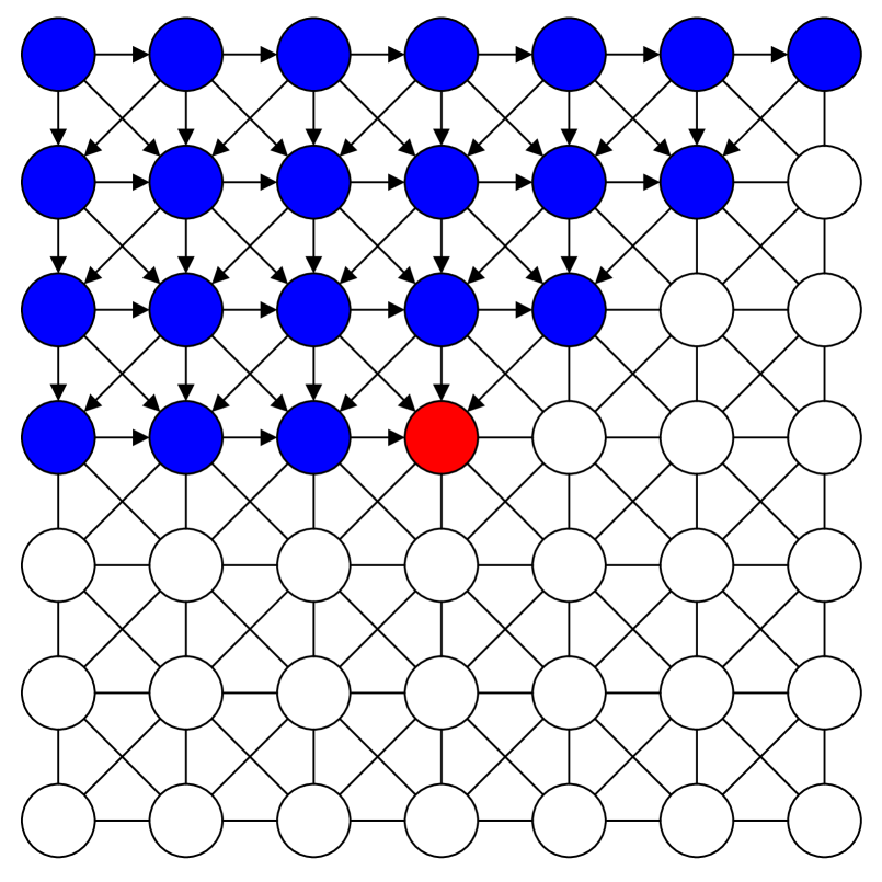
(d)

Figure 1: The pixels used to compute $L_{\mathbf{r}}(\mathbf{p},\cdot)$ for pixel $\mathbf{p}$ (in red) and each scan line $\mathbf{r}$, for (1(a)) a full implementation of SGM (Section II-A), and (1(b)) a typical raster-based FPGA implementation of SGM (Section II-A1). Each non-red colour denotes a distinct scan line. In (1(c)), we show the pixels that MGM would use for the same scan lines (Section II-B). Finally, in (1(d)), we show the pixels used to compute our single cost term, allowing us to estimate disparities whilst processing pixels in a streaming fashion (note that to compute the cost vector associated with the red pixel, we require the cost vectors only from pixels that precede it in raster order). See Section III for more details.

SGM [17] is a popular stereo matching method, owing to the good balance it achieves between accuracy and computational cost. As per [8], it aims to find a disparity map $D$ that minimises the following energy function, defined on an undirected graph $G=(I,\mathcal{E})$, with $I$ the image domain and $\mathcal{E}$ the set of edges defined by the 8-connectivity rule:

$$E(D)=\sum_{\mathbf{p}\in I}C_{\mathbf{p}}(D(\mathbf{p}))+\sum_{\{\mathbf{p},\mathbf{q}\}\in\mathcal{E}}V(D(\mathbf{p}),D(\mathbf{q}))$$ (1)

Each unary term $C_{\mathbf{p}}(D(\mathbf{p}))$ denotes the ‘matching cost’ of assigning pixel $\mathbf{p}$ in the left image the disparity $D(\mathbf{p})\in\mathcal{D}=\left[0,d_{\max}\right]$. This would match it with pixel $\mathbf{p}-D(\mathbf{p})\,\mathbf{i}$ in the right image, where $\mathbf{i}=[1,0]^{\top}$. Different matching cost functions were evaluated in [1, 19]. The choice is typically based on (i) the desired invariances to nuisances (e.g. changes in illumination) and (ii) computational requirements. Each pairwise term $V(D(\mathbf{p}),D(\mathbf{q}))$ encourages smoothness by penalising disparity variations between neighbouring pixels:

$$V(d,d^{\prime})=\begin{cases}0&\mbox{if }d=d^{\prime}\\ P_{1}&\mbox{if }|d-d^{\prime}|=1\\ P_{2}&\mbox{otherwise}\end{cases}$$ (2)

The penalty $P_{1}$ is typically smaller than $P_{2}$, to avoid over-penalising gradual disparity changes, e.g. on slanted or curved surfaces. By contrast, $P_{2}$ tends to be larger, so as to more strongly discourage significant jumps in disparity.

Since the minimisation problem posed by Equation 1 is NP-hard, SGM approximates its solution by splitting it into several independent 1D problems defined along scan lines. More specifically, it associates each pixel $\mathbf{p}$ in the image with 8 scan lines, each of which follows one of the cardinal directions ($0\mathrm{°}$, $45\mathrm{°}$, $\ldots$, $315\mathrm{°}$), as per 1(a). We can denote these scan lines as a vector set $R\subseteq\mathbb{R}^{2}$:

$$R=\Bigl{\{} \scriptsize\left[\begin{array}[]{c}1\\ 0\end{array}\right],\left[\begin{array}[]{c}1\\ 1\end{array}\right],\left[\begin{array}[]{c}0\\ 1\end{array}\right],\left[\begin{array}[]{c}-1\\ 1\end{array}\right],$$ (3)

$$\scriptsize\left[\begin{array}[]{c}-1\\ 0\end{array}\right],\left[\begin{array}[]{c}-1\\ -1\end{array}\right],\left[\begin{array}[]{c}0\\ -1\end{array}\right],\left[\begin{array}[]{c}1\\ -1\end{array}\right]\Bigr{\}}.$$

Each pixel $\mathbf{p}$ is then associated with a directional cost $L_{\mathbf{r}}(\mathbf{p},d)$ for each direction $\mathbf{r}\in R$ and each disparity $d$. These costs can be computed recursively via

$$L_{\mathbf{r}}(\mathbf{p},d)=C_{\mathbf{p}}(d)\;+ \min_{d^{\prime}\in\mathcal{D}}\left(L_{\mathbf{r}}(\mathbf{p}-\mathbf{r},d^{\prime})+V(d,d^{\prime})\right)$$ (4)

$$- \min_{d^{\prime}\in\mathcal{D}}L_{\mathbf{r}}(\mathbf{p}-\mathbf{r},d^{\prime}),$$

in which $\mathbf{p}-\mathbf{r}$ refers to the pixel preceding $\mathbf{p}$ along the scan line denoted by $\mathbf{r}$. The minimum $L_{\mathbf{r}}$ cost associated with $\mathbf{p}-\mathbf{r}$ is subtracted from all costs computed for $\mathbf{p}$ to prevent them growing without bound as the distance from the image edge increases [17]. Having computed the directional costs, SGM then sums them to form an aggregated cost volume:

$$L(\mathbf{p},d)=\sum_{\mathbf{r}\in R}L_{\mathbf{r}}(\mathbf{p},d)$$ (5)

Finally, it selects each pixel’s disparity using a Winner-Takes-All (WTA) approach to estimate a disparity map $D^{*}$:

$$D^{*}(\mathbf{p})=\operatorname*{argmin}_{d\in\mathcal{D}}\;L(\mathbf{p},d)$$ (6)

The disparities estimated by SGM only approximate the solution of the initial problem, for which we would need to enforce a smoothness term over the whole image grid, but they are much less demanding to compute and, despite causing streaking artifacts in the final disparity image, have been proven to be accurate enough for practical purposes [18].

One technique commonly used to filter out incorrect disparity values is to perform an LR consistency check [17], which involves computing the disparities not just of pixels in the left image, but also in the right image, and checking that the two match (e.g. that if $\mathbf{p}$ in the left image has disparity $d$, then so does pixel $\mathbf{p}-d\mathbf{i}$ in the right image). Observe that the disparities of pixels in the right image have the opposite sign, i.e. that assigning pixel $\mathbf{p}^{\prime}$ in the right image a disparity of $d$ matches it with pixel $\mathbf{p}^{\prime}+d\mathbf{i}$ in the left image.

Whether LR consistency checking is used or not, though, SGM has drawbacks: (i) it suffers from streaking in textureless/repetitive regions, which the LR checks mitigate but do not solve, (ii) there is a need to store the entire unary cost image (or images, when checking), to allow the computation of the directional contributions to the final cost, and (iii) there is a need for multiple passes over the data, to recursively compute the directional components used in Equation 5. To deploy SGM on a limited-memory platform, e.g. an FPGA, some compromises must be made, as we now discuss.

II-A1 SGM on FPGAs

Some of the first implementations of SGM that were deployable on FPGA platforms were the ones by Gehrig et al. [10] and Banz et al. [2]. As the computation of the directional costs for a pixel requires us to have already evaluated the cost function for all pixels along the scan line (from the edge of the image), most FPGA implementations focus only on the scan lines that would be completely available when evaluating a pixel. If pixels in the images are available in raster order, then these will be the three scan lines leading into the pixel from above, and the one leading into it from its left (see 1(b)). Observe from Equation 4 that to compute the directional costs for a pixel $\mathbf{p}$ along a scan line $\mathbf{r}$, only its unaries $C_{\mathbf{p}}$ and the cost vector $L_{\mathbf{r}}(\mathbf{p}-\mathbf{r},\cdot)$ associated with its predecessor $\mathbf{p}-\mathbf{r}$ are required.

Memory requirements are also a constraint for implementations on accelerated platforms: when processing pixels in raster order, temporary storage is required for the directional costs $L_{\mathbf{r}}$ associated with every predecessor of the pixel being evaluated, so the more scan lines we consider, the more storage is required from the FPGA fabric. Due to the limited resources available on FPGAs, the choice algorithms such as [10, 2] make to limit the number of scan lines is thus required not only to allow the processing of pixels in raster order, but also to keep the complexity of the design low enough to be deployed on the circuits. Despite attempts by a number of real-time FPGA-based approaches to mitigate this [12, 48, 32, 47, 6, 26, 33], this choice negatively impacts depth quality.

II-B More Global Matching (MGM) [9]

The streaking effect that afflicts SGM is caused by the star-shaped pattern used when computing the directional costs (see 1(a)): this makes the disparity computed for each pixel depend only on a star-shaped region of the image. To encourage neighbouring pixels to have similar disparities, SGM relies on their ‘regions of influence’ overlapping; however, if the areas in which they overlap are uninformative (e.g. due to limited/repetitive texture), this effect is lost. As a result, if the contributions from some scan lines are weak, whilst those from others are strong, the disparities of pixels along the stronger lines will tend to be similar, whilst there may be little correlation along the weaker scan lines: this can lead to streaking. This is an inherent limitation of SGM, and one that is only accentuated by removing scan lines, as is common when deploying SGM on an FPGA.

Recently, Facciolo et al. [9] presented an extension of SGM that reduces streaking by incorporating information from multiple directions into the costs associated with each scan line. To do this, they modify Equation 4 to additionally use the cost vectors of pixels on the previous scan line: see 1(c). More specifically, when computing the cost vector $L_{\mathbf{r}}(\mathbf{p},\cdot)$ for pixel $\mathbf{p}$ and direction $\mathbf{r}$, they make use of the cost vector computed for the pixel $\mathbf{p}-\mathbf{r}^{\bot}$ “above” it, where “above” is defined relative to $\mathbf{r}$, and has the usual meaning when $\mathbf{r}$ is horizontal. Equation 4 then becomes:

$$\footnotesize L_{\mathbf{r}}(\mathbf{p},d)=C_{\mathbf{p}}(d)+\frac{1}{2}\sum_{\mathbf{x}\in\left\{\mathbf{r},\mathbf{r}^{\bot}\right\}}\min_{d^{\prime}\in\mathcal{D}}\left(L_{\mathbf{r}}(\mathbf{p}-\mathbf{x},d^{\prime})+V(d,d^{\prime})\right)$$ (7)

This approach was shown [9] to be more accurate than SGM, whilst running at a similar speed. Unfortunately, the directional costs are hard to compute on accelerated platforms, and so MGM cannot easily be sped up to obtain a real-time, power-efficient algorithm.

III Our Approach

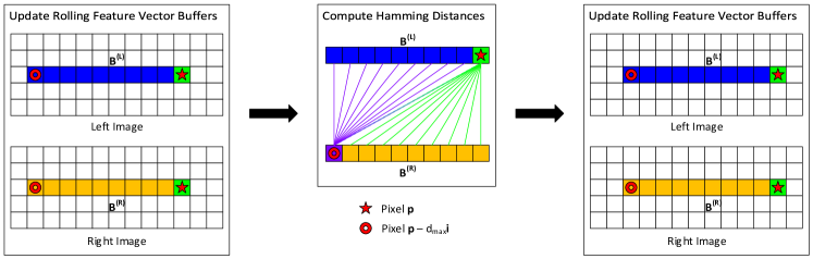
Figure 2: Computing the unaries: at each pixel $\mathbf{p}$, we compute $\phi^{(\mathcal{L})}(\mathbf{p})$ and $\phi^{(\mathcal{R})}(\mathbf{p})$ and use them to update the rolling buffers $B^{(\mathcal{L})}$ and $B^{(\mathcal{R})}$. We then compute the unaries $C_{\mathbf{p}}^{(\mathcal{L})}(d)$ and $C_{\mathbf{p}-d_{\max}\mathbf{i}}^{(\mathcal{R})}(d)$ for all $d\in\mathcal{D}$ as the Hamming distances between the relevant feature vectors (see Equation 10) before moving on to the next pixel.

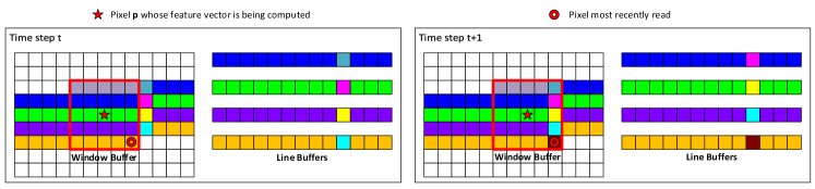
Figure 3: The buffers used to compute the Census Transform feature vectors, and how they are updated (see Section III-A1).

MGM [9] is effective at removing streaking, but since all but two of its directional minimisations (the purple and green ones in 1(c), for which $\mathbf{r}=[1,0]^{\top}$ and $\mathbf{r}=[1,-1]^{\top}$) rely on pixels that would be unavailable when streaming the image in raster order, a full FPGA implementation of the algorithm is difficult to achieve (see Section II-A1). One solution is to implement a cut-down MGM that only uses those of its directional minimisations that do work on an FPGA (i.e. the purple and green ones), mirroring one way in which SGM has been adapted for FPGA deployment [2]. However, if we limit ourselves to only one of MGM’s directional minimisations (e.g. the purple one), then the ‘region of influence’ of each pixel shrinks, resulting in poorer disparities, and if we use both, then we are forced to use double the amount of memory to store the cost vectors (see Section II-A1).

To avoid both problems, we propose a compromise, inspired by the way in which MGM allows each directional cost for a pixel to be influenced by neighbouring pixels in more than one direction to mitigate streaking. Our approach uses only a single directional minimisation, but one that incorporates information from all of the directions that are available when processing in raster order. This approach is inherently raster-friendly, and requires a minimal amount of memory on the FPGA. When processing the image in raster order, we compute the cost vector for each pixel by accumulating contributions from the $4$ of its $8$ neighbours that have already been visited and had their costs computed (the left, top-left, top and top-right neighbours, as per 1(d)). Formally, if we let

$$\footnotesize X=\left\{\rightarrow,\searrow,\downarrow,\swarrow\right\}=\left\{\left[\begin{array}[]{c}1\\ 0\end{array}\right],\left[\begin{array}[]{c}1\\ 1\end{array}\right],\left[\begin{array}[]{c}0\\ 1\end{array}\right],\left[\begin{array}[]{c}-1\\ 1\end{array}\right]\right\},$$ (8)

then we can compute the cost vector $L(\mathbf{p},\cdot)$ for pixel $\mathbf{p}$ via:

$$L(\mathbf{p},d)=C_{\mathbf{p}}(d)+\frac{1}{|X|}\sum_{\mathbf{x}\in X}\biggl{(} \min_{d^{\prime}\in\mathcal{D}}\left(L(\mathbf{p}-\mathbf{x},d^{\prime})+V(d,d^{\prime})\right)$$ (9)

$$- \min_{d^{\prime}\in\mathcal{D}}\left(L(\mathbf{p}-\mathbf{x},d^{\prime})\right)\biggr{)}$$

Since, unlike SGM and MGM, we only use a single minimisation, this is like Equation 5 in those approaches, letting us obtain each pixel’s cost vector in a single pass over the image.

In our implementation, we use the Census Transform (CT) [49] to compute the unaries $C_{\mathbf{p}}$. CT is robust to illumination changes between the images, and can be computed efficiently and in a raster-friendly way (see Section III-A1). Moreover, the Hamming distance between two CT feature vectors can be computed efficiently, and provides a good measure of their similarity. We compute the pixel costs $L(\mathbf{p},d)$ simultaneously for both the left and right images, thanks to our FPGA implementation (see Section III-A2). After selecting the best disparity in each image with a WTA approach, we process the disparities with a median filter (in a raster-friendly way) to reduce noise in the output. Finally, we validate our disparities with a standard LR check to discard inconsistent results [17], using a threshold of $1$ disparity or $3\%$, whichever is greater.

III-A FPGA Implementation

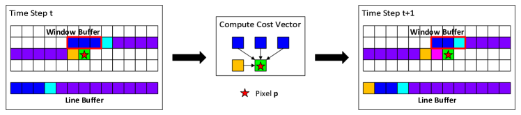
Figure 4: The buffers used to compute the cost vectors, and how they are updated (see Section III-A2).

Having described our approach conceptually, we now show how to implement it on an FPGA. By contrast to the previous sections, in which we only showed how to compute the disparities for pixels in the left image, here we describe how to compute the disparities for the pixels in both images efficiently to support LR consistency checking (see Section II-A). Notationally, we distinguish between the unary costs and cost vectors for the two images using the superscripts $(\mathcal{L})$ and $(\mathcal{R})$.

Two main steps are involved: (i) the computation of the unary costs $C_{\mathbf{p}}^{(\mathcal{L})}(\cdot)$ and $C_{\mathbf{p}}^{(\mathcal{R})}(\cdot)$, and (ii) the recursive computation of the cost vectors $L^{(\mathcal{L})}(\mathbf{p},\cdot)$ and $L^{(\mathcal{R})}(\mathbf{p},\cdot)$. Implementing these steps efficiently on an FPGA requires understanding the hardware, which essentially consists of a set of programmable logic blocks that can be wired together in different ways and independently programmed to perform different functions. This architecture naturally lends itself to an efficient pipeline-processing style, in which data is fed into the FPGA in a stream and different logic blocks try to operate on different pieces of data concurrently in each clock cycle. In practice, the steps we consider here all involve processing images, with the data associated with the images’ pixels being streamed into the FPGA in raster order, as we now describe.

III-A1 Unary Computation

Each unary $C_{\mathbf{p}}^{(\mathcal{L})}(d)$, which denotes the cost of assigning pixel $\mathbf{p}$ in the left image a disparity of $d$, is computed as the Hamming distance $\mathcal{H}$ between the feature vector $\phi^{(\mathcal{L})}(\mathbf{p})$ of pixel $\mathbf{p}$ in the left image and the feature vector $\phi^{(\mathcal{R})}(\mathbf{p}-d\mathbf{i})$ of pixel $\mathbf{p}-d\mathbf{i}$ in the right image. ($\phi^{(\mathcal{L})}(\mathbf{p})$ is computed by applying the Census Transform [49] to a $W\times W$ window around $\mathbf{p}$ in the left image, and analogously for $\phi^{(\mathcal{R})}$.) Conversely, $C_{\mathbf{p}}^{(\mathcal{R})}(d)$ becomes the Hamming distance between $\phi^{(\mathcal{R})}(\mathbf{p})$ and $\phi^{(\mathcal{L})}(\mathbf{p}+d\mathbf{i})$.

As per Figure 2, we traverse both the left and right images simultaneously in raster order, computing $\phi^{(\mathcal{L})}(\mathbf{p})$ and $\phi^{(\mathcal{R})}(\mathbf{p})$ for each pixel $\mathbf{p}$ as we go, and maintaining rolling buffers $B^{(\mathcal{L})}$ and $B^{(\mathcal{R})}$ of feature vectors for the most recent $d_{\max}+1$ pixels in each image, i.e. $B^{(\mathcal{L})}=[\phi^{(\mathcal{L})}(\mathbf{p}-d\mathbf{i}):d\in\mathcal{D}]$, and analogously for the right image. After computing the feature vectors for pixel $\mathbf{p}$, we compute unaries for all $d\in\mathcal{D}$:

$$C_{\mathbf{p}}^{(\mathcal{L})}(d) =\mathcal{H}(\phi^{(\mathcal{L})}(\mathbf{p}),\phi^{(\mathcal{R})}(\mathbf{p}-d\mathbf{i}))$$ (10)

$$C_{\mathbf{p}-d_{\max}\mathbf{i}}^{(\mathcal{R})}(d) =\mathcal{H}(\phi^{(\mathcal{L})}(\mathbf{p}+(d-d_{\max})\mathbf{i}),\phi^{(\mathcal{R})}(\mathbf{p}-d_{\max}\mathbf{i}))$$

Note that we compute the unaries for right image pixels just before they leave $B^{(\mathcal{R})}$, since it is only at that point that we have accumulated the feature vectors for all of the relevant left image pixels in $B^{(\mathcal{L})}$ (see Figure 2).

In practice, to efficiently compute the feature vectors, we must maintain a $W\times W$ window of the pixels surrounding $\mathbf{p}$ that can be used to compute the Census Transform [49]. As shown in Figure 3, we store this in a window buffer (local registers on an FPGA that can be used to store data to which we require instantaneous access). To keep the window buffer full, we must read ahead of $\mathbf{p}$ by slightly over $\lfloor W/2\rfloor$ rows. Separately, we maintain pixels from the rows above/below $\mathbf{p}$ in line buffers (regions of memory on an FPGA that can store larger amounts of data but can only provide a single value per clock cycle). As shown in Figure 3, some pixels are in both the window buffer and one of the line buffers. When moving from one pixel to the next, we update the window buffer and line buffers as shown in Figure 3. Notice how the individually marked pixels in the line buffers are shifted upwards to make way for the new, brown pixel that is being read in (to both the orange line buffer and the window buffer), and how the turquoise pixel is removed from the blue line buffer but added to the top-right of the window buffer. All of these operations can be implemented very efficiently on an FPGA.

III-A2 Cost Vector Computation

Once the unaries have been computed, the next step is to compute the $L(\mathbf{p},d)$ values (i.e. the cost vector) for each pixel using Equation 9. This again involves a walk over the image domain in raster order. In this case, computing the cost vector for each pixel $\mathbf{p}$ uses the cost vectors of the pixels $\mathbf{p}-\mathbf{x}$, for each $\mathbf{x}\in X$ (i.e. the $3$ pixels above $\mathbf{p}$ and the pixel to its left). As a result, these must be in memory when the cost vector for $\mathbf{p}$ is computed.

In practice, as shown in Figure 4, we divide the relevant cost vectors between several different locations in memory: (i) a line buffer whose size is equal to the width of the image, (ii) a window buffer that holds the cost vectors for the $3$ pixels above $\mathbf{p}$, and (iii) a register that holds the cost vector for the pixel to its left (the yellow pixel in Figure 4). This provides us with instantaneous access to the cost vectors that we need to compute the cost vector for $\mathbf{p}$, whilst keeping track of the cost vectors for the pixels that we will need to compute the cost vectors for upcoming pixels (via the line buffer). When moving from one pixel to the next, we update the window buffer and line buffer as shown in Figure 4. For the actual computation of $L(\mathbf{p},d)$, we rewrite Equation 9 as follows:

$$L(\mathbf{p},d)= \;C_{\mathbf{p}}(d)+\frac{1}{|X|}\sum_{\mathbf{x}\in X}\biggl{(}$$ (11)

$$\;\begin{aligned} \min{}\Bigl{\{}&L(\mathbf{p}-\mathbf{x},d),L(\mathbf{p}-\mathbf{x},d-1)+P_{1},\\ &L(\mathbf{p}-\mathbf{x},d+1)+P_{1},\min_{d^{\prime}\in\mathcal{D}}(L(\mathbf{p}-\mathbf{x},d^{\prime})+P_{2})\Bigr{\}}\\ \end{aligned}$$

$$- \min_{d^{\prime}\in\mathcal{D}}\left(L(\mathbf{p}-\mathbf{x},d^{\prime})\right)\biggr{)}$$

This allows for a more optimal implementation in which we store $\min_{d^{\prime}\in\mathcal{D}}(L(\mathbf{p}-\mathbf{x},d^{\prime})$ to avoid repeat computations.

Method	D1 Valid	Density	D1 Interpolated	Runtime	Environment	Power Consumption (W)
						(approx.)
Ours	4.8%	85.0%	9.9%	0.014s	FPGA (Xilinx ZC706)	3
DeepCostAggr [24]	–	99.98%	6.3%	0.03s	Nvidia GTX Titan X	250
CSCT+SGM+MF [15]	–	100%	8.2%	0.006s	Nvidia GTX Titan X	250

TABLE I: The quantitative results of our approach, in comparison to state-of-the-art GPU-based real-time methods, on the Stereo 2015 subset of the KITTI dataset [29, 30]. D1 Valid: error rate on the pixels surviving the LR check; Density: % of pixels output by the algorithm (in our case after the LR check); D1 Interpolated: error rate after interpolating according to the KITTI protocol. We use a threshold of $3$ disparity values or 5%, whichever is greater (i.e. the standard thresholds for KITTI). Our approach is able to produce post-interpolation results that are within striking distance of existing methods, whilst being two orders of magnitude more power-efficient and requiring much less computational power.

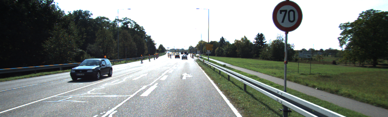
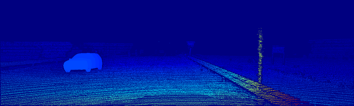
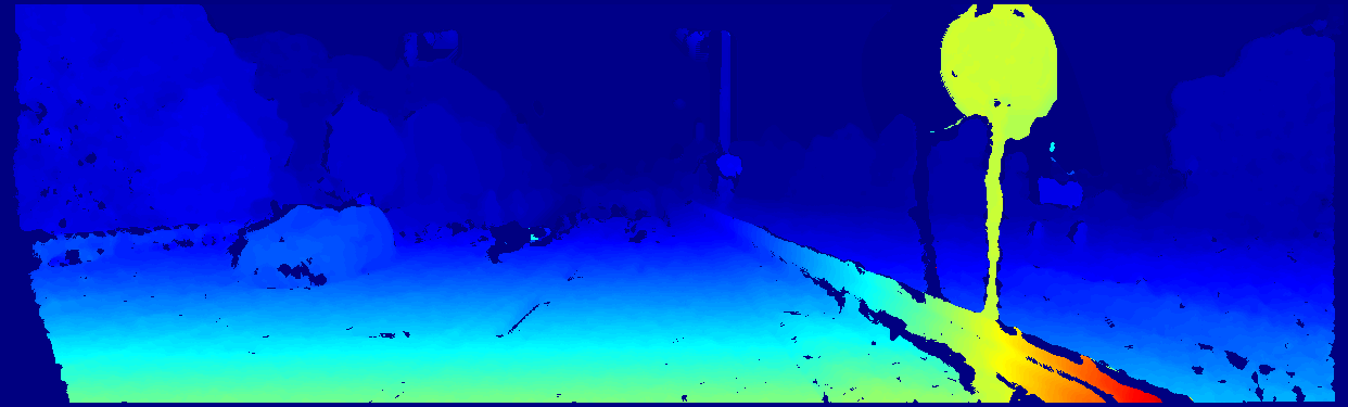
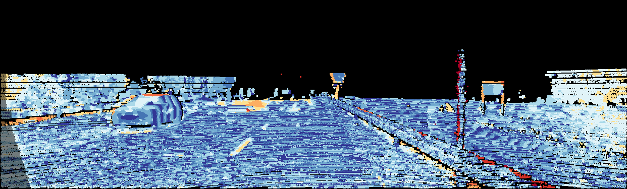
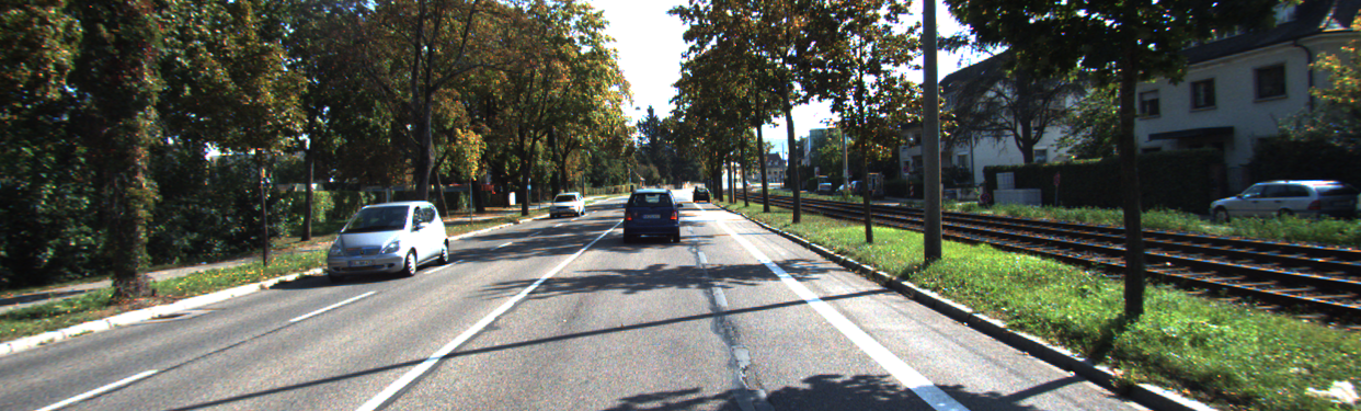
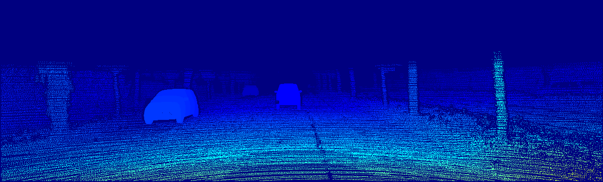
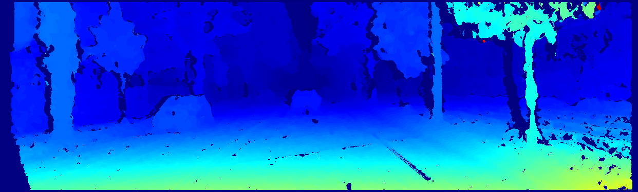
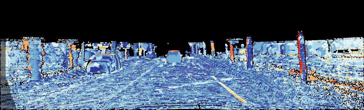
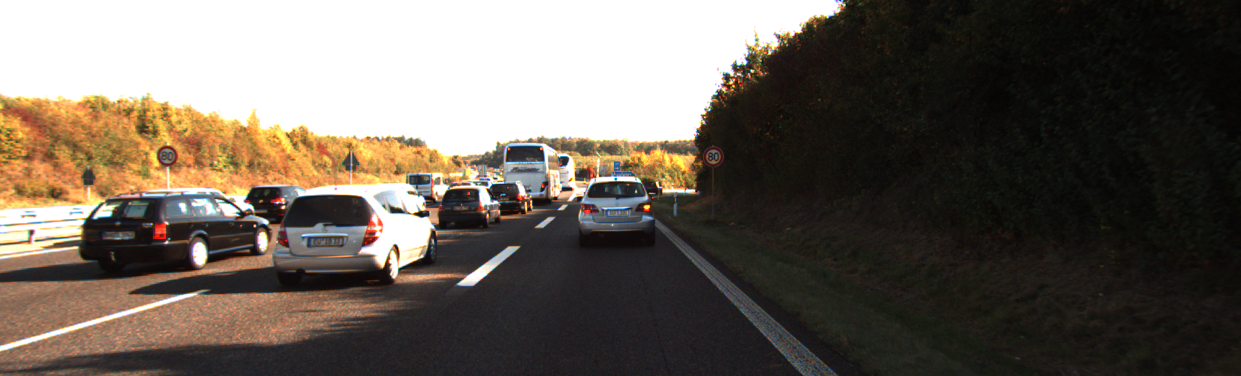
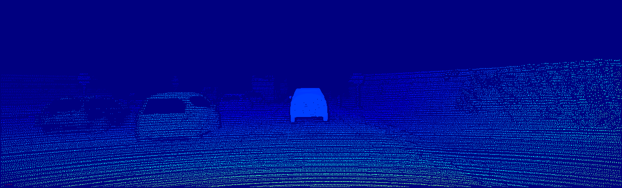
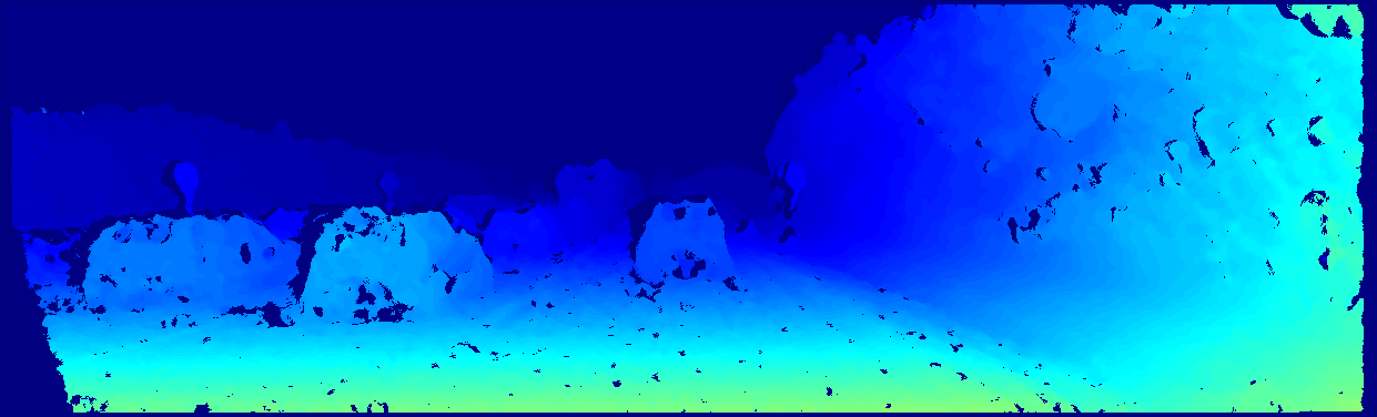
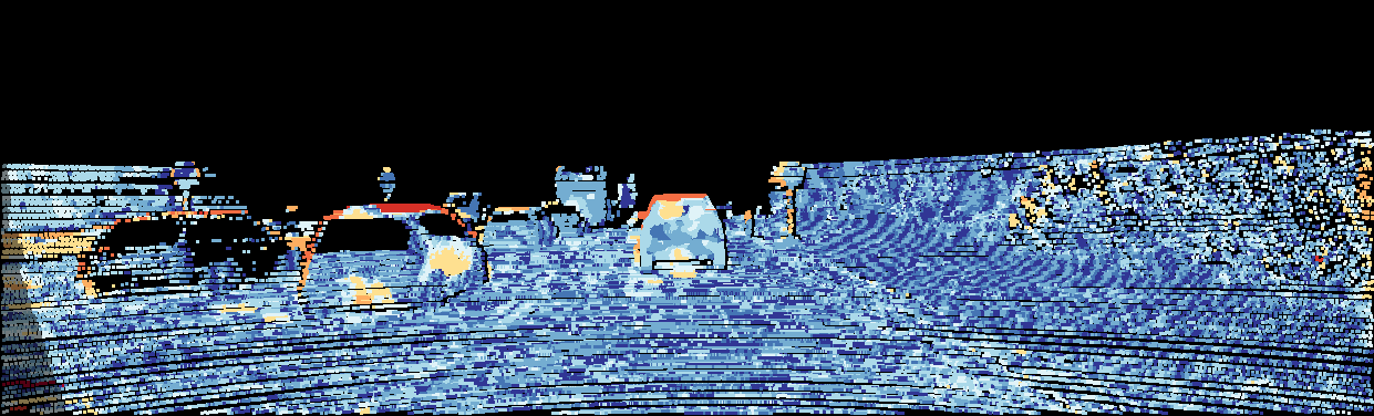
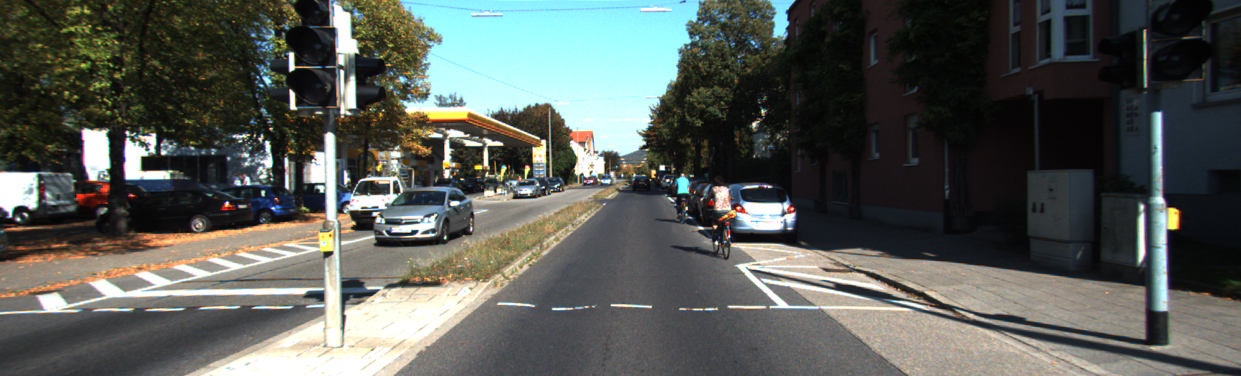
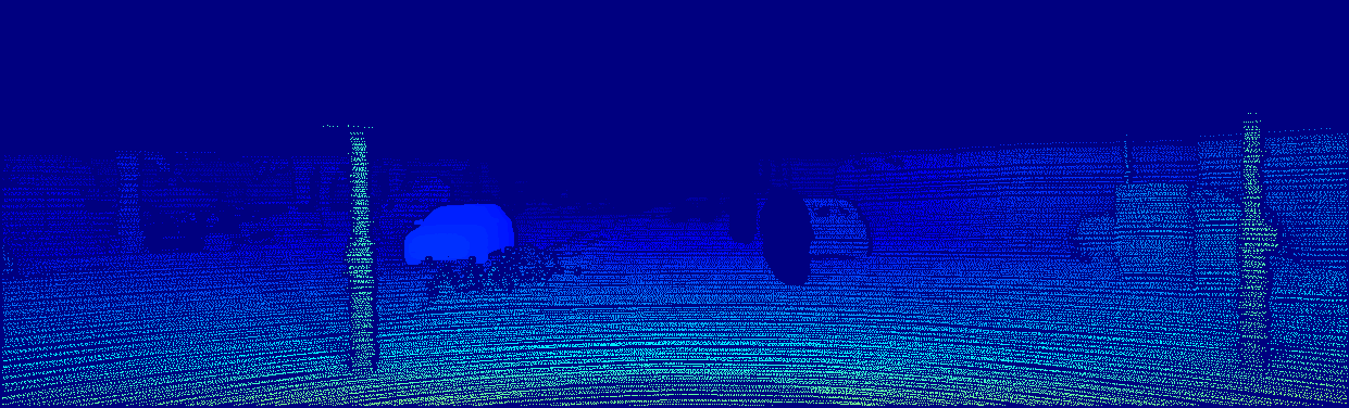
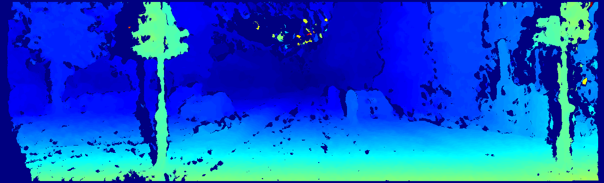
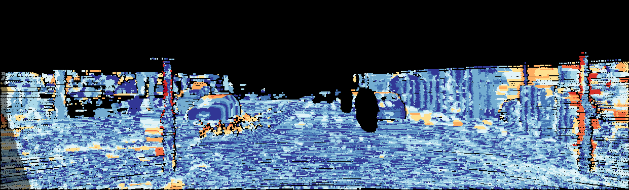
Figure 5: Qualitative examples of our approach on KITTI frames [29, 30]. Column 1: input left eye image; column 2: ground truth disparities; column 3: the disparities produced by our approach; column 4: error image (blue = low, red = high).

Method	Cones			Teddy			Tsukuba			Venus
	non-occ.	all	disc.	non-occ.	all	disc.	non-occ.	all	disc.	non-occ.	all	disc.
Ours	3.4	8.9	10.3	8.2	14.6	22.4	9.7	11.2	31.2	1.0	1.6	11.9
[2], 4 paths	9.5	–	–	13.3	–	–	6.8	–	–	4.1	–	–
[2], 8 paths	8.4	–	–	11.4	–	–	4.1	–	–	2.7	–	–
[10]	–	9.5	–	–	13.3	–	–	5.9	–	–	3.9	–
[42]	3.5	11.1	9.6	7.5	14.7	19.4	3.6	4.2	14.0	0.5	0.9	2.8
[46]	17.1	25.9	25.8	21.5	28.1	28.8	4.5	6.0	12.7	6.0	7.5	18.2
[50]	5.4	11.0	13.9	7.2	12.6	17.4	3.8	4.3	14.2	1.2	1.7	5.6
[34]	9.3	11.1	17.5	6.0	7.4	18.7	8.8	16.4	20.0	3.9	12.0	10.3

TABLE II: The accuracy of some FPGA-based methods on Middlebury images [39, 40]. The %’s are of pixels with a disparity error $>1$ pixel from ground truth: non-occ. = non-occluded pixels only, disc. = pixels near discontinuities only.

IV Experiments

We evaluate our approach on the KITTI [29, 30] and Middlebury [39, 40] datasets. We then compare our frame rate across different resolutions and disparity ranges vs. competing FPGA-based approaches. Finally, we break down the FPGA resource costs, associated power consumption, as well as accuracy of our approach for several variations of our design.

On KITTI, we compare our approach to the only two published approaches from the benchmark that are able to achieve state-of-the-art performance in real time [24, 15], both of which require a powerful GPU (an Nvidia GTX Titan X) to run. Since, unlike these approaches, our approach does not naturally produce disparities for every single pixel in the image, we interpolate as specified by the KITTI evaluation protocol in order to make our results comparable with theirs. As shown in Table I, we are able to achieve post-interpolation results that are competitive on accuracy with these approaches, whilst significantly reducing the power consumption and the compute power required. Furthermore, compared to the additional power efficient implementation reported in [15] (on a Nvidia Tegra X1), which achieves 13.8 fps with 10 Watts when scaled to the KITTI dataset, our system is more than five times faster, whilst consuming less than a third of the power. Moreover, we are able to achieve an even better error rate (4.8%) pre-interpolation, with a density of 85%. For some applications, this may in practice be more useful than having poorer disparities over the whole image. Qualitative examples of our approach on KITTI frames are shown in Figure 5.

On Middlebury, we show in Table II and Table III that we are able to achieve comparable accuracy to a number of other FPGA-based methods, whilst either running at a much higher frame-rate (c.f. [10, 46]), using simpler, cheaper hardware (c.f. [42]) or handling greater disparity ranges (c.f. [34, 50]). Figure 6 shows some examples of our approach on the four most commonly used Middlebury images, namely Cones, Teddy, Tsukuba and Venus.

Method	Resolution	Disparities	FPS	Environment
Ours	384x288	32	301	Xilinx ZC706
	450x375	64	198
	640x480	128	109
	1242x375	128	72
[2], 4 paths	640x480	64	66–167	Xilinx Virtex 5
	640x480	128	37–103
[10]	340x200	64	27	Xilinx Virtex 4
[28]	640x480	32	$\geq 30$	Xilinx Spartan 6 LX
[42]	352x288	64	1121	Altera Stratix IV
	640x480	64	357
	1024x768	128	129
	1920x1080	256	47.6
[46]	320x240	64	115	Xilinx Virtex 5
	320x240	128	66
	640x480	64	30
	800x600	64	19
[41]	1024x508	128	15	Xilinx Spartan 6
[20]	752x480	32	$\geq 60$	Xilinx Artix 7
[50]	1024x768	64	60	Altera EP3SL150
[34]	640x480	32	101	Xilinx Zynq-7000

TABLE III: The frame rates we can achieve, in comparison to those achieved by other FPGA-based methods, for multiple resolution/disparity range combinations.

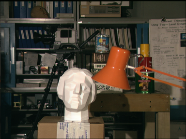
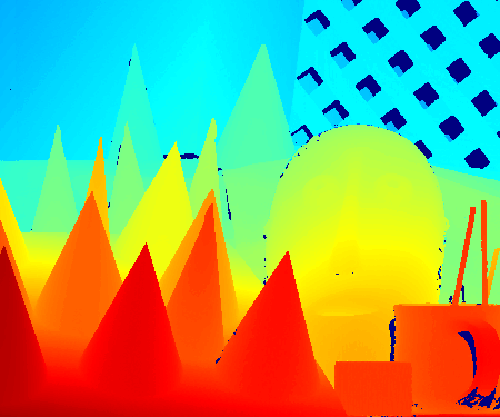
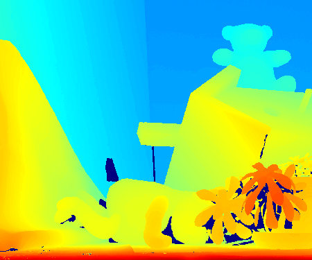
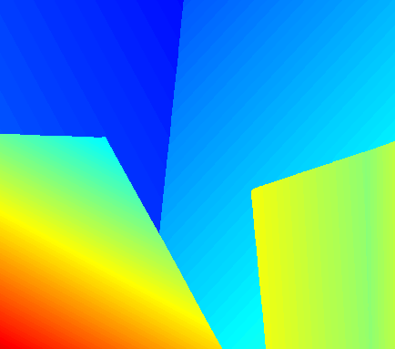
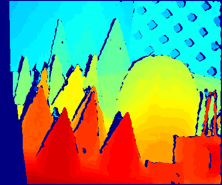
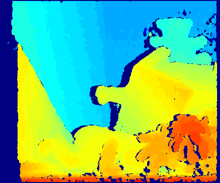
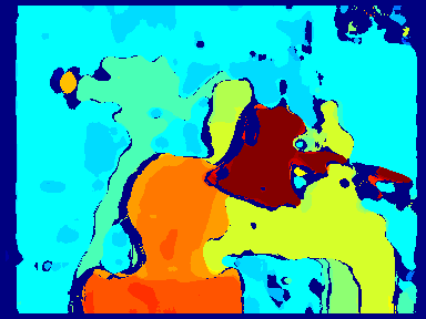
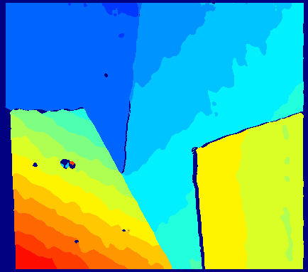
Figure 6: Our results on the four most commonly used Middlebury images [39, 40]. Left to right: Cones, Teddy, Tsukuba, Venus. Top row: input images; middle row: ground truth disparities; bottom row: the disparities produced by our approach.

The FPGA accelerators are designed and implemented through Xilinx’s High Level Synthesis (HLS) tool, whose C++ abstraction to FPGA development allows for faster prototyping during the design process, greater flexibility as well as improved reusability of the resulting hardware blocks. Through the use of Xilinx’s SDSoC tool, we deploy the accelerators on the ZC706 development board. In Table IV, we highlight how the frame rate of our system is independent of the window size of the Census Transform that we employ. Varying these parameter has, instead, an effect on the quality of the estimated disparities: as the window size increases, the error rate on the KITTI dataset images [29, 30] decreases. As in Table I, we report the error rate of the pixels surviving LR check (i.e. the output of the proposed method) together with their density, and the error rate after an interpolation step done according to the KITTI protocol. As expected, variations in the CT window size also affect the FPGA resource utilisation of the system, i.e. the number of logic/memory units that are required to implement the necessary hardware blocks. This resource utilisation, in turn, impacts the overall amount of power consumed by the FPGA chip, as estimated by the Xilinx Vivado tool. This is also shown, in the last row of Table IV. A justification for the frame-rates we achieve is that the embedded system manages to output one output disparity (for both left and right images) per three clock cycles (FPGA clocked at 100MHz). Although the system is fully pipelined, a strict dependency is incurred due to the use of the energy term of the previous pixel’s disparity result for the computation of the current pixel’s energy values, as denoted in Equation (11). More specifically, the system’s bottleneck and upper limit on frame-rate is due to the propagation delay required to compute the minimum of any given pixel’s cost vector.

V Conclusion

In this paper, we have presented R³SGM, a variant of the well-known Semi-Global Matching (SGM) method [17] for stereo disparity estimation that is better-suited to raster processing on an FPGA. We draw inspiration from the recent More Global Matching work of Facciolo et al. [9], which mitigated the streaking artifacts that afflict SGM by incorporating information from two directions into the costs associated with each scan line. Due to the memory access pattern involved in some of its directional minimisations, however, MGM proves difficult to efficiently accelerate. Instead, we propose a method that uses only a single, raster-friendly minimisation, but one that incorporates information from four directions at once.

Window Width	3	5	7	9	11	13
Frame Rate	72	72	72	72	72	72
Error %	9.3	6.7	5.8	5.4	5.0	4.8
Density %	73	81	83	84	85	85
Interp. Error %	19.4	13.6	12.0	11.1	10.5	9.9
LUT Utilisation %	33.4	37.6	49.9	58.3	67.3	75.7
FF Utilisation %	10.8	14.2	18.1	24.7	32.2	40.5
BRAM Utilisation %	28.9	29.3	29.6	30.0	30.4	30.7
Total FPGA Power (W)	1.68	1.85	2.02	2.36	3.52	3.94

TABLE IV: The impact of varying the Census Transform window size on the frame rate, error and FPGA resource utilisation. As the window size increases, the frame rate remains constant, the error on images from the KITTI dataset [29, 30] decreases, and the FPGA resource utilisation increases. Power consumption estimates were obtained from Xilinx Vivado.

Our approach compares favourably with the two state-of-the-art GPU-based methods [24, 15] that can process the KITTI dataset in real time, achieving similar levels of accuracy whilst reducing the power consumption by two orders of magnitude. Moreover, in comparison to other FPGA-based methods on the Middlebury dataset, we achieve comparable accuracy either at a much higher frame-rate (c.f. [10, 46]), using simpler, cheaper hardware (c.f. [42]) or handling greater disparity ranges (c.f. [34, 50]). Our approach achieves a state-of-the-art balance between accuracy, power efficiency and speed, making it particularly well suited to real-time applications that require low power consumption, such as prosthetic glasses and micro-UAVs.

References

- [1] J. Banks and P. Corke. Quantitative Evaluation of Matching Methods and Validity Measures for Stereo Vision. IJRR, 20(7):512–532, 2001.
- [2] C. Banz, S. Hesselbarth, H. Flatt, H. Blume, and P. Pirsch. Real-Time Stereo Vision System using Semi-Global Matching Disparity Estimation: Architecture and FPGA-Implementation. In SAMOS, pages 93–101, 2010.
- [3] F. Besse, C. Rother, A. Fitzgibbon, and J. Kautz. PMBP: PatchMatch Belief Propagation for Correspondence Field Estimation. IJCV, 110(1):2–13, 2014.
- [4] T. Cavallari, S. Golodetz*, N. A. Lord*, J. Valentin, L. D. Stefano, and P. H. S. Torr. On-the-Fly Adaptation of Regression Forests for Online Camera Relocalisation. In CVPR, pages 4457–4466, 2017.
- [5] Q. Chen and V. Koltun. Fast MRF Optimization with Application to Depth Reconstruction. In CVPR, pages 3914–3921, 2014.
- [6] G. Cocorullo, P. Corsonello, F. Frustaci, and S. Perri. An efficient hardware-oriented stereo matching algorithm. Microprocessors and Microsystems, 46:21–33, 2016.
- [7] L. De-Maeztu, S. Mattoccia, A. Villanueva, and R. Cabeza. Linear stereo matching. In ICCV, pages 1708–1715, 2011.
- [8] A. Drory, C. Haubold, S. Avidan, and F. A. Hamprecht. Semi-Global Matching: a principled derivation in terms of Message Passing. In GCPR, pages 43–53, 2014.
- [9] G. Facciolo, C. de Franchis, and E. Meinhardt. MGM: A Significantly More Global Matching for Stereovision. In BMVC, 2015.
- [10] S. K. Gehrig, F. Eberli, and T. Meyer. A Real-Time Low-Power Stereo Vision Engine Using Semi-Global Matching. In ICVS, pages 134–143, 2009.
- [11] A. Geiger, P. Lenz, and R. Urtasun. Are we ready for Autonomous Driving? The KITTI Vision Benchmark Suite. In CVPR, 2012.
- [12] C. Georgoulas and I. Andreadis. A real-time fuzzy hardware structure for disparity map computation. JRTIP, 6(4):257–273, 2011.
- [13] C. Godard, O. M. Aodha, and G. J. Brostow. Unsupervised Monocular Depth Estimation with Left-Right Consistency. In CVPR, 2017.
- [14] S. Golodetz∗, T. Cavallari∗, N. A. Lord∗, V. A. Prisacariu, D. W. Murray, and P. H. S. Torr. Collaborative Large-Scale Dense 3D Reconstruction with Online Inter-Agent Pose Optimisation. arXiv preprint arXiv:1801.08361, 2018.
- [15] D. Hernandez-Juarez, A. Chacón, A. Espinosa, D. Vázquez, J. C. Moure, and A. M. López. Embedded real-time stereo estimation via Semi-Global Matching on the GPU. Procedia Computer Science, 80, 2016.
- [16] S. L. Hicks, I. Wilson, L. Muhammed, J. Worsfold, S. M. Downes, and C. Kennard. A Depth-Based Head-Mounted Visual Display to Aid Navigation in Partially Sighted Individuals. PLoS ONE, 2013.
- [17] H. Hirschmuller. Stereo Processing by Semi-Global Matching and Mutual Information. T-PAMI, 30(2):328–341, 2008.
- [18] H. Hirschmüller. Semi-Global Matching – Motivation, Developments and Applications. Photogrammetric Week 11, pages 173–184, 2011.
- [19] H. Hirschmuller and D. Scharstein. Evaluation of stereo matching costs on images with radiometric differences. T-PAMI, 31(9), 2009.
- [20] D. Honegger, H. Oleynikova, and M. Pollefeys. Real-time and Low Latency Embedded Computer Vision Hardware Based on a Combination of FPGA and Mobile CPU. In IROS, pages 4930–4935, 2014.
- [21] A. Hosni, M. Bleyer, and M. Gelautz. Secrets of adaptive support weight techniques for local stereo matching. CVIU, 117(6):620–632, 2013.
- [22] A. Hosni, C. Rhemann, M. Bleyer, C. Rother, and M. Gelautz. Fast Cost-Volume Filtering for Visual Correspondence and Beyond. T-PAMI, 35(2):504–511, 2013.
- [23] N. Komodakis, G. Tziritas, and N. Paragios. Fast, Approximately Optimal Solutions for Single and Dynamic MRFs. In CVPR, 2007.
- [24] A. Kuzmin, D. Mikushin, and V. Lempitsky. End-to-end Learning of Cost-Volume Aggregation for Real-time Dense Stereo. In MLSP, pages 1–6, 2017.
- [25] K. Lai, L. Bo, X. Ren, and D. Fox. Rgb-d object recognition: Features, algorithms, and a large scale benchmark. In Consumer Depth Cameras for Computer Vision, pages 167–192. Springer, 2013.
- [26] Y. Li, K. Huang, and L. Claesen. SoC and FPGA Oriented High-quality Stereo Vision System. In FPL, pages 1–4, 2016.
- [27] F. Liu, C. Shen, G. Lin, and I. Reid. Learning Depth from Single Monocular Images Using Deep Convolutional Neural Fields. T-PAMI, 38(10):2024–2039, 2016.
- [28] S. Mattoccia and M. Poggi. A passive RGBD sensor for accurate and real-time depth sensing self-contained into an FPGA. In ICDSC, pages 146–151, 2015.
- [29] M. Menze and A. Geiger. Object Scene Flow for Autonomous Vehicles. In CVPR, pages 3061–3070, 2015.
- [30] M. Menze, C. Heipke, and A. Geiger. Joint 3D Estimation of Vehicles and Scene Flow. ISPRS Annals, 2:427, 2015.
- [31] H. Oleynikova, D. Honegger, and M. Pollefeys. Reactive avoidance using embedded stereo vision for mav flight. In ICRA, 2015.
- [32] M. Pérez-Patricio and A. Aguilar-González. FPGA implementation of an efficient similarity-based adaptive window algorithm for real-time stereo matching. JRTIP, pages 1–17, 2015.
- [33] M. Pérez-Patricio, A. Aguilar-González, M. Arias-Estrada, H.-R. Hernandez-de Leon, J.-L. Camas-Anzueto, and J. de Jesús Osuna-Coutiño. An FPGA stereo matching unit based on fuzzy logic. Microprocessors and Microsystems, 42:87–99, 2016.
- [34] S. Perri, F. Frustaci, F. Spagnolo, and P. Corsonello. Stereo vision architecture for heterogeneous systems-on-chip. JRTIP, pages 1–23, 2018.
- [35] V. A. Prisacariu, O. Kähler, S. Golodetz, M. Sapienza, T. Cavallari, P. H. S. Torr, and D. W. Murray. InfiniTAM v3: A Framework for Large-Scale 3D Reconstruction with Loop Closure. arXiv preprint arXiv:1708.00783v1, 2017.
- [36] O. Rahnama, D. Frost, O. Miksik, and P. H. Torr. Real-Time Dense Stereo Matching With ELAS on FPGA-Accelerated Embedded Devices. RA-L, 3(3):2008–2015, 2018.
- [37] O. Rahnama, A. Makarov, and P. H. S. Torr. Real-Time Depth Processing for Embedded Platforms. In Proceedings of the SPIE, 2017.
- [38] D. Scharstein, H. Hirschmüller, Y. Kitajima, G. Krathwohl, N. Nešić, X. Wang, and P. Westling. High-Resolution Stereo Datasets with Subpixel-Accurate Ground Truth. In GCPR, pages 31–42, 2014.
- [39] D. Scharstein and R. Szeliski. A Taxonomy and Evaluation of Dense Two-Frame Stereo Correspondence Algorithms. IJCV, 47(1-3):7–42, 2002.
- [40] D. Scharstein and R. Szeliski. High-Accuracy Stereo Depth Maps Using Structured Light. In CVPR, 2003.
- [41] K. Schmid and H. Hirschmüller. Stereo Vision and IMU based Real-Time Ego-Motion and Depth Image Computation on a Handheld Device. In ICRA, pages 4671–4678, 2013.
- [42] Y. Shan, Y. Hao, W. Wang, Y. Wang, X. Chen, H. Yang, and W. Luk. Hardware Acceleration for an Accurate Stereo Vision System Using Mini-Census Adaptive Support Region. TECS, 13(4s), 2014.
- [43] J. Shotton, B. Glocker, C. Zach, S. Izadi, A. Criminisi, and A. Fitzgibbon. Scene Coordinate Regression Forests for Camera Relocalization in RGB-D Images. In CVPR, pages 2930–2937, 2013.
- [44] J. Sun, N.-N. Zheng, and H.-Y. Shum. Stereo Matching Using Belief Propagation. T-PAMI, 25(7):787–800, 2003.
- [45] K. Tateno, F. Tombari, I. Laina, and N. Navab. CNN-SLAM: Real-time dense monocular SLAM with learned depth prediction. In CVPR, pages 6243–6252, 2017.
- [46] C. Ttofis and T. Theocharides. Towards Accurate Hardware Stereo Correspondence: A Real-Time FPGA Implementation of a Segmentation-Based Adaptive Support Weight Algorithm. In DATE, 2012.
- [47] W. Wang, J. Yan, N. Xu, Y. Wang, and F.-H. Hsu. Real-Time High-Quality Stereo Vision System in FPGA. T-CSVT, 25(10), 2015.
- [48] M. Werner, B. Stabernack, and C. Riechert. Hardware Implementation of a Full HD Real-time Disparity Estimation Algorithm. T-CE, 60(1):66–73, 2014.
- [49] R. Zabih and J. Woodfill. Non-parametric Local Transforms for Computing Visual Correspondence. In ECCV, 1994.
- [50] L. Zhang, K. Zhang, T. S. Chang, G. Lafruit, G. K. Kuzmanov, and D. Verkest. Real-Time High-Definition Stereo Matching on FPGA. In FPGA, pages 55–64, 2011.
- [51] Z. Zhang. Microsoft Kinect Sensor and Its Effect. IEEE Multimedia, 19(2):4–10, 2012.