The Robustness of Cosmological Hydrodynamic Simulation Predictions to Changes in Numerics and Cooling Physics

Abstract

We test and improve the numerical schemes in our smoothed particle hydrodynamics (SPH) code for cosmological simulations, including the pressure-entropy formulation (PESPH), a time-dependent artificial viscosity, a refined timestep criterion, and metal-line cooling that accounts for photoionisation in the presence of a recently refined Haardt & Madau (2012) model of the ionising background. The PESPH algorithm effectively removes the artificial surface tension present in the traditional SPH formulation, and in our test simulations it produces better qualitative agreement with mesh-code results for Kelvin-Helmholtz instability and cold cloud disruption. Using a set of cosmological simulations, we examine many of the quantities we have studied in previous work. Results for galaxy stellar and HI mass functions, star formation histories, galaxy scaling relations, and statistics of the Ly$\alpha$ forest are robust to the changes in numerics and microphysics. As in our previous simulations, cold gas accretion dominates the growth of high-redshift galaxies and of low mass galaxies at low redshift, and recycling of winds dominates the growth of massive galaxies at low redshift. However, the PESPH simulation removes spurious cold clumps seen in our earlier simulations, and the accretion rate of hot gas increases by up to an order of magnitude at some redshifts. The new numerical model also influences the distribution of metals among gas phases, leading to considerable differences in the statistics of some metal absorption lines, most notably NeVIII.

1 INTRODUCTION

Numerical simulations are indispensable for our understanding of galaxy formation and evolution. In the $\mathrm{\Lambda CDM}$ model, dark matter haloes over a wide mass range form and grow through gravitational instability. Star formation and galaxy assembly take place within these gravitational potentials, where baryonic processes such as gas accretion, shock heating, and cooling are essential. Modelling these baryonic processes accurately is thus crucial. Cosmological simulations with simplified treatments of baryonic physics such as radiative cooling and photoionisation (Katz et al., 1996), star formation (Springel & Hernquist, 2003), chemical enrichment, and supernova feedback (e.g., Oppenheimer & Davé, 2006) have enjoyed many successes matching observational results on various spatial and time scales (Hernquist et al., 1996; Davé & Tripp, 2001; Governato et al., 2007; Oppenheimer & Davé, 2006, 2008; Davé et al., 2013). To make simulations faithfully represent the true universe, we need not only realistic prescriptions for the sub-grid physics, but also accurate and stable hydrodynamic solvers so that the simulated gas thermodynamics accurately converges to the behaviour of gas in the real physical world.

The two basic methods that evolve hydrodynamical systems are Eulerian based and Lagrangian based, which differ in how the fluid equations are discretised. The smoothed particle hydrodynamics (SPH) technique (Gingold & Monaghan, 1977; Lucy, 1977; Monaghan, 1992) discretises the fluid elements into particles that carry local thermodynamic quantities that are evaluated using kernel smoothing. The equations that govern the motion of SPH particles are derived rigorously from the discretised Lagrangian, automatically satisfying the continuity equation, and are symmetrised to guarantee a simultaneous conservation of energy, momentum and entropy (Springel & Hernquist, 2002). The pseudo-Lagrangian nature of SPH allows it to probe a large dynamic range in the cosmological context, and makes it convenient in studying accretion events and outflow models. Also, the particle based hydro-force calculation enables a straightforward coupling with many efficient algorithms for the gravity force calculation. However, SPH techniques have well-known weaknesses including poor shock resolution, over-damping of weak non-convergent velocity fields, and suppression of fluid instabilities. Mesh based codes solve the Eulerian hydrodynamical equations on a grid that divides the simulation volume. A weakness of grid-based codes is the lack of spatial dynamic range needed for a representative size of the universe. Adaptive mesh refinement (AMR) codes (Berger & Colella, 1989; Teyssier, 2002; Bryan et al., 2014) are designed to alleviate this problem, but still have other problems such as over mixing, not being Galiliean invariant, and poor coupling to gravity solvers (Vogelsberger et al., 2012; Hopkins, 2015). Some more recently developed algorithms, such as the moving mesh code AREPO (Springel, 2010b) or the Lagrangian volume method implemented in GIZMO (Hopkins, 2015), attempt to take advantage of the best properties of SPH and AMR. Assessing the relative merits of these schemes versus the overall class of SPH methods is a long-term project and one we will not address here.

The two classes of methods can give very different results in both standard test problems and cosmological simulations (Frenk et al., 1999; Hu et al., 2014; Sembolini et al., 2016a, b), and the disagreements are not alleviated by simply increasing the resolution (Agertz et al., 2007). In sub-sonic regimes, traditional SPH is believed to lead to unphysical results especially in regions where two fluids of strong density contrast intersect. The poor behaviour of SPH at fluid interfaces has been attributed to an erroneous pressure force analogous to a surface tension, which is caused by multi-valued pressures at contact discontinuities. Many modifications to traditional SPH have been proposed to alleviate this problem (Abel, 2011; Price, 2012; Read & Hayfield, 2012). However, these methods have certain problems such as increased run time, and a requirement for high order smoothing kernels that need a large number of neighbouring particles to keep an equivalent resolution. Furthermore, some methods introduced additional terms that violate the conservation properties of SPH (Peeples, 2010).

Saitoh & Makino (2013) pointed out that by using an alternative definition of the SPH volume element, a new set of equations can be derived to eliminate the surface tension term. Following their work, Hopkins (2013) derived a class of alternative SPH equations of motion from the discrete Lagrangian. His work shows that, without losing general conservation properties, this pressure-entropy formalism of SPH (referred to below as PESPH) makes significant improvements to the code’s performance at contact discontinuities. His tests show that the improvements are largely attributed to the optimal choice of hydrodynamical equations while the assumptions on smoothing kernel and artificial viscosity only have sub-dominant effects. Further improvements are realised if one also includes artificial conduction.

Another problematic aspect of SPH is the artificial viscosity. Owing to the entropy conserved nature of the Lagrangian fluid equations, an extra artificial viscosity term has to the added to the momentum equation of SPH to efficiently convert kinetic energy into thermal energy in shock regions. Usually the artificial viscosity needs to be much larger than the physical viscosity to avoid particle penetration between SPH particles in strong shocks. The traditional treatment of artificial viscosity (Springel, 2005), however, usually leads to a fluid that is too viscous, in which small velocity perturbations away from shocks are over damped. Therefore, a modified treatment of artificial viscosity that reduces unwanted dissipation in shock-free regions is motivated. Morris & Monaghan (1997) (hereafter M&M97) proposed a time-dependent method that adjusts the viscosity by a pre-factor that depends on the strength of the local convergent flow. Cullen & Dehnen (2010) presented a more complicated method that produces more accurate results in certain test problems, but the behaviour of their method in a cosmological context is still uncertain.

Meanwhile, a long standing problem in current galaxy formation theory is that cosmological simulations without external feedback processes have produced too many stars compared to observations (Kereš et al., 2005, 2009a). Recently, various forms of feedback have been adopted in studies of galaxy formation to suppress star formation. However, as pointed out by several authors (Saitoh & Makino, 2009; Merlin et al., 2010), the traditional timestep criterion is inaccurate in handling strong perturbations that arise from feedback prescriptions, leading to violations of energy conservation. Therefore, a SPH code using adaptive timesteps must ensure a prompt response of the system to strong energy perturbations from such feedback. Durier & Dalla Vecchia (2012) proposed a timestep limiter to address this problem for both thermal and kinetic feedback and demonstrated its success in standard tests such as the Sedov blast wave problem. They found that without properly limiting the timesteps errors can be as large as orders of magnitude.

Almost all of the above mentioned problems, solutions and tests have been performed on idealised problems that may or may not be important to simulations of galaxy formation. Furthermore, most of the tests are run at resolutions that are much higher than that usually obtained in galaxy formation simulations, whether in zoom-in simulations (Katz & White, 1993; Governato et al., 2007; Guedes et al., 2011; Hopkins et al., 2014) or in cosmological volumes (Vogelsberger et al., 2014; Schaye et al., 2015; Davé et al., 2016). In addition, choices in feedback algorithms may dominate over differences that result from the choice of hydrodynamics solver (Scannapieco et al., 2012; Schaller et al., 2015; Sembolini et al., 2016b).

To study the effects of these numerics in more realistic situations, in this work we run a series of simulations using the GADGET-3 code, which is an updated version of the widely used code GADGET-2 (Springel, 2005). It is a hybrid Tree-PM SPH code that aims at studies of gas dynamics within a gravitational background. The long range gravitational forces are evaluated using a particle mesh (PM) method (Hockney & Eastwood, 1981) and the short range forces are evaluated with an oct-tree algorithm (Barnes & Hut, 1986). The SPH in the original GADGET-3 uses the old density-entropy formalism (Springel & Hernquist, 2002), which manifestly conserves energy and entropy, but we have replaced the density-entropy SPH equations (referred to below as DESPH) with the new pressure-entropy SPH equations.

In our previous hydrodynamical cosmological simulations, we compute the metal-line cooling rate with the assumption of collisional ionisation equilibrium (CIE). The CIE assumption is, however, not rigorous since photoionisation reduces the amount of bound electrons and thus affects the cooling rates. Wiersma et al. (2009) computed non-CIE cooling rates in the presence of a radiative background and showed that photoionisation could suppress cooling in shocked gas by an order of magnitude. Furthermore, Haardt & Madau (2012) (HM12) published a more up-to-date estimate of the UV background flux with a more careful assessment of the galaxy and quasar contributions as a function of time. The effects of these recent updates in the sub-resolution physical models has yet to be studied in a cosmological context.

The main goal of this paper is to examine the impact of the new numerical treatments of hydrodynamics as well as the adopted prescriptions for the baryonic physics in a full cosmological simulation. We also perform standard tests to demonstrate the improvements made by the new SPH formalism. The simplified physics in the standard tests help us to understand the behaviour of different codes as one changes the numerical resolution. Since the relevant physics such as contact discontinuities, fluid instabilities, and mixing are prevalent in cosmic baryonic processes, such knowledge is important to interpreting the predictions of the baryons in the realistic yet much more complex problems of structure formation and evolution. We have published many predictions using DESPH with the old viscosity, cooling and UV background (Oppenheimer & Davé, 2006; Finlator & Davé, 2008; Oppenheimer & Davé, 2008; Oppenheimer et al., 2010; Davé et al., 2010; Peeples et al., 2010a, b; Davé et al., 2011a, b; Oppenheimer et al., 2012; Davé et al., 2013; Ford et al., 2013; Kollmeier et al., 2014; Ford et al., 2016), and would like to show which of those predictions are robust to these numerical and physical changes and which have been altered. This retrospective comparison is a necessary prelude to our future work using the new SPH code.

Schaller et al. (2015) compare a subset of EAGLE cosmological simulations that use traditional SPH and fiducial ANARCHY flavour of SPH, which includes the PESPH formulation, a simplified Cullen & Dehnen (2010) viscosity, artificial conduction and the timestep limiter. They conclude that the numerical improvements included in the ANARCHY SPH do not have significant effect on the properties of most galaxies. However, they use a thermal feedback scheme which is very different from our kinetic feedback scheme. The differences in the feedback model could result in very different gas properties in the universe that are likely to be sensitive to the numerical techniques. Therefore, our work is an independent test of the importance of numerics on the outcomes of cosmological simulations.

The paper is organised as follows. §2 describes our improvements to our numerical algorithms, including the new PESPH formulation, the artificial viscosity, artificial conduction, the timestep limiter, and the implementation of these changes into our cosmological code. We perform standard fluid dynamics tests with our updated code, and present the results in §3. We describe our cosmological tests - the subgrid physics, the simulation parameters, etc. in §4. In §5 we compare baryonic statistics such as stellar mass - halo mass relations, hot baryon fractions, baryonic accretion histories and the stellar mass functions, which result from our cosmological simulations, and in §6 we focus on comparing the properties of the intergalactic and circumgalactic medium, including Ly$\alpha$ statistics, metal line absorption lines. In all these comparisons we focus on the predictions that are the most sensitive to change, in both the numerics and physics. We present a summary in §7. In the Appendix we present results for those predictions that are not much affected by changes in the numerics and physics, and some additional idealised tests.

2 THE NEW HYDRODYNAMICS

2.1 A new hydro-solver

A comprehensive review of the standard SPH formalism can be found in Springel (2010a). The SPH equations of motion are derived from the Lagrangian form of the fluid equations. Each SPH particle represents a fluid element of small volume $\Delta V_{i}$, which defines the size of the smoothing kernel and connects the thermodynamic quantities, e.g., pressure and specific entropy. In traditional DESPH, the volume element is always assumed to be $m_{i}/\rho_{i}$, in which the density of the particle $\rho_{i}$ is computed by kernel averaging over its $N_{ngb}$ neighbouring particles, and $m_{i}$ is the mass of the particle. Hopkins (2013) highlights the freedom in the choice of this volume element without violating the conservation properties. A general way of defining the volume element can be written as the ratio of a particle-carried scalar value $x_{i}$ and its kernel averaged value $y_{i}$:

$$\Delta V_{i}=\frac{x_{i}}{y_{i}}$$ (1)

$$y_{i}\equiv\sum_{j=1}^{N_{ngb}}x_{i}W_{ij}(h_{i})$$ (2)

where $W_{ij}(h_{i})$ is the smoothing kernel for particle i. Springel & Hernquist (2002) found that the SPH equations derived from the discrete particle Lagrangian are able to conserve energy, momentum and entropy simultaneously if the smoothing length $h_{i}$ of each particle satisfies the constraint equation with a constant $N_{ngb}$ for all particles:

$$\Delta\tilde{V}=\frac{4\pi}{3}h_{i}^{3}\frac{1}{N_{ngb}}$$ (3)

The two volume elements, $\Delta V$ and $\Delta\tilde{V}$, defined through equation 1 and equation 3, respectively, do not have to be the same in a simulation. By taking into account the arbitrariness of the volume element choices, Hopkins (2013) derived the general form of the equations of motion (EoM):

$$m_{i}\frac{d\mathbf{v_{i}}}{dt}=-\sum_{j=1}^{N_{ngb}}x_{i}x_{j}\left[\frac{P_{i}}{y_{i}^{2}}f_{ij}\nabla_{i}W_{ij}(h_{i})+\frac{P_{j}}{y_{j}^{2}}f_{ji}\nabla_{i}W_{ij}(h_{j})\right]$$ (4)

$$f_{ij}\equiv 1-\frac{\tilde{x_{j}}}{x_{j}}\left(\frac{h_{i}}{3\tilde{y_{i}}}\frac{\partial{y_{i}}}{\partial{h_{i}}}\right)\left[1+\frac{h_{i}}{3\tilde{y_{i}}}\frac{\partial{\tilde{y_{i}}}}{\partial{h_{i}}}\right]^{-1}$$ (5)

where $\mathbf{v_{i}}$ is the velocity and $P_{i}$, $P_{j}$ are the pressure, $\tilde{x_{i}}$ and $\tilde{y_{i}}$ are associated with the volume $\Delta\tilde{V_{i}}$ that is defined through the constraint equation 3. The equations of motion for traditional SPH (DESPH) are recovered when the volume elements are defined as $x_{i}=\tilde{x_{i}}=m_{i}$, and $y_{i}=\tilde{y_{i}}=\rho_{i}$. However, Hopkins (2013) suggests an alternative choice, the pressure-entropy formulation: $x_{i}=m_{i}A_{i}^{1/\gamma},\tilde{x_{i}}=1(\Delta\tilde{V}=1/n_{i})$. In this formulation, which we refer to below as pressure-entropy SPH (PESPH), the quantity that is evaluated from direct kernel smoothing is now the pressure instead of the density:

$$P_{i}=y_{i}^{\gamma}=\left[\sum_{j=1}^{N_{ngb}}m_{j}A_{j}^{1/\gamma}W_{ij}(h_{i})\right]^{\gamma}$$ (6)

where $A_{j}$ is the specific entropy. With these choices the equations of motion become:

$$m_{i}\frac{\mathbf{v_{i}}}{dt}=-\sum_{j=1}^{N_{ngb}} m_{j}\left[\left(\frac{A_{j}}{A_{i}}\right)^{\frac{1}{\gamma}}+f_{i}\right]\left(\frac{A_{i}}{P_{i}}\right)^{\frac{2}{\gamma}}P_{i}\nabla_{i}W_{ij}(h_{i})+$$ (7)

$$m_{j}\left[\left(\frac{A_{i}}{A_{j}}\right)^{\frac{1}{\gamma}}+f_{j}\right]\left(\frac{A_{j}}{P_{j}}\right)^{\frac{2}{\gamma}}P_{j}\nabla_{i}W_{ij}(h_{j})$$ (8)

where,

$$f_{i}=\frac{h_{i}}{3A_{i}^{1/\gamma}m_{i}n_{i}}+\frac{\partial{P_{i}}^{1/\gamma}}{\partial{h_{i}}}\left[1+\frac{h_{i}}{3n_{i}}\frac{\partial{n_{i}}}{\partial{h_{i}}}\right]^{-1}$$ (9)

The density, now derived from the pressure, resembles an entropy weighted kernel average rather than a direct smoothing over its neighbouring particles:

$$u\equiv\frac{P_{i}}{(\gamma-1)\rho_{i}}=\frac{A_{i}\rho_{i}^{\gamma-1}}{\gamma-1}$$ (10)

where $u$ is the specific energy.

2.2 Kernel choice

The equations of motion allow for an arbitrary choice of the smoothing kernel $W_{ij}(r_{ij},h_{i})$. A standard cubic spline kernel with 32 neighbouring particles ($N_{ngb}=32$) has been adopted in our previous work, which used the DESPH formulation (e.g., Oppenheimer & Davé, 2006; Ford et al., 2016).

In recent years, high resolution standard tests demonstrate that different kernels can have a significant impact on certain problems, so the choice is not trivial. SPH suffers from an intrinsic $O(h^{-1})$ error in the momentum equation (Morris, 1996). This error can be reduced by increasing the number of neighbours, but without a proper choice for the kernel function numerical instabilities grow and degrade the results (Read et al., 2010; Dehnen & Aly, 2012). These authors consistently demonstrated that a higher-order kernel smoothing over a sufficient number of neighbours provides an effective solution in suppressing the errors and numerical instabilities. Following Hopkins (2013), we choose the quintic spline kernel with $N_{ngb}=128$ as our default, which has an effective resolution equal to a cubic spline kernel with 34 neighbours. This choice is motivated by test results from Hongbin & Xin (2005) and Dehnen & Aly (2012).

2.3 Artificial viscosity

SPH equations are intrinsically dissipationless in the sense that the entropy of each particle is conserved when there is no external heat or cooling source. To capture shocks in real physical situations, an artificial viscosity is added as a dissipation that converts the kinetic energy into thermal energy for gas particles in a converging flow. Traditionally a viscosity force is added to the momentum equation (Springel & Hernquist, 2003):

$$\frac{d\mathbf{v_{i}}}{dt}|_{visc}=-\sum_{j=1}^{N}m_{j}\Pi_{ij}\nabla_{i}\bar{W}_{ij}$$ (11)

where,

$$\Pi_{ij}=-\frac{\alpha}{2}\frac{(c_{i}+c_{j}-w_{ij})w_{ij}}{\rho_{ij}}$$ (12)

where $c_{i}$ and $c_{j}$ are the sound speed of particle i and j, respectively, $\rho_{ij}$ is the mean of their densities, and $w_{ij}=\mathbf{v_{ij}}\cdot\mathbf{r_{ij}}/|\mathbf{r_{ij}}|$ whenever particles are approaching each other ($\mathbf{v_{ij}}\cdot\mathbf{r_{ij}}>0$), otherwise $w_{ij}$ is set to 0 making for no viscous force. It is important to always convert comoving coordinates to physical ones whenever applying any artificial viscosity scheme.

The parameter $\alpha$ that appears in the above equation regulates the overall strength of the viscous force. It used to be empirically set to a constant value ($\alpha=0.2$ in our previous simulations). However, the standard artificial viscosity often leads to unnecessary damping of velocity perturbations in regions where turbulence dominates, because it only requires velocity convergence on a particle by particle basis. Morris & Monaghan (1997) proposed that the $\alpha$ parameter of each individual particle be allowed to vary depending on the local convergence of the flow. The $\alpha$ is adapted to evolve through the differential equation:

$$\dot{\alpha}=(\alpha_{min}-\alpha_{i})/\tau_{i}+S_{i}$$ (13)

The decay time-scale, $\tau_{i}$ is related to the sound crossing time and the source term $S_{i}$ is based on the local divergence of the velocity:

$$\tau_{i}=h_{i}/(2lc_{i})$$ (14)

$$S_{i}=S_{0}\times max\{-\nabla\cdot\mathbf{v_{i}},0\}$$ (15)

In our simulations that adopt the M&M viscosity, we set the parameters to $l=3.73,\alpha_{min}=0.1$, and $S_{0}=2.0$. We also imposed an upper limit of $\alpha_{max}=2.0$, preventing the viscosity from becoming too large owing to numerical noise. We also adopt the Balsara (1995) switch that aims to suppress viscosity in shear flows in conjunction with the Morris & Monaghan (1997) viscosity.

For a cosmological simulation in a co-moving volume, we add the Hubble flow of $3H(a)$ to the divergence to account for the expansion of the universe. In practise, when we use the new M&M viscosity in a cosmological simulation, the $\alpha$’s of the majority of the gas particles are kept at the lower limit of 0.1, retaining the turbulent nature of most of the diffuse gas. When a shock occurs, it is captured by the convergence check and the $\alpha$’s of shocked particles are boosted to a higher value compared to the traditional scheme, efficiently converting the shock energy into thermal energy. In the post-shock region, the $\alpha$’s decay back to the lower limit on a sound-crossing time-scale, which avoids further damping of the velocity perturbations.

Cullen & Dehnen (2010) recently provided an improved prescription for artificial viscosity and also a more accurate estimator for $\nabla\cdot\mathbf{v}$. In their method, a converging flow is predicted by a shock indicator that depends on the time derivative of the velocity divergence.

$$A_{i}=\xi_{i}max\left(-\dot{\nabla}\cdot\mathbf{v_{i}},0\right)$$ (16)

Here, $\xi_{i}$ is a limiter similar to the Balsara switch, which suppresses dissipation in shear flows:

$$\xi_{i}=\frac{\left|2(1-R_{i})^{4}\nabla\cdot\mathbf{v_{i}}\right|^{2}}{\left|2(1-R_{i})^{4}\nabla\cdot\mathbf{v_{i}}\right|^{2}+tr(\mathbf{S_{i}}\cdot\mathbf{S_{i}^{t}})}$$ (17)

where $\mathbf{S_{i}}$ is a traceless symmetric matrix defined in Cullen & Dehnen (2010) as an alternative to $\left|\nabla\times\mathbf{v_{i}}\right|^{2}$, and $R_{i}$ is defined as

$$R_{i}\equiv\frac{1}{\rho_{i}}\sum_{j}m_{j}\mathrm{sgn}(\nabla\cdot\mathbf{v_{j}})W(r_{ij},h_{i})$$ (18)

The viscosity coefficient $\alpha_{loc}$ is computed for each SPH particle as

$$\alpha_{loc,i}=\alpha_{max}\frac{h_{i}^{2}A_{i}}{h_{i}^{2}A_{i}+0.36c_{ij}^{2}}$$ (19)

When $\alpha_{loc;i}>\alpha_{i}$, such as in a compressive flow, we set $\alpha_{i}$ to $\alpha_{loc;i}$ so that the viscosity is switched on for the particle. Once it leaves the shock, the coefficient decays exponentially to the minimal value:

$$\dot{\alpha_{i}}=(\alpha_{loc,i}-\alpha_{i})/\tau_{i}$$ (20)

$$\tau_{i}=\frac{h_{i}}{lv_{sig,i}}$$ (21)

We tested these different algorithms for artificial viscosity in standard hydrodynamic tests (e.g. appendix A) and use the Cullen & Dehnen (2010) viscosity as our fiducial choice. In addition to the original Cullen & Dehnen (2010) implementation, in cosmological simulations we only allow the viscosity coefficient to grow within a convergent flow ($\nabla\cdot\mathbf{v}<0$), similar to that suggested in Hu et al. (2014) and Hopkins et al. (2014). Without this additional criterion, we found that particle noise in our cosmological simulations falsely triggers too much numerical dissipation in the intergalactic medium.

This new implementation detects shocks in advance and, with a suitable choice of $\alpha_{max}$, effectively prevents numerical errors at the shock front from propagating to larger scales (Power et al., 2014).

2.4 Artificial conduction

Artificial conduction was traditionally proposed as a solution to the local mixing problem suffered by DESPH. By smoothing out the entropy gradient at fluid interfaces it alleviates the numerical surface tension and thus enhances mixing (Price, 2008). Hu et al. (2014) points out that in the pressure-entropy formulation of SPH, even though the surface tension is eliminated, pressure estimates at the shock front can be very noisy owing to the sharp entropy jump. Therefore, we implement artificial conduction into our fiducial simulation following Read & Hayfield (2012).

$$\dot{A}_{cond,i}=\sum_{j}^{N_{ngb}}\frac{m_{j}}{\rho_{ij}}\alpha_{cond}v_{sig}L_{ij}\left[A_{i}-A_{j}(\frac{\rho_{j}}{\rho_{i}})^{\gamma-1}\right]\hat{r_{ij}}\nabla_{i}W_{ij}$$ (22)

Here, $\rho_{ij}\equiv 0.5(\rho_{i}+\rho_{j})$, and $v_{sig}=c_{i}+c_{j}-3\omega_{ij}$ whenever the value is positive and zero otherwise. $L_{ij}\equiv\left|P_{i}-P_{j}\right|/(P_{i}+P_{j})$ is a pressure limiter that prevents falsely triggered pressure waves in hydrostatic equilibrium. $\alpha_{cond}$ is a free parameter that is chosen to be 0.25 in this paper.

It is worth stressing that the artificial conduction is a pure numerical treatment that smears out fluid discontinuities. In a cosmological setting, we must ensure that the artificial conductive effect of cooling is negligible compared to the physical radiative cooling. See the appendix for more details.

2.5 New timestep criteria

The time integration of the equations of motion in GADGET-3 is discretised into successive transformations on finite timesteps. For each timestep a kick-drift-kick (KDK) leapfrog operator (Quinn et al., 1997) is applied to hydrodynamical quantities. To account for the large dynamic range in cosmological time-scales, gas particles are allowed to have individual timesteps regulated by certain criteria that are based on local gas properties. In the past, people used the Courant condition for this purpose. However, feedback in cosmological simulations can strongly alter the thermodynamic states of individual particles. Recent studies (Saitoh & Makino, 2009; Merlin et al., 2010; Durier & Dalla Vecchia, 2012) note that the standard time integration schemes inaccurately handle strong perturbations, leading to energy conservation violations and unphysical particle penetration.

To alleviate this problem, Durier & Dalla Vecchia (2012) proposed new constraints on adapting the timesteps for feedback particles. Particles that undergo a sudden change in their thermal or kinetic states must be allowed to change timesteps to ensure that they communicate with the neighbouring particles in the next timestep. Also, they need to be integrated with a smaller timestep, so that the hydrodynamical interactions with the other particles can be more accurately computed in response to the change. The hydrodynamical acceleration of the particle and the maximum signal velocity are reevaluated right after the feedback processes, so that the new timestep is computed based on the updated local thermodynamic state in response to the feedback.

In GADGET-3, following their work, we implement this timestep limiter in the following manner. In the neighbourhood of particle i that is directly subjected to feedback (either thermal feedback or launched as a wind), each particle j is ensured to be integrated over a timestep that is shorter than or equal to a constant $f_{step}$ times the timestep of particle i. Following their tests, we set the constant $f_{step}$ to 4 in our simulations. If a particle is inactive when it is affected by the feedback, it will be activated at the next timestep to ensure a prompt response. Moreover, the maximum signal velocity and the acceleration of this particle are recalculated after the feedback routine to determine the timestep. In our cosmological runs, this new timestep scheme adds 15% to the total CPU time, most of it coming from recalculating accelerations.

3 STANDARD TESTS

3.1 The Kelvin-Helmholtz instability test

The Kelvin-Helmholtz instability (KHI) arises from the interface of two fluids when there is a difference in velocities at the interface. KHI tests are challenging for traditional DESPH codes, which tend to over suppress fluid mixing. At fluid interfaces, a small perturbation can grow, forming characteristic vortex features, which finally leads to a mixture of the fluids. The first phase of the evolution of the perturbation can be characterised by linear growth with a Kelvin-Helmholtz time-scale of:

$$\tau_{KH}=\frac{(\rho_{1}+\rho_{2})\lambda}{v\sqrt{\rho_{1}\rho_{2}}}$$ (23)

where $\rho_{1}$ and $\rho_{2}$ are the densities of the two fluids, $\lambda$ is the wavelength of the perturbation, and $v$ is the relative shear velocity. The further evolution is much more complicated owing to its turbulent nature and must be studied with numerical methods. However, traditional SPH codes have been known to have a problem reproducing the characteristic roll-up features and prevents the fluids from mixing. (Agertz et al., 2007; Read et al., 2010). As an example, we study two fluids initially in pressure equilibrium with a constant density contrast of 2 and opposing velocities. We will demonstrate that the new PESPH formalism significantly improves the code’s behaviour.

Following Hopkins (2013), we take the initial conditions from the Wengen multi-phase test suite. The simulation is carried out in a periodic box with a size of $256\times 256\times 8$ kpc, with roughly $7.4\times 10^{5}$ particles equally distributed on a 3D regular Cartesian grid. The particles that represent the two fluids have a density and temperature ratio of 2 ($\rho_{2}=0.5\rho_{1}$, $T_{2}=2T_{1}$), and flow in opposite directions along the y axis with a relative velocity of $160$ km/s. The values are chosen so that the sound speed $c_{s,2}\sim 8|v_{2}|$. A sinusoidal velocity perturbation is applied to the surface with $\delta v_{y}=8$ km/s and a wavelength of $\lambda=128$kpc. One of the simulations also applies artificial conduction with a coefficient of $\alpha_{cond}=0.25$.

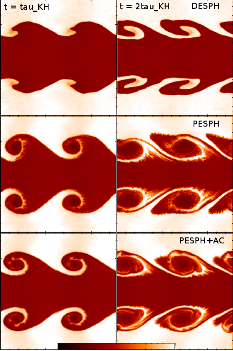
Figure 1: A density map of a Kelvin-Helmholtz test at time $t=\tau_{KH}$ (left) and $t=2\tau_{KH}$ (right). Top panels show the results from DESPH using a cubic spline kernel over $N_{ngb}=32$ neighbours, representing the hydro-solver used in our published cosmological runs. The middle panels show the new PESPH with an optimal $N_{ngb}=128$ quintic kernel, and the bottom panels use the time-dependent artificial viscosity following Cullen & Dehnen (2010) and artificial conduction, while the other runs use a constant parameter for the artificial viscosity. All runs start with an initial condition in which the relative velocity between two fluids is $160\ \mathrm{km/s}$ and the velocity perturbation is $8\ \mathrm{km/s}$.

The top and middle panels of Figure 1 compare the behaviour of DESPH and PESPH at $\tau_{KH}$ and $2\tau_{KH}$. The improvements of PESPH are significant. At the Kelvin-Helmholtz time-scale $\tau_{KH}$, the characteristic wave-like feature of KHI in the PESPH simulation have grown to a scale consistent with mesh based results (Read et al., 2010; Murante et al., 2011) and also the predictions of linear perturbation theory (Agertz et al., 2007). The PESPH simulation also shows efficient mixing of the fluid along with the growth of curled structures. In the DESPH run, however, the instability barely grows at $\tau_{KH}$, and the mixing is hardly seen even at later times (not plotted).

In the bottom panel of Figure 1 we rerun the PESPH simulation but switch the prescription of artificial viscosity to the time-dependent particle-by-particle treatment of Cullen & Dehnen (2010), and also apply artificial conduction. The new viscosity is known to significantly reduce unnecessary dissipation owing to velocity noise from turbulent regions and yet still maintain the ability of shock capturing. Since the physical conditions in KHI tests are mostly shock-free, the new viscosity only shows some minor effects at the contact surfaces at $2\tau_{KH}$. The differences, however, are much smaller than those between SPH formulations.

3.2 The blob test

Another classic numerical test involves putting a spherical gas cloud of uniform density into a fast moving hot medium, which is in pressure equilibrium with the cloud. It mimics the realistic situation of a shocked wind passing through cold dense gas, and it involves important physical processes such as ram-pressure stripping, fluid instabilities, and mixing. Again we take the initial condition from the Wengen test suite. The simulation is performed within a periodic tube with dimensions $x,y,z=2000,2000,6000$ kpc; the initial density of the cloud is 10 times that of the surrounding medium. The relative velocity of the two phases of gas is characterised by a Mach number of 2.7.

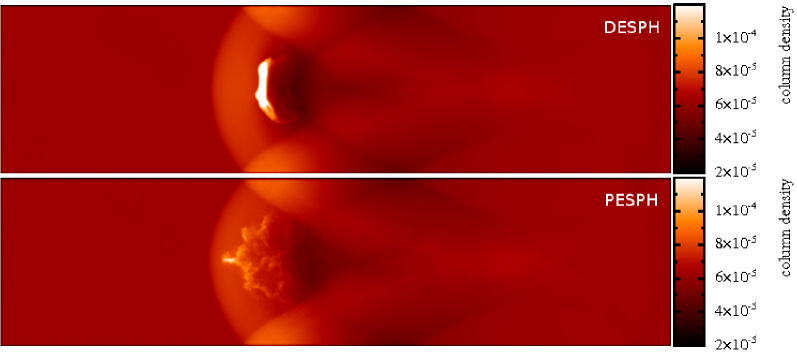
Figure 2: A density map of the blob tests at $\sim\tau_{KH}$ from the DESPH (upper) and PESPH (lower) methods.

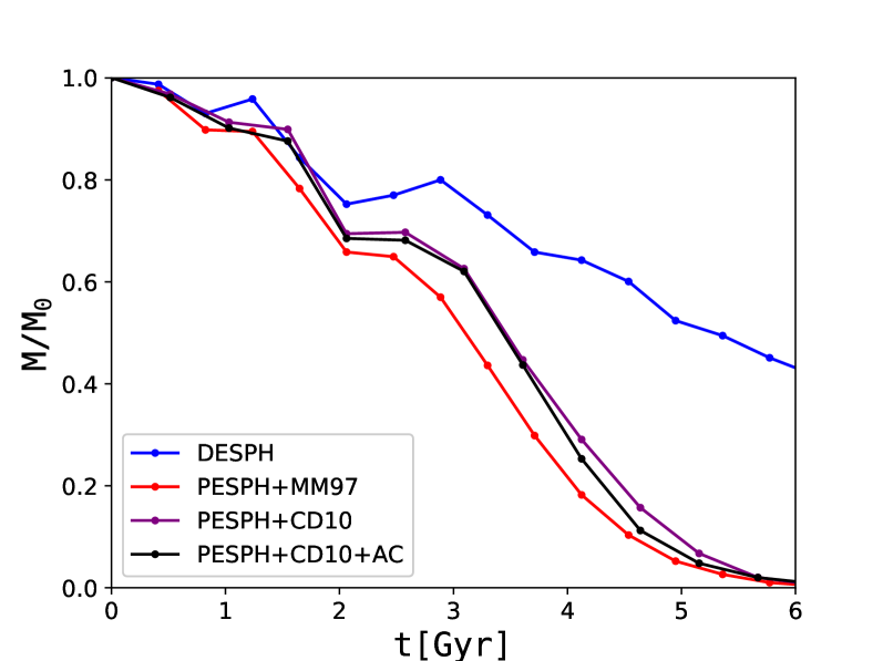
Figure 3: The evolution of cloud mass. The different lines correspond to simulations that use different numerical algorithms as labelled. See text for a full description of the different models. The cloud quickly loses mass in all the PESPH simulations owing to enhanced mixing between cold and hot gas.

Figure 2 shows the morphology of the gas cloud at around $\tau_{KH}$. Though the cloud in the DESPH run is deformed owing to the impact of the wind shock, the cloud particles still stick together, hardly mixing with the surrounding gas - a behaviour similar to that shown in the KH tests. In contrast, the clouds simulated using PESPH have clearly dissembled and dissipated into the hot medium. The predicted morphology agrees with mesh based results (e.g., Agertz et al., 2007).

Figure 3 shows the mass of the cloud as a function of time. Following Agertz et al. (2007), we define cloud as all those particles that have a density over 0.64 of its original density ($\rho>0.64\rho_{c}(t=0)$) and a temperature that is below 0.9 of the ambient temperature ($T<0.9T_{amb}$). The blue line uses the DESPH formulation with a constant viscosity and without artificial conduction. All the other lines use the PESPH formulation. The red line (PESPH-MM97) uses the Morris & Monaghan (1997) viscosity. Both the purple (PESPH-CD10) and the black line (PESPH-CD10-AC) use the Cullen & Dehnen (2010) viscosity, but the black line also uses artificial conduction. The evolution of the cloud mass is similar in all the PESPH simulations and is similar to our results. The clouds in these simulations lose mass quickly and are mostly destroyed after $6\ \mathrm{Gyrs}$, when we stop the simulations. The cloud in the DESPH simulation, however, loses mass at a slower rate and retains more than 40% of its mass at the end of the simulation.

In summary, with the new pressure-entropy formalism of the equations of motion, the performance of our SPH code in both the KHI tests and the blob test agrees with those from the mesh-based codes (e.g. Agertz et al., 2007; Sijacki et al., 2012), and agrees with the improvements seen in Hopkins (2013) and Hopkins (2015), who also showed it improved many other tests. These results demonstrate the successes of PESPH in effectively removing the artificial surface tension at fluid interfaces that leads to over suppression of fluid instabilities and mixing, which has been a long-standing problem with the DESPH formalism. Our results also show that our choices of artificial viscosity and artificial conduction only has a sub-dominant effect in these standard tests (see Appendix A for details).

4 COSMOLOGICAL SIMULATIONS

The standard tests above have shown that the new PESPH formalism leads to significant improvements in correctly resolving fluid mixing at contact discontinuities. Now we ask the question of whether these improvements would significantly change the results from realistic cosmological simulations. Most of the idealised tests are conducted at resolutions that are far higher than those typically obtained in galaxy formation simulations. At realistic resolutions the differences could be much less. Furthermore, the dynamical processes in cosmological simulations involve complicated interactions between multiphase baryons, e.g., cold gas accretion through cosmic filaments, hot halo gas formed by shock heating, cooling flows from the hot gas, and galactic winds. The hydrodynamical instabilities and gas mixing could change both the accretion rate and average cooling efficiency within the halo and possibly alter the entropy structure as well as the star formation history of the halo. For example, in previous SPH simulations, e.g., Kereš et al. (2009a), sub-resolution clumps of cold gas are shown to orbit within the hot haloes and rain down upon the central galaxy. This “cold drizzle”, which is thought to be a numerical artefact owing to the inefficiency of standard SPH in multi-phase mixing and stripping (Kereš et al., 2012; Nelson et al., 2013), could artificially enhance cool gas accretion and the star formation rate. Therefore, the poor numerical behaviour of the traditional SPH for these important processes adds uncertainties to the interpretation of the simulation results. However, given all the other important non-linear processes, such effects could be sub-dominant. Therefore, it is essential to examine how the changes introduced by PESPH may affect cosmological conclusions drawn from our previous simulations.

4.1 Numerical models

For cosmological simulations, the GADGET-3 code calculates the gravitational forces between all particles using a tree-particle-mesh algorithm, which allows the code to probe a large dynamic range efficiently. The dynamics of the gas particles is further determined by the SPH algorithm. Physical processes such as cooling and heating, star formation, feedback and metal enrichment play crucial roles in galaxy formation and evolution. However, to understand these processes, we must add sub-grid models on top of the hydrodynamical equations, because they occur on scales much below the spatial resolution of the simulation. Some of the sub-grid models have led to successes in matching observed data, and have become routinely incorporated in cosmological simulations. The specific models that we use have been described in detail in Oppenheimer & Davé (2006) and Oppenheimer & Davé (2008). Here we give a brief summary.

Apart from the dynamical heating processes owing to adiabatic compression and viscosity, an additional heat source implemented in our code is photoionisation whose rate depends on the UV background at different redshifts. To compute the radiative cooling, we tabulate the cooling rate as a function of discrete values of density and temperature, assuming ionisation equilibrium and primordial composition and interpolate. We allow the thermal energy of each particle to change with a cooling rate obtained from this look up table based on its thermodynamic properties. The look up table is updated to account for changes in the radiation background with redshift. When the particle is metal enriched, an additional metal cooling term is added to the total cooling rate.

In our previous work, the cooling rate is tabulated as a function of metallicity and density from the collisional ionisation equilibrium models of Sutherland & Dopita (1993) in the presence of the Haardt & Madau (2001) (HM01) ionising background. Wiersma et al. (2009) computed radiative cooling rates from 11 elements under the CMB and HM01 background. Subsequently, Haardt & Madau (2012) updated their estimate of the UV background by including several new components to their radiative transfer code CUBA. Motivated by these recent works, we have adopted the Wiersma et al. (2009) non-CIE cooling rates computed in the presence of the HM12 background. One of our main goals here is to investigate how this simulation, named as PESPH-HM12, differs from simulations that employ the hydrodynamics and cooling model that we used previously.

Our star formation model is adopted from Springel & Hernquist (2003). In this sub-grid model, a gas particle is treated as a two-phase particle, i.e., it becomes an ISM particle, when the overall density of the particle reaches a certain threshold. Based on the model of McKee & Ostriker (1977), we treat the gas particle as if it contains many cold clouds in pressure equilibrium with the surrounding warm ionised intermedium gas. The thermodynamic properties of the two phases are calculated separately following on analytical treatment of evaporation and condensation. These ISM particles are the sites where stars can form. The star formation rate is proportional to the square of the cold phase density and is calculated on a particle-by-particle basis, with the star formation time-scale fixed to match the observed Kennicutt law (Kennicutt, 1998). Collisionless particles representing groups of stars are allowed to form at each timestep, with a probability determined from the star formation rate. The star particle is either spawned from an ISM particle, taking away a fraction of its mass, or entirely converted from the gas particle, depending on how much mass is left in the ISM particle. The feedback from type II supernovae is added back to the hot phase assuming an instantaneous recycling approximation.

The metal enrichment model is an updated version of Oppenheimer & Davé (2008), in which three main sources of metals, type II SNe, type Ia SNe and AGB stars, are considered. The simulation now tracks the metallicity of four species C, O, Si, Fe separately, to account for the different enrichment effects of the alternative sources. At each timestep, each ISM particle is self-enriched by type II SNe, which occurs at a rate proportional to the star formation rate, assuming an IMF. For the Chabrier (2003) IMF we adopt in these simulations, we assume that stars with an initial mass larger than $10M_{\odot}$ end as a type II SNe, which gives a mass fraction of 0.18 immediately recycled upon star formation. The feedback from type Ia SNe and AGB stars returns metals and mass to the nearest gas particles on a delayed time-scale.

Previous simulations (Kereš et al., 2005, 2009b) have shown that simulations that implement the above ISM and star formation models produce a global SFR that is too high compared to observations. This motivates some form of feedback that suppresses either gas accretion or star formation. A full description of these models is beyond the scope of this paper but we will summarise the important points. We employ the hybrid energy/momentum-driven wind model (ezw model) (Davé et al., 2013), which is a slightly modified version of the momentum-conserving wind model (vzw model) used in our previous work (Oppenheimer & Davé, 2008; Davé et al., 2010, 2011a, 2011b), as our favoured wind model. The vzw model and ezw model have made predictions that match a range of observations, including IGM enrichment at high redshift observed through $C_{IV}$ systems (Oppenheimer & Davé, 2006, 2008), high redshift absorption systems (Oppenheimer & Davé, 2009), mass metallicity relations (Finlator & Davé, 2008), and the galactic stellar and HI mass functions at $z=0$ (Davé et al., 2013).

We assume in our fiducial outflow model that the outflow rate is related to the SFR by a mass loading factor $\eta$:

$$\dot{M}_{wind}=\eta\times SFR$$ (24)

The numerical implementation of outflows is analogous to that of star formation. Each ISM gas particle is a candidate for launching a wind, the probability of which is $\eta$ times the probability assigned for star formation, and is probabilistically determined for each particle at each timestep. Once it is launched, a velocity boost of $v_{w}$ is added to the particle in the direction of $\mathbf{v_{i}}\times\mathbf{a_{i}}$, where $\mathbf{v_{i}}$ and $\mathbf{a_{i}}$ are the velocity and acceleration of the particle before launch, as outflows are often seen perpendicular to the disc where interactions with the cold dense ISM are minimised. All hydrodynamical interactions relating to the particle are turned off for $1.95\times 10^{10}/v_{w}$ years or until the particle has reached a density that is below 10% of the critical density for star formation. Since the resolution in the ISM region is insufficient to correctly model hydrodynamical interactions (Dalla Vecchia & Schaye, 2008), this decoupling from hydrodynamical forces allows galactic winds to develop and avoids calculating numerically inaccurate interactions.

The free parameters $\eta$ and $v_{w}$ are crucial to the wind models. The scaling for momentum conserving winds are motivated from Murray et al. (2005), which suggested a wind speed that scaled with the galaxy velocity dispersion:

$$\eta=\left\{\begin{array}[]{ll}\frac{\sigma_{0}}{\sigma}\frac{75\ \mathrm{km/s}}{\sigma}(\sigma\leqslant 75\ \mathrm{km/s})\\ \frac{\sigma_{0}}{\sigma}(\sigma\geqslant 75\ \mathrm{km/s})\end{array}\right.$$

$$v_{w}=4.29\sigma\sqrt{f_{L}-1}+2.9\sigma$$ (25)

where $f_{L}$, depending on the metallicity, is the luminosity factor in units of the galactic Eddington luminosity, constrained by observations (Rupke et al., 2005), and $\sigma_{0}=150$km/s is a normalisation factor that is adjusted to match high-redshift IGM enrichment (Oppenheimer & Davé, 2008).

The lower limit $\sigma_{vzw}=75$km/s in the above equation distinguishes between momentum-driven scalings and energy-driven scalings. The momentum-driven mass-loading factor, which scales with $\sigma^{-1}$, applies to relatively large systems where outflows are driven primarily by the momentum flux from young stars and supernovae while the thermal energy from supernova is dissipated too quickly to become dynamically important. However, in dwarf galaxies with a $\sigma$ below this limit, we assume that energy feedback from supernovae starts to dominate, based on analytical and numerical models by Murray et al. (2010) and Hopkins et al. (2012). In this energy conserving regime, we assume $\eta\propto\sigma^{-2}$. As Davé et al. (2013) show, this hybrid scaling leads to better agreement with the low mass stellar mass function.

The velocity dispersion $\sigma$ is determined on-the-fly. We identify galaxies using a friends-of-friends algorithm that binds particles to their closest neighbours if they are within a linking length of 0.04 times the typical separation between dark matter particles. This linking length applies to all classes of particles, including dark matter, so it incorporates the inner regions of the dark matter halo. The velocity dispersion is evaluated from the total mass of the galaxy $M_{gal}$:

$$\sigma=200\left(\frac{M_{gal}}{5\times 10^{12}M_{\odot}}\frac{H(z)}{H_{0}}\right)^{1/3}\mathrm{kms^{-1}}$$ (26)

The velocity dispersion could also be computed for each galaxy explicitly, but uncertainties arise owing to poor resolution particularly in the inner regions of each galaxy. Moreover, numerical noise would in some cases yield a rather spurious $\sigma$ that would lead to unphysical results and when calculating $\sigma$ for satellite galaxies directly it is almost impossible to remove background material that belongs to the larger central galaxy. Therefore, we use the above empirical relation given that any errors that arise from using this relation are sub-dominant to the uncertainties that come from our assumptions of the wind model itself.

The FoF algorithm is slightly different from what we used before. Since $\sigma$ and thus the mass of groups is crucial to our feedback model, we empirically adjust the linking length in the FoF algorithm so that the mass of groups found using our old and new algorithms are on average the same, so that the scaling relations that we adopt for our wind prescription still hold.

4.2 Simulation setup

To separate the effects of changing numerical and physical details, we have run two classes of simulations: nw simulations that have no stellar feedback, i.e. no galactic winds; and ezw simulations that employ our fiducial momentum-driven wind model. Each of the two classes contain simulations that use different numerical algorithms. We have run two nw simulations in which no feedback is added: one (DESPH-nw) with the original numerical algorithms and the other one (PESPH-nw), which uses all the improved schemes. For the ezw model, we have run the following simulations: 1. The DESPH simulation, representative of the simulations we have used in previous papers, uses the traditional density-entropy formulation from Springel & Hernquist (2003), a cubic spline kernel with $N_{ngb}=32$, and an artificial viscosity scheme with a constant $\alpha=1.0$ and the Balsara switch. 2. The PESPH simulation uses the pressure-entropy formulation derived by Hopkins (2013), a quintic kernel of $N_{ngb}=128$ and the M&M viscosity. The PESPH simulation also employs the timestep limiter from Durier & Dalla Vecchia (2012). In the PESPH simulation, we use the entropy weighted density only to evolve the hydrodynamics. For other density dependent physical processes such as cooling and star formation, we still use the unweighted density obtained from kernel smoothing (see below). 3. The PESPH-HM12 simulation is based on the numerical algorithms of the PESPH simulation, but it applies non-CIE metal cooling models combined with the HM12 ionisation background, instead of the CIE cooling model and HM01 background used in the other simulations. We also perform another simulation identical to PESPH-HM12 except using the old artificial viscosity to discuss its effects separately. 4. Our fiducial simulation, PESPH-HM12-AC, combines all the improvements from the other simulations and also employs the Cullen & Dehnen (2010) viscosity and artificial conduction. See Table 1 for a summary.

Table 1: Simulations and their adopted numerical and physical models

Simulation	Formulation	Kernel	Viscosity	Limiter	W09	UVBKG	AC	Feedback
DESPH-nw	DESPH	CS-32	$\alpha=1.0$	No	No	HM01	No	nw
PESPH-nw	PESPH	QS-128	CD10	Yes	Yes	HM12	Yes	nw
DESPH	DESPH	CS-32	$\alpha=1.0$	No	No	HM01	No	ezw
PESPH	PESPH	QS-128	M&M97	Yes	No	HM01	No	ezw
PESPH-HM12	PESPH	QS-128	M&M97	Yes	Yes	HM12	No	ezw
PESPH-HM12-AC	PESPH	QS-128	CD10	Yes	Yes	HM12	Yes	ezw

Our primary goal in this paper is to study how the new physical prescriptions in cooling and the improved numerical schemes affect our predictions from the same initial conditions. Therefore we focus on comparing the fiducial simulation PESPH-HM12-AC and our original version of GADGET3 - DESPH. The results from the other simulations provide information on how specific changes to the code affect certain changes in the simulated universe. For example, as shown later, PESPH when compared to DESPH demonstrates the efficiency of the new SPH formulation and a time-dependent viscosity in removing the pseudo dense gas clumps within galactic haloes; the PESPH-HM12 shows the effects of the new cooling model and the background.

In any cosmological simulation that uses the PESPH formulation, there are two ways of defining the density of an SPH particle (see section 2.1). It could be evaluated either by kernel weighted average as in traditional DESPH, or by entropy weighted average as in PESPH. Here we always use the traditional volume-derived density for any of the sub-grid models such as cooling and star formation, and also for all the post analysis on the simulation data. This is to avoid any bias towards high entropy particles that could lead to multi-valued densities in neighbouring particles. The entropy weighted density is only applied while solving the hydrodynamics. Oppenheimer et al. (2018) points out that this density choice could lead to considerable differences in some predictions (see their appendix D).

We assume a $\Lambda$CDM cosmology with parameters $\Omega_{m}=0.30,\Omega_{\Lambda}=0.70,h=0.7,\Omega_{b}=0.045,n=0.96,\sigma_{8}=0.8$ for all our simulations, as a compromise between WMAP7 (Hinshaw et al., 2009) and the Planck (Planck Collaboration et al., 2014) results. We performed simulations in a random periodic box of $50h^{-1}$Mpc on each side that contains $288^{3}$ gas and $288^{3}$ dark particles initially. The initial mass of each gas particle and dark particle are therefore $m_{gas}=9.3\times 10^{7}M_{\odot}$ and $m_{dark}=5.3\times 10^{8}M_{\odot}$. All simulations start at $z\sim 100$ and evolve down to $z=0$.

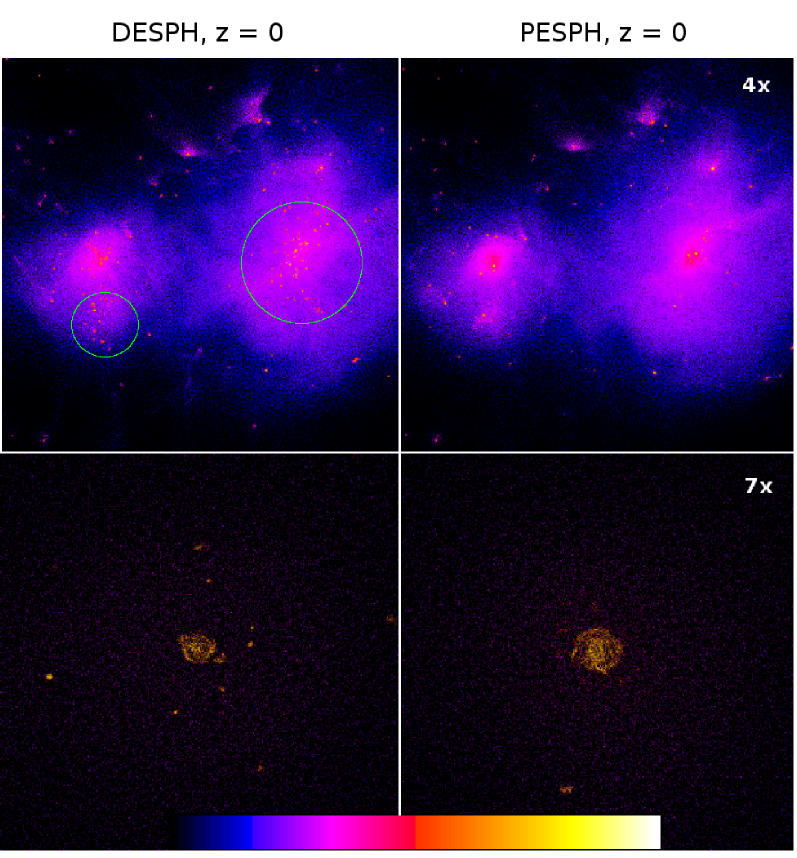
Figure 4: Two projected regions are extracted at $z=0$ from the DESPH (left panels) and PESPH (right panels) cosmological simulations to illustrate the impact of the new PESPH algorithm. Each panel shows a density map with a large dynamic range ($\rho/<\rho>=1{\rm\ to\ }10^{10}$). The simulations are performed within a periodic box with $50\ h^{-1}$ Mpc on each side. The labels ”4x” and ”7x” in the upper right corners of each panel indicate the power of magnification over the original box, corresponding to a size of $\sim 3.1h^{-1}$ Mpc and $\sim 0.4h^{-1}$ Mpc on both axes, respectively. Green circles highlight the differences between the snapshots compared.

Figure 4 compares the morphologies of simulated systems in two regions at $z=0$. The DESPH simulation has many distinct dense gas clumps orbiting within the diffuse hot gas halo. These sub-resolution clumps are especially prevalent in the massive haloes as shown in the upper left panel, where we plot the most massive halo from the simulation. This feature has also been noticed in the non-feedback simulations of Kereš et al. (2009a, b), who attribute this “cold drizzle” to numerical artefacts that would enhance cold mode accretion within massive haloes. In the PESPH simulation, these clumps break up and mix into the ambient gas more easily owing to enhanced fluid instabilities and more efficient mixing between fluid interfaces, and are thus effectively removed. Therefore, the PESPH formulation alone is sufficient for removing the cold blobs present in the traditional DESPH simulations, consistent with the findings of Hu et al. (2014). We also note that, in the bottom panels, PESPH produces a more extended gas disc in the centre. Vogelsberger et al. (2012) and Torrey et al. (2012) also found that galaxies in their moving mesh code AREPO are generally more extended and disc-like than those in DESPH simulations. However, whether there is a general trend on the size and morphology of individual galaxies in the PESPH simulation is beyond the scope of this paper owing to the limited spatial resolution of the simulations presented here.

5 Cosmic Baryons

5.1 The stellar mass - halo mass relation

Cosmological simulations without any feedback processes have been known to over-produce the stellar content of the universe (Davé et al., 2001; Springel & Hernquist, 2003). Simulations that only consider kinetic feedback from young stars and supernovae are able to reproduce the z=0 galactic stellar mass function (GSMF) below $M_{*}<10^{10.5}M_{\odot}$, yet still produce too many massive galaxies (Oppenheimer et al., 2010). The cold drizzle, i.e., dense sub-resolution clumps that do not mix efficiently with hot surroundings owing to numerical effects, could be accreted by the central galaxies on a short time-scale and enhance their star formation rate. In this section we examine to what extent the new numerical schemes affect the stellar content of the universe, and also the properties of the simulated galaxies.

To study the statistics of simulated galaxies and haloes, we use SKID (Spline Kernel Interpolative Denmax) to identify bound groups of star and ISM particles (Kereš et al., 2005; Oppenheimer et al., 2010) as simulated galaxies. We will focus on those SKID groups that are above the mass limit of $M_{*}>6.0\times 10^{9}M_{\odot}$, equivalent to a total mass of 64 original gas particles. This choice is motivated from extensive convergence tests (Finlator et al., 2006). Furthermore, we identify haloes using a spherical overdensity (SO) algorithm (Kitayama & Suto, 1996; Kereš et al., 2005). In SO, we start from the most bound particle within each SKID galaxy and search for all particles within a spherical density contour within which the mean interior density equals the virial density. Then we join haloes to their larger companions if the centre of the smaller halo falls within the virial radius of its larger companion. In our simulations, we typically identify $\sim 10^{3}$ galaxies at $z=4$ and $\sim 10^{4}$ galaxies at $z=0$.

For each halo found by SO, we derive its virial mass as well as the mass of its central galaxy. The stellar mass and the halo mass follows a very tight trend (Yang et al., 2012; Moster et al., 2013) that indicates how efficiently stars form in haloes of different masses at different times. In Figure 5 we examine how this stellar mass - halo mass relation (SMHM) is affected by the different numerical schemes.

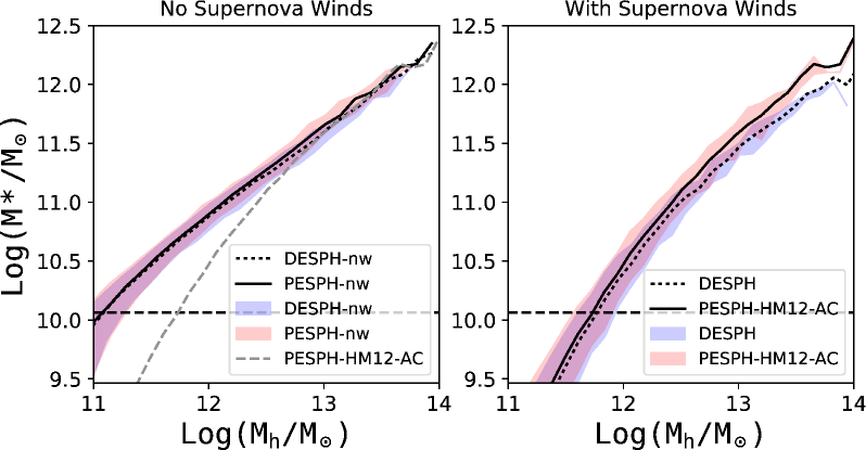
Figure 5: The stellar mass - halo mass relations from simulations without supernova feedback (left panel) and with supernova feedback (right panel). In each panel, the dotted line and the blue shaded region are from DESPH simulations, and the solid line and the red shaded region are from PESPH simulations. The shaded region encloses 95% of all galaxies in the corresponding mass bin. In the left panel, we reproduce the relation from our fiducial simulation as a grey dashed line for comparison. The black dashed horizontal line in each panel indicates the stellar mass resolution limit for galaxies.

The SMHMs from simulations that do not have any feedback (DESPH-nw and PESPH-nw) are distinct from those that employ the ezw momentum-driven wind model. The galaxies in the nw simulations are much more massive in nearly all the haloes and especially so in less massive ones. Between these two nw simulations, however, the differences are quite small, with PESPH-nw producing only slightly more stars in the most massive haloes. Compared to the nw simulations, the ezw wind model more efficiently suppresses star formation in lower mass haloes but has hardly any effect on the most massive ones. This trend with halo mass can be explained by differential recycling (Oppenheimer et al., 2010), i.e., the recycling time-scales for ejected wind particles in low mass haloes are much longer than those in massive haloes, where the wind particles quickly fall back to the centre of the potential, resembling a galactic fountain. Like in the nw simulations, the SMHMs in the ezw simulations are very similar, though the differences are more prominent. The median from PESPH-HM12-AC is less than 0.1 dex higher than DESPH across most of the resolved mass range. Only in the most massive haloes are the differences larger, where the galaxies in the PESPH-HM12-AC simulation are around 30% more massive than their counterparts with DESPH. In the latter sections we will show that this owes to an enhanced baryonic accretion rate in the PESPH simulations.

5.2 Hot gas fractions

The new hydrodynamic schemes have the potential to alter the properties of the hot gas within galaxy groups, as the PESPH formulation could enhance the mixing of cold gas into hot corona gas and the new viscosity scheme captures shocks more accurately. Since the X-ray emitting gas in groups is mostly heated by shocks, its properties could be sensitive to the numerics.

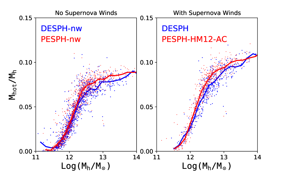
Figure 6: The mass fractions of hot gas ($T>5\times 10^{5}K$) in simulated haloes as a function of their halo mass. Haloes from the DESPH simulations are plotted in blue and those from the fiducial PESPH simulations are plotted in red. The solid lines show the running medians. In the left panel we compare the two nw simulations and in the right panel we compare the two ezw simulations.

In Figure 6 we compare the mass fraction of hot gas ($T>5\times 10^{5}K$) in individual haloes. In general, the hot gas fraction increases with the halo mass because of the deeper potential and higher virial temperature. The relations in both nw simulations agree surprisingly well. The agreement between the two ezw simulations is also good, though the slope is slightly steeper in the PESPH simulation. Also, compared to the nw runs, the stellar feedback in the ezw runs only contributes a little extra hot gas to massive groups, as also found in Ford et al. (2014) and Liang et al. (2016), owing both to the small mass loading factors in massive galaxies and the short wind recycling time-scales. The differences between the ezw simulations seems to maximise around $M_{h}\sim 10^{13}M_{\odot}$, which is the key regime for galaxy transformation. However, these differences are small.

5.3 Baryonic accretion

The star formation history of the universe is closely linked to how galaxies acquire their gas. The particle nature of SPH facilitates the straightforward study of the accretion histories of galaxies. By tracking individual particles through simulation outputs we are able to study the thermal histories of accreted material that assemble into the simulated galaxies. We define an accretion event to occur when a gas particle resides inside a resolved SKID group ($M_{gal}>64m_{gas}$) when that SKID group did not contain the gas particle in the previous output. For each simulation we have 75 outputs from $z=4$ to $z=0$. We subdivide the accretion into three major channels (Kereš et al., 2005, 2009a; Oppenheimer et al., 2010; Roberts, prep). When a gas particle is found in a resolved galaxy for the first time, we subdivide the accretion as either hot pristine gas accretion (hot mode), if the maximum temperature $T_{max}$ of the particle reached at least $2.5\times 10^{5}$ K at any time before accretion, or cold pristine gas accretion (cold mode) if not. Once a particle accretes we reset its $T_{max}$ to zero and only allow $T_{max}$ to change if the particle leaves the star-forming region. If an accreted particle has been launched as a wind particle previously, we define the accretion event as wind re-accretion (wind mode). Note that the accretion tracking program used here (Roberts, prep) also classifies accretion into a few other sub-dominant channels (less than 10%), but we omit them from the plot for the purposes of this paper and do not consider them further.

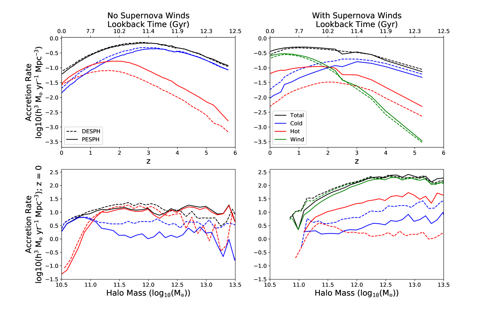
Figure 7: Upper panels: Global accretion rate as a function of redshift from $z=6$ to $z=0$ in our simulations. We compare the two nw simulations in the left panels and the two ezw simulations in the right panels. The DESPH simulations and the PESPH simulations are plotted as dotted lines and solid lines, respectively. We divide the accretion into three channels defined in the text, namely, cold mode pristine accretion (blue), hot mode pristine accretion (red) and (in ezw simulations where galactic winds are added using a sub-grid prescription) wind re-accretion (green). The black lines in each panel indicate the total accretion rates. Lower panels: Global accretion rate as a function of the host halo mass at $z=0$.

The top panels in Figure 7 show how galaxies acquire their gas through the three major accretion channels: cold (blue), hot (red) and wind re-accretion (green) across cosmic time for PESPH and DESPH with (ezw) or without (nw) supernova winds. The most significant change from our original DESPH formulation is that the new PESPH formulation boosts the hot accretion rate by a large fraction at nearly every redshift for both the nw and ezw models. In the nw simulations, galaxies accrete their gas through either cold accretion or hot accretion. Since there are no winds, only a small amount occurs owing to reaccretion of tidally stripped gas, which we do not plot. In the PESPH simulation, cold accretion is suppressed after $z=3$ by a small fraction, but hot accretion is consistently enhanced by half a dex. The total accretion rates, however, are very similar between the two simulations.

Figure 7 (bottom panels) show how these process depend on halo mass at $z=0$. The accretion rate is measured by counting the amount of accretion onto each halo during a small time window. Differences in the cold/hot accretion rates are obvious only in haloes with $\log(M_{h}/M_{\odot})>11.0$, and the enhancement in hot mode accretion increases with halo mass. In smaller mass haloes, galaxies acquire their baryons mostly from cold streams that are never shocked above the temperature threshold of $2.5\times 10^{5}$ K. The accretion rates in these haloes are hardly affected by the SPH formulation. These haloes are generally devoid of a hot corona, so that the hydrodynamical interactions between cold and hot gas are unimportant. In the ezw simulations, wind-reaccretion starts to dominate after $z=2$. Although the hot accretion rate is strongly enhanced at $\log(M_{h}/M_{\odot})>10.5$, the impact of the new numerics on the dominant wind-reaccretion rate is insignificant, and the impact on cold accretion rates is small.

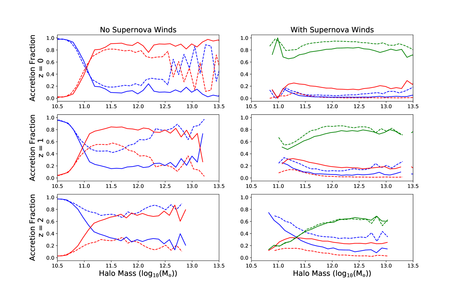
Figure 8: In these plots we compare the fractional accretion rate as a function of halo mass at $z=0,1,2$ (upper, middle and lower panels). As in fig. 7, the left panels compare the two nw simulations and the right panels compare the ezw simulations. The dotted and solid lines in each panel correspond to the DESPH and PESPH simulations, respectively.

Figure 8 shows how the instantaneous fractional accretion rate through the three channels depends on halo mass at different redshifts. There is a fractional enhancement of hot mode accretion in both the nw and ezw simulations at all redshifts when using the PESPH formulation. This numerical effect is most prominent in the nw simulations at $z=1$ and $z=2$: In the original DESPH simulation, cold mode accretion dominates over hot mode accretion in nearly all haloes; however in the PESPH simulation, hot mode accretion starts to dominate in haloes with $\log(M_{h}/M_{\odot})>11$. In the ezw simulations, wind-reaccretion still dominates at $z=0$ and $z=1$ and is not much affected by the SPH algorithm. As in the nw simulations, PESPH significantly enhances hot mode accretion, making it comparable to cold mode accretion in intermediate to massive haloes. The results for DESPH are similar to those of Kereš et al. (2009a, fig. 8) as expected, while those for PESPH are closer to the earlier results of Kereš et al. (2005, fig. 6), though with a cold-to-hot transition shifted downward by $\sim 0.3$ dex in halo mass.

In previous cosmological simulations that use the traditional DESPH formulation (Kereš et al., 2009a), the cold dense gas clumps that form either by spuriously numerically enhanced thermal instabilities or stripping contribute a considerable amount of pseudo cold accretion as they fall onto the central galaxy. The PESPH formulation allows efficient mixing between these cold structures and their hot surroundings, prevents these cold clumps from falling onto the galaxies, thereby suppressing cold accretion. Besides, the enhanced mixing lowers the thermal energy of the hot halo gas, which can, therefore, cool more efficiently, allowing for more hot mode accretion. This provides a possible explanation for the differences between the accretion rates in the DESPH and PESPH simulations. The new artificial viscosity reduces artificial heating from numerical noise in the velocity field where the flow is non-convergent, but increases heating by capturing shocks more accurately. However, it is challenging to measure its net effects quantitatively. The increase in hot gas fractions for PESPH shown in Figure 6 probably indicates that some of the increase in hot mode accretion, which comes at the expense of a decrease in cold mode accretion (Figure 7), owes to more shock heated gas.

The PESPH simulations retain the key qualitative findings of our earlier papers Kereš et al. (2005, 2009a); Oppenheimer et al. (2010): in nw simulations, cold mode accretion dominates galaxy growth at low halo masses and high redshifts; in ezw simulations, wind recycling dominates galaxy growth in massive haloes at low redshifts. However, hot mode accretion rates are sensitive to the difference between DESPH and PESPH, and these differences can shift the redshifts or masses at which hot accretion comes to dominate over cold accretion. This result is consistent with findings from AREPO simulations Nelson et al. (2013).

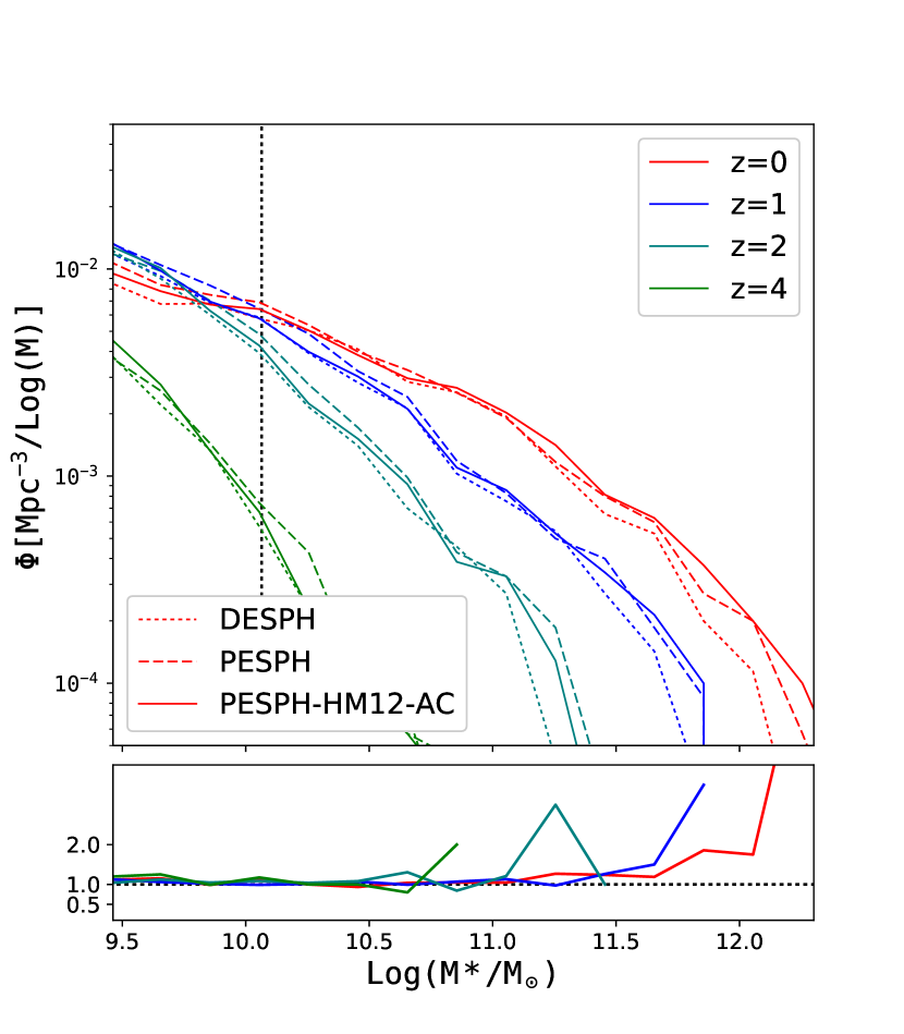
Figure 9: The upper panel shows the galactic stellar mass functions (GSMFs) at $z=0$(red), $z=1$(blue), $z=2$(teal), and $z=4$(green). The dotted, dashed, and solid lines correspond to the DESPH, PESPH, and PESPH-HM12-AC simulations. The dotted vertical line shows half of the resolution limit (32 gas particles) for SKID galaxies. The bottom panel shows the ratio of the number densities of galaxies from the PESPH-HM12-AC simulation to the DESPH one at each stellar mass bin. The same colour scheme is used as in the upper panel.

5.4 Galaxies

In Figure 9 we show the galactic stellar mass functions (GSMFs) at four redshifts. Despite the differences in the numerical schemes and the cooling model, the GSMFs in low mass galaxies with $M_{*}<10^{10.5}M_{\odot}$ are nearly identical for all three simulations compared here at any redshift. In the most massive galaxies, the numerical scheme does make a small yet noticeable difference. Both PESPH and PESPH-HM12-AC use the pressure-entropy formulation and produce slightly more massive galaxies than DESPH, but the differences between these two simulations are quite small. Even though the growth of massive galaxies is most likely dominated by physical assumptions rather than the numerics, this change at the high mass end could provide further constraints on a proper quenching model to suppress star formation in these massive haloes. As Figure 5 shows, the star formation in low mass galaxies is strongly regulated by our kinetic feedback scheme. The results of Oppenheimer et al. (2010) show that a slight change in the feedback model leads to very different stellar mass functions. Here our results confirm that feedback is crucial to explaining the observed stellar mass function regardless of the numerical errors introduced by the traditional SPH formulations.

The results on the GSMFs are consistent with our previous results on the accretion rates and the stellar mass - halo mass relation. The stellar mass growth depends on the total accretion onto the galaxies. Even though the hot mode accretion is considerably enhanced by the new SPH techniques (Figure 7), it is compensated by the reduced cold accretion. The total accretion rate, which is dominated by cold mode accretion at high redshifts and by wind re-accretion at low redshifts, hardly changes.

By comparing the traditional SPH and ANARCHY SPH, Schaller et al. (2015) also find that the GSMFs are very insensitive to PESPH and other numerical improvements. However, they find that ANARCHY SPH produces slightly less massive galaxies at z = 0, opposite to our findings. Though the ANARCHY scheme is very similar to our fiducial SPH scheme, they use a feedback prescription that is very different from us. It is not straightforward to determine how different feedback schemes are specifically affected by even the same numerical changes.

Besides the stellar mass functions, we have examined the global star formation histories in our simulations, as well as the properties of individual galaxies, such as the relation between the specific star formation rate (sSFR) and stellar mass, the gas phase mass-metallicities relation, and the gas fraction as a function of galactic mass. None of these results are strongly affected by either the numerics or the non-equilibrium cooling model/HM12 background. Detailed comparisons can be found in Appendix C and Appendix D.

6 Intergalactic and Circumgalactic Medium

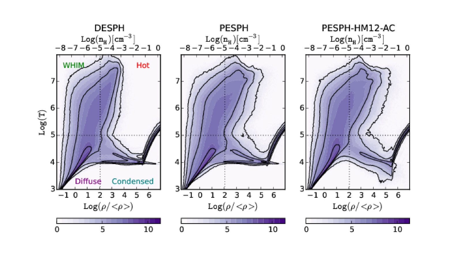
Figure 10: Density-temperature phase diagrams from the DESPH, PESPH and PESPH-HM12-AC simulations at $z=0.25$. The grey scale indicates the gas particle number density. The dotted lines overplotted in each panel divide the baryons into different phases following Davé et al. (2010). The upturn starting from $n_{H}>0.13\ \mathrm{cm^{-3}}$ results from our assumption of an effective equation of state for multi-phase interstellar medium gas (Springel & Hernquist, 2003). Despite noticeable differences in a few regions, the distribution of gas particles in the three simulations are quite similar, indicating that the global gas properties are insensitive both to changes in the SPH algorithm and the cooling physics.

In this section we restrict our discussion to the simulations with galactic winds (ezw). Relative to our older DESPH prescriptions, we examine the impact of the pressure-entropy formulation, the Wiersma et al. (2009) metal cooling and the HM12 UV background (PESPH-HM12), and the changes to the artificial viscosity and the artificial conduction (PESPH-HM12-AC).

The thermodynamic properties of baryons in the simulated volume can be conveniently studied by looking at the phase diagram (Figure 10), in which the SPH particles are binned in density - temperature space. Following Davé et al. (2010), we divide all gas particles into five categories depending on their locations in the phase diagram. To separate regions in the diagram, we choose a constant temperature threshold of $T_{th}=10^{5}$ K and a redshift dependent overdensity threshold of $\delta_{\rho}$ defined by (Kitayama & Suto, 1996):

$$\delta_{\rho}=6\pi^{2}(1-0.4093(1/f_{\Omega}-1)^{0.9052})-1$$ (27)

where

$$f_{\Omega}=\frac{\Omega_{m}(1+z)^{3}}{\Omega_{m}(1+z)^{3}+(1-\Omega_{m}-\Omega_{\Lambda})(1+z)^{2}+\Omega_{\Lambda}}$$ (28)

The threshold reflects the overdensity at the boundary of a virialised halo and roughly separates gas within dark matter haloes from that outside them. The thresholds are shown as dotted lines in Figure 10. Though the classification is a simple one, tests have shown that the gas particles that fall in each region represent different baryonic environments (Davé et al., 2010). The lower left of the diagram consists mainly of diffuse primordial gas. Most of these gas particles lie on a well defined curve in the phase diagram, which is established by a balance between adiabatic cooling and photoionisation heating. A fraction of gas particles are shock heated when they collapse into the gravitational potential of dark matter sheets and filaments and are driven into warm-and-hot ionised gas outside of haloes (upper left) or fall into dark matter haloes and become hot halo gas (upper right). Radiative cooling later plays a critical role in the further condensation of gas into the condensed region (lower right) where SF can occur. In addition, some gas goes straight from the diffuse to the condensed region, i.e. cold mode accretion (Kereš et al., 2005, 2009a). The upturn in the densest region owes to multi-phase ISM particles with densities above the star formation density threshold of $n_{H}=0.13\ \mathrm{cm^{-3}}$, which follow an effective equation of state. All ISM particles are counted as condensed gas even if their temperatures pass $T_{th}$. The fifth baryonic phase is stars.

The global distributions are quite similar in all three simulations, indicating that the phase structure of baryons on a global scale is not significantly affected by the hydrodynamical formalisms or the radiative cooling model. In the hot dense region that represents shocked halo gas, simulations with the PESPH formulation extends the hot gas to higher densities, lowering their entropy. Since this hot gas is most responsible for X-ray emissivity, the enhanced density could lead to a considerable boost in X-ray luminosities in PESPH haloes at given mass (see section 6.4). The region near the point where gas phases intersect is also slightly affected. The phase diagrams of the PESPH and the fiducial PESPH-HM12-AC simulations resemble each other except in the condensed gas region. In the left and middle panel, the locus of particles at $T\sim 10^{4}$ K consists mostly of enriched gas particles for which the CIE metal line cooling becomes negligible at that temperature. In the PESPH-HM12-AC simulation, on the other hand, photoionised electrons from heavy elements allow these particles to cool further, until it establishes a density dependent thermal equilibrium. However, photoionisation suppresses metal line cooling in the warm, less dense gas, leading to noticeable differences at $n_{H}=10^{-5}$ to $10^{-4}\ \mathrm{cm^{-3}}$ and $T=10^{4}$ to $10^{5}\ K$.

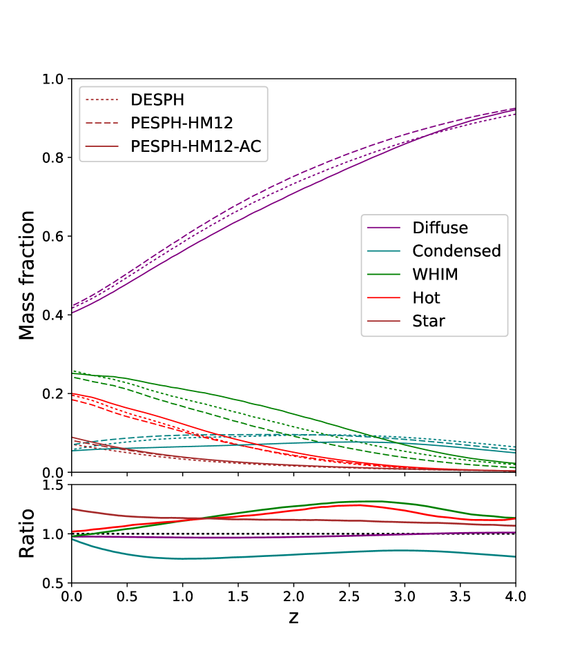
Figure 11: The upper panel shows the evolution of the different baryonic phases. We plot the mass fractions in each phase as a function of redshift for DESPH, PESPH and PESPH-HM12-AC simulations as dotted, dashed and solid lines, respectively. The purple, green, red, teal and brown lines represent cold diffuse IGM gas, warm and hot ionised medium, hot ionised halo gas, dense cold gas in galaxies and gas locked into stars, respectively. The definition of each phase is given in §6. The amount of gas in each phase in the different simulations is very similar at all times. The bottom panel shows the ratio of the mass fraction of each phase in the PESPH-HM12-AC simulation to the DESPH one, as a function of redshift. The same colour scheme is used as in the upper panel.

For a more quantitative comparison, Figure 11 shows how the fraction of baryons in each phase changes over cosmic time. The mass fractions of the four gas phases plus the stellar component from the three simulations are shown as a function of redshift. Baryons start in the diffuse phase and enter the other phases as structure grows (Davé et al., 2010). A striking agreement is seen between these different simulations. The total amount of hot gas in PESPH is only slightly larger than in the DESPH, despite the fact that there is a noticeable increase in the hot gas at higher densities in the PESPH simulation (Figure 10). The fiducial PESPH-HM12-AC simulation is the most different from the other simulations. The diffuse gas fraction is lower since $z\sim 2.5$ when the WHIM and hot fraction has increased by nearly 30% and declines thereafter. The WHIM and hot phase in our simulations are formed primarily from shock heated gas, but also has contributions from galactic winds. These changes are most likely caused by the Cullen & Dehnen (2010) viscosity, which reacts faster to converging flows than the M&M97 viscosity. It makes the new viscosity more sensitive to accretion shocks around the filaments and the wind particles as soon as they recouple hydrodynamically. Indeed, when we track the dynamical histories of individual particles in some smaller test simulations we find that the wind particles slow down more quickly with the new viscosity.

Observationally the intergalactic medium is often probed using quasar absorption line spectra. To mimic this technique, we take sightlines through our simulation box and generate absorption spectra using SPECEXBIN. A thorough description of this method can be found in Oppenheimer & Davé (2006), we only give a brief summary here. We take lines of sight through the periodic box, and divide them into tiny redshift bins, so that each “pixel” of the spectra corresponds to one redshift bin. In each bin, the optical depths of various species are computed based on the smoothed local physical properties such as density, temperature, metallicity and background radiation. These properties are evaluated by smoothing over all nearby SPH particles within the smoothing kernel. We adjust the HI optical depth later by matching the evolution of Lyman $\alpha$ flux decrements to observations following Davé et al. (2010). We multiply all the optical depths by a redshift independent correction factor of 0.62 to DESPH and PESPH results and a factor of 0.31 to PESPH-HM12 and PESPH-HM12-AC results. This is equivalent to enhancing the background ionising flux. The value chosen for the simulations using the HM01 background is close to that used in Davé et al. (2010), which also assumes the HM01 background. However, when we use the HM12 background, a larger correction is needed to match the flux decrement constraints, indicating that ionising photons from the HM12 background are insufficient to ionise the Lyman $\alpha$ forest at low redshift. This is consistent with the findings of Kollmeier et al. (2014).

To understand the absorption on different scales, we generate two kinds of absorption spectra. First, we take 70 random lines of sight, each of which wraps around the simulation box a few times until it covers a redshift range from $z=0$ to $z=2$. These spectra are used to normalise the radiation background, study the evolution of elements, and study the global column density distributions of several species. We normalise the background UV field intensity to match the observed mean Ly$\alpha$ opacity. Second, we take short targeted lines of sight surrounding haloes, following Ford et al. (2013). We select 250 haloes that fall in the mass range $11.75<\log(M_{h}/M_{\odot})<12.25$ out of each simulation at $z=0.25$. For each halo, we take short sightlines that penetrate the halo at different radii. We generate four spectra for each of the 12 impact parameters ranging from 10 kpc to 300 kpc. This procedure results in 12,000 short spectra for each simulation. We apply COS instrumental S/N and resolution to all spectra, long or short, so that our statistics are comparable to those obtained from real COS spectra and also directly comparable to Ford et al. (2013).

We fit Voigt profiles to each spectrum using AUTOVP (Davé et al., 1997). Each ion is fit separately. AUTOVP then outputs the column density and equivalent width (EW) for each fitted feature. We combine individual metal lines into systems if their line centres are closer than 100 km/s in velocity space, by adding the column densities and EWs to the largest feature. For short sightlines surrounding the haloes, we focus our study on features within $\Delta v\pm 300km/s$ of the central galaxy. This range covers the vast majority of absorption within the halo (Ford et al., 2013).

6.1 The Lyman-alpha forest

The Ly$\alpha$ forest is a distinct feature in high redshift quasar spectra that arises from absorbers that lie along the line of sight to distant quasars. The Ly$\alpha$ forest has been an important observational constraint on the $\Lambda$CDM cosmology and provides valuable insights on structures in the intergalactic and circumgalactic medium (Kollmeier et al., 2003; Davé et al., 2010; Peeples et al., 2010a, b; Kollmeier et al., 2014). Davé et al. (2010) show that the statistics of Ly$\alpha$ absorbers is insensitive to the feedback prescription, despite the strong dependence of the global star formation history and the halo enrichment on feedback. In this section we study the robustness of the predicted Ly$\alpha$ column density distribution to different numerical and physical schemes.

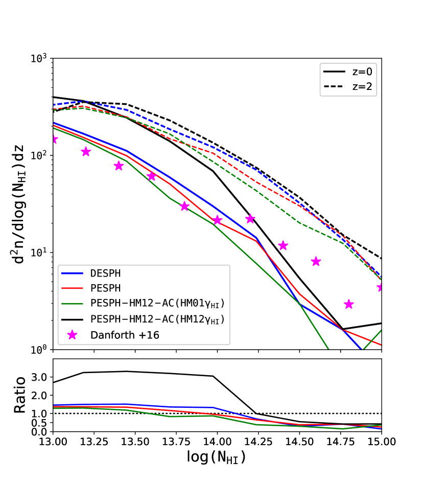
Figure 12: The upper panel compares the column density distributions (CDDs) for Ly$\alpha$ at $z=0$ and $z=2$. Blue and red lines present the CDDs from the DESPH and PESPH simulation with the HM01 background. The black lines show the CDD from the fiducial PESPH-HM12-AC with the HM12 background. Lastly, we recalculate the CDD for this run using the HM01 background for comparison (green lines). The $z=0$, and $z=2$ CDDs are plotted as dashed and solid lines, respectively. The turnover at $N_{HI}\sim 10^{13}\ \mathrm{cm^{-2}}$ shows the incompleteness in recovering under resolved lines assuming COS instrumental S/N and resolution. Data from Danforth et al. (2016) are plotted as magenta stars. The lower panel shows the ratio between the measured CDD at $z=0$ from simulations and the Danforth et al. (2016) data.

Figure 12 compares the HI column density distributions derived from Ly$\alpha$ absorbers at $z=0$ and $z=2$. We plot $d^{2}n/(d\log(N)dz)$ for better readability. The column densities are obtained from fitting Voigt profiles to all Ly$\alpha$ lines identified by AUTOVP over 70 random lines of sight that have an equivalent width broader than $0.03\AA$ within the redshift ranges $z=0-0.2$ and $z=1.8-2.0$, covering a total $\Delta z=14$. Qualitatively all four simulations show similar CDDs at both redshifts.

All three simulations (DESPH, PESPH, PESPH-HM01-AC) that use the same UV background (HM01) produce similar HI column density distributions at both redshifts, suggesting that the Ly$\alpha$ statistics are robust to different SPH schemes, despite the fact that hydrodynamical instabilities are much better captured in the new code. This is consistent with previous results that the baryonic structures are largely unaffected by the numerics. In detail, the PESPH-HM12-AC using the HM01 background yields a slightly lower CDDs at both redshifts. However, comparing the black line and the green line for $z=0$ indicates that changing the background from HM01 to HM12 increases the number density of low column HI absorbers by roughly 0.5 dex.

Our result supports the claim that the photoionisation rate derived in HM12 is insufficient to explain the abundance of low redshift HI absorbers (Kollmeier et al., 2014). We compare our derived CDDs to the new observational constraints from the HST/COS survey (Danforth et al., 2016) and find that the new fiducial simulation PESPH-HM12-AC still overproduces HI absorbers by a factor of 3 at low column densities. In order to match the observed distribution at $z=0$, we need to artificially boost the UV flux by a factor of $\sim 5$, a value that is consistent with Kollmeier et al. (2014). However, if we apply the HM01 background in our post-processing measurement, the CDD is very close to those from the DESPH and PESPH simulations. Therefore, the updated UV background is solely responsible for the enhancement of HI absorption in the our new fiducial simulation. Neither the SPH formulation nor the new cooling model has a strong impact on the Ly$\alpha$ statistics.

6.2 Metals

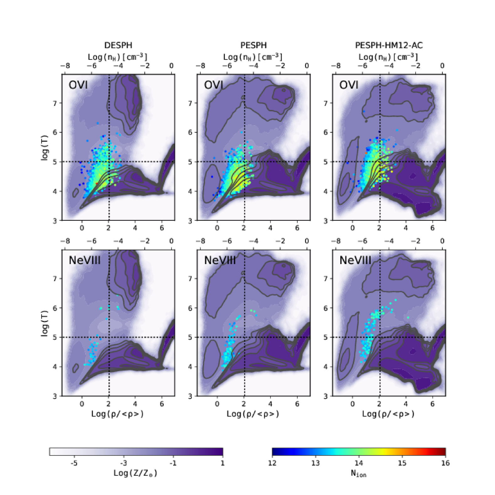
Figure 13: From left to right, the metal distribution in the density-temperature plane from the DESPH, PESPH and PESPH-HM12-AC simulations. The purple colour scale indicates the mass weighted average metallicity compared to solar. The solid lines divide the gas into four phases as defined for Figures 10 and 11. Over plotted dots represent OVI (upper panels) and NeVIII (lower panels) absorbers identified from $z=0$ to $z=0.5$ from 70 sightlines. The colour scale, which is identical in all panels, indicates the column densities of these absorbers, spanning from $10^{12}\ \mathrm{cm^{-2}}$ to $10^{16}\ \mathrm{cm^{-2}}$. The strong absorbers (redder in colour) have been stacked on top of weaker absorbers. Several contours lines are stressed for better visualisation.

Figure 13 compares the distribution of enriched gas in density-temperature phase space. The density and temperature dependence of metallicity is closely related to the outflows and encodes information of how outflows heat and enrich the gas in various phases. Though the metals locked within galaxies barely differ between simulations (see Figure 25 in Appendix E), the metal distributions in the gas phases are distinct. Specifically, the WHIM gas is more metal enriched in both the PESPH and PESPH-HM12-AC simulations, and the metals in the cool, condensed gas are more extended towards the hotter, less dense region. Satellite galaxies that enter hot haloes are more vulnerable to disruption owing to the enhanced hydrodynamical instabilities and mixing efficiency between fluid interfaces. In addition, shocks around filaments are better resolved, making more WHIM, metal rich gas. Furthermore, galactic winds are enhanced in massive galaxies in the PESPH simulation, further facilitating the mixture of enriched gas and metal-poor gas.

To compare the physical conditions from which observed absorption arises, we show the locations of OVI and NeVIII absorbers that we have studied previously (e.g., Oppenheimer et al., 2012) in the phase diagram. Most OVI absorbers still reside in diffuse gas where photoionisation dominates. The improved hydrodynamics leads to an increased number of strong absorbers in the condensed gas, in which the metal content now has a broader distribution. Similarly, there are more NeVIII absorbers in the PESPH and the PESPH-HM12-AC simulations, owing to higher metallicity in the warm gas.

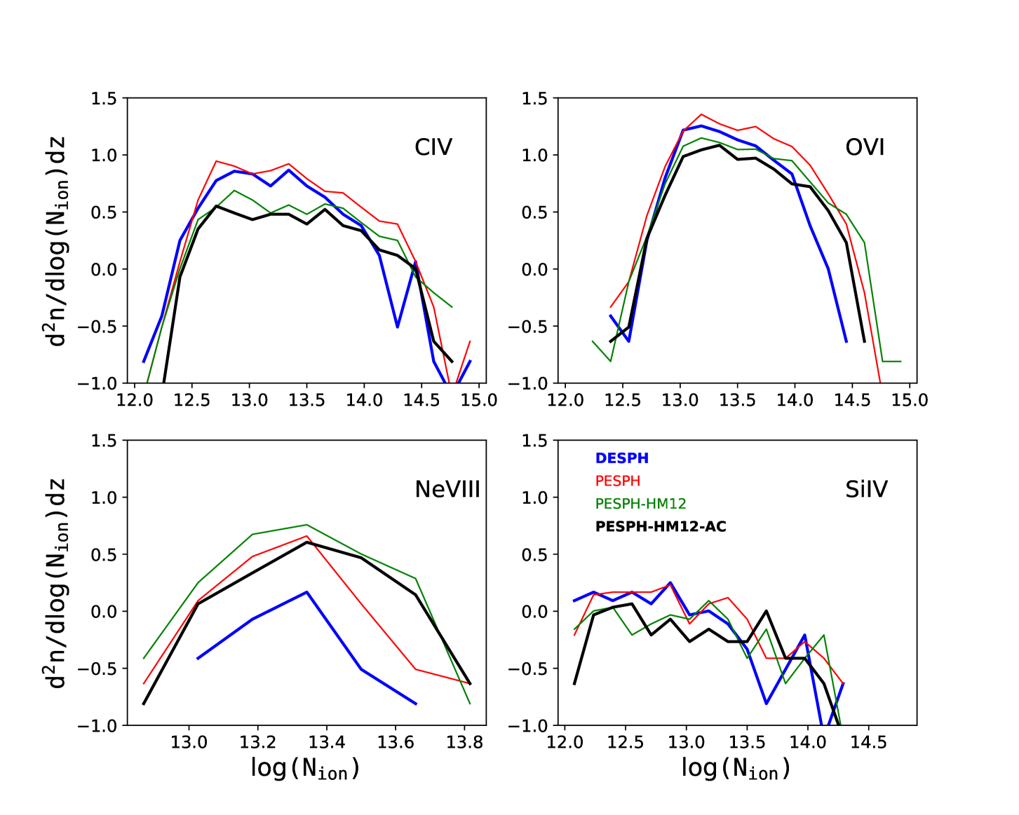
Figure 14: Comparison of the column density distributions of CIV, OVI, SiIV and NeVIII as labelled. Blue, red, green and black lines represent the CDDs from the DESPH, PESPH, PESPH-HM12 and PESPH-HM12-AC simulations, respectively. Nearby components fitted by AUTOVP that are within 100 km/s are combined into systems whose column densities and equivalent widths are summed over each component.

The column densities for metal ions are obtained in a similar way as for HI, except that the spectral lines are sampled from a wider redshift range, from $z=0$ to $z=0.5$ for each ion. Figure 14 compares the CDDs of several metal ions and shows the differences between the simulations. Changing SPH formulation alone (PESPH) leads to more absorption for both OVI and NeVIII. Changing the cooling prescriptions and the background boosts NeVIII absorption even further. Adding the new Cullen-Dehnen viscosity somewhat increases the high column OVI and slightly reduces the low column NeVIII absorption. The most important change is the factor of $5\sim 10$ boost in the CDD of NeVIII absorbers between DESPH and our fiducial calculation, which implies much better prospects for detecting this high-ionisation line. As shown in Figure 13, the increase owes to more metals in hot haloes.

6.3 Absorption in haloes

The absorption line systems in the spectra of bright distant objects probe the internal structures within a gaseous halo and, therefore, provide important constraints on the galactic winds that change the chemical and thermodynamic structures of simulated haloes. In this section, we create mock observations of halo gas surrounding the simulated galaxies at $z=0.25$ and examine whether predictions such as those in Ford et al. (2013, 2016) are sensitive to the numerics.

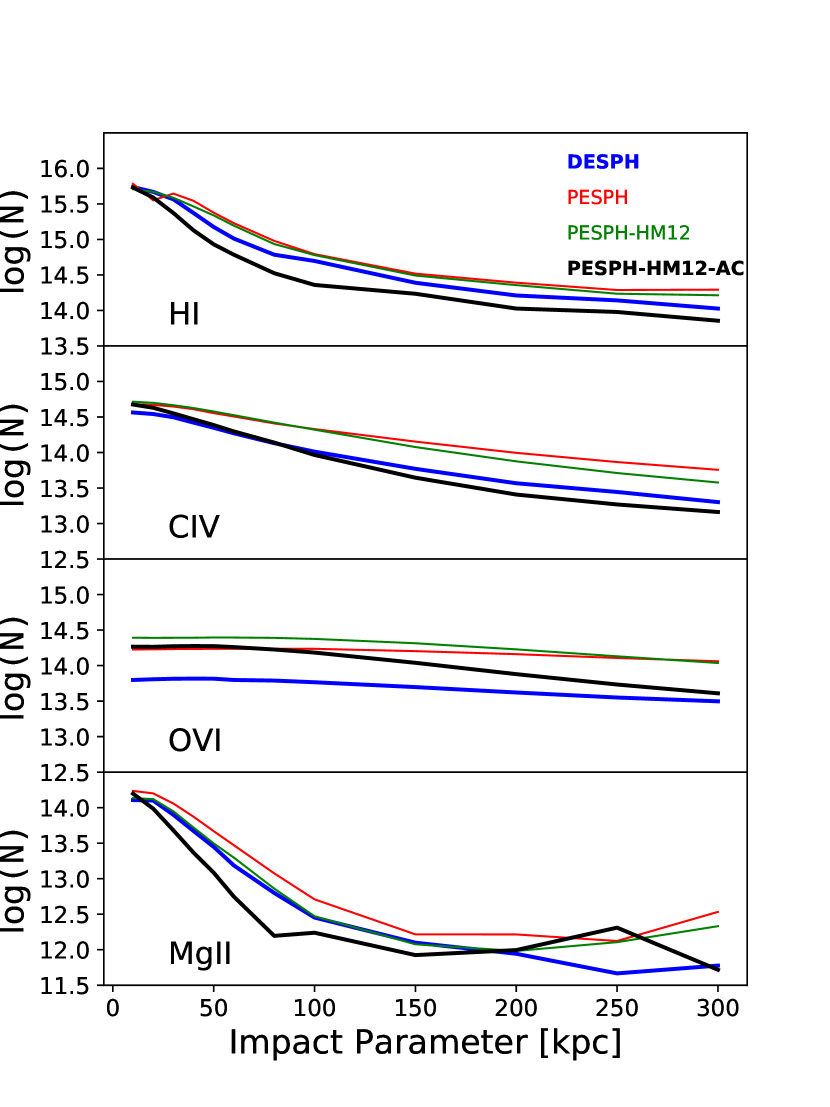
Figure 15: The averaged absorption profiles of 250 selected haloes from each simulation at $z=0.25$, with $11.75<\log(M_{h}/M_{\odot})<12.25$. The absorption is traced by the total column densities of several species as a function of impact parameter ranging from 10 kpc to 300 kpc. Blue, red, green and black lines show results from the DESPH, PESPH, PESPH-HM12 and PESPH-HM12-AC simulations, respectively.

Figure 15 shows the extension of absorption within $\log(M_{h}/M_{\odot})\sim 12$ haloes at $z=0.25$. At each impact parameter, we average over the column densities of all identified lines that are broader than $EW=0.03\ \mathrm{\AA}$ using over $\sim 1000$ lines of sight in 250 selected haloes. The $\log(M_{h}/M_{\odot})\sim 12$ haloes constitute a representative sample that is well resolved for studies of absorption. We choose upper limits of $10^{16}\ \mathrm{cm^{-2}}$ for HI and $10^{15}\ \mathrm{cm^{-2}}$ for other species. Column densities above these limits are reset to the limit value before being added. For MgII, the absorption drops dramatically within 100 kpc, while for ions with high ionisation potentials, such as CIV and OVI, the strength of absorption only mildly decreases as the impact parameter increases. The rise in MgII absorption at large radii is probably contamination by neighbouring galaxies.

Changing the SPH formulation to PESPH results in stronger absorption in all the species plotted here, with only a slight dependence on the impact parameter. The increase in the high ions such as CIV and OVI owes to more hot metals in the halo gas as shown in Figure 13. The absorption of HI within these massive haloes is more sensitive to the choice of SPH algorithm than we previously saw for the global HI column density distribution (Figure 12), indicating that the impact of the improved schemes is stronger within these massive haloes. Changing the cooling and UV background (PESPH-HM12) has little further effect except for MgII, which becomes smaller at all radii. However, switching to the new viscosity lowers the CIV at all impact parameters almost to the original DESPH values, and also reduces the OVI columns at large radii.

In summary, neither the new PESPH formulation nor the metal cooling model significantly changes our predictions for the global Lyman $\alpha$ statistics at z = 0 and z = 2. Using the HM12 background in post-processing calculations produces many more Lyman $\alpha$ absorbers in the column density range of $10^{13}\ \mathrm{cm^{-2}}<N_{HI}<10^{14}\ \mathrm{cm^{-2}}$, consistent with the findings from Kollmeier et al. (2014). The metal absorption line statistics are more sensitive to our algorithms. The PESPH formulation alone results in more CIV absorptions at $N_{CIV}>10^{13.5}\ \mathrm{cm^{-2}}$ and significantly more OVI and NeVIII absorbers at nearly all column densities. Adding the new metal cooling model does not further change the results, except for increasing the number of NeVIII detections even more.

6.4 X-ray galaxy groups

Both Fig.10 and Fig.13 have shown qualitative differences in the dense hot gas, which is closely related to X-ray emission. To study whether our predictions on the X-ray properties of galaxy groups (Davé et al., 2008; Liang et al., 2016) still hold, we derive X-ray luminosity weighted quantities following their method. The groups for this study are selected from the SO haloes that contain more than 8 SKID galaxies above the $6.0\times 10^{9}M_{\odot}$ baryonic mass resolution limit. First, we generate the X-ray spectrum for every SPH particle based on its density, temperature, metallicity and the local radiation background using the Astrophysical Plasma Emission Code (APEC) models (Smith et al., 2001). From each output X-ray spectra, we integrate the flux from 0.5 keV to 10 keV to get the X-ray luminosity for that SPH particle. Then we obtain for each halo the total X-ray luminosity by summing over all particles within the virial radius. We also obtain the X-ray luminosity weighted temperature and abundances of O and Fe by averaging over these particles. The emission weighting approximates the observational approach in which X-ray spectra are fitted with the APEC or other models to obtain temperature and abundances (Davé et al., 2008).

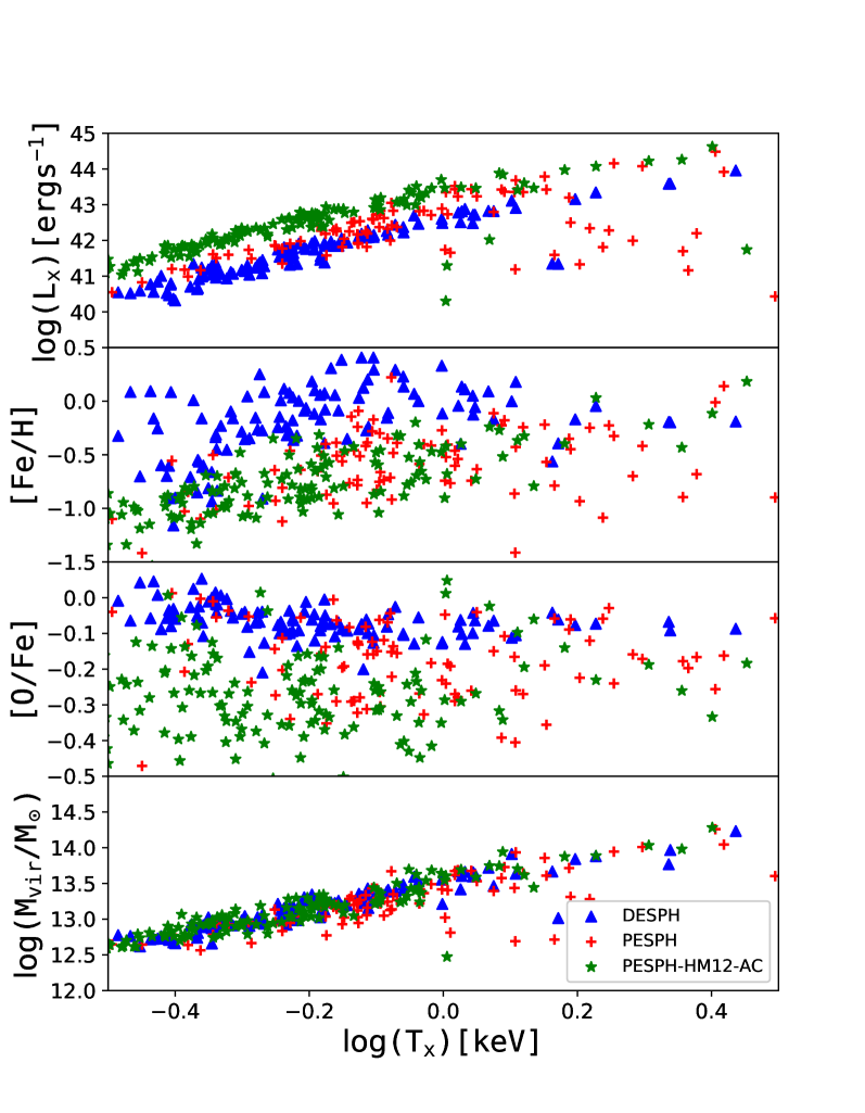
Figure 16: The dependence of X-ray luminosity weighted quantities of galaxy groups on their X-ray temperatures. Each point corresponds to a halo from each simulation that contains over 8 resolved galaxies. Haloes from the DESPH, PESPH and PESPH-HM12-AC simulations are plotted as blue triangles, red crosses and green stars, respectively. From the top to the bottom, the total X-ray luminosity $L_{x}$, iron abundance, alpha enhancement and the $M_{vir}$ of each individual group are plotted against its X-ray weighted temperature $T_{x}$.

Fig.16 compares how the various X-ray properties depend on the X-ray weighted temperature $T_{x}$ in our group sample. The bottom panel shows all three simulations agree well on the relation between $M_{vir}$ and $T_{x}$, but there are large differences in other X-ray properties. The upper panel shows the correlation between the total X-ray luminosity $L_{x}$ and $T_{x}$. Gravitational heating alone produces a scaling with $L_{x}\propto T_{x}^{2}$. However, a steeper relation has been observed for clusters and groups (White et al., 1997; Xue & Wu, 2000). The star formation and feedback processes that add non-gravitational energy into the ICM are supposed to alter the relation. This relation, therefore, helps us understand non-gravitational energy sources in our simulations. In this work, a power law scaling is reproduced in every simulation, but the normalisation and scatter vary. In particular, the $L_{x}$ of the PESPH-HM12-AC groups are systematically higher than the other simulations at fixed $T_{x}$ by $\sim$ 1 dex. This is likely related to the trend seen in the phase diagram (Fig.10) that the X-ray emitting gas in the PESPH-HM12-AC simulation is relatively cooler but much denser than in the DESPH simulation. In the PESPH simulation, some massive groups have $L_{x}$ that is much below the scaling relation. These groups also show much lower enrichment levels than other groups as seen in the next two panels.

The second and third panels of Fig.16 compare the X-ray luminosity weighted iron abundance [Fe/H] and the $\alpha$ element enhancement [O/Fe] as a function of $T_{x}$ for selected groups. Both the PESPH and the PESPH-HM12-AC groups have much lower $L_{x}$ weighted metals than the DESPH simulation and also have much larger scatters in these abundances at fixed $T_{x}$. To help us understand what causes the differences, we calculate [Fe/H] and [O/Fe] using mass-weighted and density-weighted abundances and compare the results from the DESPH and the PESPH-HM12-AC simulations in Fig.17. The mass-weighted [Fe/H] are significantly lower than the flux-weighted values in both simulations, because the flux-weighted abundances are dominated by the densest gas near the group centre, which is also most enriched (see the metal distributions shown in Fig.13). The differences between the flux-weighted abundances seen in the upper panels also disappear in the middle panels after the abundances are re-evaluated and weighted by mass, indicating that the discrepancies mostly owe to the different physical conditions of the densest gas. In the bottom panels, we compare the density-weighted abundances. The distribution of PESPH-HM12-AC groups on this diagram is nearly identical to the upper panels that use flux-weighted abundances. The groups in the DESPH simulation, on the other hand, still have much lower [Fe/H] compared to the flux weighted values, but their [O/Fe] ratios are quite similar now.

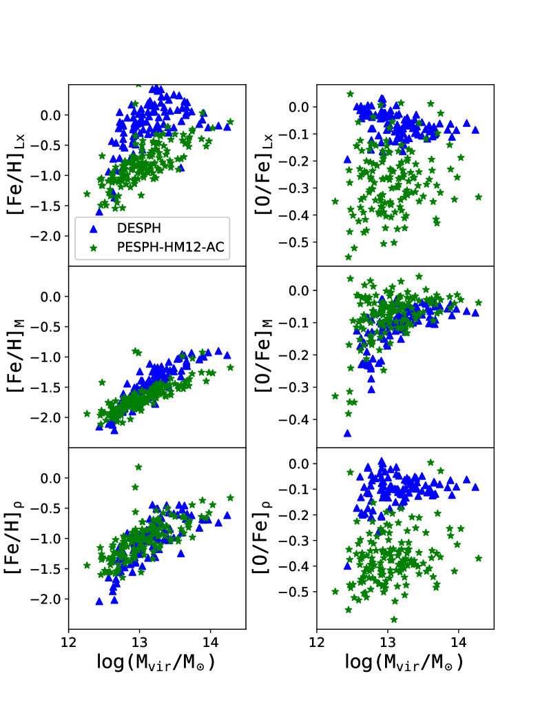
Figure 17: Iron abundances [Fe/H] (left panels) and $\alpha$ enhancements [O/Fe] (right panels) of individual groups as a function of their virial mass $M_{vir}$. The abundances are averaged over all hot gas within the virial radius but are weighted by $L_{x}$ (top panels), mass (middle panels) and density (bottom panels). In each panel we compare the results from the DESPH simulation (blue triangles) and the PESPH-HM12-AC simulation (green stars).

In summary, the X-ray properties of galaxy groups change significantly after improving the SPH formulation, artificial viscosity and the timestep regime. These abundances are very sensitive to the enrichment of the hot and dense gas, which is on average lower in simulations that use the PESPH formulation. This result suggests that numerical effects need to be taken into account when making predictions for the X-ray properties of groups and clusters.

7 SUMMARY

Cosmological baryonic simulations are important for understanding galaxy formation and evolution. SPH evolves the fluid equations by treating finite volume fluid elements as particles. The particle-based nature of SPH allows it to probe a large volume while maintaining high resolution at the smallest scales, and thus makes it suitable for simulations in a cosmological context. However, traditional SPH has difficulties resolving gas dynamics in subsonic flows, namely it suppresses instabilities and prevents multi-phase mixing. Hopkins (2013) posed an alternative form of the SPH equations of motion that eliminates these problems. We implemented the new formalism into our GADGET-3 code, along with improved treatments of the artificial viscosity and the timestep criteria. We performed standard fluid tests as well as full cosmological tests in a co-moving volume to test the new algorithm. We also update our metal line cooling model to include non-CIE effects in the presence of the Haardt & Madau (2012) UV background. The HM12 background is a more up-to-date estimate of the background flux using a more careful assessment of galaxy and quasar contributions as a function of time. The Wiersma et al. (2009) cooling model considers the extra cooling owing to free electrons from metals, which is potentially significant in neutral gas.

In this work, we focus on studying the impact of these improvements in both numerical algorithms and physics to simulations within a cosmological context. The main conclusion is that the majority of observables we have studied in previous work (Oppenheimer & Davé, 2008; Finlator & Davé, 2008; Oppenheimer et al., 2010; Peeples et al., 2010a, b; Davé et al., 2011a, b; Oppenheimer et al., 2012; Davé et al., 2013; Kollmeier et al., 2014; Ford et al., 2016), whether on global scales or galactic/halo scales, are not significantly affected by either the new hydrodynamical models or the cooling model, while at the same time, the unphysical clumping of cold gas owing to the deficiencies of the original algorithms is effectively removed. However, observables related to the amount or metallicity of hot gas are affected.

We do not extensively explore how the differences caused by the different SPH schemes will be affected by numerical resolution, but the effect of a modest increase in resolution such as in a zoom-in simulation is likely to be unimportant. The standard hydrodynamic tests, in which the differences caused by different numerical algorithms are distinct, have much higher resolution than even the zoom-in simulations. The major difference between the DESPH and the PESPH is the efficiency of phase mixing, which is intrinsic to the SPH formulation and independent of resolution. Hopkins et al. (2018) discuss the effects of SPH implementations in the zoom-in, Feedback in Realistic Environments (FIRE) simulations. They find that many of their qualitative conclusions are robust to SPH implementations, but the efficiency of phase mixing has important effects on CGM properties and subsequent cooling and re-accretion of the CGM gas in massive, hot halos. This general conclusion is consistent with our findings from lower resolution simulations on cosmological scales.

The cosmological simulations in this work do not include AGN feedback, nor did our previous simulations. Therefore, we do not assess the impact of different SPH schemes on AGN feedback in this work. Schaller et al. (2015) demonstrate that the pressure-entropy SPH enhances phase mixing between accreted gas and the AGN driven bubble and, therefore, affects the efficiency of AGN quenching. This leads to changes in the stellar mass content and the X-ray emission from the intragroup medium in massive halos. However, this effect of changing numerical schemes likely depends on the resolution and could be mitigated with a recalibration of the subgrid parameters that govern the efficiency of the AGN feedback. The nIFTy comparison project also demonstrates that a variety of simulations, which employ a variety of different numerical and feedback models, produce similar gas properties for a galaxy cluster (Sembolini et al., 2016b), even though the different numerical schemes without the subgrid models lead to significant differences in the gas profiles of the simulated clusters (Sembolini et al., 2016a). This further indicates the importance of subgrid models and their calibration.

We conclude:

1. The PESPH formulation alone significantly enhances hot mode accretion in massive haloes at all redshifts, indicating that cooling is more efficient in these systems, and that some cold mode accretion is transformed into hot mode accretion owing to better resolved shocks. In the simulations that employ momentum-driven wind feedback, cold mode accretion and wind reaccretion still dominates at early and late times, respectively, regardless of the numerical scheme used. The total amount of accretion only slightly increases owing to more efficient wind reaccretion at lower redshifts. The impact of the PESPH formulation is much stronger in the nw simulations where wind-reaccretion is not present. The hot accretion fraction increases substantially at most redshifts and especially at high redshifts, where it becomes dominant in $\log(M_{h}/M_{\odot})>11$ haloes. Consistent with our previous work, cold mode accretion dominates the overall growth of the galaxy population at high redshift and the growth in low mass haloes at low redshift, while wind re-accretion dominates galaxy growth in massive haloes at $z<2$.

   Nelson et al. (2013) investigates the gas accretion problem using a set of non-feedback cosmological simulations simulated with the moving mesh code AREPO. Using a similar temperature cut to distinguish cold and hot mode accretion, they find the cold mode accretion is nearly completely removed from $z=2$ haloes with $\log(M_{h}/M_{\odot})\sim 12$. In our simulations, however, despite the fact that the cold accretion fraction significantly drops owing to the PESPH formulation, it is still present at the $\sim 20\%$ level in most haloes at $z=2$. This disagreement is not likely caused by the artificial clumps seen in DESPH simulations, since the PESPH formulation has eliminated these features and yet is still able to fuel central galaxies of the massive haloes with cold gas. However, a detailed comparison with their work is not feasible owing to both the different sub-grid assumptions and the accretion tracking method.

2. The PESPH formulation, along with the Cullen & Dehnen (2010) viscosity and the Durier & Dalla Vecchia (2012) timestep criteria enhances the star formation rate in our fiducial ezw model by as much as 20% after the star formation peak at $z\sim 3$, increasing the number density of massive galaxies at low redshifts. The non-CIE cooling model suppresses cooling and star formation by a comparable amount after the star formation epoch, resulting in a SFH close to the original one. The enhanced star formation in massive systems owing to numerical improvements, however, is much smaller than the discrepancies between the simulations and observations. The requirement of additional feedback, either AGN or a different supernova feedback algorithm (Huang et al in prep.) that quenches star formation in massive galaxies is not alleviated. Moreover, as pointed out by Hu et al. (2014), the impacts of PESPH and artificial viscosity on star formation and feedback probably depends on the feedback implementation. In the thermal feedback scheme, the mass loading is significantly reduced by the enhanced mixing between SNe heated gas and the surrounding cool gas, while our kinetic feedback is much less sensitive to the efficiency of mixing.

3. Using the fiducial PESPH-HM12-AC simulation that employs the state-of-art numerical algorithms, we confirm the “photon underproduction crisis” reported in Kollmeier et al. (2014). Namely, our simulation strongly overproduces the column density distributions of HI absorbers at low redshift if we adopt a uniform HM12 ionisation background. We find that the HI column density distribution traced by Ly$\alpha$ absorption is very robust to the choices of hydrodynamics. However, changing from the HM01 background to the HM12 background boosts the amount of HI absorbers by a factor of 3, which is consistent with the findings from Kollmeier et al. (2014). The conclusion that the predicted Ly$\alpha$ forest is robust to hydrodynamics is also reported in Gurvich et al. (2016), who shows that the differences between a traditional SPH (DESPH) code and the moving mesh code are small in the low column density range studied here.

4. The distributions of baryons in the density-temperature phase diagram are quite similar in general, with the exception that the PESPH formulation leads to more hot gas at higher densities, and the non-CIE metal cooling model results in a larger scatter in the condensed gas phase. The mass fractions of baryons that reside in the various phases: diffuse, WHIM, hot, condensed, and stars, are surprisingly similar in all simulations at most redshifts. The hot gas fraction in galaxy groups is enhanced by a small amount in the wind models compared to the ones without galactic winds, indicating that the contribution of galactic winds to the hot intragroup medium is small. In spite of the different feedback models, the amount of hot gas is quite robust to the numerical schemes.

5. The PESPH formulation enhances metallicity in the WHIM and hot halo gas. As a result, the PESPH simulations generally produces more absorbers for some of the high ions, e.g., CIV, OVI, NeVIII, SiIV, on both global scales indicated from their column density distributions and within $\log(M_{h}/M_{\odot})=12$ haloes at low redshift. The non-CIE cooling and the HM12 background reduce the amount of weak absorption, except for NeVIII absorption, which is even further enhanced by these changes at all column densities.

6. The X-ray group properties change significantly with the improvements in the hydrodynamics, but they are insensitive to the adopted cooling model. The X-ray luminosity weighted iron abundance and $\alpha$ enhancement in the group sample are both greatly reduced and have much larger scatter in the PESPH and PESPH-HM12 simulations compared to original results from the DESPH simulation. These differences mostly owe to the different metallicities in the densest gas near the group centre in these simulations. There are also more outliers from the $L_{x}-T_{x}$ scaling relation, which correspond to groups that have the lowest X-ray weighted metallicity. A more careful analysis of X-ray properties is left for future work.

7. In Appendices C, D and E, we show that the change from our previous DESPH formulation to the new PESPH-HM12-AC prescription has little impact on many of the key characteristics of galaxy evolution: star formation histories as a function of halo mass, the HI mass function, and the redshift-dependent scaling relations between galaxy stellar mass and specific star formation rate, cold gas fraction, and gas phase metallicity. These characteristics and many of the others mentioned above can, therefore, be used to set constraints on the physics of stellar and AGN feedback, galactic outflows, and metal mixing in the CGM, without high sensitivity to numerical or microphysical uncertainties.

In summary, we test the PESPH formulation, along with other improved numerical technologies and physical models, in full cosmological hydrodynamic simulations that are implemented with state-of-art models for baryonic physics. The new implementations successfully removed long standing numerical artefacts without significantly affecting most predictions from previous simulations.

Appendix A The Sedov-Taylor Blastwave Test

The Sedov-Taylor blast wave test starts with a point explosion within a uniform medium that creates a strong shock wave, which sweeps through its surroundings. The numerical solution to this problem is very sensitive to the shock capturing capabilities owing to the sharp entropy discontinuity at the shock front. In SPH, shocks are captured by numerical dissipation through artificial viscosity. Therefore, this problem is a strong test of the artificial viscosity scheme and the viscosity parameters. We set up a three dimensional uniform lattice in a $6^{3}\ \mathrm{kpc}^{3}$ cube with 64 particles on a side. The volume has a uniform initial density of $1.24\times 10^{7}M_{\odot}\ \mathrm{kpc}^{-3}$ and temperature of $10\ K$. We start the simulation by injecting $E=6.78\times 10^{53}$ ergs of energy into the eight central particles, resulting in a initial entropy contrast of $3\times 10^{6}$ and a Mach number of $\sim 1000$.

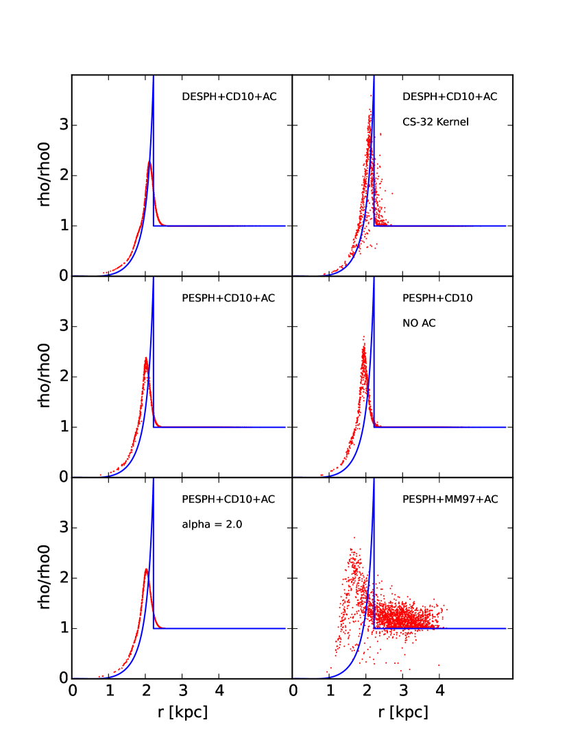
Figure 18: Numerical solutions of the Sedov-Taylor blastwave tests are compared to the analytic solution. The analytic solution for the overdensity as a function of radius from the energy injection point is shown in blue. In each panel, each red dot represents an SPH particle from the simulation. One out of a thousand particles are displayed here. The first row uses the DESPH formulation in addition to the Cullen & Dehnen (2010) viscosity and artificial conduction with our fiducial parameters. The right panel of the first row uses the old cubic spline kernel instead of our fiducial quintic kernel. The other four panels use the PESPH formulation with different choices of viscosity and conduction: In the second row, the left panel is the fiducial numerical choice for our cosmological simulations; the right panel does not have the artificial conduction. In the third row, the left panel uses $\alpha_{max}=2.0$ for the viscosity, larger than our fiducial $\alpha_{max}=1.5$ value; the right panel uses the Morris & Monaghan (1997) viscosity with the $\alpha_{i}$ starting from the minimum value $\alpha_{min}=0.2$.

The Figure 18 shows the results from six simulations. We find that to reach a good agreement between the numerical result and the analytical solution for the Sedov-Taylor test, a higher order kernel with a large enough number of neighbours, combined with a timestep limiter and a sensitive artificial viscosity switch are crucial. Simulations that incorporate these features reproduce the analytic solution reasonably well. The shock fronts align with each other, although the numerical solutions have a reduced peak density and some post-shock ringing effects.

The PESPH formulation performs worse than the DESPH formulation, because the entropy-weighting nature of PESPH exaggerates noise at the entropy jump, which is very sharp in this test, as is also found in other work (Hu et al., 2014; Read & Hayfield, 2012). Also, the shock fronts in PESPH simulations are delayed compared to the analytic solution, a phenomenon also shown in Read & Hayfield (2012) with their RT formulation, which similarly evaluates the density using entropy weighting.

The Morris & Monaghan (1997) viscosity (bottom right panel) is very poor at shock capturing. Note that in this test, the $\alpha$ parameters of the particles start from the minimum value as in the cosmological simulations where the viscosity is applied. The density profile is very noisy at the shock front and particle penetration is evident. Those particles in the shock are not sufficiently shocked owing to the slowly-growing $\alpha$. Since the energy injection is not isotropic, particles that lie in the direction of the energy injection propagate much further than the surrounding particles. The Cullen & Dehnen (2010) viscosity, on the other hand, prepares these particles by boosting the $\alpha$ parameter to the maximum value even before the shock front passes and thus effectively captures the shock. Our fiducial choice of $\alpha_{max}=1.5$ is a compromise between efficient shock capturing and lowering unwanted dissipation. The bottom left panel shows the results using a slightly larger $\alpha_{max}=2.0$, but the improvement is only marginal.

The choice of kernel is not trivial in this test. A low order cubic spline kernel with 32 neighbours, even in an idealised case with DESPH, Cullen & Dehnen (2010) viscosity, and artificial conduction, still produces a lot of noise at the shock front (top right panel). This is also similar to Read & Hayfield (2012), where they found a cubic spline kernel with 42 neighbours results in a much more noisy shock front than a higher order HOCT kernel with 442 neighbours, despite the fact that the HOCT kernel lowers the spatial resolution by a factor of 1.5.

Artificial conduction reduces the noise at the shock front by smoothing the entropy contrast. It can be effective in reducing noise within the PESPH formulation, but the effect is not significant in our tests. Note that our artificial conduction coefficient is only one quarter of the commonly adopted value.

Finally, we need to emphasise that all the simulations above use the timestep limiter that adjusts the timesteps of particles in the vicinity of large energy fluctuations, so that these particles are able to react to the approaching shock in time. We use a Courant factor of 0.05 to determine the timesteps in general. However, without the timestep limiter, the results degrade significantly.

Appendix B Artificial Conduction in a Cosmological Volume

Artificial conduction is introduced as a pure numerical tool whose purpose is to smooth out fluid discontinuities in some high resolution standard test problems and thus to achieve realistic solutions to these problems. However, in a large cosmological volume, such high resolution is unattainable. Moreover, artificial conduction could lead to spurious cooling near galaxies and compromise the validity of the results. Since the radiative cooling rate depends critically on the gas temperature especially at the disc-halo interface, non-linear effects could magnify the effects of conduction on gas cooling. In this section, we investigate the role of artificial conductive cooling in our cosmological tests and compare it to the amount of radiative cooling.

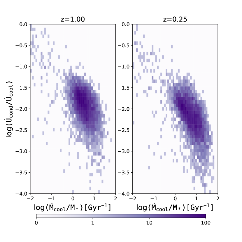
Figure 19: The cooling ratios between artificial conductive cooling and net cooling (including conductive cooling and heating sources) are plotted against the specific net cooling rate for each halo from the PESPH-HM12-AC simulation. Results at $z=1$ and $z=0.25$ are shown in the left and right panels, respectively. Here radiative cooling is computed only from non-SF particles. Note that the net cooling rate $\dot{U}_{cool}$ includes all cooling and heating sources, so the ratio can be large where cooling balances heating so that the net cooling rate is small. In GADGET-3, it is not straightforward to separate the radiative cooling rate from the net cooling rate, so it is hard to directly compare conductive cooling to radiative cooling.

We take snapshots at $z=1$ and $z=0.25$ from our fiducial PESPH-HM12-AC simulation and measure the cooling rates in all the SO haloes identified in each snapshot. Figure 19 compares the ratio between the total conductive cooling rate $\dot{U}_{cond}=\sum_{i}m_{i}\dot{u}_{cond,i}$ and the total net cooling rate $\dot{U}_{cool}=\sum_{i}m_{i}\dot{u}_{cool,i}$ in each halo, as a function of the specific cooling rate, defined as $\lambda_{cool}\equiv\dot{M}_{cool}/M_{*}$, where $M_{*}$ is the stellar mass of the central galaxy, and $\dot{M}_{cool}\equiv\sum_{i}m_{i}\dot{u}_{cool,i}/u_{i}$.

Conductive cooling is almost always small and sub-dominant compared to the net cooling. In a few haloes, where the ratio $\dot{U}_{cond}/\dot{U}_{cool}$ approaches unity, the specific cooling rates are too small to be important to the thermal histories of these haloes. In haloes where conductive cooling is fast, the net cooling is orders of magnitude faster, making the contribution from artificial conduction negligible.

There are elements in our conduction scheme that attempt to restrain conduction to only fluid discontinuities. Our requirement that conduction occurs only when the signal velocity between particles, $v_{sig}=c_{i}+c_{j}-3\omega_{ij}$, is positive suppresses conduction in non-converging flows. Also, the factor $L_{ij}$ reduces conduction in pressure equilibrium. The artificial conduction coefficient that we use ($\alpha_{cond}=0.25$) is only one quarter of the commonly assumed value, but increasing conduction by a factor of 4 does not significantly alter the results above. We did not specifically study the heating from conduction. The artificial conduction scheme that we adopt is conservative so that the amount of conductive heating is equal to the conductive cooling. The cool gas will thus quickly dissipate the heat gained from conduction and return to thermal equilibrium on a very small time-scale. Therefore, we are confident from these tests that the spurious numerical dissipation from our implementation of artificial conduction has a minimal effect on the growth and evolution of galaxies in a cosmological volume.

Appendix C Star Formation Histories

In previous sections we have shown that the accretion rate, total stellar content, and the stellar mass function are barely affected by the improved numerics. Here we examine the star formation histories (SFH) from our simulations and how they are affected by the numerics. The SFH reflects the overall efficiency of galaxy formation and relies on critical processes such as accretion efficiency, cooling, and feedback.

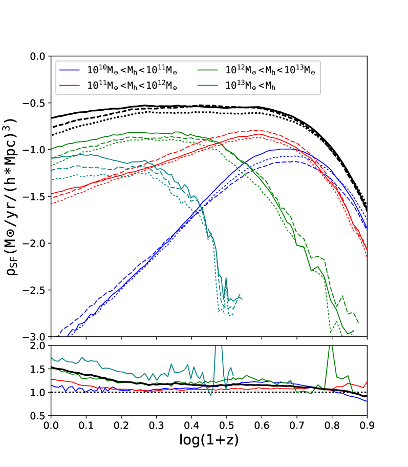
Figure 20: The upper panel shows the star formation histories of three simulations with galactic winds (ezw). The dotted, dashed and solid lines correspond to the DESPH, PESPH, and PESPH-HM12-AC, respectively. The black lines show the global star formation density as a function of redshift. The blue, red, green and teal lines show the summed star formation density at any time from individual haloes grouped according to their total mass $M_{h}$ at that redshift as labelled. The bottom panel shows the ratios of the SFRDs from the PESPH-HM12-AC and the DESPH simulations for each halo mass bin, using the same colour scheme.

Figure 20 presents the global SFH of the DESPH, PESPH, and PESPH-HM12-AC simulations. We plot the contribution to the star formation rate from haloes that are grouped by their total mass. At each redshift, the SFR of each ISM particle is computed based on the subgrid SF model, then the SFR of each halo is summed over all the ISM particles that it contains. We have included contributions from sub-resolution galaxies since we are focusing here on the total amount of baryons in stars and the effect of including these galaxies is actually small.

The overall evolution of the star formation histories is similar in the three simulations. All SFHs are characterised by a sharp peak at $z\sim 3$ and a gradual decline afterwards. The total SFHs in the DESPH and PESPH runs agree quite well before the star formation epoch, then the PESPH starts to form $\sim 20\%$ more stars than the DESPH all the way down to $z=0$. This offset is caused only by the different treatment of hydrodynamics. Massive haloes with $\log(M_{h}/M_{\odot})>11$ in the PESPH simulation form stars at a higher rate over the entire time, causing the overall $20\%$ more stars after $z\sim 3$.

Compared to the PESPH results, the new cooling model and background in the PESPH-HM12-AC simulation suppresses star formation in all haloes after the star formation peak, but has little effect at higher redshift. In the Wiersma et al. (2009) cooling model, species that dominate cooling in warm gas are over ionised relative to collisional equilibrium in the presence of the photoionising background, shifting their cooling curves toward lower temperature, suppressing the net metal-line cooling efficiency and the star formation rate. Therefore, the differences between PESPH and PESPH-HM12-AC are primarily caused by the cooling models used.

Coincidentally, our implementation of hydrodynamics and physics works against each other in regulating the star formation processes. The combined effects produce a star formation history that closely resembles the results from our previous model, except for a short period of slightly enhanced star formation between $z=2$ and $z=3$. It is clear from the bottom panel that the massive haloes at these redshifts contribute most to the overall enhanced star formation.

Appendix D HI Mass Function

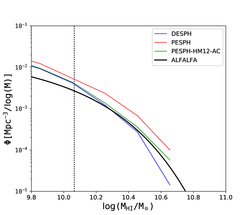
Figure 21: The neutral hydrogen mass functions (HIMFs) at $z=0$. Blue, red and green lines represent results from the DESPH, PESPH and PESPH-HM12-AC simulations, respectively. We also include the Schechter fit of the HIMF from the $\alpha.40$ sample of ALFALFA survey (Haynes et al., 2011) as thick black solid line. The vertical dotted line indicates the stellar mass resolution limit, which is comparable to the neutral hydrogen mass limit (Davé et al., 2013).

Figure 21 compares the neutral hydrogen mass functions (HIMFs) from our simulations. We calculate the neutral hydrogen fraction of every gas particle following Davé et al. (2013). In summary, we first calculate the optically thin limit of the neutral fraction by solving for ionisation equilibrium based on local density, temperature and the radiation field. Then the column density is integrated for each gas particle, assuming a uniform distribution of neutral hydrogen within a sphere with a radius equal to its smoothing length. If the column density of HI calculated as such exceeds a threshold of $N_{HI,lim}=10^{17.2}\ \mathrm{cm^{-2}}$ where the gas becomes optically thick, we compute the HI content by including the self-shielding of neutral hydrogen, and compute the fraction of the molecular hydrogen component by using the observed pressure relation (Leroy et al., 2008). The HI mass of each galaxy is summed over all gas particles within a sphere that extends to the outermost radius of the galaxy.

The three simulations generally agree with each other. The galaxies from the PESPH simulation show slightly more neutral gas content than those from the DESPH simulation. Two comparable effects contribute to this small yet non-negligible discrepancy. First, the galaxies from the PESPH simulation assemble in slightly denser regions where the neutral fraction is higher. Second, the spherical region surrounding PESPH galaxies encloses more gas particles. Ram pressure stripping on resolved scales, which is supposed to be enhanced by PESPH, does not significantly lower the neutral gas content in satellite galaxies. Adding the improved physics decreases the HI masses almost back to their original DESPH values.

Appendix E sSFR, MZR and Gas Fraction

Observed galaxy populations often present tight scalings between various properties such as the star formation rate, metallicity, cold gas fraction and the stellar mass. These scaling relations result from a complicated interplay between physical processes that are critical to galaxy formation and evolution, and reproducing them has been a key test of cosmological simulations. In this section, we demonstrate that these properties of simulated galaxies are also robust to the different numerical models and physics explored in this work.

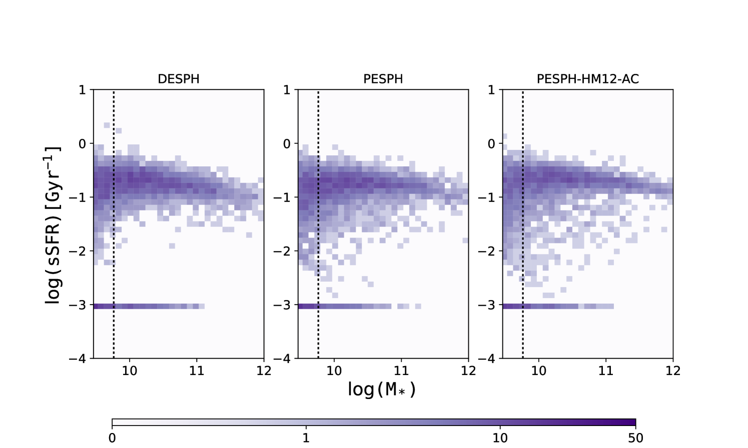
Figure 22: The specific star formation rates (sSFR) of simulated galaxies as a function of their stellar masses at $z=0$. The horizontally stretched region around sSFR $=10^{-3}\ \mathrm{Gyr}^{-1}$ is populated by galaxies that contain no gas (and hence no star formation), so we assign an arbitrary sSFR. The dotted vertical line indicates half the resolution limit (32 gas particles). The number density of galaxies in each bin is colour coded in purple.

Figure 22 compares the specific star formation rate as a function of stellar mass for individual galaxies from the simulations at $z=0$. We calculate the sSFR by averaging the star formation rates of all SPH particles with densities above the star forming threshold in each galaxy. There are also quiescent galaxies in our simulations that only contain star particles and no gas particles. We assign an arbitrary value of $sSFR=10^{-3}\ \mathrm{Gyr}^{-1}$ to these galaxies. The two PESPH simulations produce slightly more low sSFR galaxies, but the overall results of all these simulations are very similar. Cosmological simulations without feedback do not reproduce the observed red population of local galaxies (Kereš et al., 2009b), and the kinetic feedback model employed here with improved numerical schemes is still not able to resolve this discrepancy. This finding strengthens the conclusion that a new feedback scheme, possibly adding AGN feedback, is needed to explain the observed population of passive galaxies.

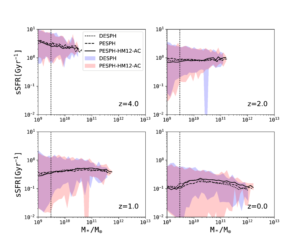
Figure 23: The relation between sSFR and stellar mass at four different redshifts. The dotted, dashed and solid lines are medians of the sample from the DESPH, PESPH and PESPH-HM12-AC simulations, respectively. The shaded area contains 95% of galaxies in each mass bin (representing only galaxies from DESPH and PESPH-HM12-AC). The dotted vertical line indicates half the resolution limit (32 gas particles).

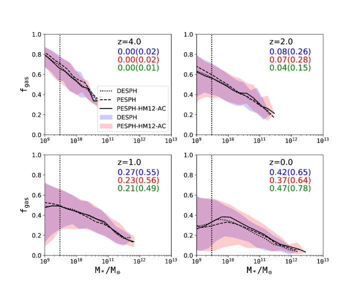
Figure 24: The relation between gas fraction and stellar mass at four redshifts. The dotted, dashed and solid lines are the medians of the sample from DESPH, PESPH and PESPH-HM12-AC simulations, respectively. Black lines include all galaxies while green lines only include satellite galaxies. The shaded area contains 95% of galaxies in each mass bin, including only the galaxies from the DESPH and PESPH. The dotted vertical line indicates half of the resolution limit (32 gas particles). The floating numbers in each panel indicate the fraction of gas-free galaxies in each simulation, with the number within the parentheses indicating the gas-free satellite galaxies.

The sSFR-$M_{*}$ relation also agrees very well between simulations at most redshifts (Figure 23). The shaded areas encloses 95% of the galaxies from each sample. Here we only compare the scatter of the relation from the DESPH and the PESPH-HM12-AC simulation to highlight the differences between our old and new fiducial runs. The scatter also agrees quite well between the old and new model at all redshifts, except that the new fiducial simulation PESPH-HM12-AC contains some galaxies with very low sSFR at $z=0$ and $z=1$.

The gas content within galaxies is balanced by accretion and gas consumption owing to star formation. Figure 24 shows the trend of gas fraction within galaxies with their stellar mass. The gas fraction $f_{gas}$ is defined to be the mass of all gas particles within a galaxy divided by the total mass. The galaxies that are not star forming have been excluded from this sample. The same trend that the gas content is on average lower in more massive galaxies is observed in all simulations. Moreover, both the medians and the distributions of the gas fractions at any particular stellar mass bin are very similar among the simulations. The regulation of the gas reservoir in individual galaxies is mostly affected by the star formation and feedback prescriptions, while the choice of hydrodynamical method and background appears to have little impact. Apart from the general agreement, the PESPH simulation has slightly more gas-free galaxies, but most of them are under resolved. These galaxies are not counted while drawing the median, but the effect of including them would be small. In addition, galaxies in the PESPH simulations have a slightly larger gas fraction in general than DESPH galaxies at all redshifts, as indicated both by the median and the shaded area. It suggests that the gas supply in PESPH galaxies must be generally more efficient at refilling their consumed gas to compensate for the higher star formation and outflow rate. This is consistent with our previous finding that PESPH galaxies have a higher overall accretion rate.

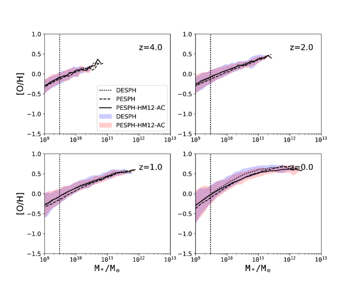
Figure 25: The stellar mass-gas metallicity relation at four redshifts. The metallicity is weighted by the star formation rate of all gas particles within each galaxy. The dotted, dashed and solid lines are the running medians of the sample for DESPH, PESPH and PESPH-HM12. The shaded area contains 95% of the galaxies in each mass bin, including only the galaxies from the DESPH and PESPH-HM12 simulations. The dotted vertical line indicates half the resolution limit (32 gas particles).

Figure 25 compares the mass-metallicity relation (MZR) at four redshifts. Our version of GADGET-3 traces the abundances of C, O, Si and Fe separately. Here we estimate the metallicity from the oxygen abundance normalised to the solar value, assuming a solar oxygen mass fraction of 0.009618 (Anders & Grevesse, 1989). The metallicity of each galaxy is averaged over all the ISM particles weighted by their star formation rate. This definition avoids a bias to gas particles lying in the outskirts of galaxies and mimics the observational approach of measuring metallicity (Davé et al., 2011b). The slope and scatter of the relation are both preserved by the PESPH and PESPH-HM12 simulations, while the metal content in both simulations decrease at all mass scales, most clearly seen at $z=0$, where the intergalactic gas metallicity generally drops by 0.1 dex. The new hydrodynamics that boosts star formation in massive galaxies facilitates metal enrichment as well, maintaining the shape of the relation, while the altered balance between inflow and outflow could have lowered the metal content.

References

- Abel (2011) Abel T., 2011, MNRAS, 413, 271
- Agertz et al. (2007) Agertz O., et al., 2007, MNRAS, 380, 963
- Anders & Grevesse (1989) Anders E., Grevesse N., 1989, Geochimica Cosmochimica Acta, 53, 197
- Balsara (1995) Balsara D. S., 1995, Journal of Computational Physics, 121, 357
- Barnes & Hut (1986) Barnes J., Hut P., 1986, Nature, 324, 446
- Berger & Colella (1989) Berger M. J., Colella P., 1989, Journal of Computational Physics, 82, 64
- Bryan et al. (2014) Bryan G. L., et al., 2014, ApJS, 211, 19
- Chabrier (2003) Chabrier G., 2003, PASP, 115, 763
- Cullen & Dehnen (2010) Cullen L., Dehnen W., 2010, MNRAS, 408, 669
- Dalla Vecchia & Schaye (2008) Dalla Vecchia C., Schaye J., 2008, MNRAS, 387, 1431
- Danforth et al. (2016) Danforth C. W., et al., 2016, ApJ, 817, 111
- Davé & Tripp (2001) Davé R., Tripp T. M., 2001, ApJ, 553, 528
- Davé et al. (1997) Davé R., Hernquist L., Weinberg D. H., Katz N., 1997, ApJ, 477, 21
- Davé et al. (2001) Davé R., et al., 2001, ApJ, 552, 473
- Davé et al. (2008) Davé R., Oppenheimer B. D., Sivanandam S., 2008, MNRAS, 391, 110
- Davé et al. (2010) Davé R., Oppenheimer B. D., Katz N., Kollmeier J. A., Weinberg D. H., 2010, MNRAS, 408, 2051
- Davé et al. (2011a) Davé R., Oppenheimer B. D., Finlator K., 2011a, MNRAS, 415, 11
- Davé et al. (2011b) Davé R., Finlator K., Oppenheimer B. D., 2011b, MNRAS, 416, 1354
- Davé et al. (2013) Davé R., Katz N., Oppenheimer B. D., Kollmeier J. A., Weinberg D. H., 2013, MNRAS, 434, 2645
- Davé et al. (2016) Davé R., Thompson R., Hopkins P. F., 2016, MNRAS, 462, 3265
- Dehnen & Aly (2012) Dehnen W., Aly H., 2012, MNRAS, 425, 1068
- Durier & Dalla Vecchia (2012) Durier F., Dalla Vecchia C., 2012, MNRAS, 419, 465
- Finlator & Davé (2008) Finlator K., Davé R., 2008, MNRAS, 385, 2181
- Finlator et al. (2006) Finlator K., Davé R., Papovich C., Hernquist L., 2006, ApJ, 639, 672
- Ford et al. (2013) Ford A. B., Oppenheimer B. D., Davé R., Katz N., Kollmeier J. A., Weinberg D. H., 2013, MNRAS, 432, 89
- Ford et al. (2014) Ford A. B., Davé R., Oppenheimer B. D., Katz N., Kollmeier J. A., Thompson R., Weinberg D. H., 2014, MNRAS, 444, 1260
- Ford et al. (2016) Ford A. B., et al., 2016, MNRAS, 459, 1745
- Frenk et al. (1999) Frenk C. S., et al., 1999, ApJ, 525, 554
- Gingold & Monaghan (1977) Gingold R. A., Monaghan J. J., 1977, MNRAS, 181, 375
- Governato et al. (2007) Governato F., Willman B., Mayer L., Brooks A., Stinson G., Valenzuela O., Wadsley J., Quinn T., 2007, MNRAS, 374, 1479
- Guedes et al. (2011) Guedes J., Callegari S., Madau P., Mayer L., 2011, ApJ, 742, 76
- Gurvich et al. (2016) Gurvich A., Burkhart B. K., Bird S., 2016, in American Astronomical Society Meeting Abstracts. p. 339.10
- Haardt & Madau (2001) Haardt F., Madau P., 2001, in Neumann D. M., Tran J. T. V., eds, Clusters of Galaxies and the High Redshift Universe Observed in X-rays. (arXiv:astro-ph/0106018)
- Haardt & Madau (2012) Haardt F., Madau P., 2012, ApJ, 746, 125
- Haynes et al. (2011) Haynes M. P., et al., 2011, AJ, 142, 170
- Hernquist et al. (1996) Hernquist L., Katz N., Weinberg D. H., Miralda-Escudé J., 1996, ApJ, 457, L51
- Hinshaw et al. (2009) Hinshaw G., et al., 2009, ApJS, 180, 225
- Hockney & Eastwood (1981) Hockney R. W., Eastwood J. W., 1981, Computer Simulation Using Particles. New York: McGraw-Hill, 1981
- Hongbin & Xin (2005) Hongbin J., Xin D., 2005, Journal of Computational Physics, 202, 699
- Hopkins (2013) Hopkins P. F., 2013, MNRAS, 428, 2840
- Hopkins (2015) Hopkins P. F., 2015, MNRAS, 450, 53
- Hopkins et al. (2012) Hopkins P. F., Quataert E., Murray N., 2012, MNRAS, 421, 3522
- Hopkins et al. (2014) Hopkins P. F., Kereš D., Oñorbe J., Faucher-Giguère C.-A., Quataert E., Murray N., Bullock J. S., 2014, MNRAS, 445, 581
- Hopkins et al. (2018) Hopkins P. F., et al., 2018, MNRAS, 480, 800
- Hu et al. (2014) Hu C.-Y., Naab T., Walch S., Moster B. P., Oser L., 2014, MNRAS, 443, 1173
- Katz & White (1993) Katz N., White S. D. M., 1993, ApJ, 412, 455
- Katz et al. (1996) Katz N., Weinberg D. H., Hernquist L., 1996, ApJS, 105, 19
- Kennicutt (1998) Kennicutt Jr. R. C., 1998, ApJ, 498, 541
- Kereš et al. (2005) Kereš D., Katz N., Weinberg D. H., Davé R., 2005, MNRAS, 363, 2
- Kereš et al. (2009a) Kereš D., Katz N., Fardal M., Davé R., Weinberg D. H., 2009a, MNRAS, 395, 160
- Kereš et al. (2009b) Kereš D., Katz N., Davé R., Fardal M., Weinberg D. H., 2009b, MNRAS, 396, 2332
- Kereš et al. (2012) Kereš D., Vogelsberger M., Sijacki D., Springel V., Hernquist L., 2012, MNRAS, 425, 2027
- Kitayama & Suto (1996) Kitayama T., Suto Y., 1996, ApJ, 469, 480
- Kollmeier et al. (2003) Kollmeier J. A., Weinberg D. H., Davé R., Katz N., 2003, ApJ, 594, 75
- Kollmeier et al. (2014) Kollmeier J. A., et al., 2014, ApJ, 789, L32
- Leroy et al. (2008) Leroy A. K., Walter F., Brinks E., Bigiel F., de Blok W. J. G., Madore B., Thornley M. D., 2008, AJ, 136, 2782
- Liang et al. (2016) Liang L., Durier F., Babul A., Davé R., Oppenheimer B. D., Katz N., Fardal M., Quinn T., 2016, MNRAS, 456, 4266
- Lucy (1977) Lucy L. B., 1977, AJ, 82, 1013
- McKee & Ostriker (1977) McKee C. F., Ostriker J. P., 1977, ApJ, 218, 148
- Merlin et al. (2010) Merlin E., Buonomo U., Grassi T., Piovan L., Chiosi C., 2010, A&A, 513, A36
- Monaghan (1992) Monaghan J. J., 1992, ARA&A, 30, 543
- Morris (1996) Morris J. P., 1996, Publ. Astron. Soc. Australia, 13, 97
- Morris & Monaghan (1997) Morris J. P., Monaghan J. J., 1997, Journal of Computational Physics, 136, 41
- Moster et al. (2013) Moster B. P., Naab T., White S. D. M., 2013, MNRAS, 428, 3121
- Murante et al. (2011) Murante G., Borgani S., Brunino R., Cha S.-H., 2011, MNRAS, 417, 136
- Murray et al. (2005) Murray N., Quataert E., Thompson T. A., 2005, ApJ, 618, 569
- Murray et al. (2010) Murray N., Quataert E., Thompson T. A., 2010, ApJ, 709, 191
- Nelson et al. (2013) Nelson D., Vogelsberger M., Genel S., Sijacki D., Kereš D., Springel V., Hernquist L., 2013, MNRAS, 429, 3353
- Oppenheimer & Davé (2006) Oppenheimer B. D., Davé R., 2006, MNRAS, 373, 1265
- Oppenheimer & Davé (2008) Oppenheimer B. D., Davé R., 2008, MNRAS, 387, 577
- Oppenheimer & Davé (2009) Oppenheimer B. D., Davé R., 2009, MNRAS, 395, 1875
- Oppenheimer et al. (2010) Oppenheimer B. D., Davé R., Kereš D., Fardal M., Katz N., Kollmeier J. A., Weinberg D. H., 2010, MNRAS, 406, 2325
- Oppenheimer et al. (2012) Oppenheimer B. D., Davé R., Katz N., Kollmeier J. A., Weinberg D. H., 2012, MNRAS, 420, 829
- Oppenheimer et al. (2018) Oppenheimer B. D., Schaye J., Crain R. A., Werk J. K., Richings A. J., 2018, MNRAS, 481, 835
- Peeples (2010) Peeples M. S., 2010, PhD thesis, The Ohio State University
- Peeples et al. (2010a) Peeples M. S., Weinberg D. H., Davé R., Fardal M. A., Katz N., 2010a, MNRAS, 404, 1281
- Peeples et al. (2010b) Peeples M. S., Weinberg D. H., Davé R., Fardal M. A., Katz N., 2010b, MNRAS, 404, 1295
- Planck Collaboration et al. (2014) Planck Collaboration et al., 2014, A&A, 571, A16
- Power et al. (2014) Power C., Read J. I., Hobbs A., 2014, MNRAS, 440, 3243
- Price (2007) Price D. J., 2007, Publ. Astron. Soc. Australia, 24, 159
- Price (2008) Price D. J., 2008, Journal of Computational Physics, 227, 10040
- Price (2012) Price D. J., 2012, Journal of Computational Physics, 231, 759
- Quinn et al. (1997) Quinn T., Katz N., Stadel J., Lake G., 1997, ArXiv Astrophysics e-prints,
- Read & Hayfield (2012) Read J. I., Hayfield T., 2012, MNRAS, 422, 3037
- Read et al. (2010) Read J. I., Hayfield T., Agertz O., 2010, MNRAS, 405, 1513
- Roberts (prep) Roberts S. e. a., in prep., ArXiv Astrophysics e-prints
- Rupke et al. (2005) Rupke D. S., Veilleux S., Sanders D. B., 2005, ApJS, 160, 115
- Saitoh & Makino (2009) Saitoh T. R., Makino J., 2009, ApJ, 697, L99
- Saitoh & Makino (2013) Saitoh T. R., Makino J., 2013, ApJ, 768, 44
- Scannapieco et al. (2012) Scannapieco C., et al., 2012, MNRAS, 423, 1726
- Schaller et al. (2015) Schaller M., Dalla Vecchia C., Schaye J., Bower R. G., Theuns T., Crain R. A., Furlong M., McCarthy I. G., 2015, MNRAS, 454, 2277
- Schaye et al. (2015) Schaye J., et al., 2015, MNRAS, 446, 521
- Sembolini et al. (2016a) Sembolini F., et al., 2016a, MNRAS, 457, 4063
- Sembolini et al. (2016b) Sembolini F., et al., 2016b, MNRAS, 459, 2973
- Sijacki et al. (2012) Sijacki D., Vogelsberger M., Kereš D., Springel V., Hernquist L., 2012, MNRAS, 424, 2999
- Smith et al. (2001) Smith R. K., Brickhouse N. S., Liedahl D. A., Raymond J. C., 2001, ApJ, 556, L91
- Springel (2005) Springel V., 2005, MNRAS, 364, 1105
- Springel (2010a) Springel V., 2010a, ARA&A, 48, 391
- Springel (2010b) Springel V., 2010b, MNRAS, 401, 791
- Springel & Hernquist (2002) Springel V., Hernquist L., 2002, MNRAS, 333, 649
- Springel & Hernquist (2003) Springel V., Hernquist L., 2003, MNRAS, 339, 312
- Sutherland & Dopita (1993) Sutherland R. S., Dopita M. A., 1993, ApJS, 88, 253
- Teyssier (2002) Teyssier R., 2002, A&A, 385, 337
- Torrey et al. (2012) Torrey P., Vogelsberger M., Sijacki D., Springel V., Hernquist L., 2012, MNRAS, 427, 2224
- Vogelsberger et al. (2012) Vogelsberger M., Sijacki D., Kereš D., Springel V., Hernquist L., 2012, MNRAS, 425, 3024
- Vogelsberger et al. (2014) Vogelsberger M., et al., 2014, MNRAS, 444, 1518
- White et al. (1997) White D. A., Jones C., Forman W., 1997, MNRAS, 292, 419
- Wiersma et al. (2009) Wiersma R. P. C., Schaye J., Smith B. D., 2009, MNRAS, 393, 99
- Xue & Wu (2000) Xue Y.-J., Wu X.-P., 2000, ApJ, 538, 65
- Yang et al. (2012) Yang S., Zhang J., Li T., Liu Y., 2012, ApJ, 752, L24